Hints on the high-energy seesaw mechanism from the low-energy neutrino spectrum

It is an experimental fact that the mass ratio for the two heavier neutrinos, $h=m_{3}/m_{2}\lower 3.01385pt\hbox{$\;\stackrel{{\scriptstyle\textstyle<}}{{\sim}}\;$}6$, is much smaller than the typical quark and lepton hierarchies, which are ${\cal O}(20-300)$. We have explored whether this peculiar pattern of neutrino masses can be a consequence of the peculiar way they are generated through a see-saw mechanism, determining 1) How the present experimental data restrict the structure of the high-energy seesaw parameters and 2) Which choices, among the allowed ones, produce more naturally the observed pattern of neutrino masses. We have studied in particular if starting with hierarchical neutrino Yukawa couplings, as for the other fermions, one can naturally get the observed $h\lower 3.01385pt\hbox{$\;\stackrel{{\scriptstyle\textstyle<}}{{\sim}}\;$}6$ ratio. To perform the analysis we have put forward a top-down parametrization of the see-saw mechanism in terms of (high-energy) basis-independent quantities. Among the main results, we find that in most cases $m_{2}/m_{1}\gg m_{3}/m_{2}$, so $m_{1}$ should be extremely tiny. Also, the $V_{R}$ matrix associated to the neutrino Yukawa couplings has a far from random structure, naturally resembling $V_{\rm CKM}$. In fact we show that identifying $V_{R}$ and $V_{\rm CKM}$, as well as neutrino and $u-$quark Yukawa couplings can reproduce $h^{\rm exp}$ in a highly non-trivial way, which is very suggestive. The physical implications of these results are also discussed.

December 2006

IFT-UAM/CSIC-06-55

DESY 06-232

hep-ph/0612289

1 Introduction

The flavour structure of the leptonic sector of the Standard Model shows challenging differences with respect to the hadronic one. Much attention has been attracted by the neutrino mixing matrix, $U_{\rm MNS}$, which presents two large mixing angles and a small one, in contrast to the three small mixing angles of the CKM matrix. On the other hand, the neutrino spectrum is not as well known as the neutrino mixings. In particular, we still do not know whether the spectrum has a normal or an inverse hierarchy (i.e. whether the most split neutrino is the heaviest or the lightest), or whether it is quasi-degenerate [1]. However, the amount of available information allows us to notice that, in either case, the pattern of neutrino masses is neatly different from those of quarks and charged-leptons. According to the last analyses of neutrino oscillation experiments [2], the two independent $\nu-$mass splittings are (at 2$\sigma$)

$$\Delta m^{2}_{\rm sol}=(7.3-8.5)\times 10^{-5}\ \ {\rm eV}^{2},\;\;\;\;\;\Delta m^{2}_{\rm atm}=(2.2-3.0)\times 10^{-3}\ \ {\rm eV}^{2}.$$ (1)

Hence, even in the case of a normal hierarchy, the mass of the heaviest neutrino is at most $\sim 6$ times the mass of the second heaviest one. The precise value depends on the mass of the lightest neutrino, as shown in Fig. 1.

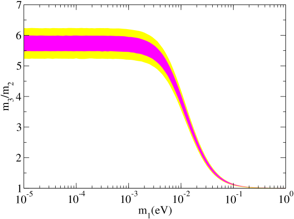
Figure 1: Experimental mass ratio of the two heavier neutrinos, $m_{2}/m_{3}$, vs. the mass of the lightest, $m_{1}$, in the case of normal hierarchy.

This contrasts to the hierarchy observed in quarks and charged leptons, where the typical mass ratios are ${\cal O}(20)$ (for $d-$quarks and $\mu$/$\tau$ leptons) and ${\cal O}(300)$ (for $u-$quarks and $e$/$\mu$ leptons) [3]. Of course, if the $\nu-$spectrum is quasi degenerate or with inverted hierarchy, the difference with the mass pattern of the other fermions is much more conspicuous. In any case we can safely conclude that the hierarchy between the two heaviest neutrinos is much softer than the one for the corresponding quarks or charged leptons.

According to the see-saw mechanism [4], which is the most popular mechanism for generating neutrino masses, these arise in a slightly more complicated way than the masses of quarks and charged leptons. Namely, beside the conventional Yukawa couplings between the Higgs, the left–handed and the right–handed neutrinos, one assumes Majorana masses for the right–handed ones. Upon decoupling of the latter, the light neutrino states have an effective Majorana mass matrix, ${\cal M}_{\nu}\propto{\bf Y}^{T}{\bf M}^{-1}{\bf Y}$, where ${\bf Y}$ is the initial matrix of Yukawa couplings and ${\bf M}$ is the Majorana mass matrix of the right-handed neutrinos. So, unlike quarks and charged leptons, neutrino masses are not proportional to the Yukawa couplings. Then one may wonder whether the peculiar pattern of neutrino masses can be a consequence of the peculiar way they are generated. If so, the spectrum of light neutrinos may shed light on the unknown features of the seesaw mechanism. In particular one may ask 1) How the present experimental data restrict the structure of the high-energy seesaw parameters and 2) Which choices, among the allowed ones, produce more naturally (i.e. without unpleasant fine-tunings) the observed pattern of neutrino masses. In other words, one can examine how possible and how plausible is for the seesaw mechanism to reproduce the experimental data, and what is the corresponding information that we can learn about the underlying high-energy theory. Also, from such analysis, one can hopefully extract hints on the still unknown part of the low-energy $\nu-$spectrum. The investigation of these questions and their physical implications is the goal of this paper.

In sect. 2 we fix the notation and put forward a basis-independent top-down parametrization for the see-saw, which is specially useful to study the pattern of $\nu-$masses. We discuss how the $V_{R}$ mixing matrix associated to ${\bf Y}$ plays here a key role. In sect. 3 we analyze the 2-neutrino case, as a simple and useful warm-up. In sect. 4 we study the 3-neutrino case. We give general analytical results, completing (and confirming) them with numerical surveys. We pay special attention to the possibility that the $\nu-$spectrum could arise from hierarchical Yukawa couplings, as for the other fermions, and work out the required structure of the high energy parameters and some consequences for the unknown part of the low-energy $\nu-$spectrum. In sect. 5 we explore suggestive ansätze for the $V_{R}$, showing in particular that identifying $V_{R}$ and $V_{\rm CKM}$, as well as $\nu-$ and $u-$quark Yukawa couplings can reproduce the experimental $\nu-$spectrum in a highly non-trivial way, which is remarkable. In sections 5 and we present the conclusions and an outlook discussing physical implications of these results. Finally, in the Appendix we give useful formulas concerning the eigenvalues of a (general or not) matrix.

2 Bottom-up and Top-down parametrizations of the see-saw

2.1 Notation and conventions

We will use a standard notation that can be used for both the Standard Model (SM) and the supersymmetric (SUSY) versions of the seesaw mechanism. The seesaw Lagrangian is given by

$${\cal L}\ \ \supset\ \ e_{R}^{c\ T}{\bf Y_{e}}L\cdot\bar{H}\ +\ \nu_{R}^{c\ T}{\bf Y}L\cdot H\ -\ {1\over 2}\nu_{R}^{c\ T}{\bf M}\nu_{R}^{c}\ +\ {\rm h.c.}$$ (2)

where $L_{i}$ ($i=e,\mu,\tau$) are the left-handed lepton doublets (generation indices are suppressed), $(e_{R}^{c})_{i}$ are the charged lepton singlets, ${\nu_{R}}_{i}$ the right-handed neutrino singlets and $H$ is the (hypercharge $=+1/2$) Higgs doublet. ${\bf Y_{e}},{\bf Y}$ are the $3\times 3$ matrices of charged-leptons and neutrino Yukawa couplings. Finally, ${\bf M}$ is a $3\times 3$ Majorana mass matrix for the right-handed neutrinos. Below ${\bf M}$ we can integrate out the right-handed neutrinos, obtaining the usual effective Lagrangian that contains a Majorana mass term for the left-handed neutrinos:

$$\delta{\cal L}=-{1\over 2}\nu^{T}{\cal M}_{\nu}\nu+h.c.$$ (3)

where

$${\cal M}_{\nu}=v^{2}\ \kappa\ ,$$ (4)

with $v=\langle H^{0}\rangle\simeq 174\ {\rm GeV}$ and

$${\bf\kappa}={\bf Y}^{T}{\bf M}^{-1}{\bf Y}$$ (5)

The previous equations are valid for a SUSY theory understanding all the fields in eqs.(2, 3) as superfields, and replacing ${\cal L}\rightarrow W$, $\delta{\cal L}\rightarrow\delta W$, i.e. the superpotential and the effective superpotential (with no h.c. terms). In addition $H\rightarrow H_{2}$, i.e. the (hypercharge $=+1/2$) SUSY Higgs doublet and $\langle H^{0}\rangle\rightarrow\langle H^{0}_{2}\rangle=v\sin\beta$, with $\tan\beta\equiv\langle H^{0}_{2}\rangle/\langle H^{0}_{1}\rangle$, as usual.

Working in the basis in which the charged-lepton Yukawa matrix (${\bf Y_{e}}$) and gauge interactions are flavour-diagonal, the neutrino mass matrix, ${\cal\kappa}$, can be expressed as

$${\bf\kappa}=U_{\rm MNS}^{*}\ D_{\bf\kappa}\ U_{\rm MNS}^{\dagger},\;\;\;\;\;\;\;D_{\kappa}\equiv{\rm diag}(\kappa_{1},\kappa_{2},\kappa_{3}),$$ (6)

where $\kappa_{i}\geq 0$ (with the convention $\kappa_{1}\leq\kappa_{2}\leq\kappa_{3}$ and thus $m_{1}\leq m_{2}\leq m_{3}$) and $U_{\rm MNS}$ is a unitary matrix that can be written as

$$U_{\rm MNS}=V\cdot{\mathrm{d}iag}(e^{-i\phi/2},e^{-i\phi^{\prime}/2},1)\ \ ,$$ (7)

where $\phi$ and $\phi^{\prime}$ are CP violating phases (if different from $0$ or $\pi$) and $V$ has the ordinary form of a CKM matrix

$$V=\pmatrix{c_{13}c_{12}&c_{13}s_{12}&s_{13}e^{-i\delta}\cr-c_{23}s_{12}-s_{23}s_{13}c_{12}e^{i\delta}&c_{23}c_{12}-s_{23}s_{13}s_{12}e^{i\delta}&s_{23}c_{13}\cr s_{23}s_{12}-c_{23}s_{13}c_{12}e^{i\delta}&-s_{23}c_{12}-c_{23}s_{13}s_{12}e^{i\delta}&c_{23}c_{13}\cr}.$$ (8)

Finally, note that the observable neutrino masses are given by

$$m_{i} = v^{2}\kappa_{i}\;\;\;\;\;\;\;\;\;({\rm SM})$$

$$m_{i} = v^{2}\sin^{2}\beta\ \kappa_{i}\;\;\;\;\;\;({\rm SUSY})$$ (9)

Since we will be mainly interested in the $m_{i}/m_{j}=\kappa_{i}/\kappa_{j}$ ratios, we will work most of the time with $\kappa_{i}$ rather than with $m_{i}$. This avoids the proliferation of annoying $v^{2}$, $v^{2}\sin^{2}\beta$ factors and permits a unified treatment of the SM and SUSY cases [note that eq.(5) is the same for both cases]. Actually, all the results in the paper are equally valid for the SM and the SUSY cases, except for some slight differences due to radiative effects discussed in sect. 5.

2.2 Basis-independent quantities

In order to perform basis-independent analyses, it is extremely convenient to work with basis-independent quantities. For this matter, note that under a change of basis

$$\nu_{L}\rightarrow X_{L}\nu_{L}\;\;,\;\;\;\;\nu_{R}\rightarrow X_{R}\nu_{R}\$$ (10)

($X_{L,R}$ are arbitrary unitary matrices), the Yukawa and mass matrices transform as

$${\bf Y}\rightarrow X_{R}^{\dagger}{\bf Y}X_{L}\;\;,\;\;\;\;{\bf M}\rightarrow X_{R}^{\dagger}{\bf M}X_{R}^{*}\;\;,\;\;\;\;\kappa\rightarrow X_{L}^{T}\kappa X_{L}$$ (11)

Now the low-energy neutrino Lagrangian, eq.(3), contains 9 independent (i.e. not absorbable in field redefinitions) parameters. They correspond to the three mass “eigenvalues” $\kappa_{i}$ (strictly speaking they are the positive square roots of the $\kappa\kappa^{\dagger}$ eigenvalues) and the six parameters of $U_{\rm MNS}$, which is by construction a basis-independent quantity (it is defined in a particular and well-determined basis of the $\nu_{L}$ fields).

On the other hand the see-saw (high-energy) Lagrangian, eq.(2), contains 18 independent parameters. These can be defined in the following way. From eq.(11) is clear that one can always go to a $\nu_{R}$ basis where ${\bf M}$ is diagonal, with positive entries:

$${\bf M}\rightarrow{\rm diag}(M_{1},M_{2},M_{3})\equiv D_{M}$$ (12)

where we adopt the convention $M_{1}\leq M_{2}\leq M_{3}$. Obviously $M_{i}$ are basis-independent quantities. Working in the $\nu_{L}$ and $\nu_{R}$ bases where ${\bf Y_{e}}$ and ${\bf M}$, respectively, are diagonal, the neutrino Yukawa matrix, ${\bf Y}$, can be expressed as

$${\bf Y}=V_{R}D_{Y}V_{L}^{\dagger},\;\;\;\;\;D_{Y}\equiv{\rm diag}(y_{1},y_{2},y_{3}),$$ (13)

where, again, $y_{i}\geq 0$ and $y_{1}\leq y_{2}\leq y_{3}$. The three $y_{i}$ parameters are obviously basis-independent quantities. Besides $M_{i}$ and $y_{i}$, there are 12 independent high-energy parameters contained in $V_{L},V_{R}$. Generically, both matrices can be written ${\bf\Phi_{1}}V{\bf\Phi_{2}}$, where ${\bf\Phi_{1,2}}$ are diagonal unitary matrices and $V$ has the same functional form as (8) [replacing the $\theta_{ij}$ angles and the $\delta$ phase by new $\theta_{ij}^{L}$, $\delta^{L}$ and $\theta_{ij}^{R}$, $\delta^{R}$ respectively]. However, for $V_{R}$ the ${\bf\Phi_{2}}$ matrix can be absorbed into the definition of $V_{L}$ [see eq.(13)], so

$$V_{R}=\pmatrix{e^{i\alpha_{1}}&&\cr&&\cr&e^{i\alpha_{2}}&\cr&&\cr&&1\cr}\pmatrix{c_{13}^{R}c_{12}^{R}&c_{13}^{R}s_{12}^{R}&s_{13}^{R}e^{-i\delta^{R}}\cr&&\cr-c_{23}^{R}s_{12}^{R}-s_{23}^{R}s_{13}^{R}c_{12}^{R}e^{i\delta^{R}}&c_{23}^{R}c_{12}^{R}-s_{23}^{R}s_{13}^{R}s_{12}^{R}e^{i\delta^{R}}&s_{23}^{R}c_{13}^{R}\cr&&\cr s_{23}^{R}s_{12}^{R}-c_{23}^{R}s_{13}^{R}c_{12}^{R}e^{i\delta^{R}}&-s_{23}^{R}c_{12}^{R}-c_{23}^{R}s_{13}^{R}s_{12}^{R}e^{i\delta^{R}}&c_{23}^{R}c_{13}^{R}}.$$ (14)

Likewise, for $V_{L}$ the ${\bf\Phi_{1}}$ matrix can be absorbed into phase definitions of $L=(\nu_{L},e_{L})^{T}$ and $e_{R}$ (keeping ${\bf Y_{e}}$ diagonal). Then $V_{L}$ has a structure similar to $U_{\rm MNS}$ in (7), i.e. $V_{L}=V(\theta_{12}^{L},\theta_{23}^{L},\theta_{13}^{L},\delta^{L})\times{\rm diag}(e^{i\beta_{1}},e^{i\beta_{2}},1)$. Hence, $V_{L}$ and $V_{R}$ have 6 independent parameters each, which, beside $M_{i}$ and $y_{i}$, complete the 18 independent parameters of the see-saw Lagrangian.

In summary, in the see-saw framework, the 18 (9) independent parameters of the high(low)-energy neutrino Lagrangian are given by the following basis-independent quantities:

$$\begin{array}[]{ccc}{\rm High-Energy}&&{\rm Low-Energy}\\ &&\\ y_{i}&&\kappa_{i}\\ M_{i}&&U_{\rm MNS}\\ V_{R}&\longrightarrow&\\ V_{L}&&\\ $------------$&&$------------$\\ 18\ {\rm parameters}&&9\ {\rm parameters}\end{array}$$ (23)

2.3 Bottom-up and Top-down parametrizations

Since the number of independent parameters of the see-saw mechanism is larger in the high-energy than in the effective theory, one finds often the problem of using the available (low-energy) experimental information to constrain the high-energy parameters. This is a bottom-up problem. It was shown in ref. [6] that, working in the basis where ${\bf Y_{e},M}$ are diagonal and positive, for given $D_{\kappa}$, $U_{\rm MNS}$, the Yukawa matrix ${\bf Y}$ has the form

$${\bf Y}=D_{\sqrt{M}}RD_{\sqrt{\kappa}}U_{\rm MNS}^{\dagger}$$ (24)

where $D_{\sqrt{M}}=\sqrt{D_{M}}$ (with $M_{i}$ arbitrary) and $R$ is a complex orthogonal matrix (with three arbitrary complex angles). Thus $D_{M}$ and $R$ contain the 9 additional parameters of the high-energy theory with respect to the low-energy one. Eq.(24) represents a bottom-up parametrization of the see-saw. If desired, one can extract $y_{i}$, $V_{L}$ and $V_{R}$ from ${\bf Y}$ upon diagonalization.

However, for some kinds of problems it is more convenient a top-down parametrization, i.e. a way to obtain, as directly as possible, the physical low-energy parameters from the high-energy ones. This is precisely the sort of problem considered here: what kind of low-energy neutrino spectrum can we naturally expect, starting with reasonable or well-motivated choices of the high-energy parameters. Obviously, starting with the high-energy parameters in (23) one can use eqs.(13, 5) to write $\kappa$ in the basis where ${\bf Y_{e},M}$ are diagonal

$$\kappa={\bf Y^{T}}D_{M^{-1}}{\bf Y}=V_{L}^{*}D_{Y}V_{R}^{T}D_{M^{-1}}V_{R}D_{Y}V_{L}^{\dagger}\ ,$$ (25)

and then, upon diagonalization, determine $U_{MNS}$ and $\kappa_{i}$. Nevertheless it would be useful to find a more direct way to extract the neutrino masses, $\kappa_{i}$, from the high-energy parameters. To this end it is interesting to notice that $\kappa_{i}$ do not depend on $V_{L}$. In particular, they can be obtained upon diagonalization of

$$\kappa^{\prime}=D_{Y}V_{R}^{T}D_{M^{-1}}V_{R}D_{Y}\ ,$$ (26)

which is simply $\kappa$ after redefining $\nu_{L}$ as in eq.(10) with $X_{L}=V_{L}$. This means that $D_{\kappa}=W_{L}^{T}\kappa^{\prime}W_{L}$ for a certain unitary $W_{L}$ matrix, or, in other words,

$$D_{\kappa^{2}}={\rm Eigenv}\{\kappa^{\prime}\kappa^{\prime\dagger}\}$$ (27)

Therefore, given $D_{Y}$ and $D_{M}$, the $V_{R}$ matrix tells the values of $\kappa_{i}$. $V_{L}$ and $U_{\rm MNS}$ get completely decoupled from this flux of information: note that 1) eq.(27) does not depend on $V_{L}$ and 2) the connection of $V_{L}$ and $U_{\rm MNS}$ is given by

$$U_{\rm MNS}=V_{L}W_{L}$$ (28)

where $W_{L}$ has been defined after eq.(26). This means that for any choice of $V_{R}$, one can always choose $V_{L}$ so that the experimental $U_{\rm MNS}$ is reproduced.

Eqs.(27, 28) [with $\kappa^{\prime}$, $W_{L}$ defined in eq.(26) and the lines below] represent a top-down parametrization of the see-saw which is useful for our purposes. The $V_{R}$ matrix, in particular, plays here a similar role as the $R$ matrix in the bottom-up parametrization (24). They encode the flux of information about matrix eigenvalues along the top-down and bottom-up directions,

$$D_{Y},\ D_{M}\;\;\;\stackrel{{\scriptstyle V_{R}}}{{\longrightarrow}}\;\;\;D_{\kappa}$$ (29)

$$D_{\kappa},\ D_{M}\;\;\;\stackrel{{\scriptstyle R}}{{\longrightarrow}}\;\;\;D_{Y}\;,$$ (30)

through eqs.(24, 27) respectively. $U_{\rm MNS}$ gets completely decoupled from this flux of information and can always be fitted. [This has been just explained for the top-down parametrization. For the bottom-up one, note from (24) that $D_{Y}$ depends on $D_{\kappa}$, $D_{M}$ and $R$, but not on $U_{\rm MNS}$.] Hence, it is not surprising that $V_{R}$ and $R$ contain the same number of parameters (6 for three families of neutrinos). The connection between them is given by

$$YY^{\dagger}=D_{\sqrt{M}}RD_{\kappa}R^{\dagger}D_{\sqrt{M}}=V_{R}D_{Y^{2}}V_{R}^{\dagger}\ .$$ (31)

It is worth mentioning that $V_{R}$ has a precise physical meaning: it measures the misalignment between ${\bf Y}$ and ${\bf M}$. If $V_{R}$ is non-diagonal, there is no $\nu_{R}$ basis in which ${\bf Y}$ and ${\bf M}$ can get simultaneously diagonal. The $V_{R}$ entries can be identified as genuine physical inputs (and in fact they play a relevant role in certain physical processes, as those related to leptogenesis). On the other hand, $R$ has a more obscure physical meaning, even though it is a useful tool for phenomenological analyses.

3 The 2-neutrino system

Although the case of two families of (left and right) neutrinos is obviously non-realistic, it is very useful in order to gain intuition about the form of the low-energy spectrum for typical high-energy inputs. In this case $V_{R}$ has the form

$$V_{R}=\left[\begin{array}[]{cc}e^{i\alpha}&\\ &1\end{array}\right]\ \left[\begin{array}[]{cc}c^{R}&s^{R}\\ -s^{R}&c^{R}\end{array}\right]\$$ (36)

We will first obtain some simple and general relations involving $V_{R}$, $D_{M}$, $D_{Y}$ and $D_{\kappa}$, which however contain much information. In particular they put useful constraints on $V_{R}$ to achieve a soft normal hierarchy, $\kappa_{2}/\kappa_{1}\sim 6$, or quasi-degeneracy, $\kappa_{2}/\kappa_{1}\sim 1$ (which for two neutrinos is equivalent to a inverse hierarchy). The techniques used for this general analysis will be useful for the 3-neutrino case, to be studied in the next section.

Then we will get exact results by solving analytically the secular equation (27) [something too cumbersome for three families].

3.1 General results

From eqs.(26, 27) is clear that

$${\rm det}\{D_{\kappa}\}=\kappa_{1}\kappa_{2}={y_{1}^{2}y_{2}^{2}\over M_{1}M_{2}}\ ,$$ (37)

which does not depend on $V_{R}$. On the other hand, the hierarchy between the physical masses, say $h$, can be written as

$$h\equiv{\kappa_{2}\over\kappa_{1}}={\kappa_{2}^{2}\over{\rm det}\{D_{\kappa}\}}\ ,$$ (38)

so any information about $\kappa_{2}$ translates automatically into $h$. Now, using eq.(27) we can obtain additional information on $\kappa_{2}$ from the fact that $\kappa^{\prime}\kappa^{\prime\dagger}$ is a positive hermitian matrix, which means in particular that its largest eigenvalue is larger than any diagonal entry, i.e.

$$\kappa_{2}^{2}\geq\left(\kappa^{\prime}\kappa^{\prime\dagger}\right)_{ii}=\sum_{j=1,2}|\kappa^{\prime}_{ij}|^{2}=y_{i}^{2}\sum_{j=1,2}y_{j}^{2}\left|(V_{R})_{ki}M_{k}^{-1}(V_{R})_{kj}\right|^{2}\ ,\;\;\;\;\;\;\;\;i=1,2$$ (39)

At this point we can try an ansatz for some of the high-energy parameters. Let us assume for the moment that the hierarchy between $y_{1}$ and $y_{2}$ is similar to the hierarchy of Yukawa couplings observed in charged fermions: $y_{2}/y_{1}={\cal O}(20-300)$. This means that the r.h.s. of eq.(39) is generically dominated by $\left(\kappa^{\prime}\kappa^{\prime\dagger}\right)_{22}$, in particular by the term proportional to $y_{2}^{4}$:

$$\kappa_{2}^{2}\geq\left(\kappa^{\prime}\kappa^{\prime\dagger}\right)_{22}={y_{2}^{4}\over M_{1}^{2}}\left|(V_{R})_{12}^{2}+{M_{1}\over M_{2}}(V_{R})_{22}^{2}\right|^{2}+{\cal O}\left({y_{1}^{2}y_{2}^{2}\over M_{1}^{2}}\right)$$ (40)

where the subdominant terms are positive. In fact, the previous inequality is typically close to an equality: note that from $\kappa_{2}^{2}\leq{\rm tr}(\kappa^{\prime}\kappa^{\prime\dagger})$, it follows that

$$\kappa_{2}^{2}-\left(\kappa^{\prime}\kappa^{\prime\dagger}\right)_{22}\leq\left(\kappa^{\prime}\kappa^{\prime\dagger}\right)_{11}={\cal O}\left({y_{1}^{2}y_{2}^{2}\over M_{1}^{2}}\right)\ .$$ (41)

Therefore, eq.(40) is an equality up to terms suppressed by ${\cal O}({y_{1}^{2}\over y_{2}^{2}})$.

Plugging eq.(40) into eq.(38), we obtain an exact inequality for $h$,

$$h={\kappa_{2}\over\kappa_{1}}\geq{y_{2}^{2}\over y_{1}^{2}}{M_{2}\over M_{1}}\left|(V_{R})_{12}^{2}+{M_{1}\over M_{2}}(V_{R})_{22}^{2}\right|^{2}$$ (42)

Clearly, for random values of the $V_{R}$ entries we expect a low-energy hierarchy $h={\cal O}\left({y_{2}^{2}\over y_{1}^{2}}{M_{2}\over M_{1}}\right)$, much stronger than that of Yukawa couplings and, of course, than the experimental one, $h^{exp}\lower 3.01385pt\hbox{$\;\stackrel{{\scriptstyle\textstyle<}}{{\sim}}\;$}6$. E.g. for $M_{1}\simeq M_{2}$ we expect $h={\cal O}(10^{2-5})$; for $M_{2}/M_{1}\sim y_{2}/y_{1}$ we expect $h={\cal O}(10^{3-7})$.

Consequently, either we give up the natural assumption that the Yukawa couplings for neutrinos present a hierarchy similar to the other fermions’, or we accept that the $(V_{R})$ entries are far from random. (This is already a strong conclusion that holds for the three-generation case, as we will see in the next section.) Let us take the second point of view and determine the constraints on $V_{R}$ to achieve degeneracy or soft hierarchy in the neutrino spectrum, $h\simeq 1$, $h\lower 3.01385pt\hbox{$\;\stackrel{{\scriptstyle\textstyle<}}{{\sim}}\;$}6$ respectively.

Let us first consider the degenerate ($h=1$) case, i.e. $\kappa_{1}^{2},\kappa_{2}^{2}\rightarrow y_{1}^{2}y_{2}^{2}/(M_{1}M_{2})$. Then, if $V_{R}$ has real entries, eq.(42) requires $(V_{R})_{12}^{4}\leq{y_{1}^{2}\over y_{2}^{2}}{M_{1}\over M_{2}}\ll 1$ [ie. $s^{R}\simeq 0$ in the parametrization (36)]. In addition, taking $i=1$ in (39), we get an extra inequality for $\kappa_{2}$

$$\kappa_{2}^{2}\geq{y_{1}^{4}\over M_{1}^{2}}\left|(V_{R})_{11}^{2}+{M_{1}\over M_{2}}(V_{R})_{21}^{2}\right|^{2}.$$ (43)

Multiplying (42) and (43) it is straightforward to check that the degenerate case is only obtainable when $(V_{R})_{21}=0$ (i.e. $s^{R}=0$) and, besides, $M_{2}/M_{1}=y_{2}^{2}/y_{1}^{2}$.

On the other hand, if $V_{R}$ has complex entries [$\alpha\neq 0,\pi$ in eq.(36)], a cancellation inside the r.h.s. of (40) is possible (in the absence of such cancellation the previous results essentially hold). This requires

$$(V_{R})_{12}^{2}\simeq-{M_{1}\over M_{2}}(V_{R})_{22}^{2}\;\;,$$ (44)

which in turn implies $\alpha\simeq\pm\pi/2$ in (36) (in the next subsection we will show that $\alpha=\pm\pi/2$ exactly). In addition, $M_{1}/M_{2}$ cannot be arbitrarily small. From (44) we see that very small $M_{1}/M_{2}$ implies $|(V_{R})_{21}|\ll 1$, $|(V_{R})_{22}|=|(V_{R})_{11}|\simeq 1$, which plugged into (43) gives $M_{1}/M_{2}\lower 3.01385pt\hbox{$\;\stackrel{{\scriptstyle\textstyle>}}{{\sim}}\;$}y_{1}^{2}/y_{2}^{2}$, thus setting a lower bound on $M_{1}/M_{2}$. Eq.(44) tells that, unless $M_{2}/M_{1}={\cal O}(1)$, the degeneracy can only be obtained by fine-tuning $s^{R}$ to a very small, but different from zero, value. (This is the case in particular for $M_{2}/M_{1}\simeq y_{2}/y_{1}$.) For random values of $s^{R}$ one is led to a huge hierarchy between the physical masses, as expected.

Let us now say how the previous conditions are relaxed if, instead of exact degeneracy ($h=1$), we require a soft hierarchy ($h\lower 3.01385pt\hbox{$\;\stackrel{{\scriptstyle\textstyle<}}{{\sim}}\;$}6$). For the real case we get a relaxed condition on the $M_{i}$ hierarchy: $h^{-1}\lower 3.01385pt\hbox{$\;\stackrel{{\scriptstyle\textstyle<}}{{\sim}}\;$}(M_{1}/M_{2})(y_{2}^{2}/y_{1}^{2})\lower 3.01385pt\hbox{$\;\stackrel{{\scriptstyle\textstyle<}}{{\sim}}\;$}h$. The upper bound corresponds to $s^{R}=0$. Otherwise a tuning of $s^{R}$ is required. For the complex case, whenever a cancellation inside eq.(40) is needed, the same condition (44) is obtained, thus requiring a small and tuned value of $s^{R}$. This occurs in particular for $M_{2}/M_{1}\simeq y_{2}/y_{1}$.

In summary, starting with a hierarchy of neutrino Yukawa couplings similar to that for the charged fermions leads typically to a very strong hierarchy of low-energy neutrino masses (unlike the observed one). Nevertheless, adjusting the $V_{R}$ entries it is possible to get the desired degeneracy or soft hierarchy at low-energy. The price is a fine-tuning between $y_{2}/y_{1}$, $M_{2}/M_{1}$ and $V_{R}$. Normally a very small, but different from zero angle in eq.(36) is required. If nature had just two species of neutrinos we would conclude that, unless a theoretical reason is found for this tuning, the see-saw mechanism cannot naturally lead to the observed low-energy neutrino spectrum if one starts with hierarchical neutrino Yukawa couplings similar to those of other fermions. (This applies to the model with two right-handed neutrinos and three left-handed neutrinos mentioned in footnote 3.)

3.2 Some exact results

For the 2-neutrino system, the mass eigenvalues can be obtained from eq.(27) in terms of the high-energy parameters in a completely analytical way. The results are particularly simple and illustrative for the degenerate case. Then eq.(27) can be written as $\kappa_{\rm d}^{2}{\bf 1}=\kappa^{\prime}\kappa^{\prime\dagger}$, with $\kappa_{\rm d}^{2}\equiv\kappa_{1}^{2}=\kappa_{2}^{2}=y_{1}^{2}y_{2}^{2}/(M_{1}M_{2})$. Consequently,

$$D_{M^{-1}}V_{R}D_{Y^{2}}V_{R}^{\dagger}D_{M^{-1}}=\kappa_{\rm d}^{2}V_{R}^{*}D_{Y^{-2}}V_{R}^{T}$$ (45)

Comparing the matrix entries of the two sides one concludes that the degeneracy is only achieved when

$$\alpha=\pi/2\ ,\;\;\;\;\;\cos^{2}\theta^{R}=\frac{M_{2}y^{2}_{2}-M_{1}y^{2}_{1}}{(M_{1}+M_{2})(y^{2}_{2}-y^{2}_{1})}\ ,$$ (46)

which implies in turn

$$\frac{y^{2}_{1}}{y^{2}_{2}}\leq\frac{M_{1}}{M_{2}}\ \ .$$ (47)

This confirms the fact that for any choice of $y_{i}$, $M_{i}$ satisfying the inequality (47), there is a choice of $V_{R}$ [given by eq.(46)] that produces exactly degenerate neutrinos, $\kappa_{1}=\kappa_{2}$.

On the other hand, one can check that the degeneracy is generically achieved thanks to a fine-tuning of the high-energy parameters. This is illustrated for $y_{2}/y_{1}=M_{2}/M_{1}=300$ (i.e. the same hierarchy as $u-$quarks) in Fig. 2, which shows the mass-ratio $m_{2}/m_{1}=\kappa_{2}/\kappa_{1}$ a function of $\theta^{R}$ for different values of the $\alpha$ phase. As expected, the exact degeneracy is only possible for $\alpha=\pi/2$ and at a very small (but different from zero) value of $\theta^{R}$ [see eq.(46) and the discussion after eq.(44)]. Changing $\theta^{R}$ and $\alpha$ from their critical values, even if very slightly, pushes rapidly $m_{2}/m_{1}$ out from the allowed experimental region (yellow band in the figure). For larger values of $\theta^{R}$, one gets $m_{2}/m_{1}\rightarrow{\cal O}\left({y_{2}^{2}\over y_{1}^{2}}{M_{2}\over M_{1}}\right)$, in agreement with the discussion of subsect. 3.1. To this respect, notice that in the figure only a small range of $\theta^{R}$ values has been represented (for the sake of clarity).

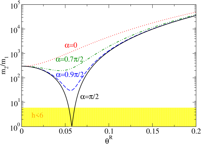
Figure 2: Mass-ratio $m_{2}/m_{1}$ in a 2-neutrino system vs. the $\theta^{R}$ angle for several values of the $\alpha-$phase (see the notation of eq. (36)) when $y_{1}:y_{2}=M_{1}:M_{2}=1:300$.

The conclusions are similar when $M_{1}\simeq M_{2}$, the only difference being that the critical value of $\theta^{R}$ is not small.

4 The 3-neutrino system

Let us now examine the realistic case with three neutrino species and a hierarchy between the two heavy ones, $h=m_{3}/m_{2}=\kappa_{3}/\kappa_{2}$, in the experimental range: from $h\simeq 1$ (quasi-degeneracy or inverse hierarchy) to $h\simeq 6$ (normal but soft hierarchy).

From the results of the previous section, we can already foresee some conclusions. First, to achieve a neutrino spectrum where the three neutrinos are quasi-degenerate or present a soft hierarchy will be probably as unnatural as for the 2-neutrino case. We will see that this indeed the case. On the other hand, to achieve the actual experimental constraint, namely soft hierarchy or quasi-degeneracy just for the two heavy neutrinos (the latter case corresponds to an inverse hierarchy) can be much easier. Eg. if $V_{R}$ has only sizeable entries in $\{1,2\}$ box, (i.e. $\theta_{23}=\theta_{13}=0$) $\kappa_{1}$ ($\kappa_{2}$) will decrease (increase) significantly, as $\theta_{12}$ departs from zero, while $\kappa_{3}$ will not change. In consequence we expect in this case a very large $\kappa_{2}/\kappa_{1}$ hierarchy but a softened $\kappa_{3}/\kappa_{2}$ one. This is consistent with experiment and does not imply fine-tunings (only small, but not tuned, values for certain angles). As we will see, other possibilities can also work, but they are not very different from the one just out-lined.

4.1 General results

Let us recall that the neutrino masses, $\kappa_{i}$, depend on the high-energy parameters, $y_{i},M_{i},V_{R}$ through eq.(27). As for the 2-neutrino case, the determinant

$${\rm det}\{D_{\kappa}\}=\kappa_{1}\kappa_{2}\kappa_{3}={y_{1}^{2}y_{2}^{2}y_{3}^{2}\over M_{1}M_{2}M_{3}}\ ,$$ (48)

does not depend on $V_{R}$. The hierarchy between the two heavy neutrino masses can be written as

$$h={m_{3}\over m_{2}}={\kappa_{3}\over\kappa_{2}}={\kappa_{3}^{2}\kappa_{1}\over{\rm det}\{D_{\kappa}\}}\ ,$$ (49)

Now, in order to get information about $h$ we need information on $\kappa_{3},\kappa_{1}$.

Using the fact [eq.(27)] that $\kappa_{i}^{2}$ are the eigenvalues of $\kappa^{\prime}\kappa^{\prime\dagger}$, which is a positive hermitian matrix, we can write

$$\kappa_{3}^{2}\geq\left(\kappa^{\prime}\kappa^{\prime\dagger}\right)_{ii}=\sum_{j=1,2,3}|\kappa^{\prime}_{ij}|^{2}=y_{i}^{2}\sum_{j=1,2,3}y_{j}^{2}|(V_{R})_{ki}M_{k}^{-1}(V_{R})_{kj}|^{2}\ ,\;\;\;\;\;\;\;\;i=1,2,3$$ (50)

At this point we can try again an ansatz for the spectrum of high-energy parameters. So let us assume for the moment that the hierarchy between the $y_{i}$ is similar to the hierarchy of Yukawa couplings observed in charged fermions: $y_{3}/y_{2},\ y_{2}/y_{1}={\cal O}(20-300)$. Then eq.(50) is generically dominated by $\left(\kappa^{\prime}\kappa^{\prime\dagger}\right)_{33}$, in particular by the term proportional to $y_{3}^{4}$, which corresponds to $i=j=3$:

$$\kappa_{3}^{2}\geq\left(\kappa^{\prime}\kappa^{\prime\dagger}\right)_{33}={y_{3}^{4}\over M_{1}^{2}}\left|(V_{R})_{13}^{2}+{M_{1}\over M_{2}}(V_{R})_{23}^{2}+{M_{1}\over M_{3}}(V_{R})_{33}^{2}\right|^{2}+{\cal O}\left({y_{3}^{2}y_{2}^{2}\over M_{1}^{2}}\right)$$ (51)

where the subdominant terms are positive. As for two neutrinos, the previous inequality is typically close to an equality: from $\kappa_{3}^{2}\leq{\rm tr}(\kappa^{\prime}\kappa^{\prime\dagger})$, it follows that

$$\kappa_{3}^{2}-\left(\kappa^{\prime}\kappa^{\prime\dagger}\right)_{33}\leq\left(\kappa^{\prime}\kappa^{\prime\dagger}\right)_{11}+\left(\kappa^{\prime}\kappa^{\prime\dagger}\right)_{22}={\cal O}\left({y_{3}^{2}y_{2}^{2}\over M_{1}^{2}}\right)\ ,$$ (52)

so (51) holds as an equality up to ${y_{2}^{2}\over y_{3}^{2}}$–suppressed terms.

On the other hand we can obtain information on $\kappa_{1}$ by considering $\kappa^{\prime-1}(\kappa^{\prime-1})^{\dagger}$, which is a positive hermitian matrix with $\kappa_{i}^{-2}$ eigenvalues. The largest eigenvalue, $\kappa_{1}^{-2}$, satisfies

$$\kappa_{1}^{-2}\geq\left(\kappa^{\prime-1}(\kappa^{\prime-1})^{\dagger}\right)_{ii}=\sum_{j=1,2,3}|\kappa^{\prime-1}_{ij}|^{2}=y_{i}^{-2}\sum_{j=1,2,3}y_{j}^{-2}|(V_{R})_{ki}M_{k}(V_{R})_{kj}|^{2},\;\;\;i=1,2,3$$ (53)

This equation is typically dominated by $\left(\kappa^{\prime-1}(\kappa^{\prime-1})^{\dagger}\right)_{11}$, in particular by the $i=1,j=1$ term,

$$\kappa_{1}^{2}\leq{y_{1}^{4}\over M_{3}^{2}}\left|(V_{R})_{31}^{2}+{M_{2}\over M_{3}}(V_{R})_{21}^{2}+{M_{1}\over M_{3}}(V_{R})_{11}^{2}\right|^{-2}-{\cal O}\left({y_{1}^{6}\over y_{2}^{2}M_{3}^{2}}\right)$$ (54)

where the subdominant terms are negative (so ignoring them still represents an exact inequality). Again, this inequality is typically close to an equality: from $\kappa_{1}^{-2}\leq{\rm tr}\left[\kappa^{\prime-1}(\kappa^{\prime-1})^{\dagger}\right]$ it follows that

$$\kappa_{1}^{2}\geq\left[\sum_{i,j=1,2,3}|\kappa^{\prime-1}_{ij}|^{2}\right]^{-1}\ ,$$ (55)

which is dominated by $i=j=1$:

$$\kappa_{1}^{2}\geq{y_{1}^{4}\over M_{3}^{2}}\left|(V_{R})_{31}^{2}+{M_{2}\over M_{3}}(V_{R})_{21}^{2}+{M_{1}\over M_{3}}(V_{R})_{11}^{2}\right|^{-2}-{\cal O}\left({y_{1}^{6}\over y_{2}^{2}M_{3}^{2}}\right)$$ (56)

Note that in eq.(56) the subdominant terms are negative (so ignoring them here represents an approximate inequality). In any case, comparing (54) and (56), we see that eq.(54) holds as an equality up to ${y_{1}^{2}\over y_{2}^{2}}$–suppressed terms.

Similarly to the 2-neutrino case, plugging eqs.(51, 56) into eq.(49) we get an inequality for $h$,

$$h={m_{3}\over m_{2}}={\kappa_{3}\over\kappa_{2}}\ \lower 3.01385pt\hbox{$\;\stackrel{{\scriptstyle\textstyle>}}{{\sim}}\;$}\ {y_{3}^{2}\over y_{2}^{2}}{M_{2}\over M_{1}}{\left|(V_{R})_{13}^{2}+{M_{1}\over M_{2}}(V_{R})_{23}^{2}+{M_{1}\over M_{3}}(V_{R})_{33}^{2}\right|^{2}\over\left|(V_{R})_{31}^{2}+{M_{2}\over M_{3}}(V_{R})_{21}^{2}+{M_{1}\over M_{3}}(V_{R})_{11}^{2}\right|}\ .$$ (57)

From this expression it is clear that for random values of the $V_{R}$ entries we expect a low-energy hierarchy much stronger than that of Yukawa couplings.

Only for $y_{3}/y_{2}$, $M_{2}/M_{1}$ $={\cal O}(1)$ can the experimental value $h^{exp}\lower 3.01385pt\hbox{$\;\stackrel{{\scriptstyle\textstyle<}}{{\sim}}\;$}6$ be naturally obtained. For a $y_{i}/y_{j}$ hierarchy similar to quarks and charged leptons, we expect we expect $h={\cal O}(10^{2-5})$ if $M_{1}\simeq M_{2}\simeq M_{3}$, and $h={\cal O}(10^{3-7})$ if $M_{i}/M_{j}\sim y_{i}/y_{j}$ (which is probably a more attractive possibility), in any case way too large.

So we arrive to a similar conclusion as for two neutrinos: either we give up the natural assumption that the neutrino Yukawa couplings present a hierarchy similar to other fermions, or we accept that the $V_{R}$ entries are far from random. However, in this case “far from random” does not necessarily mean “fine-tuned”, as will be shown in subsect. 4.3.

We will devote subsects. 4.2 and 4.3 to determine the pattern of $V_{R}$ required to achieve the desired soft hierarchy (or quasi-degeneracy) for the three neutrinos or just for the two heavy ones respectively. Let us advance that since the absolute value in the denominator of (57) is $\leq 1$, then $\left|(V_{R})_{13}^{2}+{M_{1}\over M_{2}}(V_{R})_{23}^{2}+{M_{1}\over M_{3}}(V_{R})_{33}^{2}\right|^{2}\ll 1$ must be fulfilled in all cases.

Connection with models of anarchic neutrinos

We would like to make a very short digression about the use of the previous approach to analyze scenarios of anarchic neutrinos [9]. The basis-independent top-down formulation of the see-saw mechanism that we are using may be convenient to make statistical considerations about the high-energy parameters that define the theory, as is done in models of anarchic neutrinos. In particular, in the absence of additional assumptions, it makes sense to scan $y_{i}$ and the 6 parameters defining $V_{R}$ instead of the ${\bf Y}$ matrix, which contains 18 parameters (3 of them redundant and 6 not related to the neutrino masses).

Then, from (57) we notice that for average values of the $V_{R}$ entries, in particular for $|(V_{R})_{13}|^{2}\sim|(V_{R})_{31}|^{2}\sim 1/3$, we get a hierarchy $h\sim{1\over 3}{y_{3}^{2}\over y_{2}^{2}}{M_{2}\over M_{1}}$. Therefore the expectable pattern of neutrino masses depends crucially on the range in which the $y_{i},M_{i}$ parameters are allowed to vary. E.g. if one uses $y_{i}\in[1/a,a]y_{0}$, $M_{i}\in[1/a,a]M_{0}$, with $a>1$, one expects $h\sim a^{3}/3$.

4.2 Degeneracy or soft hierarchy for the three neutrinos

Let us first consider the case of completely degenerate low-energy neutrinos. From eq.(48) this means

$$\kappa_{1}^{2}=\kappa_{2}^{2}=\kappa_{3}^{2}\equiv\kappa_{\rm deg}^{2}=\left({y_{1}^{2}y_{2}^{2}y_{3}^{2}\over M_{1}M_{2}M_{3}}\right)^{2/3}$$ (58)

Now we will use the inequalities (50, 53) for $i=j=1,3$. This produces four inequalities, which are given by eqs.(51, 54) and

$$\kappa_{3}^{2}\geq{y_{1}^{4}\over M_{3}^{2}}\left|(V_{R})_{31}^{2}+{M_{3}\over M_{2}}(V_{R})_{21}^{2}+{M_{3}\over M_{1}}(V_{R})_{11}^{2}\right|^{2}$$ (59)

$$\kappa_{1}^{2}\leq{y_{3}^{4}\over M_{1}^{2}}\left|(V_{R})_{13}^{2}+{M_{2}\over M_{1}}(V_{R})_{23}^{2}+{M_{3}\over M_{1}}(V_{R})_{33}^{2}\right|^{-2}$$ (60)

Again we assume a strong hierarchy among the $y_{i}$, say similar to the hierarchy of Yukawa couplings observed in charged fermions: $y_{3}/y_{2},\ y_{2}/y_{1}={\cal O}(20-300)$. We do not assume a priori any particular hierarchy between the three $M_{i}$, except the conventional ordering $M_{1}\leq M_{2}\leq M_{3}$.

Let us suppose for the moment that there are no delicate cancellations among the terms in the right-hand sides of eqs.(51, 54, 59, 60). This means that the absolute value of each term inside the straight brackets is $\;\stackrel{{\scriptstyle\textstyle<}}{{\sim}}\;$ the absolute value of the sum of them (note that “$\;\stackrel{{\scriptstyle\textstyle<}}{{\sim}}\;$” becomes “$\leq$” for real $V_{R}$). Then, since ${y_{3}^{2}/M_{1}}\gg\kappa_{\rm deg}$, ${y_{1}^{2}/M_{3}}\ll\kappa_{\rm deg}$, it is clear from eqs.(51) and (54) that $|(V_{R})_{13}|^{2}\ll 1$ and $|(V_{R})_{31}|^{2}\ll 1$ respectively. Besides, the unitarity of $V_{R}$ implies that either a) $|(V_{R})_{23}|^{2},\ |(V_{R})_{32}|^{2}\ll 1$ or b) $|(V_{R})_{21}|^{2},\ |(V_{R})_{12}|^{2}\ll 1$, i.e. $V_{R}$ is approximately box-diagonal. Furthermore, looking at the $(V_{R})_{ij}^{2}$-term with smaller factor in eqs.(51) and (54) we obtain

$${y_{3}^{2}\over M_{3}}\lower 3.01385pt\hbox{$\;\stackrel{{\scriptstyle\textstyle<}}{{\sim}}\;$}\kappa_{\rm deg}\ ,\;\;\;\;\;\;\;\;{y_{1}^{2}\over M_{1}}\lower 3.01385pt\hbox{$\;\stackrel{{\scriptstyle\textstyle>}}{{\sim}}\;$}\kappa_{\rm deg}$$ (61)

respectively. This implies $M_{3}/M_{1}\ \lower 3.01385pt\hbox{$\;\stackrel{{\scriptstyle\textstyle>}}{{\sim}}\;$}y_{3}^{2}/y_{1}^{2}$. (This works similar to the case of two neutrinos, see eq.(47).) Suppose $V_{R}$ falls in the possibility a) above, which means $|(V_{R})_{33}|^{2}={\cal O}(1)$. Then eq.(60) implies $y_{3}^{2}/M_{3}\lower 3.01385pt\hbox{$\;\stackrel{{\scriptstyle\textstyle>}}{{\sim}}\;$}\kappa_{\rm deg}$ which, together with the first equation in (61), requires

$${y_{3}^{2}\over M_{3}}\simeq\kappa_{\rm deg}$$ (62)

This corresponds to the fact that $V_{R}$ is essentially diagonal, except in the 1-2 box. Eqs.(62, 58) imply ${y_{1}^{2}y_{2}^{2}\over M_{1}M_{2}}\simeq\kappa_{\rm deg}^{2}$. Due to the large $y-$hierarchy, this means ${y_{1}^{2}\over M_{2}}\ll\kappa_{\rm deg}\ll{y_{2}^{2}\over M_{1}}$. Applying this to the second term in the r.h.s. of eq.(54), we conclude $|(V_{R})_{21}|^{2}\ll 1$ (and $|(V_{R})_{11}|^{2}\simeq 1$, $|(V_{R})_{12}|^{2}\ll 1$ by unitarity). So $V_{R}$ is essentially ${\bf 1}$. Actually, from the third term of (59) we obtain ${y_{1}^{2}\over M_{1}}\lower 3.01385pt\hbox{$\;\stackrel{{\scriptstyle\textstyle<}}{{\sim}}\;$}\kappa_{\rm deg}$, which together with eq.(61), implies ${y_{2}^{2}\over M_{2}}\simeq\kappa_{\rm deg}$. Had we started with the possibility b) above, we would have obtained the same conclusion. In summary, if there are no precise cancellations in the r.h.s. of eqs.(51, 54, 59, 60), the only choice of high-energy parameters giving completely degenerate neutrinos is

$${y_{1}^{2}\over M_{1}}\simeq{y_{2}^{2}\over M_{2}}\simeq{y_{3}^{2}\over M_{3}}\simeq\kappa_{\rm deg}^{2}\ ,\;\;\;\;\;\;V_{R}\simeq{\bf 1}$$ (63)

This is similar to the 2-neutrino case.

If the $y_{i},M_{i},V_{R}$ parameters are not in the relation (63), we are forced to admit non-trivial cancellations between the various terms in the right-hand-sides of eqs.(51, 54, 59, 60). In particular, if such cancellation exists in the r.h.s. of eq.(51) and eq.(54), the constraints (61) [and the subsequent $M_{3}/M_{1}\ \lower 3.01385pt\hbox{$\;\stackrel{{\scriptstyle\textstyle>}}{{\sim}}\;$}y_{3}^{2}/y_{1}^{2}$ inequality] do not apply. Actually, for a wide range of $y_{i},M_{i}$ parameters, the entries of $V_{R}$ can be arranged so that the two cancellations take place and $\kappa_{1}=\kappa_{2}=\kappa_{3}=\kappa_{\rm deg}$ (see below for more details). However, this amounts to a very accurate (and thus unplausible) fine-tuning. This result cannot be easily appreciated if one just uses the bottom-up see-saw parametrization, eq.(24), since this automatically gives sets of working $y_{i}$ parameters for arbitrary $M_{i},R$. An intermediate situation occurs when the cancellation takes place “just” in one of the right-hand-sides of eqs.(51, 54, 59, 60). Eg. suppose that the cancellation just occurs in the r.h.s. of eq.(54). Then, from eqs.(51, 60) we easily conclude that ${y_{3}^{2}\over M_{2}}|(V_{R})_{23}|^{2}\lower 3.01385pt\hbox{$\;\stackrel{{\scriptstyle\textstyle<}}{{\sim}}\;$}\kappa_{\rm deg}\lower 3.01385pt\hbox{$\;\stackrel{{\scriptstyle\textstyle<}}{{\sim}}\;$}{y_{3}^{2}\over M_{3}}(1-|(V_{R})_{23}|^{2})^{-1}$, which implies that either ${y_{3}^{2}\over M_{3}}$ or ${y_{3}^{2}\over M_{2}}$ must be close to $\kappa_{\rm deg}$.

In any case, we have seen that unless the high-energy parameters satisfy (63), fine cancellations are required in order to obtain degenerate neutrinos. Then, in the absence of an explanation for such cancellations, we conclude that degenerate neutrinos are not natural within the see-saw framework if the neutrino Yukawa couplings present a hierarchy similar to other fermions. Let us also note that sometimes is stated that (see-saw) degenerate neutrinos naturally require degenerate right-handed Majorana masses, $M_{i}$, as well. Now we see that this is only true if the Yukawa couplings are degenerate as well, according to eq.(63). Otherwise a fine-tuning for the $V_{R}$ entries is needed, exactly as for other choices of $M_{i}$.

Let us now be more precise about what conditions must fulfill the $y_{i},M_{i}$ parameters in order to exist a choice of $V_{R}$ that implements degenerate neutrinos. First of all, notice that if ${y_{2}^{2}\over M_{2}}=\kappa_{\rm deg}$, the problem reduces to a 2-neutrino one, in this case the 1 and 3 neutrinos. [This occurs in particular when both the $y_{i}-$ and the $M_{i}-$hierarchies are regular, i.e. $y_{3}/y_{2}=y_{2}/y_{1}$, $M_{3}/M_{2}=M_{2}/M_{1}$.] Then, from the results of the previous section, we know that, provided $M_{3}/M_{1}\leq y_{3}^{2}/y_{1}^{2}$, there will be a non-trivial solution. The corresponding $V_{R}$ matrix is non-trivial in the 1–3 box. Since the $y_{3}^{2}/y_{1}^{2}$ ratio is normally very large, the fine-tuning in the values of the $V_{R}$ entries must be extremely precise. More generally, we can obtain necessary conditions for $y_{i},M_{i}$ in order to accommodate degenerate neutrinos as follows. Using the bottom-up see-saw parametrization (24), if neutrinos are degenerate we can write

$$YY^{\dagger}=\kappa_{\rm deg}\sqrt{D_{M}}RR^{\dagger}\sqrt{D_{M}}$$ (64)

where $\kappa_{\rm deg}$ is given by (58). Since $YY^{\dagger}$ is a positive hermitian matrix, its largest eigenvalue, $y_{3}^{2}$, must be larger than the diagonal entries, i.e.

$$y^{2}_{3}\geq\kappa_{\rm deg}\{M_{i}(RR^{\dagger})_{ii}\},\;\;\;\;i=1,2,3$$ (65)

Taking into account $(RR^{\dagger})_{ii}\geq 1$ (this can be readily checked using eg. the parametrization of $R$ given in ref. [6]) we finally obtain

$$y^{2}_{3}\geq\kappa_{\rm deg}M_{3}$$ (66)

A similar argument applied to the $(YY^{\dagger})^{-1}$ matrix leads to

$$y^{2}_{1}\leq\kappa_{\rm deg}M_{1}$$ (67)

Note that eqs.(66, 67) imply $M_{3}/M_{1}\leq y_{3}^{2}/y_{1}^{2}$. Let us stress that these are necessary but not sufficient conditions to guarantee the existence of a $V_{R}$ matrix producing degenerate neutrinos. Nevertheless the numerical analysis shows that in most cases satisfying the above conditions such $V_{R}$ matrix can be found. Note that conditions (66, 67) are only compatible with the constraints (61) [obtained under the assumption of no fine-tunings in $V_{R}$] when eq.(63) is fulfilled, in agreement with the previous discussion.

In summary, if neutrino Yukawa couplings present a hierarchy similar to other fermions, a spectrum of completely degenerate (or quasi-degenerate) neutrinos is possible but quite unnatural. For random $V_{R}$ the hierarchy of neutrino masses is actually much stronger than that of Yukawa couplings, in absolute conflict with experimental data. For $V_{R}={\bf 1}$ a degenerate spectrum if the Yukawa couplings, $y_{i}$, and the right-handed masses, $M_{i}$ are in the precise proportion (63). For arbitrary $y_{i}$, $M_{i}$ satisfying (66, 67) it is in general possible to find a particular $V_{R}$ giving degenerate neutrinos, but this amounts to a strong fine-tuning.

Finally, let us remark that these conclusions still hold (although somewhat softened) if instead degenerate neutrinos one demands hierarchical neutrinos with a soft hierarchy between the three families, e.g. $\kappa_{3}/\kappa_{2}\lower 3.01385pt\hbox{$\;\stackrel{{\scriptstyle\textstyle<}}{{\sim}}\;$}6$ (this is obliged by experimental data) and $\kappa_{2}/\kappa_{1}\lower 3.01385pt\hbox{$\;\stackrel{{\scriptstyle\textstyle<}}{{\sim}}\;$}6$ (this is just an hypothesis).

These results strongly suggest to consider soft hierarchy or quasi-degeneracy just for the two heavy neutrinos, which we study next.

4.3 Degeneracy or soft hierarchy for ${\bf m_{3}/m_{2}}$

We will focus now on the possibility of fulfilling $h={m_{3}\over m_{2}}={\kappa_{3}\over\kappa_{2}}\lower 3.01385pt\hbox{$\;\stackrel{{\scriptstyle\textstyle<}}{{\sim}}\;$}6$ (i.e. the only experimental constraint on the ratio of neutrino masses), starting with hierarchical Yukawa couplings. Again we will assume for the moment that the hierarchy between the $y_{i}$ is similar to the hierarchy of Yukawa couplings observed in charged fermions: $y_{3}/y_{2},\ y_{2}/y_{1}={\cal O}(20-300)$.

For convenience for the discussion we repeat here the previous bound (57) on the value of $h$,

$$h\lower 3.01385pt\hbox{$\;\stackrel{{\scriptstyle\textstyle>}}{{\sim}}\;$}{y_{3}^{2}\over y_{2}^{2}}{M_{2}\over M_{1}}{\left|(V_{R})_{13}^{2}+{M_{1}\over M_{2}}(V_{R})_{23}^{2}+{M_{1}\over M_{3}}(V_{R})_{33}^{2}\right|^{2}\over\left|(V_{R})_{31}^{2}+{M_{2}\over M_{3}}(V_{R})_{21}^{2}+{M_{1}\over M_{3}}(V_{R})_{11}^{2}\right|}\ ,$$ (68)

As discussed in subsect.4.1, this equation tells us that for random values of the $V_{R}$ entries we expect $h\sim{y_{3}^{2}\over y_{2}^{2}}{M_{2}\over M_{1}}\gg 6$. Therefore we need to imagine ways to get $h$ much smaller than the “random” result, preferably without fine-tunings. Obviously this is much easier to achieve if the combination of $V_{R}$ elements in the denominator of (68) is as large as possible. From (54) this corresponds to $\kappa_{1}$ as small as possible. Therefore generically it is far more natural to get the experimental result $h\lower 3.01385pt\hbox{$\;\stackrel{{\scriptstyle\textstyle<}}{{\sim}}\;$}6$ if the lightest neutrino presents a much stronger hierarchy than the two heavy ones, which is an interesting conclusion.

However, a denominator as large as possible is not enough to render $h\lower 3.01385pt\hbox{$\;\stackrel{{\scriptstyle\textstyle<}}{{\sim}}\;$}6$: the expression in straight brackets in the denominator is $\leq 1$, so a small numerator, $\left|(V_{R})_{13}^{2}+{M_{1}\over M_{2}}(V_{R})_{23}^{2}+{M_{1}\over M_{3}}(V_{R})_{33}^{2}\right|^{2}\ll 1$, is always obliged. If $M_{1}=M_{2}=M_{3}$ (i.e. degenerate right-handed neutrinos) this can only be accomplished by a cancellation between the various terms in the numerator. On the contrary, if $M_{1}\ll M_{2}\ll M_{3}$ this could be achieved without cancellations. We examine next the two cases separately.

${\bf M_{1}\ll M_{2}\ll M_{3}}$

If we do not allow fine cancellations in the numerator of eq.(68), this gets minimal when is dominated by the $(V_{R})_{33}^{2}$ term. This requires $|(V_{R})_{13}|^{2}$ and $|(V_{R})_{23}|^{2}$ $\ll 1$; more precisely $|(V_{R})_{13}|^{2}<M_{1}/M_{3}$ and $|(V_{R})_{23}|^{2}<M_{2}/M_{3}$. Then $(V_{R})_{31}^{2}$ in the denominator is also very small (by unitarity of $V_{R}$) and eq.(68) can normally be approximated as

$$h\lower 3.01385pt\hbox{$\;\stackrel{{\scriptstyle\textstyle>}}{{\sim}}\;$}{y_{3}^{2}\over y_{2}^{2}}{M_{1}\over M_{3}}{1\over|(V_{R})_{21}^{2}+{M_{1}\over M_{2}}(V_{R})_{11}^{2}|}\ .$$ (69)

In particular,

$$h\lower 3.01385pt\hbox{$\;\stackrel{{\scriptstyle\textstyle>}}{{\sim}}\;$}{y_{3}^{2}\over y_{2}^{2}}{M_{1}\over M_{3}}{1\over|(V_{R})_{21}|^{2}}\;\;\;\;\;\;\;\;\;{\rm if\;\;\;}|(V_{R})_{21}|^{2}\lower 3.01385pt\hbox{$\;\stackrel{{\scriptstyle\textstyle>}}{{\sim}}\;$}(M_{1}/M_{2}).$$ (70)

$$h\lower 3.01385pt\hbox{$\;\stackrel{{\scriptstyle\textstyle>}}{{\sim}}\;$}{y_{3}^{2}\over y_{2}^{2}}{M_{2}\over M_{3}}\;\;\;\;\;\;\;\;\;\;\;\;\;\;\;\;\;\;\;\;\;\;\;{\rm otherwise}\ \ .$$ (71)

E.g. if ${M_{i}/M_{j}}={y_{i}/y_{j}}$ (which we find a reasonable assumption) in a regular hierarchy, i.e. ${y_{1}\over y_{2}}={y_{2}\over y_{3}}$, then the case (70) becomes $h\lower 3.01385pt\hbox{$\;\stackrel{{\scriptstyle\textstyle<}}{{\sim}}\;$}|(V_{R})_{21}|^{-2}$. As a matter of fact, taking $|(V_{R})_{21}|=1$ and $(V_{R})_{11}$, $(V_{R})_{13}=0$, leads exactly to $\kappa_{3}=\kappa_{2}$ and thus inverse hierarchy. This can be easily checked using the exact results of subsect.3.2, since in this limit the problem involves only two neutrinos. More generally, for sizeable $|(V_{R})_{21}|^{2}$ we get a soft hierarchy for the two heavy neutrinos. E.g. for $|(V_{R})_{21}|^{2}\lower 3.01385pt\hbox{$\;\stackrel{{\scriptstyle\textstyle>}}{{\sim}}\;$}1/6$ we get $h\lower 3.01385pt\hbox{$\;\stackrel{{\scriptstyle\textstyle<}}{{\sim}}\;$}6$, in agreement with experiment. Notice that there are no delicate cancellations (and thus no fine-tuning) involved in this instance: changes in the $V_{R}$ entries amount to changes in $h$ in a similar proportion. On the other hand, for very small $|(V_{R})_{21}|$ (and thus very small $|(V_{R})_{12}|$ by unitarity) eq.(69) becomes $h\lower 3.01385pt\hbox{$\;\stackrel{{\scriptstyle\textstyle>}}{{\sim}}\;$}{y_{3}^{2}\over y_{2}^{2}}{M_{2}\over M_{3}}={y_{3}\over y_{2}}$, which is too large.

Let us stress that the above possibility of getting an experimentally viable $h$ with no fine-tunings requires very small $|(V_{R})_{13}|$, $|(V_{R})_{23}|$, and sizeable $|(V_{R})_{21}|$. This coincides exactly with the structure of the CKM matrix, which we find very suggestive. Actually, the coincidence is even stronger since the previous discussion suggests $|(V_{R})_{13}|^{2}\ll|(V_{R})_{23}|\ll|(V_{R})_{21}|=$ sizeable, as for CKM. We will turn to a more careful exam of this CKM-like form for $V_{R}$ in sect.5.

Another (less attractive) possibility to get a small numerator in eq.(68) is to allow for cancellations between the various terms inside the straight brackets. This requires $|(V_{R})_{13}|^{2}\lower 3.01385pt\hbox{$\;\stackrel{{\scriptstyle\textstyle>}}{{\sim}}\;$}M_{1}/M_{3}$ and/or $|(V_{R})_{23}|^{2}\lower 3.01385pt\hbox{$\;\stackrel{{\scriptstyle\textstyle>}}{{\sim}}\;$}M_{2}/M_{3}$. Still, this possibility requires very small $|(V_{R})_{13}|$. The largest possible value for $|(V_{R})_{13}|$ occurs when it cancels against the $(V_{R})_{23}^{2}$ term, so

$$|(V_{R})_{13}|^{2}\lower 3.01385pt\hbox{$\;\stackrel{{\scriptstyle\textstyle<}}{{\sim}}\;$}{M_{2}\over M_{3}}\ .$$ (72)

These results are illustrated in Fig. 3, where we show the density of allowed points in the $|(V_{R})_{13}|-|(V_{R})_{23}|$ plane for fixed values of $|(V_{R})_{12}|$ [this determines the $V_{R}$ matrix up to phases, according to eq.(14)] and $y_{1}:y_{2}:y_{3}$ $=1:300:9\times 10^{4}$, $M_{1}:M_{2}:M_{3}$ $=1:300:9\times 10^{4}$. In each point, we have evaluated $h$ for 1000 random values of the phases in $V_{R}$, and counted the number of points that are compatible with the observed hierarchy, $h\lower 3.01385pt\hbox{$\;\stackrel{{\scriptstyle\textstyle<}}{{\sim}}\;$}6$. White areas are excluded, while colored areas are allowed, corresponding the redder (darker in black and white printer) areas to the regions with higher density of allowed points. The reddest areas precisely correspond to the choices of $V_{R}$ that reproduce naturally (with no cancellations) the observed mass hierarchy. As discussed just before eq.(69), this occurs for $|(V_{R})_{13}|^{2}<M_{1}/M_{3}$ and $|(V_{R})_{23}|^{2}<M_{2}/M_{3}$, thus the size and shape of the reddest “rectangle”. The light blue (light grey in black and white) areas correspond to the choices of $V_{R}$ that can reproduce the observations with a certain amount of tuning. As argued above, for small $|(V_{R})_{12}|$ it is not possible to reproduce $h^{exp}$, unless a fine-tuning in the numerator of (68) takes place, thus the tiny light allowed areas for $|(V_{R})_{12}|^{2}\lower 3.01385pt\hbox{$\;\stackrel{{\scriptstyle\textstyle<}}{{\sim}}\;$}1/6$, in agreement with the previous discussion. The bound (72) is also clearly visible.

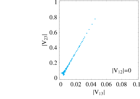
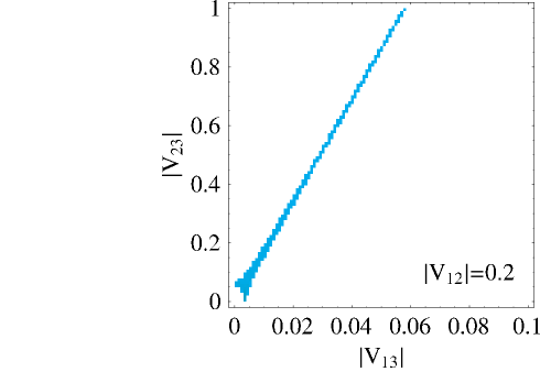
Figure 3: Region in the $|(V_{R})_{13}|-|(V_{R})_{23}|$ plane which gives $m_{3}/m_{2}\leq 6$ for some choice of the phases of $V_{R}$ (see eq.(14)). For each point, 1000 random choices are probed. The color indicates the fraction of unsuccessful choices: from red (complete success) to light blue. The scenario is defined by $M_{1}=M_{2}=M_{3}=y_{1}:y_{2}:y_{3}=1:300:9\times 10^{4}$. Each plot corresponds to a different value of $|(V_{R})_{12}|$. The dashed line in the last plot corresponds to the limit of unitarity of $V_{R}$, while the solid line corresponds to the approximate analytical bound discussed at eq. (73).

The shape of the complete allowed region can be analytically understood as follows. For not too small $|(V_{R})_{23}|^{2}$ [in particular when we allow for cancellations in the numerator of (68)], the denominator of (68) is dominated by $|(V_{R})_{31}|^{2}$, which satisfies the unitarity constraint $|(V_{R})_{31}|^{2}\leq|(V_{R})_{13}|^{2}+|(V_{R})_{23}|^{2}$. On the other hand, the numerator of (68) is minimal when the maximum cancellation between the various terms occurs. Thus we can write

$$h\lower 3.01385pt\hbox{$\;\stackrel{{\scriptstyle\textstyle>}}{{\sim}}\;$}{y_{3}^{2}\over y_{2}^{2}}{M_{2}\over M_{1}}\ {{\rm Min}\left|\ -\left||(V_{R})_{13}|^{2}\pm{M_{1}\over M_{2}}|(V_{R})_{23}|^{2}\right|+{M_{1}\over M_{3}}\left(1-|(V_{R})_{13}|^{2}-|(V_{R})_{23}|^{2}\right)\ \right|^{2}\over|(V_{R})_{13}|^{2}+|(V_{R})_{23}|^{2}}\ .$$ (73)

Moreover, when the two possibilities inside $|\ |^{2}$ in the numerator of (73) have opposite signs, then it is possible to achieve an exact cancellation by adjusting the phases of the various terms in the numerator of (68). The values of $|(V_{R})_{13}|$ and $|(V_{R})_{23}|$ that saturate the approximate analytical bound (73) for $h=6$ are indicated in the last plot of Fig. 3 with a solid line, which describes the exact allowed region in a fair way.

Notice that for $|(V_{R})_{23}|^{2}\gg|(V_{R})_{13}|^{2}$, eq.(73) gets simplified to

$$h\lower 3.01385pt\hbox{$\;\stackrel{{\scriptstyle\textstyle>}}{{\sim}}\;$}\frac{y_{3}^{2}}{y_{2}^{2}}\frac{M_{2}}{M_{1}}\frac{\left[|(V_{R})_{13}|^{2}-\frac{M_{1}}{M_{2}}|(V_{R})_{23}|^{2}\right]^{2}}{|(V_{R})_{13}|^{2}+|(V_{R})_{23}|^{2}}\ ,$$ (74)

which is responsible for the long and light strip in the plots. Notice also that for this region, the cancellation requires the $(V_{R})_{13}^{2}$ and $(V_{R})_{23}^{2}$ terms in (68) to have different signs, so $\alpha_{2}\simeq\pm\pi/2$.

Of course, eq.(73) could be further refined to include the effect of $|(V_{R})_{12}|$, through the modification of the unitarity constraints on $|(V_{R})_{31}|^{2}$, although the exact expression is too complicated to be of any practical use. In any case, we already discussed the impact of the value of $|(V_{R})_{12}|$ on the possibility to get $h^{exp}$ with no fine-tunings.

Using a less strong hierarchy for the Yukawas, such as $y_{1}:y_{2}:y_{3}$ $=1:20:400$, the results are similar, except that the allowed area in Fig. 3 is larger and the required fine-tuning in the phases is less severe.

Finally note that all these results and plots apply equally for the SUSY case.

${\bf M_{1}\simeq M_{2}\simeq M_{3}}$

If $M_{1}=M_{2}=M_{3}$, the expression within straight brackets in the denominator of eq.(57) (which is always $\leq 1$) is naturally ${\cal O}(1)$, unless there is some -undesired- cancellation inside. Hence we can write

$$h={\kappa_{3}\over\kappa_{2}}\lower 3.01385pt\hbox{$\;\stackrel{{\scriptstyle\textstyle>}}{{\sim}}\;$}{y_{3}^{2}\over y_{2}^{2}}\left|(V_{R})_{13}^{2}+(V_{R})_{23}^{2}+(V_{R})_{33}^{2}\right|^{2}\ ,$$ (75)

Since ${y_{3}^{2}\over y_{2}^{2}}$ is far larger than $h^{exp}\lower 3.01385pt\hbox{$\;\stackrel{{\scriptstyle\textstyle<}}{{\sim}}\;$}6$, a strong cancellation between the three terms inside the straight brackets is mandatory. Hence, we can already conclude that for (approximately) degenerate right-handed masses and hierarchical Yukawa couplings (as for the other fermions), the observed spectrum of neutrinos can only be obtained by fine-tuning the high-energy parameters.

The allowed region, $h^{exp}\leq 6$, in the $|(V_{R})_{13}|-|(V_{R})_{23}|$ plane is shown in Fig. 4 for fixed values of $|(V_{R})_{12}|$, taking again $y_{1}:y_{2}:y_{3}$ $=1:300:9\times 10^{4}$. In this case the results do not depend much on the value of $|(V_{R})_{12}|$, as is clear from (75). The shape of the allowed region can be understood by reasoning in a similar way as for eq.(73). Now we get

$$h\lower 3.01385pt\hbox{$\;\stackrel{{\scriptstyle\textstyle>}}{{\sim}}\;$}{y_{3}^{2}\over y_{2}^{2}}\ {\rm Min}\left|\ -\left||(V_{R})_{13}|^{2}\pm|(V_{R})_{23}|^{2}\right|+\left(1-|(V_{R})_{13}|^{2}-|(V_{R})_{23}|^{2}\right)\ \right|^{2}\ .$$ (76)

Again, when the two possibilities inside $|\ |^{2}$ in the numerator of (76) have opposite signs, then it is possible to achieve an exact cancellation by adjusting the phases of the various terms in the r.h.s. of eq.(75). The solid line in the first plot of Fig. 4 shows the bound $h=6$ obtained with the approximate analytical form (76), which clearly describes very well the exact results.

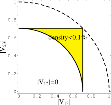
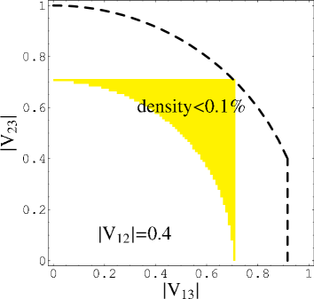
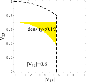
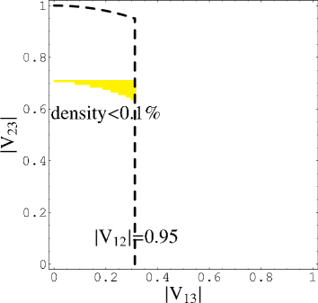
Figure 4: Region in the $|(V_{R})_{13}|-|(V_{R})_{23}|$ plane which gives $m_{3}/m_{2}\leq 6$ for some choice of the phases of $V_{R}$ (see eq.(14)). The yellow color indicates that in that region only less than 0.1% of the choices are successful. The scenario is defined by $M_{1}=M_{2}=M_{3}$ and $y_{1}:y_{2}:y_{3}=1:300:9\times 10^{4}$. Each plot corresponds to a different value of $|(V_{R})_{12}|$. The dashed line is the limit of unitarity of $V_{R}$, while the solid line in the first plot corresponds to the approximate analytical bound discussed at eq.(76).

It is worth mentioning that in this case a CKM-like form for $V_{R}$ cannot lead to a realistic spectrum, since [for any choice of the phases in eq.(14)] it is not consistent with a cancellation in the r.h.s. of eq.(75). However, it is funny that a MNS-like form can work correctly. More precisely, when $|(V_{R})_{13}|\ll 1$, as is the MNS case, the condition for cancellation in eq.(75) is approximately $|(V_{R})_{13}|^{2}\pm(|(V_{R})_{23}|^{2}-|(V_{R})_{33}|^{2})\simeq 0$. In terms of the parametrization (14), this reads

$$\tan^{2}\theta_{13}^{R}\simeq|\cos 2\theta_{23}^{R}|\ .$$ (77)

This condition is precisely fulfilled by an MNS-like matrix, thanks to the smallness of $\theta_{13}$ and the near-to-maximal $\theta_{23}$.

5 A suggestive ansatz

In sect. 4 we have not made any particular assumption about the (high-energy) parameters of the see-saw, apart from considering hierarchical neutrino Yukawa couplings, similar to those of quarks and charged leptons. Nevertheless, we showed that if the right-handed neutrino masses are hierarchical, a CKM-pattern for $V_{R}$ was naturally preferred in order to reproduce the experimental ratio between the two heavier neutrinos, $h={\kappa_{3}/\kappa_{2}}\lower 3.01385pt\hbox{$\;\stackrel{{\scriptstyle\textstyle<}}{{\sim}}\;$}6$, which is the only experimental constraint on ratios of neutrino masses. Similarly, we saw that if the right-handed neutrino masses are approximately degenerate, an MNS-like pattern for $V_{R}$ could equally work, but always with a certain fine-tuning. In this section we study more in deep these suggestive coincidences.

${\bf V_{R}=V_{\rm{\bf CKM}}}$ ansatz

We start by considering the possibility that $V_{R}$ coincides with the CKM matrix, $V_{\rm CKM}$. From eq.(14) $V_{R}$ has two phases, $\alpha_{1},\alpha_{2}$, that, unlike the quark CKM matrix, cannot be absorbed into redefinitions of the fields. Thus, the identification of $V_{R}$ with $V_{\rm CKM}$ has to be up to these two independent phases,

$$V_{R}={\rm diag}\left(e^{i\alpha_{1}},\ e^{i\alpha_{2}},\ 1\right)V_{\rm CKM}$$ (78)

This identification of $V_{R}$ with $V_{\rm CKM}$ evokes the $SU(5)$ connection between the $V_{L}$ mixing matrix for $d-$quarks and the $V_{R}$ one for charged leptons, which comes from the relation ${\bf Y}_{d}={\bf Y}_{l}^{T}$ between the corresponding Yukawa matrices. Following this analogy, we can make the ansatz that the eigenvalues of neutrino Yukawa couplings, $\{y_{1},y_{2},y_{3}\}$, coincide with the $u-$quark ones, $\{y_{u},y_{c},y_{t}\}$. We are not considering a definite GUT framework to justify this assumption (although it could proceed e.g. from some $SO(10)$ construction), but only exploring if it can work in practice, which is certainly non-trivial.

The first step to probe this ansatz is to write both $V_{\rm CKM}$ and $\{y_{u},y_{c},y_{t}\}$ at the scale of right-handed masses, $M\sim 10^{13}$ GeV, where the see-saw mechanism takes place and the identification (78) should be done. In the SM the RG change in the ratios $m_{u}:m_{c}:m_{t}=y_{u}:y_{c}:y_{t}$ from low- to high-energy is

$$y_{u}:y_{c}:y_{t}\ = \ 1.3\times 10^{-5}:7.1\times 10^{-3}:1\;\;\;{\rm at\ low\ scale}$$

$$\rightarrow\ y_{u}:y_{c}:y_{t}\ = \ 1.1\times 10^{-5}:3.2\times 10^{-3}:1\;\;\;{\rm at\ high\ scale}\$$ (79)

Note that the RGE change considerably the hierarchy of $u-$quarks (which, incidentally, becomes remarkably regular, on top of strong ). This is due mainly to the important effect of the top Yukawa coupling. On the other hand, the RGE for the neutrino mass matrix below the $M-$scale is flavour-blind, except for small effects proportional to the squared of the tau Yukawa coupling. This produces very small effects in the hierarchy of neutrino masses and in the MNS matrix (which we are not considering here anyhow), especially in the case of a soft hierarchy [11]. Thus we can neglect here the RGE effects for the neutrino sector. $V_{\rm CKM}$ undergoes a certain change as well for the same reasons. In magnitude,

$$\left|V_{\rm CKM}\right|\simeq\pmatrix{0.97&0.23&0.0043\cr&&\cr 0.23&0.973&0.042\cr&&\cr 0.008&0.04&1\cr}_{\rm low\ scale}\longrightarrow\ \ \pmatrix{0.97&0.23&0.0049\cr&&\cr 0.23&0.973&0.047\cr&&\cr 0.009&0.047&1\cr}_{\rm high\ scale}$$ (80)

The CP-phase, $\delta_{\rm CKM}\simeq 1$ rad, does not change appreciably along the running. Of course, eqs. (79, 80) have experimental errors. For our purposes the most significant ones are those associated to $(V_{\rm CKM})_{13}$ and $(V_{\rm CKM})_{23}$. Using the most recent analyses [3] and running consistently the quoted errors up to the $M-$scale [13, 14], we get $(V_{\rm CKM})_{13}=(4.9\pm 0.3)\times 10^{-3}$, $(V_{\rm CKM})_{23}=(47\pm 0.7)\times 10^{-3}$.

In addition we will consider, as mentioned, hierarchical right-handed masses, choosing a hierarchy equal to that of the Yukawa couplings. This is of course a somewhat arbitrary choice, but we find it simple and reasonable, and it does not amount to any extra assumption for a different hierarchy.

In summary, we will make the assumption

$$y_{1}:y_{2}:y_{3} = M_{1}:M_{2}:M_{3}\ =\ 1.1\times 10^{-5}:3.2\times 10^{-3}:1$$

$$V_{R} = {\rm diag}\left(e^{i\alpha_{1}},\ e^{i\alpha_{2}},\ 1\right)V_{\rm CKM}(M)$$ (81)

where $V_{\rm CKM}(M)$ is essentially given by (80).

Notice from (27, 26) that choosing $V_{R}={\bf 1}$ we would get a hierarchy of neutrino masses equal to that of Yukawa couplings, i.e. $h=\kappa_{3}/\kappa_{2}\sim 300$ [see eq.(5)]. This would be completely inconsistent with the experimental $h=\kappa_{3}/\kappa_{2}\lower 3.01385pt\hbox{$\;\stackrel{{\scriptstyle\textstyle<}}{{\sim}}\;$}6$, by a factor of 50. On the other hand, as is clear from the discussion around eq.(57), a random $V_{R}$ would give $h={\cal O}(10^{7})$, i.e. orders of magnitude away from the experimental range. Therefore, it is certainly non-trivial that the assumption (5) could be consistent with the experiment.

To illustrate these facts and show the results, we give in Fig.5, upper plots, the allowed region in the $|(V_{R})_{13}|-|(V_{R})_{23}|$ plane for fixed $|(V_{R})_{12}|=|(V_{\rm CKM})_{12}|$. Again, for each point we have evaluated $h=\kappa_{3}/\kappa_{2}$ for 1000 random values of the $\alpha_{1}$, $\alpha_{2}$ phases in $V_{R}$ ($\delta_{R}$ is fixed at $\delta_{\rm CKM}$), and counted the number of points that are compatible with the observed hierarchy, $h\lower 3.01385pt\hbox{$\;\stackrel{{\scriptstyle\textstyle<}}{{\sim}}\;$}6$. White areas are excluded, while colored areas are allowed. As expected only a tiny part of $\{|(V_{R})_{13}|,|(V_{R})_{23}|\}$ values are allowed [a good analytical approximation of the size and shape of the allowed region is given by (73)]. Remarkably, the CKM value for these quantities (represented by the cross in the figure) falls inside the allowed region, which we find very suggestive and highly non-trivial. Notice also that $V_{\rm CKM}$ is the only experimentally known example of a mixing matrix for Yukawas, as $V_{R}$ is ($V_{\rm MNS}$ is not, unless neutrinos are pure Dirac). All this makes the success of the CKM ansatz even more remarkable. It would be certainly nice to construct models (maybe in the GUT framework) to accommodate this “CKM-ansatz”.

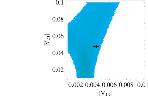
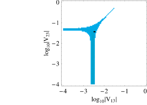
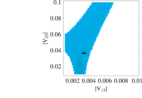
Figure 5: Region in the $|(V_{R})_{13}|-|(V_{R})_{23}|$ plane which, for $|(V_{R})_{12}|=|(V_{\rm CKM})_{12}|$, $\delta_{R}=\delta_{\rm CKM}$, and some choice of the $\alpha_{1}$, $\alpha_{2}$ phases (see eq.(14)), gives $m_{3}/m_{2}\leq 6$. The Yukawa couplings, $y_{i}$, and right-handed masses, $M_{i}$, are taken as indicated at eq.(5). The cross corresponds to the CKM values for $|(V_{R})_{13}|$, $|(V_{R})_{23}|$ (within experimental uncertainties). The upper (lower) plots correspond to the SM (SUSY) case. The color code is as in Fig. 3.

In order to gain analytical understanding for the success of the “CKM-ansatz” it is convenient to use the Wolfenstein parametrization of the CKM matrix:

$$V_{CKM}=\pmatrix{1-{\displaystyle{\lambda^{2}\over 2}}&\lambda&A\lambda^{3}(\rho-i\eta)\cr&&\cr-\lambda&1-{\displaystyle{\lambda^{2}\over 2}}&A\lambda^{2}\cr&&\cr A\lambda^{3}(1-\rho-i\eta)&-A\lambda^{2}&1\cr}+{\cal O}(\lambda^{4}),$$ (82)

where $\lambda$ is determined with a very good precision in semileptonic $K$ decays, giving $\lambda\simeq 0.23$, and $A$ is measured in semileptonic $B$ decays, giving $A\simeq 0.82$. The parameters $\rho$ and $\eta$ are more poorly measured, although a rough estimate is $\rho\simeq 0.1$, $\eta\simeq 0.3$ [12] (therefore $(\rho-i\eta)\simeq 0.3e^{i\delta}$, which is fairly close to $\lambda$ in absolute value). At high energies, only the parameter $A$ changes substantially [14], being $A\simeq 0.92$ at the scale $M\sim 10^{13}$GeV. Furthermore, we will use the following phenomenological relations among the up-type quark Yukawa couplings evaluated at high energies, that we assume also valid for the right-handed neutrino masses:

$$y_{1}:y_{2}:y_{3} \sim M_{1}:M_{2}:M_{3}\ \sim\ \lambda^{8}:\lambda^{4}:1$$ (83)

Substituting this ansatz in eq. (57) we obtain:

$$h={m_{3}\over m_{2}}\ \lower 3.01385pt\hbox{$\;\stackrel{{\scriptstyle\textstyle>}}{{\sim}}\;$}\ \lambda^{-6}\ \frac{\left|A^{2}(\rho-i\eta)^{2}e^{2i\alpha_{1}}+A^{2}\lambda^{2}e^{2i\alpha_{2}}+\lambda^{2}\right|^{2}}{\left|A^{2}(1-\rho-i\eta)^{2}+1+\lambda^{2}e^{2i\alpha_{2}}\right|}\sim{\cal O}(\lambda^{-2})$$ (84)

It is already remarkable the large reduction of the hierarchy that results just from the peculiar pattern of $V_{\rm CKM}$ (without taking into account the values of $\alpha_{1}$, $\alpha_{2}$): for random $V_{R}$, the natural size of the hierarchy is dictated by the ${y_{3}^{2}\over y_{2}^{2}}{M_{2}\over M_{1}}\sim\lambda^{-12}$ factor in eq. (57). Now, thanks to the structure of $V_{\rm CKM}$ given in eq.(82), the second factor in eq. (57) (i.e. the fraction of absolute values) gets ${\cal O}(\lambda^{10})$, leading to (84). Plugging numbers, for random $\alpha_{1}$, $\alpha_{2}$, this amounts to a reduction from $h\sim{\cal O}(10^{7})$ to $h\sim 100$. This is still too large compared to $h^{\rm exp}\sim 6$, but shows that $V_{\rm CKM}$ does soften $h$ in an extremely efficient way. Choosing $\alpha_{1}-\delta\sim{\pi\over 2},{3\pi\over 2}$ and $\alpha_{2}\sim 0,\pi$ the numerator of eq. (84) gets much smaller due to a cancellation among the three terms. This is possible thanks to the fact that the three terms have similar magnitude, which is a fortunate coincidence (changing $V_{R}$, even keeping the same pattern, this fact generally disappears). Then we get $h={\cal O}(1)$, i.e. consistent with the experiment. This choice of phases is as good as any other else, implying that there is no need of fine tuning of the phases to get the desired result.

Coming back to the numerical computation, the previous arguments are illustrated in Fig.6, left plot, which shows the region of experimentally acceptable values of $h$ in the $\alpha_{1}-\alpha_{2}$ plane. More precisely, the green area corresponds to $5.5\leq h\leq 6$, which is the experimental $1-\sigma$ value of $h^{exp}$ when $m_{2}/m_{1}\gg 1$ (see Fig. 1), as is the case. As noted above this allowed region replicates with periodicity $\pi$. All the remaining parameters of $V_{R}$ have been taken at the central values of $V_{\rm CKM}$. Clearly, the allowed region for $\alpha_{1}$, $\alpha_{2}$ is quite “macroscopic”, i.e. it is not fine-tuned. In fact, the minimal value for $h$ is close to the experimental value $h\sim 6$ (note that since $\kappa_{1}$ is hierarchically smaller, as will be commented shortly, the value of $h$ must be close to its experimental upper bound). This is funny since the region of minimal values of $h$ is naturally enhanced in size (near a minimum the function changes little).

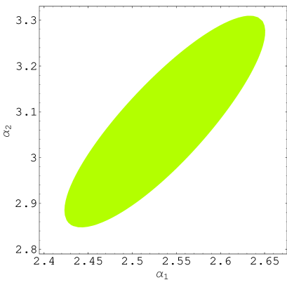
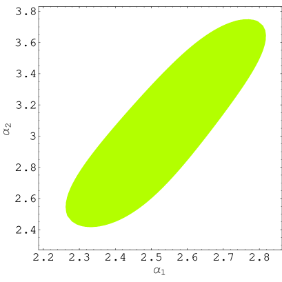
Figure 6: Region of the $\alpha_{1}-\alpha_{2}$ plane that gives values of $m_{3}/m_{2}$ consistent with the experiment for all the remaining parameters of $V_{R}$ (see Right and left plots correspond to the SM and SUSY cases respectively. Note the different scales of the two plots.

Let us indicate that the mass of the lightest neutrino, $\kappa_{1}$, becomes orders of magnitude smaller than $\kappa_{2}$, in agreement with the general results of sect. 4.3 (see the discussion after eq.[68)]. To be precise, the value of the lightest neutrino mass predicted by this ansatz is

$$m_{1}=v\kappa_{1}\simeq 3\times 10^{-6}m_{2}=3\times 10^{-8}{\rm eV}$$ (85)

The SUSY case works in a similar way. The main difference are the RGEs, which are a bit different and, besides, depend on the value of $\tan\beta$, though not dramatically. The results for the CKM ansatz are also similar, and even better, as shown in Fig. 5 (lower plots) and Fig. 6 (right plot) for a typical case ($\tan\beta=10$).

Finally, let us mention that choosing a hierarchy for the Yukawa couplings as that of $d-$quarks (which is quite milder) enhances the allowed region in the $|(V_{R})_{13}|-|(V_{R})_{23}|$ plane. Then the CKM point continues to fall inside the allowed region.

${\bf V_{R}=V_{\rm{\bf MNS}}}$ ansatz

Let us now consider the $V_{R}\sim V_{\rm{\bf MNS}}$ possibility. As discussed at the end of subsect.4.3, this can work if the right-handed masses are quasi-degenerate; for simplicity we will assume $M_{1}=M_{2}=M_{3}$. As for the CKM case, the identification of $V_{\rm{\bf MNS}}$ and $V_{R}$ can only be made up to the two independent $\alpha_{1}$, $\alpha_{2}$ phases in (14). The Majorana phases of $V_{\rm{\bf MNS}}$ act from the opposite side, see eq.(7), and cannot be identified with $\alpha_{1}$, $\alpha_{2}$. In any case, we do not have any experimental information about these Majorana phases, nor about $\delta$, in the MNS matrix. So we take

$$V_{R}={\rm diag}\left(e^{i\alpha_{1}},\ e^{i\alpha_{2}},\ 1\right)V$$ (86)

where $V$ is the “non-Majorana” part of the MNS matrix, given in eq.(8). More precisely [2],

$$\sin^{2}\theta_{12}=0.26-0.36,\;\;\;\;\sin^{2}\theta_{23}=0.38-0.63,\;\;\;\;\sin^{2}\theta_{13}\leq 0.025,$$ (87)

the value of $\delta$ is left free. Concerning Yukawa couplings, as in the CKM case we identify them with the $u$–quark Yukawa couplings at high energy, which for the SM are given in eq.(79).

The results are given in Fig.7, left plot, which shows the allowed region in the $|(V_{R})_{13}|-|(V_{R})_{23}|$ plane for fixed $|(V_{R})_{12}|=|(V_{\rm MNS})_{12}|$. Again, colored areas are consistent (for some choice of the phases) with the observed hierarchy, $h\lower 3.01385pt\hbox{$\;\stackrel{{\scriptstyle\textstyle<}}{{\sim}}\;$}6$, while white areas are excluded. The MNS value for $|(V_{R})_{13}|,\ |(V_{R})_{23}|$ is represented by a cross in the figure, falling inside the allowed region.

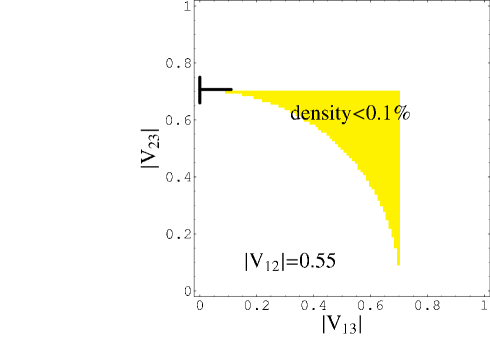
Figure 7: The same as Fig. 5 but for $V_{\rm CKM}\rightarrow V_{\rm MNS}$ and taking $M_{1}=M_{2}=M_{3}$. The $\delta_{\rm MNS}$ phase is left free, since it is experimentally unknown. The left (right) plot corresponds to the SM (SUSY) case. The color code is as in Fig. 4.

Although this is perhaps less suggestive than the good performance of $V_{\rm CKM}$ in the case of hierarchical right-handed masses, it is still quite remarkable. Concerning the values of the phases that do the job, it is clear from (75) that the necessary cancellation inside the straight brackets requires in this case $\alpha_{2}\simeq\pm i\pi$, since $(V_{R})_{13}^{2}\simeq 0$. The previous cancellation must be quite fine as can be seen noting that the ratio of squared Yukawa couplings in the right hand side of (75) is $\sim 10^{5}$, so the $|\ |^{2}$ factor must be very small in order to obtain $h\simeq 6$ (a tunning of $\lower 3.01385pt\hbox{$\;\stackrel{{\scriptstyle\textstyle<}}{{\sim}}\;$}1\%$ is needed).

The performance of the SUSY case is similar, as shown in Fig. 7, right plot.

6 Summary and conclusions

In this paper we have started from the fact that the observed mass ratio for the two heavier low-energy neutrinos, $h=m_{3}/m_{2}\lower 3.01385pt\hbox{$\;\stackrel{{\scriptstyle\textstyle<}}{{\sim}}\;$}6$, is much smaller than the corresponding ratios observed for quarks and charged leptons, which are ${\cal O}(20)$ or ${\cal O}(300)$ (for the other independent neutrino mass ratio, $m_{2}/m_{1}$, there is no experimental constraint). We have wondered whether this peculiar pattern of neutrino masses can be a consequence of the peculiar way they are generated through a see-saw mechanism, investigating how the present experimental data restrict the structure of the high-energy seesaw parameters and which choices, among the allowed ones, produce more naturally the observed pattern of neutrino masses. We have studied in particular (but not only) if starting with hierarchical neutrino Yukawa couplings, as for the other fermions, one can naturally get the observed $m_{3}/m_{2}\lower 3.01385pt\hbox{$\;\stackrel{{\scriptstyle\textstyle<}}{{\sim}}\;$}6$ ratio.

To perform this analysis we have first put forward a top-down parametrization of the see-saw mechanism in terms of (high-energy) basis-independent quantities: the Yukawa and right-handed-mass ”eigenvalues”, $\{y_{i},M_{i}\}$, and two unitary matrices, $V_{L},V_{R}$, associated to the diagonalization of the Yukawa matrix, as shown in eqs.(12, 13). From these 18 independent parameters, we have shown that the neutrino mass eigenvalues depend just on 12 of them: $\{y_{i},M_{i}\}$ and $V_{R}$, which simplifies the analysis a lot. On the other hand, $V_{L}$ can be derived from the other parameters and $V_{\rm MNS}$. This is summarized in eqs.(23, 26–28). A parametrization of $V_{R}$ is given in (14).

In our analysis (which is valid for both the SM and the SUSY versions of the see-saw) we have made an extensive use of some analytical inequalities satisfied by the eigenvalues of a general hermitian matrix. This allows to obtain very simple expressions that describe faithfully the exact results and permit to gain intuition on the problem, e.g. the useful lower bound on $h$ given by eq.(57). This analytical study was complemented by a numerical and statistical survey, in order to obtain and present accurate results.

Our main conclusions are the following:

• For random values of the $V_{R}$ entries we expect a low-energy neutrino hierarchy $h={m_{3}\over m_{2}}\lower 3.01385pt\hbox{$\;\stackrel{{\scriptstyle\textstyle>}}{{\sim}}\;$}\ {y_{3}^{2}\over y_{2}^{2}}{M_{2}\over M_{1}}$. If the Yukawa couplings are hierarchical, similarly to the other fermions, then we expect $h$ orders of magnitude larger than the experimental value and the hierarchy of Yukawas itself. So, either we give up the natural assumption that the neutrino Yukawa couplings present a hierarchy similar to other fermions, or we accept that the $V_{R}$ entries are far from random. In the second case the structure of $V_{R}$ becomes strongly constrained. In particular, from eq.(57), $\left|(V_{R})_{13}^{2}+{M_{1}\over M_{2}}(V_{R})_{23}^{2}+{M_{1}\over M_{3}}(V_{R})_{33}^{2}\right|^{2}\ll 1$ is required, and $(V_{R})_{12}$ sizeable is desirable.

• If we keep the assumption of hierarchical neutrino Yukawa couplings, a low-energy spectrum of quasi-degeneracy or soft hierarchy for the three neutrinos requires either $M_{i}/M_{j}\simeq y_{i}^{2}/y_{j}^{2}$, $V_{R}\simeq{\bf 1}$, or a very delicate tuning between $\{y_{i},M_{i}\}$ and $V_{R}$. In the absence of an explanation for this strong fine-tuning we consider this scenario as unnatural.

• On the other hand, if we just attempt to reproduce the only experimentally constrained mass ratio, $h=m_{3}/m_{2}\lower 3.01385pt\hbox{$\;\stackrel{{\scriptstyle\textstyle<}}{{\sim}}\;$}6$, the prospects are much more interesting: a characteristic pattern for the $V_{R}$ matrix emerges, but there is no need of fine-tuning between the parameters.

  • If the right-handed neutrino masses are hierarchical, $M_{1}\ll M_{2}\ll M_{3}$, the selected pattern for $V_{R}$ is characterized by very small $|(V_{R})_{13}|$, $|(V_{R})_{23}|$, and sizeable $|(V_{R})_{21}|$, which remarkably resembles the structure of the CKM matrix. (actually the discussion before eq.(69) suggests $|(V_{R})_{13}|^{2}\ll|(V_{R})_{23}|^{2}$, also in coincidence with CKM).

  • If the right-handed neutrino masses are degenerate, $M_{1}\simeq M_{2}\simeq M_{3}$, it is not possible to reproduce $h^{\rm exp}$ without a certain fine-tuning. The selected form for $V_{R}$ is not compatible with $V_{\rm CKM}$, but, quite amusingly, it is with $V_{\rm MNS}$ (altough, in this case, other patterns for $V_{R}$ very different from $V_{\rm MNS}$ work as well).

  In all the cases, the mass of the lightest neutrino, $m_{1}$, is naturally orders of magnitude smaller than $m_{2}$, which comes out as a natural prediction of a scenario with hierarchical neutrino Yukawa couplings.

• Motivated by the previous coincidences we have explicitely checked that identifying $V_{R}$ with $V_{\rm CKM}$ and taking a hierarchy of neutrino Yukawa couplings (and right-handed masses) equal to that of the $u-$quarks, gives $h$ consistent with the experimental limit, $h^{\rm exp}\lower 3.01385pt\hbox{$\;\stackrel{{\scriptstyle\textstyle<}}{{\sim}}\;$}6$. This is highly non-trivial since $V_{R}={\bf 1}$ gives $h\simeq 300$ and a random $V_{R}$ typically gives $h={\cal O}(10^{6})$. We have not attempted to construct a GUT model to accommodate this suggestive feature, but it might be an interesting line of work. For the SUSY case there are slight differences coming from the form of the RGE, but the results are very similar (and even better).

  Likewise using $V_{\rm MNS}$ in the same context, but with degenerate right-handed neutrino masses, is also consistent with the experiment.

7 Outlook

The fact that $V_{R}$ is very constrained once a hierarchical structure for the Yukawas is assumed, has an important impact on several physical issues.

Constraints from ${\bf U_{\rm MNS}}$

We have explored the constraints on $V_{R}$ from the peculiar pattern of physical neutrino masses. Similarly, the experimental $U_{\rm MNS}$ may constrain the high-energy parameters. Although we have seen, eq.(28), that $V_{L}$ can always be adjusted to give the observed $U_{\rm MNS}$, it is not guaranteed that such choice is without tunings for all the possible $V_{R}$. This may shed additional light on the structure of the high-energy theory.

Relation to the $R$–parametrization

The connection of the botton-up parametrization (24), based on an orthogonal complex matrix $R$ and the top-down parametrization (26–28), based on the $V_{R}$ matrix, is given in (31). Nevertheless, it would be very helpful for phenomenological studies to determine from the beginning the form of $R$ consistent with e.g. hierarchical neutrino Yukawa couplings. This would give an indication about which $R$s are more natural, and would make easier in general the exploration of phenomenological signatures of top-down assumptions.

Leptogenesis

If one ignores flavour effects, the rate of leptogenesis produced by the decay of the right-handed neutrinos is proportional to particular entries of the matrix

$$YY^{\dagger}=V_{R}D_{Y^{2}}V_{R}^{\dagger}\ .$$ (88)

where $D_{Y^{2}}={\rm diag}\{y_{1}^{2},y_{2}^{2},y_{3}^{2}\}$. Since the assumption of hierarchical $y_{i}$ strongly constrains $V_{R}$, the corresponding results for leptogenesis are directly affected.

For the two-neutrino case (see sect. 3), the implications are particularly nitid: the CP Majorana phase of $V_{R}$ (the only source of CP violation for this issue) must be close to a CP-conserving value, which would make the leptogenesis process inefficient. Nevertheless, flavour effects can rescue this scenario when the temperature at which leptogenesis takes place is smaller than $\sim 10^{12}$GeV, as was shown in [15] (note that this scenario would correspond to the case $R$ real). The analysis for three neutrinos is a bit more involved but it has an obvious interest.

In a supersymmetric framework, another mechanism to generate the observed baryon asymmetry is Affleck-Dine leptogenesis [16]. Thermal effects and gravitino overproduction constrain the smallest neutrino mass to be $m_{1}\lower 3.01385pt\hbox{$\;\stackrel{{\scriptstyle\textstyle<}}{{\sim}}\;$}10^{-8}$eV [17]. Despite the large hierarchy between $m_{2}$ and $m_{1}$ might seem a priory unnaturally strong, we have shown that it is in fact a prediction of the see-saw mechanism with the suggestive ansatz proposed in section 5 [see eq.(85)].

Rare LFV processes

In the context of SUSY, it is well known that even starting with universal soft masses at high energy, one ends up with flavour-violating entries in the mass-matrices, mainly due to the effect of the neutrino Yukawa couplings in the running between the high-energy scale ($M_{p}$ in the gravity-mediated case) and the scale of the right-handed masses [18]. Such effect is proportional to

$$Y^{\dagger}Y=V_{L}D_{Y^{2}}V_{L}^{\dagger}\ .$$ (89)

Although $V_{L}$ is not directly constrained from the low-energy spectrum, once $V_{R}$ is determined, $V_{L}$ is obtained from eq.(28). The corresponding rates for LFV processes, such as $\mu\rightarrow e,\gamma$, may constrain further the scenario and offer predictions for present and future experiments.

GUT constructions

As mentioned above, identifying $V_{R}$ with $V_{\rm CKM}$ and taking a hierarchy of neutrino Yukawa couplings (and right-handed masses) equal to that of the $u-$quarks, is (non-trivially) consistent with the experiment. It would be very interesting to build a GUT model able to accommodate this appealing feature.

Anarchic neutrinos

As mentioned at the end of subsect. 4.1, the basis-independent top-down parametrization of the see-saw mechanism that we have used is likely very appropriate to study scenarios of anarchic neutrinos [9], since these are based on statistical considerations about the high-energy parameters that define the theory, and it is highly desirable that these parameters are basis-independent. We gave there a simple example of how such analysis can be, but clearly much work could be done in this direction.

——————

Work along the above lines is currently in progress.

Appendix

Here we summarize some useful formulas concerning the eigenvalues of a (general or not) matrix.

According to the Gershgorin Circle Theorem, every eigenvalue of any complex $n\times n$ matrix $A$ lies within at least one of the $n$ Gershgorin discs defined as

$$D(A_{ii},R_{i})\equiv\{z:|z-A_{ii}|\leq R_{i}\}\ .$$ (90)

where $R_{i}$ is the Gershgorin radius of the Gershgorin disc centered at $A_{ii}$,

$$R_{i}=\sum_{j\neq i}\left|A_{ij}\right|\ .$$ (91)

For the proof, let $\lambda$ be an eigenvalue of $A$ with eigenvector ${\bf v}\equiv\{v_{j}\}$. Define $|v_{i}|={\rm max}_{j}|v_{j}|$ (always $|v_{i}|>0$). Then the eigenvalue equation $A{\bf v}=\lambda{\bf v}$ can be written as

$$\lambda v_{i}-A_{ii}v_{i}=\sum_{j\neq i}A_{ij}v_{j}$$ (92)

Dividing both sides by $v_{i}$ and taking the norm we obtain

$$|\lambda-A_{ii}|=\left|\sum_{j\neq i}A_{ij}v_{j}/v_{i}\right|\leq\sum_{j\neq i}|A_{ij}|=R_{i}$$ (93)

Working with $A^{T}$ instead of $A$ we get an analogous expression for the same eigenvalues changing $R_{i}\rightarrow\sum_{j\neq i}|A_{ji}|$. I.e. for each diagonal element, there is one Gershgorin radius associated with the row and one with the column. Furthermore it can be shown that if the $n$ discs can be partitioned into disjoint subsets of the complex plane then each subset contains the same number of eigenvalues as discs.

If the original matrix $A$ is hermitian, then the eigenvalues of $A$, say $\lambda_{i}$, and diagonal elements, $A_{ii}$, are real, so the discs become segments in the real line. Furthermore, the Gershgorin segments associated with the rows and the columns coincide.

All this can be applied to eq.(27). In particular, for the case of three neutrinos with hierarchical Yukawa couplings, $y_{1}\ll y_{2}\ll y_{3}$, the diagonal entry $\left(\kappa^{\prime}\kappa^{\prime\dagger}\right)_{33}$ is normally much larger than the others and the corresponding Gershgorin radius is much smaller (see below), so the Gershgorin disc is usually disjoint from the others. This means that the largest eigenvalue, $\kappa_{3}^{2}$, satisfies

$$\left|\kappa_{3}^{2}-\left(\kappa^{\prime}\kappa^{\prime\dagger}\right)_{33}\right|\leq\sum_{j\neq 3}\left|\left(\kappa^{\prime}\kappa^{\prime\dagger}\right)_{3j}\right|$$ (94)

which is similar to eq.(51) [note that the right-hand-side of eq.(94), i.e. the Gershgorin radius, is supressed by a ${y_{2}\over y_{3}}-$factor with respect to $\left(\kappa^{\prime}\kappa^{\prime\dagger}\right)_{33}$].

Analogous inequalities can be produced for $\kappa_{1}^{2}$. In this case, the most efficient ones come from considering the inverse matrix, $\kappa^{\prime-1}(\kappa^{\prime-1})^{\dagger}$, which is a positive hermitian matrix with $\kappa_{i}^{-2}$ eigenvalues.

The inequalities for $\kappa_{3}$, $\kappa_{1}$ produced in this way can be plugged into (49) to give bounds on $h$ similar to those considered in sect. 4.

Let us recall that in that section we found more efficient for the sake of clarity to use the fact that in a positive hermitian matrix, such as $\kappa^{\prime}\kappa^{\prime\dagger}$ and $\kappa^{\prime-1}(\kappa^{\prime-1})^{\dagger}$, the largest eigenvalue ($\kappa_{3}^{2}$ and $\kappa_{1}^{-2}$ respectively) must be larger than any diagonal entry of the matrix.

For the proof, let $A$ be a positive hermitian $n\times n$ matrix with eigenvalues $\{\lambda_{i}\}$ and eigenvectors $\{{\bf v_{i}}\}$, ordered as $\lambda_{1}\leq\lambda_{2}\leq\cdots\lambda_{n}$. Writing the normalized vector in the $i^{\rm th}$-direction, ${\bf e_{i}}$, as ${\bf e_{i}}=\sum a_{ij}{\bf v_{j}}$ with $\sum|a_{ij}|^{2}=1$, then

$${\bf e_{i}}^{\dagger}A{\bf e_{i}}=A_{ii}=\sum\lambda_{j}|a_{ij}|^{2}\leq\lambda_{n}$$ (95)

Similarly it can be shown that $\lambda_{1}\leq A_{ii}$ (for any $i$). The above lower bound for $\lambda_{n}$ is complemented with the obvious upper bound $\lambda_{n}\leq{\rm tr}A$. This allows to corner the range of values where $\lambda_{n}$ lies. (This procedure is very efficient for $\kappa^{\prime}\kappa^{\prime\dagger}$ and $\kappa^{\prime-1}(\kappa^{\prime-1})^{\dagger}$, since the trace is strongly dominated by the largest diagonal entry.)

These inequalities can be made stronger replacing $A_{ii}$ by the eigenvalues of any $m\times m$ submatrix of $A$ (with $m\leq n$). This can be seen by diagonalizing the submatrix with $A^{\prime}=V^{\dagger}AV$, where $V$ is a unitary matrix which is trivial except in the corresponding $m\times m$ box, and then applying the same argument to $A^{\prime}$.

All these kinds of inequalities can be plugged into (49) to obtain alternative bounds on $h$. Also they can be used to put bounds on the ratio $\kappa_{3}/\kappa_{1}$, which gives a direct measure of how far is the neutrino spectrum from the exactly degenerate case.

References

- [1] For a review on neutrino physics, see M. C. Gonzalez-Garcia and Y. Nir, Rev. Mod. Phys. 75 (2003) 345 [arXiv:hep-ph/0202058].
- [2] M. Maltoni, T. Schwetz, M. A. Tortola and J. W. F. Valle, New J. Phys. 6 (2004) 122 [arXiv:hep-ph/0405172]. (Updated June–2006)
- [3] W. M. Yao et al. [Particle Data Group], J. Phys. G 33 (2006) 1.
- [4] P. Minkowski, Phys. Lett. B 67 (1977) 421. M. Gell-Mann, P. Ramond and R. Slansky, Proceedings of the Supergravity Stony Brook Workshop, New York 1979, eds. P. Van Nieuwenhuizen and D. Freedman; T. Yanagida, Proceedinds of the Workshop on Unified Theories and Baryon Number in the Universe, Tsukuba, Japan 1979, eds. A. Sawada and A. Sugamoto; R. N. Mohapatra, G. Senjanovic, Phys.Rev.Lett. 44 (1980)912, ibid. Phys.Rev. D23 (1981) 165; S. L. Glashow, The Future Of Elementary Particle Physics, In *Cargese 1979, Proceedings, Quarks and Leptons*, 687-713 and Harvard Univ.Cambridge - HUTP-79-A059 (79,REC.DEC.) 40p.
- [5] S. Pascoli, S. T. Petcov and W. Rodejohann, LFV Phys. Rev. D 68 (2003) 093007 [arXiv:hep-ph/0302054].
- [6] J. A. Casas and A. Ibarra, Nucl. Phys. B 618 (2001) 171 [arXiv:hep-ph/0103065].
- [7] A. Broncano, M. B. Gavela and E. Jenkins, Nucl. Phys. B 672 (2003) 163 [arXiv:hep-ph/0307058].; S. F. King, arXiv:hep-ph/0610239; S. Antusch and S. F. King, JHEP 0601 (2006) 117 [arXiv:hep-ph/0507333].
- [8] P. H. Frampton, S. L. Glashow and T. Yanagida, Phys. Lett. B 548 (2002) 119 [arXiv:hep-ph/0208157]; M. Raidal and A. Strumia, Phys. Lett. B 553 (2003) 72 [arXiv:hep-ph/0210021]; A. Ibarra and G. G. Ross, Phys. Lett. B 591 (2004) 285 [arXiv:hep-ph/0312138]; W. l. Guo, Z. z. Xing and S. Zhou, arXiv:hep-ph/0612033.
- [9] L. J. Hall, H. Murayama and N. Weiner, Phys. Rev. Lett. 84 (2000) 2572 [arXiv:hep-ph/9911341]; N. Haba and H. Murayama, Phys. Rev. D 63 (2001) 053010 [arXiv:hep-ph/0009174]; A. de Gouvea and H. Murayama, Phys. Lett. B 573 (2003) 94 [arXiv:hep-ph/0301050]; J. R. Espinosa, arXiv:hep-ph/0306019.
- [10] L. Everett and P. Ramond, arXiv:hep-ph/0608069.
- [11] J. A. Casas, J. R. Espinosa, A. Ibarra and I. Navarro, Nucl. Phys. B 573 (2000) 652 [arXiv:hep-ph/9910420].
- [12] See, for instance, M. Battaglia et al., “The CKM matrix and the unitarity triangle,” [hep-ph/0304132].
- [13] M. Olechowski and S. Pokorski, Phys. Lett. B 257 (1991) 388.
- [14] P. Ramond, R. G. Roberts and G. G. Ross, Nucl. Phys. B 406 (1993) 19 [arXiv:hep-ph/9303320].
- [15] A. Abada, S. Davidson, F. X. Josse-Michaux, M. Losada and A. Riotto, JCAP 0604, 004 (2006) [arXiv:hep-ph/0601083]; E. Nardi, Y. Nir, E. Roulet and J. Racker, JHEP 0601, 164 (2006) [arXiv:hep-ph/0601084]; A. Abada, S. Davidson, A. Ibarra, F. X. Josse-Michaux, M. Losada and A. Riotto, JHEP 0609, 010 (2006) [arXiv:hep-ph/0605281].
- [16] I. Affleck and M. Dine, Nucl. Phys. B 249, 361 (1985).
- [17] T. Asaka, M. Fujii, K. Hamaguchi and T. Yanagida, Phys. Rev. D 62, 123514 (2000) [arXiv:hep-ph/0008041].
- [18] F. Borzumati and A. Masiero, Phys. Rev. Lett. 57, 961 (1986).