Angular ordering and parton showers for non-global QCD observables

Abstract:

We study the mismatch between a full calculation of non-global single-logarithms in the large-$N_{c}$ limit and an approximation based on free azimuthal averaging, and the consequent angular-ordered pattern of soft gluon radiation in QCD. We compare the results obtained in either case to those obtained from the parton showers in the Monte Carlo event generators HERWIG and PYTHIA, with the aim of assessing the accuracy of the parton showers with regard to such observables where angular ordering is merely an approximation even at leading-logarithmic accuracy and which are commonly employed for the tuning of event generators to data.

1 Introduction

An important class of theoretical predictions in QCD fall under the banner of “all-order” calculations. This refers specifically to predictions for those observables that receive logarithmic enhancements at each order of perturbation theory, which threaten the convergence of the perturbation expansion in important regions of phase space. A classic example is event-shape distributions, where studying an observable close to its Born value (such as the distribution of the thrust variable $1-T$ near $T=1$) results in generating terms as singular as $\alpha_{s}^{n}\frac{1}{1-T}\ln^{2n-1}(1-T)$ in the perturbative prediction, which can render all orders in $\alpha_{s}$ equally significant [1]. The origin of these logarithmic enhancements is the singular behaviour of the QCD emission probabilities and their virtual counterparts in the soft and/or collinear kinematical regions. These singularities coupled with the nature of the observable (where measuring close to the Born value constrains real emission but not the purely virtual terms) lead to the appearance of large uncancelled logarithmic contributions in the fixed-order perturbative results.

There exist two main approaches to deal with such logarithmic enhancements at all orders. The first is the method of analytical resummation where insight on the QCD multiple soft-collinear emission probabilities and analytical manipulations of the phase space constraints are carried out so as to obtain a result that resums the large logarithms (for those variables that satisfy certain conditions ensuring they can in fact be resummed [2]) into a function which can be expressed in the form

$$\Sigma(V)=\exp\left[Lg_{1}(\alpha_{s}L)+g_{2}(\alpha_{s}L)+\alpha_{s}g_{3}(\alpha_{s}L)+\cdots\right]\,,\qquad L\equiv\ln\frac{1}{V},$$ (1)

where $Lg_{1}$, $g_{2}$, etc. are functions that are computed analytically and $V$ is a generic event shape, e.g. $1-T$. The function $Lg_{1}$, if non-zero, represents the leading or double-logarithmic contribution (LL), since it contains an extra power of $L$ relative to the power of $\alpha_{s}$, i.e. ${\cal O}(\alpha_{s}^{n}L^{n+1})$. $g_{2}$ is the single-logarithmic or next-to-leading logarithmic (NLL) contribution containing a logarithm $L$ for each power of $\alpha_{s}$, ${\cal O}(\alpha_{s}^{n}L^{n})$, etc. We especially note that if the function $g_{1}$ is zero (as in the case of the interjet energy flow observable we shall study in detail here), the single-logarithmic function $g_{2}$ contains the leading logarithms. The function $\alpha_{s}g_{3}$ contains an extra power of $\alpha_{s}$ relative to the power of $L$ and is next-to–next-to leading logarithmic (NNLL) if $g_{1}$ is present and next-to–leading logarithmic (NLL) otherwise. In the limit $V\!\to 0$, $\Sigma(V)$ has a physical behaviour as opposed to its expansion to any fixed order, which is divergent as we mentioned. This expression, which is valid at small $V$, can then be matched to exact fixed-order estimates that account for the large-$V$ region, so as to give the best possible description over the entire range of $V$.

Another possible approach to studying such observables is provided by Monte Carlo event generators amongst which the most commonly employed are HERWIG [4, 5] and PYTHIA [6, 7, 8]. We note that these programs are of far greater general utility than the study of the observables we will discuss here, providing simulations of complete QCD events at hadron level and representing perhaps the most significant physics tools in current high-energy phenomenology. The parton showers contained in these event generators aim to capture at least the leading infrared and collinear singularities involved in the branching of partons, to all orders in the large-$N_{c}$ limit. One may thus expect that the dynamics that is represented by the parton shower ought to be similar to that which is used as analytical input in QCD resummations at least on the level of the leading (double) logarithms involved.

For several observables a correspondence between the Monte Carlo parton shower and the matrix elements used in analytical resummations is in fact clear. Considering, for example, final-state radiation, parton showers evolve due to parton emission with the branching probability $\mathcal{P}$ satisfying [9, 10, 11]

$$\frac{d{\mathcal{P}}}{d\ln k^{2}dz}=\frac{\alpha_{{\textsc{s}}}}{2\pi}\,P(z)\,\frac{\Delta(k^{2}_{\mathrm{max}},k_{0}^{2})}{\Delta(k^{2},k_{0}^{2})}\,,$$ (2)

where $k^{2}_{\max}$ is the maximum $k^{2}$ accessible to the branching and $k^{2}_{0}$ is a cut-off regularising soft and collinear singularities. The above result, with $P(z)$ being the appropriate Altarelli–Parisi splitting function relevant to the branching, captures the soft ($z\to 0$) and collinear ($k^{2}\to 0$) singularities of the emission. Virtual corrections (and hence unitarity) are incorporated via the Sudakov form factors $\Delta(k^{2},k_{0}^{2})$.

An essentially similar form is employed for the purposes of most analytical resummations where the probability of emitting several soft gluons is treated as independent emission of the gluons by the hard partons which for simplicity, in the rest of this paper, we take to be a $q\bar{q}$ pair. The probability for emitting a soft and/or collinear gluon is the very form mentioned above and the virtual corrections are included as in the Sudakov factor. This independent-emission or probabilistic pattern (which stems from the classical nature of soft radiation) suffices up to next-to–leading or single logarithmic accuracy for a large number of observables. Thus it is natural to expect that at least as far as the double-logarithmic function $g_{1}$ is concerned, it would be accurately contained within the parton shower approach, although it cannot be separated cleanly from the single-logarithmic and subleading effects generated by the shower. Beyond the double logarithmic level one expects at least a partial overlap between the parton shower and the analytical resummations, where the degree of overlap may vary from observable to observable and depend on which hard process one chooses to address. The state of the art of most analytical resummations is next-to–leading logarithmic, i.e. computing the full answer up to the function $g_{2}$. Monte Carlo algorithms such as HERWIG are certainly correct up to $g_{1}$ and perhaps in certain cases $g_{2}$ accuracy (while being limited to the large-$N_{c}$ approximation) but not beyond (see, e.g., the discussion in [12]).

As we mentioned, the event generator results do not explicitly separate leading logarithmic from next-to-leading logarithmic or subleading effects (e.g. those that give rise to $g_{3}$ and beyond) and, moreover, parton-level Monte Carlo results include non-perturbative effects that arise via the use of a shower cut-off scale, i.e. $k_{0}$ in Eq. (2). From the point of view of having a clean prediction valid to NLL accuracy that can be matched to fixed-order and supplemented by, for instance, analytically estimated power corrections, one would clearly prefer a resummed calculation. This is not a surprise since these calculations were developed keeping specific observables in mind unlike the event generators which have a much broader sweep and aim. It is thus not our aim to probe event generators as resummation tools in themselves but rather to consider the logarithmic accuracy to which perturbative radiation may be generically described by a parton shower of the kind to be found in HERWIG or PYTHIA, for different observables.

The above is particularly important since it has been pointed out relatively recently that for a large number of commonly studied observables, which are called non-global observables [13, 14], the approximation of independent emissions, used in the analytical resummations, is not valid to single (which for some of these observables means leading) logarithmic accuracy. Non-global observables typically involve measurements of soft emissions over a limited part of phase space, a good example being energy flow distributions in a fixed rapidity-azimuth ($\eta-\phi)$ region. In fact in the case of the energy flow away from hard jets the function $g_{1}$ in Eq. (1) is absent (there being no collinear enhancement in the away-from-jet region). The leading logarithms in this case are thus single logarithms that are resummed in a function equivalent to $g_{2}$ but this function cannot be completely calculated within an independent emission formalism. This is the case because the independent emission approximation of the QCD multi-parton emission pattern is strictly valid and intended for use in regions where successive emissions are strongly ordered in angle. The leading partonic configurations (those that give rise to the leading single-logarithms) for the away-from–jet energy flow are however those which include the region of emission angles of the same order in the parton cascade. Thus relevant single-logarithms also arise from multi-soft correlated emission which has been computed only numerically and in the large-$N_{c}$ limit thus far [13, 14, 15].

Since one of the main approximations used in analytical resummations, that of independent emission, has been shown to be inaccurate even to leading-logarithmic accuracy for some non-global observables like interjet energy flow, one is led to wonder about the leading-logarithmic accuracy that is claimed for parton showers in Monte Carlo event generators, in these instances. The parton shower in HERWIG for instance relies on an evolution variable $k^{2}$ which in the soft limit is equivalent to ordering in angle [11, 16]. Angular ordering of a soft partonic cascade, initiated by a hard leg, is a perfectly good approximation for azimuthally averaged quantities such as some $e^{+}e^{-}$ event shapes and in fact can be further reduced in these instances to an independent emission pattern, up to next-to–leading logarithmic accuracy. However, when looking at energy flow into limited angular intervals, one is no longer free to average soft emissions over the full range of angles, which means that one no longer obtains angular ordering at single-logarithmic accuracy. Thus one expects at least formally that the parton shower in HERWIG is not sufficient even to leading logarithmic accuracy for variables such as energy flow in inter-jet regions. The same statement should apply to the PYTHIA shower and even more strongly to versions before 6.3 where the ordering variable is always taken as the virtuality or invariant mass and angular ordering imposed thereafter [6], which leads to insufficient phase-space for soft emission. Version 6.3 [7] offers as an alternative the possibility to order the shower according to the transverse momentum of the radiated parton with respect to the emitter’s direction (see [8] for more discussion on the transverse momentum definition), which yields a better implementation of angular ordering [8]. We would like to point out that the ARIADNE Monte Carlo generator [17] has the correct large-angle soft gluon evolution pattern, which generates the non-global single logarithms in the large-$N_{c}$ limit. Since however the most commonly used and popular programs are the ones we mentioned before, we shall be interested in comparisons to the showers therein.

This issue assumes some importance while considering for instance the tuning of the shower and non-perturbative parameters in Monte Carlo generators. If the tuning is performed by using data on a non-global observable such as energy flow away from jets one must at least be aware of what the accuracy is of the shower produced by the event generator. If the accuracy is not even leading-logarithmic then one runs the risk of incorporating missing leading-logarithmic effects via tuned parameters. This situation is not optimal since, as far as possible, one would like to account only for subleading effects and incalculable non-perturbative physics via the tuning. Moreover, the soft physics of non-global observables is not universal, the multi-soft correlated emission component being irrelevant in the case of global observables (those sensitive to soft emission over the full angular range). This difference in sensitivity to soft gluons, for different observables, would not be accounted for in case the non-global effects are tuned in once and for all.

In the present paper we aim to investigate the numerical extent of the problem and to what extent non-global logarithms may be simulated by angular ordering and hence by parton shower Monte Carlo generators. In the following section we shall compare a fixed order ${\mathcal{O}}(\alpha_{s}^{2})$ calculation of the leading non-global effect for energy flow into a rapidity slice with that from a model of the matrix element where we impose angular ordering. We shall comment on the results obtained and in the following section examine what happens at all orders and whether our fixed-order observations can be extrapolated. Having compared the full non-global logarithmic resummation with its angular-ordered counterpart we then proceed to examine if our conclusions are borne out in actual Monte Carlo simulations. Thus we compare the results of resummation with those obtained from HERWIG and PYTHIA at parton level. This helps us arrive at our conclusions on the role of non-global effects while comparing Monte Carlo predictions to data on observables such as the energy flow between jets, which we report in the final section.

2 Non-global logarithms vs angular ordering at leading order

In order to explore the issues we have raised in the introduction, we pick the interjet energy flow (more precisely transverse energy $E_{t}$ flow) observable. Here there are no collinear singularities and the problem reduces to one where the leading logarithms encountered in the perturbative prediction are single-logarithms. While the nature of the hard-process is fairly immaterial in the large-$N_{c}$ limit to which we confine our discussions, it proves simplest to choose $e^{+}e^{-}\!\to\!2$ jets and examine the $E_{t}$ flow in a chosen angular region.

Given a phase-space region $\Omega$, the $E_{t}$ flow is defined as

$$E_{t}=\sum_{i\in\Omega}E_{ti}\,,$$ (3)

where the sum runs over all hadrons (partons for our calculational purposes) and the observable we wish to study is

$$\Sigma(Q,Q_{\Omega})=\frac{1}{\sigma}\int_{0}^{Q_{\Omega}}\!\!\!dE_{t}\frac{d\sigma}{dE_{t}}\,.$$ (4)

The theoretical result for the integrated quantity $\Sigma$ was correctly computed to single-logarithmic accuracy in Ref. [14] and assumes the form

$$\Sigma(Q,Q_{\Omega})=\exp[-4C_{F}A_{\Omega}t]\>S(t),$$ (5)

where one has defined $t$

$$t(L)=\int_{Qe^{-L}}^{Q}\frac{dk_{t}}{k_{t}}\frac{\alpha_{{\textsc{s}}}(k_{t})}{2\pi}\,,\qquad L\equiv\ln\frac{Q}{Q_{\Omega}}.$$ (6)

The first factor in Eq. (5) above is essentially a Sudakov type term where $A_{\Omega}=\int d\eta\frac{d\phi}{2\pi}$ represents the area of the region $A_{\Omega}$. Note the colour factor $C_{F}$ from which it should be clear that this term is related to multiple independent emission off the hard primary $q\bar{q}$ pair and in fact is just the exponential of the single-gluon emission result.

The second factor $S(t)$ is the correlated gluon emission contribution which starts with a term that goes as $C_{F}C_{A}\alpha_{s}^{2}\ln^{2}(Q/Q_{\Omega})$. This can be calculated fully analytically while the full resummed single-logarithmic calculation for $S(t)$ is carried out numerically in the large $N_{c}$ limit. Before we turn to the all-orders result we aim to compare the analytical leading-order computation with a model of the matrix element based on angular ordering. This will give us some insight into the issue at hand.

In order to do so we start with the full matrix-element squared for energy-ordered two gluon emission from a $q\bar{q}$ dipole $ab$:

$$M^{2}(k_{1},k_{2})=4C_{F}\>\frac{(ab)}{(ak_{1})(bk_{1})}\>\times\\ \times\left[\frac{C_{A}}{2}\frac{(ak_{1})}{(ak_{2})(k_{1}k_{2})}+\frac{C_{A}}{2}\frac{(bk_{1})}{(bk_{2})(k_{1}k_{2})}+\left(C_{F}-\frac{C_{A}}{2}\right)\frac{(ab)}{(ak_{2})(bk_{2})}\right]\,,$$ (7)

with the conventional notation $(ab)=a\!\cdot\!b$ with $a$, $b$ and $k_{i}$ being the particle four-momenta. We define these four-vectors as below:

$$a = \frac{Q}{2}\left(1,0,0,1\right)\,,$$ (8)

$$b = \frac{Q}{2}\left(1,0,0,-1\right)\,,$$

$$k_{1} = k_{t,1}\left(\cosh\eta_{1},\cos\phi_{1},\sin\phi_{1},\sinh\eta_{1}\right)\,,$$

$$k_{2} = k_{t,2}\left(\cosh\eta_{2},\cos\phi_{2},\sin\phi_{2},\sinh\eta_{2}\right)\,,$$

where $Q$ is the centre-of–mass energy.

We also separate the “independent emission” piece of the squared matrix element, proportional to $C_{F}^{2}$, from the correlated emission piece proportional to $C_{F}C_{A}$:

$$M^{2}(k_{1},k_{2})=C_{F}^{2}\>W(k_{1})W(k_{2})+C_{F}C_{A}\>W(k_{1},k_{2})\,.$$ (9)

It is this latter piece that is termed the non-global contribution at this order.

We now wish to distinguish between a full calculation of the non-global contribution at $\mathcal{O}\left(\alpha_{s}^{2}\right)$ and that based on an angular-ordered model of the squared matrix element. We first revisit the full result without angular ordering. Since only the $C_{F}C_{A}$ piece of the result will be different in the angular-ordered approximation, we shall focus on this term. Using the momenta defined in Eq. (8) we obtain

$$C_{F}C_{A}W(k_{1},k_{2})=\frac{128C_{F}C_{A}}{Q^{4}x_{1}^{2}x_{2}^{2}}\left[\frac{\cosh\left(\eta_{1}-\eta_{2}\right)}{\cosh\left(\eta_{1}-\eta_{2}\right)-\cos(\phi_{1}-\phi_{2})}-1\right]\,,$$ (10)

where we introduced the transverse-momentum fractions $x_{i}=2k_{t,i}/Q$, and assume that $x_{1}\gg x_{2}$, i.e. strong ordering of the transverse momenta.

The non-global contribution is given by integrating the above result over the directions of the two gluons such that the softer gluon ($k_{2}$) is in $\Omega$ while the harder gluon ($k_{1}$) is outside, and over the scaled transverse momenta $x_{1}$ and $x_{2}$. The integral over directions (including a phase space factor $Q^{4}/16$) is given by

$$C_{F}\,C_{A}\,\frac{Q^{4}}{16}\int_{k_{1}\notin\Omega}\!\!d\eta_{1}\frac{d\phi_{1}}{2\pi}\int_{k_{2}\in\Omega}\!\!d\eta_{2}\frac{d\phi_{2}}{2\pi}\>\>W(k_{1},k_{2})\,.$$ (11)

Integrating over the energy fractions $x_{1}$ and $x_{2}$ produces at the leading single-logarithmic level a factor $-(1/2)\ln^{2}(Q/Q_{\Omega})$. The coefficient of the $\left(\frac{\alpha_{s}}{2\pi}\right)^{2}\ln^{2}(Q/Q_{\Omega})$ term has a $C_{F}C_{A}$ or non-global contribution which reads

$$S_{2}=-4\,C_{F}\,C_{A}\int_{k_{1}\notin\Omega}\!\!d\eta_{1}\frac{d\phi_{1}}{2\pi}\int_{k_{2}\in\Omega}\!\!d\eta_{2}\frac{d\phi_{2}}{2\pi}\>\>\left[\frac{\cosh\left(\eta_{1}-\eta_{2}\right)}{\cosh\left(\eta_{1}-\eta_{2}\right)-\cos(\phi_{1}-\phi_{2})}-1\right].$$ (12)

We now choose $\Omega$ as a slice in rapidity of width $\Delta\eta$ which one can centre on $\eta=0$ with its edges at rapidities $-\Delta\eta/2$ and $\Delta\eta/2$. We are free to take $\phi_{1}=0$ and integrating over $\phi_{2}$ gives the result

$$S_{2}=-8\,C_{F}\,C_{A}\int_{-\infty}^{-\Delta\eta/2}\!\!\!\!d\eta_{1}\int_{-\Delta\eta/2}^{\Delta\eta/2}\!\!d\eta_{2}\,\left[\coth\left(\eta_{2}-\eta_{1}\right)-1\right]\,,$$ (13)

where we doubled the result of assuming $\eta_{1}<\eta_{2}$ to account for the region $\eta_{1}>\eta_{2}$.

Now one is left with the integral over the gluon rapidities. In order to examine the main features of the final result, which were already elaborated in Ref. [13], we introduce the rapidity difference $y=\eta_{2}-\eta_{1}$ in terms of which one can reduce the above integral to

$$S_{2}=-8\,C_{F}\,C_{A}\left(\int_{0}^{\Delta\eta}\!\!dy\,y\left(\coth y-1\right)+\int_{\Delta\eta}^{\infty}\!\!dy\,\Delta\eta\left(\coth y-1\right)\right).$$ (14)

Let us concentrate on the case of a large slice where the result has an interesting behaviour. As one increases $\Delta\eta$ the second integral in the sum above, from $\Delta\eta$ to infinity, starts to become progressively less significant. This is because the integrand $\coth y-1$ rapidly approaches zero as $y$ becomes large. The first term in the parentheses, on the other hand, gets its main contribution from the small $y$ region. Its value as $\Delta\eta\to\infty$ tends to $\pi^{2}/12$. Thus what one observes as one increases $\Delta\eta$ is that the contribution to the integral from $\Delta\eta\to\infty$ starts to be negligible while the contribution of the integral from zero to $\Delta\eta$ starts to become insensitive to its upper limit and hence the slice width $\Delta\eta$, being dominated by the contribution from the small $y$ region. This leads to a rapid saturation of the result as one increases $\Delta\eta$ and the result quickly approaches $\pi^{2}/12$. For instance the value at $\Delta\eta=2.5$ is $0.818$ while $\pi^{2}/12=0.822$.

Now we recompute the above integral using an angular-ordered approximation of the squared matrix element. We expect that the angular ordering we introduce here should correspond to the contribution to the non-global logarithms that ought to be contained in Monte Carlo event generators based on angular ordering. The angular-ordered approximation to the matrix element squared Eq. (7) is obtained by modifying each dipole emission term therein as below:

$$\frac{(ab)}{(ak)(bk)}=\frac{1-\cos\theta_{ab}}{\omega^{2}\left(1-\cos\theta_{ak}\right)\left(1-\cos\theta_{kb}\right)}\\ \to\frac{1}{\omega^{2}}\left(\frac{\Theta\left(\cos\theta_{ak}-\cos\theta_{ab}\right)}{1-\cos\theta_{ak}}+\frac{\Theta\left(\cos\theta_{kb}-\cos\theta_{ab}\right)}{1-\cos\theta_{kb}}\right)\,,$$ (15)

where $\omega$ refers to the energy of $k$. The second line above is actually equivalent to the full result if one can integrate freely over the azimuthal angles defined with respect to each of the legs of the emitting dipole, leaving a dependence on just the polar angles $\theta$. However, since one places geometrical restrictions on the emissions $k_{1}$ and $k_{2}$, and in that respect $k_{1}$ has to be outside the gap while $k_{2}$ inside, the azimuthal integration does not extend from zero to $2\pi$. The limits instead depend on the precise gap geometry. Ignoring this we wish to model the full matrix element squared by the angular pattern introduced above, corresponding to emission of soft gluons in well-defined cones around each hard emitting leg.

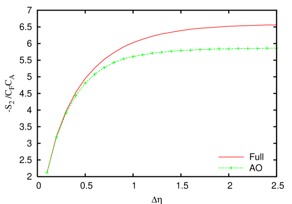
Figure 1: The coefficient of the leading order non-global contribution $-S_{2}/C_{F}C_{A}$ plotted as a function of the rapidity slice $\Delta\eta$ as given by both the full calculation and the angular-ordered approximation. The significant feature of saturation of the result for large slice-widths is apparent in both results.

We note once more that the $C_{F}^{2}$ independent-emission term of the squared matrix element is left intact since the angular-ordered and full results are identical for this piece, as one would expect. Making the modification described in Eq. (15) in each term of the $C_{F}C_{A}$ piece of the squared matrix element Eq. (7) and integrating over gluon directions we obtain the coefficient $S_{2}$ in the “angular ordered” (AO) approximation. We plot the numerical result in this approximation as a function of the gap size in Fig. 1 along with the full result. One can immediately observe that for small gap sizes the AO and full results are essentially identical. As one increases the gap size one notes a numerically significant difference between the two results although this is at best moderate. For instance for a slice of width $\Delta\eta=2.5$ one observes that the AO result is lower by $10.67\%$ than the full result. Additionally it is interesting to observe that the notable feature of saturation of $S_{2}$ for a large gap size is preserved by the AO approximation.

The reason the saturation property is preserved is because, as explained previously in detail, it arises from the region where the two gluons (respectively in and outside the gap region) are close in angle or equivalently from the region of integration $\eta_{1}\!-\!\eta_{2}\leq\Delta\eta$. Moreover, the bulk of the non-global contribution for any gap size arises from the region where the emission angles of the two soft gluons are of the same order. The contribution from configurations with the softest gluon at large angle relative to the next-softest gluon are small and vanish rapidly as we make the rapidity separation $\eta_{1}\!-\!\eta_{2}$ large.

In the AO approximation one requires the softest gluon $k_{2}$ to be emitted in a cone around the hard emitters $k_{1}$ and either the emitting quark leg $a$ or $b$, depending on whether one is looking at emission by dipole $ak_{1}$ or $bk_{1}$. The size of the cone is equal to the dipole opening angle. Thus the important region where $k_{1}$ and $k_{2}$ are collinear is perfectly described by the AO model. Only the region where $k_{2}$ is emitted at an angle larger than the cone opening angle would not be covered in the AO approximation and the contribution of such a region should be relatively small as we observe numerically. We mention in passing that these conclusions described explicitly for a rapidity slice are expected to hold for a general gap geometry and we explicitly checked the case of a square patch $\Delta\eta=\Delta\phi$ in rapidity and azimuth.

In the following section we shall examine the impact of the AO approximation at all orders to determine whether the encouraging fixed-order finding, that an AO model reproduces the characteristics and is numerically reasonably close to the full non-global result, can be extended to all orders, as one may now expect.

3 AO approximation at all orders

We now study the AO approximation by using the large $N_{c}$ evolution algorithm that was described in Ref. [13], suitably modifying it to take account of the angular ordering requirement. This should enable us to estimate how non-global logarithms will be simulated in an angular-ordered parton shower event generator. The algorithm works as follows. To compute the non-global contribution $S(\alpha_{s}L)$ where $L\equiv\ln(Q/Q_{\Omega})$ one considers the probability $P_{C}(L)$ of a configuration $C$ that does not resolve gluons above scale $L$, in other words those with energies below $Qe^{-L}$. The evolution of this configuration to another configuration $C^{\prime}$ with larger resolution scale $L^{\prime}$ or equivalently smaller energy scale, proceeds via soft emission of an extra gluon $k^{\prime}$ from the configuration $C$:

$$P_{C^{\prime}}(L^{\prime})=\bar{\alpha}_{s}(L^{\prime})\Delta_{C}(L,L^{\prime})P_{C}(L)F_{C}(\theta^{\prime},\phi^{\prime})\,,$$ (16)

where $\Delta_{C}(L,L^{\prime})$ represents the summation of only virtual gluons between the scales $L$ and $L^{\prime}$, $F_{C}(\theta^{\prime},\phi^{\prime})$ represents the angular pattern of emission of gluon $k^{\prime}$ from the system of dipoles in the configuration $C$ and $\bar{\alpha}_{s}\equiv\alpha_{s}/(2\pi)$. One has explicitly

$$F_{C}(\theta_{k},\phi_{k})=\sum_{\mathrm{dipoles-ij}}\frac{2C_{A}\left(1-\cos\theta_{ij}\right)}{\left(1-\cos\theta_{ik}\right)\left(1-\cos\theta_{jk}\right)}.$$ (17)

The same dipole angular pattern enters the pure virtual evolution probability (or form factor):

$$\ln\Delta_{C}(L,L^{\prime})=-\int_{L}^{L^{\prime}}\!\!dL^{\prime\prime}\!\int d\cos\theta\>d\phi\>\bar{\alpha}_{s}(L^{\prime\prime})\>F_{C}(\theta,\phi).$$ (18)

The probability that the interjet region $\Omega$ stays free of real emissions below a given scale $L$, is then given by summing over corresponding dipole configurations:

$$\Sigma(Q,Q_{\Omega})=\sum_{C\,|\,\Omega\,\mathrm{empty}}P_{C}(L)\,.$$ (19)

In order to obtain our angular-ordered results we need to modify the angular emission pattern $F_{C}$, as before for the fixed-order case, so we define

$$F_{C}(\theta_{k},\phi_{k})_{\mathrm{AO}}\equiv\sum_{\mathrm{dipoles-ij}}2C_{A}\left(\frac{\Theta\left(\cos\theta_{ik}-\cos\theta_{ij}\right)}{1-\cos\theta_{ik}}+\frac{\Theta\left(\cos\theta_{jk}-\cos\theta_{ij}\right)}{1-\cos\theta_{jk}}\right)\,.$$ (20)

Making the replacement $F_{C}(\theta_{k},\phi_{k})\to F_{C}(\theta_{k},\phi_{k})_{\mathrm{AO}}$ one modifies both real and virtual terms and obtains the result from our angular-ordered model at all orders:

$$\Sigma_{\mathrm{AO}}(Q,Q_{\Omega})=\sum_{C\,|\,\Omega\,\mathrm{empty}}P_{C,\mathrm{AO}}(L)\,.$$ (21)

Having obtained $\Sigma_{\mathrm{AO}}$ we can compare it with the full result without angular ordering. In Fig. 2 we plot the full and AO results for $\Sigma(t)$ as a function of $t$, for a slice of unit width $\Delta\eta=1$.

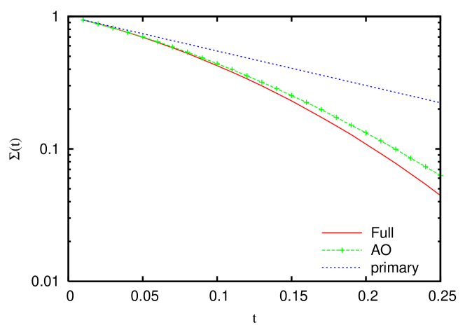
Figure 2: The integrated cross-section as a function of $t$ in the full calculation and the AO approximation. The primary result is also shown for reference.

One notes the relatively minor difference between the full and the AO results which indicates that the contribution to the full answer from regions where one can employ angular ordering, is the dominant contribution. For the sake of illustration we focus on the value $t=0.15$ which corresponds to a soft scale $Q_{\Omega}=1.0$ GeV for a hard scale $Q=100$ GeV. For the rapidity slice of unit width we note that the result for $\Sigma_{\mathrm{AO}}(t)$ is 9.68 $\%$ higher than the full result. At the same value of $t$, the difference between the full and the primary result, i.e. $\exp(-4\,C_{F}\,t)$, is around 75 $\%$, thus indicating that the AO approximation is much less significant than the role of the non-global component itself. Similar observations hold regardless of slice width.

One can also directly study the impact of the AO approximation on the pure non-global contribution $S(t)$. The primary contribution is unaffected by angular-ordering and can be divided out from the result for $\Sigma_{\mathrm{AO}}(t)$ to give us $S_{\mathrm{AO}}(t)$. We first take the example where $\Omega$ is a rapidity slice and consider different values for the slice width $\Delta\eta$. We illustrate in Fig. 3 three choices for the slice width $\Delta\eta=1.0,\,2.0,\,3.0$ with the full non-global contribution $S(t)$ and that in the AO model. We note that in both full and AO cases the feature of rough independence on the slice width $\Delta\eta$ is seen, as one can expect for sufficiently large slices. The AO curves are somewhat higher than the full ones indicating a somewhat smaller suppression than that yielded by the full calculation.

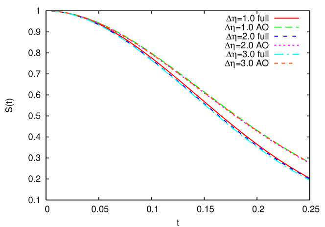
Figure 3: The resummed non-global contribution $S(t)$ as a function of $t$ in the full calculation and the AO approximation for different values of the slice width $\Delta\eta$. The upper set of curves correspond to the AO case and reflect that in that approximation a slightly smaller suppression is obtained than from the full calculation corresponding to the lower set of curves. The feature of rough independence on the slice width $\Delta\eta$ is visible in the full case and is preserved by the AO approximation.

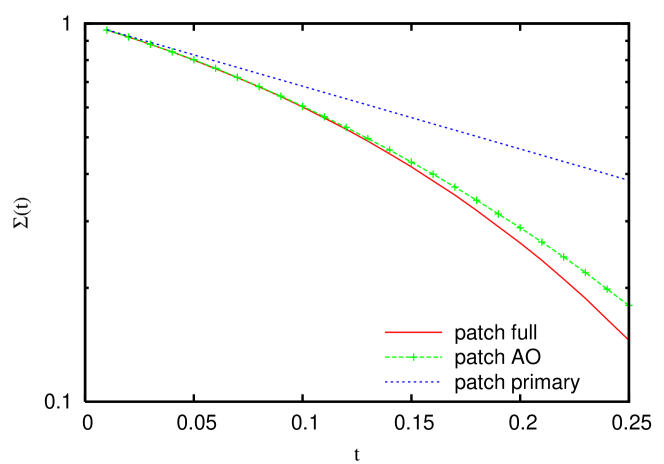
Figure 4: $\Sigma(t)$ vs $t$ for a square patch in rapidity and azimuth, $\Delta\eta=\Delta\phi=2.0$. Primary, full and angular-ordered (AO) curves are shown.

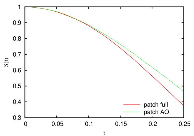
Figure 5: The non-global contribution $S(t)$ as a function of $t$ for a square patch in rapidity and azimuth, $\Delta\eta=\Delta\phi=2.0$.

Similar studies can be carried out for different geometries of $\Omega$. For a square patch in rapidity and azimuth with $\Delta\eta=\Delta\phi=2.0$, the full and angular-ordered results for $\Sigma(t)$ are shown in Fig. 4. The difference is seen to be small over a wide range of $t$. Once again focusing on the $t=0.15$ value, one notes that the AO approximation is only about three percent above the full result. At $t=0.2$ this difference rises to $9.75$ $\%$. Corresponding results for $S(t)$ for the same square patch, obtained by dividing by the primary result, are plotted in Fig. 5 and once again only a small to moderate effect is observed over the $t$ range shown.

We have thus observed that modifying the evolution code [13] used to compute the non-global logarithms, to impose angular ordering on them, only has a moderate effect on the quantity $S(t)$. This effect becomes even less significant for the quantity $\Sigma(t)=\Sigma_{P}(t)\,S(t)$ since the primary contribution $\Sigma_{P}(t)\equiv\exp[-4C_{F}A_{\Omega}t]$ is unchanged by imposing angular ordering, which we also explicitly checked with the code.

Having thus noted the small effect of the AO approximation within our model we would not expect much difference, in principle, between the results from an event generator based on angular-ordering in the soft limit (HERWIG) and the full non-global results. For PYTHIA, prior to the version 6.3 one may expect to see differences since angular ordering was imposed on top of ordering in the virtuality (invariant mass) of a splitting parton which leads to known problems with soft-gluon distributions, as discussed in [8]. In Ref. [18], where colour coherence effects were observed and studied at the Tevatron collider, it was in fact found that, unlike HERWIG, the PYTHIA event generator was not able to acceptably reproduce experimental observables sensitive to angular ordering. One may expect, however, that the new PYTHIA model [7, 8] (where, to our understanding, the improved shower, ordered in transverse momentum, better accounts for angular-ordering) results comparable to those from HERWIG may be obtained. In the next section our aim is to explore these issues and see if our expectations, outlined above, are indeed borne out.

4 Comparison with HERWIG and PYTHIA

In this section we shall focus on actual comparisons to results from HERWIG and PYTHIA. In order to meaningfully compare the results of a leading-log resummation with the parton level MC results, it is necessary to minimise the impact on the MC results of formally subleading and non-perturbative effects that are beyond full control and hence spurious.

In order to suppress subleading effects one needs to carry out the comparisons to the MC generators at extremely high values of $Q$, and hence we chose $10^{5}$ GeV. Thus effects that are formally of relative order $\alpha_{s}(Q)$ or higher can be expected to be negligible. A sign of this is the fact that at such large $Q$ values the MC results one obtains do not depend on $Q$ other than via the single logarithmic variable $t$ for a large range of $t$. It is clear that such high $Q$ values are beyond the reach of current or imminent collider experiments but since we are interested only in the dependence on $t$, the $Q$ value is fairly immaterial for our purposes. In fact one can take the conclusions we make for a particular $t$ value at $Q=10^{5}$ GeV and translate that into a value of $Q_{\Omega}$ for an experimentally realistic value of $Q$.

A clear source of uncertainty in this procedure is the different definitions of $\alpha_{{\textsc{s}}}$ in the resummation and the MC programs. In all resummed predictions we have used the LL expression for $t$:

$$t=\frac{1}{4\pi\beta_{0}}\ln\frac{1}{1-2\alpha_{{\textsc{s}}}(Q)\beta_{0}L}\,,\qquad\beta_{0}=\frac{11C_{A}-4T_{R}n_{f}}{12\pi}\>,$$ (22)

with $\beta_{0}$ corresponding to $n_{f}=6$ and $L$ given in Eq. (6). The coupling $\alpha_{{\textsc{s}}}(Q)$ is in the $\overline{\mathrm{MS}}$ scheme, and is obtained via a two-loop evolution with 6 active flavours from the input value $\alpha_{{\textsc{s}}}(M_{Z})=0.118$. This is to ensure that the resummed prediction is a function of $\alpha_{{\textsc{s}}}(Q)L$ only. HERWIG instead exploits a two-loop coupling in the physical CMW scheme [12] with $\alpha_{{\textsc{s}}}(M_{Z})=0.116$, while PYTHIA uses a one-loop coupling corresponding to $\alpha_{{\textsc{s}}}(M_{Z})=0.127$ [7]. The values of $t$ corresponding to different definitions of $\alpha_{{\textsc{s}}}$ (computed according to Eq. (6)) are found to be compatible within 10% in the considered $E_{t}$ range. This does not lead to appreciable modifications in the resummed curves plotted as a function of $E_{t}$ rather than $t$, in this section. Thus the comparisons we make below to the Monte Carlo results at a particular value of $E_{t}$ are not significantly affected by the issue of the somewhat different definitions employed in the resummation and the various Monte Carlo programs.

Another effect, not accounted for in the resummation, that is potentially significant, is the effect of quark masses (which would arise due to excitation of all flavours). These effects however can be safely neglected at the value of $Q$ we choose. In particular we also note that the presented MC curves are obtained by allowing the top quark to decay, but we have explicitly checked that we obtain almost identical results if we force the top quark to be stable.

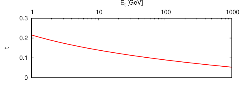
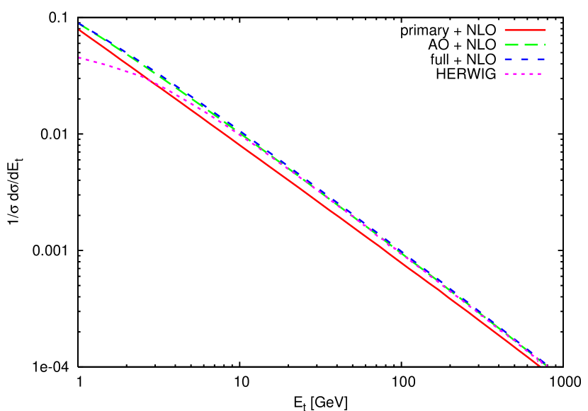
Figure 6: The distribution $\sigma^{-1}d\sigma/dE_{t}$ for a slice of $\Delta\eta=1$ and $Q=10^{5}~{}\mathrm{GeV}$ compared to parton shower results from HERWIG.

With the above observations in place, we start with the comparison to HERWIG which has a parton shower which is ordered (in the soft limit) in angle and thus one would expect results in line with those obtained via our AO model, introduced in previous sections. In Fig. 6 we show the results obtained from HERWIG compared to those from resummation for a rapidity interval of unit width. We note here that in order to obtain a sensible behaviour for the resummed predictions at large $E_{t}$, it was necessary to match the resummed results to exact fixed-order estimates. We carried out the so-called log-$R$ matching [1] to both leading and next-to–leading order (obtained from the numerical program EVENT2 [19]), but at the values of $E_{t}$ we have shown here, no significant difference was observed. The curves plotted in Fig. 6 are matched to NLO while the HERWIG results contain matrix-element corrections [20]. We observe that a very good agreement between HERWIG and the full and AO curves is seen over a significant range of $E_{t}$ values. We have also included the value of the variable $t$ as a function of $E_{t}$ to enable us to extrapolate our conclusions to lower centre-of-mass energies.

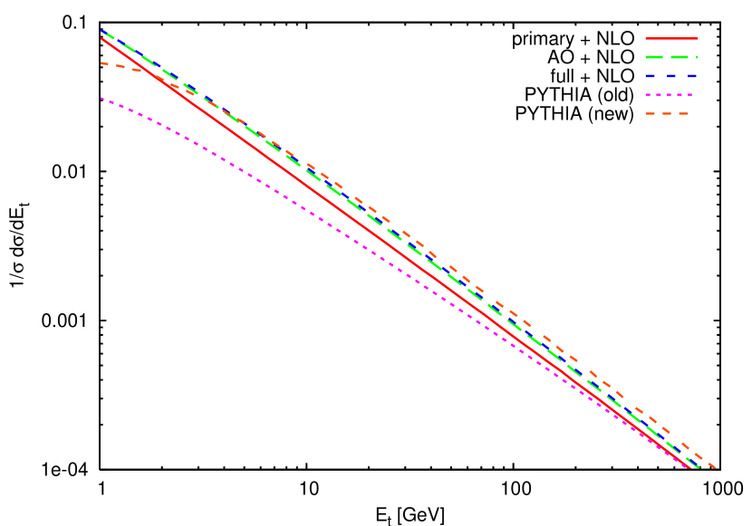
Figure 7: The distribution $\sigma^{-1}d\sigma/dE_{t}$ for a slice of $\Delta\eta=1$ and $Q=10^{5}~{}\mathrm{GeV}$ compared to parton shower results from PYTHIA.

The comparison to PYTHIA is shown in Fig. 7. We use version 6.3 and consider the old model, with showers ordered in virtuality and forced angular ordering, as well as the new model, where the emissions are ordered in transverse momentum. We note that the results obtained from PYTHIA with the new parton shower appear to be in reasonable agreement with the resummed curves including non-global logarithms, the situation being comparable to the quality of agreement one obtains with HERWIG. The same is not true for the old PYTHIA shower and a significant disagreement between the result there and the resummed curves is clearly visible.

In order to be more quantitative we focus on $E_{t}$ = 10 GeV which corresponds to a value of $t=0.15$. Here we note that the difference from the full resummed curve is respectively for HERWIG, PYTHIA (new) and PYTHIA (old) approximately $-10\%$, $+7.5\%$ and $50\%$. The difference between a resummed primary contribution and the full non-global result is, at the same value of $E_{t}$, $25\%$. We would then infer that if a variable of this type is chosen to tune for instance PYTHIA with the old shower (with ordering in the invariant mass) one includes potentially as much as $50\%$ of the leading-logarithmic perturbatively calculable contribution, to model-dependent parameters and incalculable effects such as hadronisation and the underlying event.

We have carried out our study for slices of different widths and obtain comparisons with HERWIG that are generally satisfactory. The same appears to be true of the new PYTHIA algorithm but here problems seem to crop up as one increases the slice rapidity. In Fig. 8 we present the comparison with both HERWIG and PYTHIA, but for a slice width $\Delta\eta=3.0$.

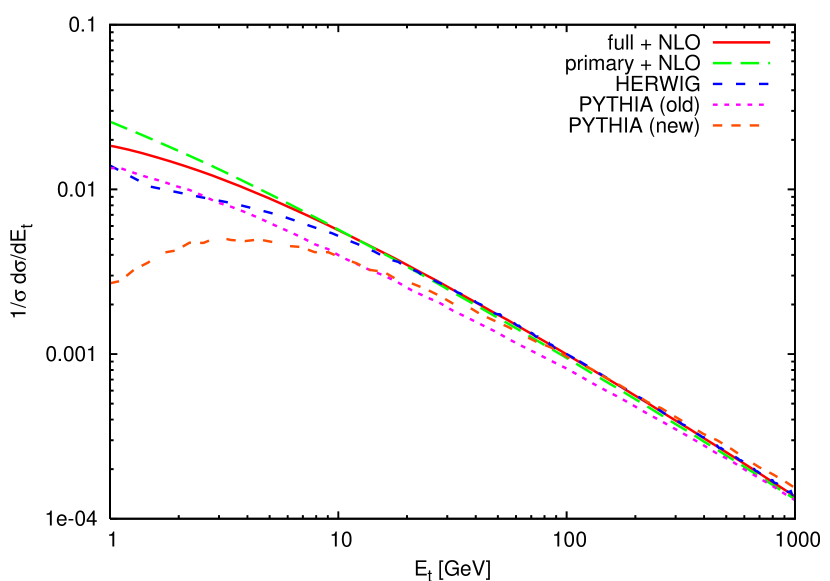
Figure 8: The distribution $\sigma^{-1}d\sigma/dE_{t}$ for a slice of $\Delta\eta=3.0$ and $Q=10^{5}~{}\mathrm{GeV}$.

We observe that for a larger slice the new PYTHIA shower at lower $E_{t}$ values yields a result that is significantly below all other predictions. The reason for this is not entirely obvious to us and we would welcome further insight into this observation. We have also carried out studies at other intermediate slice widths e.g. $\Delta\eta=2.0$ and it appears that the new PYTHIA curve starts to deviate from the resummed results at a value that is exponentially related to the slice width. This may signal that the new ordering variable in PYTHIA is perhaps not entirely satisfactory at large rapidities but as we mentioned a more detailed study is required to draw firm conclusions on this issue.

5 Conclusions

In this paper we have examined the role played by angular ordering in the calculation of the leading single-logarithmic terms that arise for non-global observables such as the away-from–jet energy flow. While it has been clear for some time [13, 14] that the fully correct single logarithmic resummed result cannot be obtained via use of angular ordering the question remained as to how much of the full result for such an observable may be captured by using the approximation of angular ordering. The reason this question arises in the first place is mainly because angular ordered parton showers are employed for example in Monte Carlo event generators such as HERWIG. Given the importance of these event generators as physics tools it is vital to understand the accuracy of the different ingredients thereof (such as the parton shower).

While the accuracy of the parton showers is generally claimed to be at least leading-logarithmic, this statement ought to apply only to those observables where the leading logarithms are double logarithms, i.e. both soft and collinear enhanced. However, to the best of our knowledge, there has been no discussion yet in the literature about non-global observables where the leading logarithms may be single logarithms instead of double logarithms and the accuracy of the parton showers in such instances. Since observables of the type we discuss here (energy or particle flows in limited regions of phase space) are often used in order to tune the parameters of the Monte Carlo algorithms (see e.g. [21] for examples and references), it is important to be at least aware of the fact the perturbative description yielded by the parton shower, may in these cases be significantly poorer than that obtained for instance for global observables. We have thus chosen one such observable and carried out a detailed study both of the role of angular ordering as well as the description provided by the most commonly used Monte Carlo event generators HERWIG and PYTHIA, compared to the full single-logarithmic result (in the large $N_{c}$ limit).

We find that in all the cases we studied, involving energy flow into rapidity slices or patches in rapidity and azimuth, angular ordering captures the bulk of the leading logarithmic contribution. This is a comforting finding but there remains the issue of precisely how angular ordering is embedded in the parton shower evolution for HERWIG and PYTHIA.

For HERWIG where the evolution variable in the soft limit is the emission angle one expects the agreement between parton shower and the leading-log resummed descriptions to be reasonable and we find that this is in fact the case.

In the case of the PYTHIA shower (prior to version 6.3) angular ordering is implemented by rejecting non-angular-ordered configurations in a shower ordered in virtuality. In this case it is clear that the description of soft gluons at large angles will be inadequate [8] and this feature emerges in our studies. From this we note that a discrepancy of around 50% could result while comparing PYTHIA to the correct leading-log result. This difference would be accounted for while tuning the parameters of PYTHIA to data and must be borne in mind, for instance while making statements on the tuning of the hadronisation corrections and the underlying event into the PYTHIA model. This is because a tuning to energy flows would mean that significant leading-logarithmic (perturbatively calculable) physics is mixed with model-dependent non-perturbative effects which does not allow for the best possible description of either. Moreover, the non-global effects are not universal and thus incorporating them into the generic shower and non-perturbative parameters will lead to a potentially spurious description of other (global) observables.

The new PYTHIA shower, ordered in transverse momentum and with a more accurate treatment of angular ordering, does however give a good description of the leading logarithmic perturbative physics, comparable to that obtained from HERWIG. However, for large rapidity slices we find that problems emerge in the description provided by PYTHIA even with the new shower. The origin of these problems is not entirely clear to us and we would welcome further insight here. Hence, we strongly emphasise the need to compare the shower results from HERWIG and PYTHIA while carrying out studies of observables that involve energy flow into limited regions of phase space. Where this difference is seen to be large, care must be taken about inferences drawn from these studies about the role of non-perturbative effects, such as hadronisation and the underlying event. We believe that further studies and discussions of the issues we have raised here are important in the context of improving, or at the very least understanding, the accuracy of some aspects of Monte Carlo based physics studies.

Acknowledgements.

We would like to thank Giuseppe Marchesini, Gavin Salam and Mike Seymour for useful discussions. One of us (MD) gratefully acknowledges the hospitality of the LPTHE, Paris Jussieu, for their generous hospitality while this work was in completion.

References

-
[1]
S. Catani, L. Trentadue, G. Turnock and B. R. Webber,
Resummation of large logarithms in event shape distributions,
Nucl. Phys. B 407 (1993) 3;
S. Catani, G. Turnock, B. R. Webber and L. Trentadue, Thrust distribution in annihilation, Phys. Lett. B 263 (1991) 491. -
[2]
A. Banfi, G. P. Salam and G. Zanderighi,
Principles of general final-state resummation and automated
implementation,
J. High Energy Phys. 03 (2005) 073
hep-ph/0407286;
Generalized resummation of QCD final-state observables, Phys. Lett. B 584 (2004) 298 hep-ph/0304148. - [3] A. Banfi, G. P. Salam and G. Zanderighi, Semi-numerical resummation of event shapes, J. High Energy Phys. 01 (2002) 018 hep-ph/0112156.
- [4] G. Corcella et al., HERWIG 6: An event generator for hadron emission reactions with interfering gluons (including supersymmetric processes), J. High Energy Phys. 01 (2001) 010 hep-ph/0011363.
- [5] S. Gieseke, A. Ribon, M. H. Seymour, P. Stephens and B. Webber, Herwig++ 1.0: an event generator for annihilation, J. High Energy Phys. 02 (2004) 005 hep-ph/0311208.
- [6] T. Sjostrand, P. Eden, C. Friberg, L. Lonnblad, G. Miu, S. Mrenna and E. Norrbin, High-energy-physics event generation with PYTHIA 6.1, Comput. Phys. Commun. 135 (2001) 238 hep-ph/0010017.
- [7] T. Sjostrand, S. Mrenna and P. Skands, PYTHIA 6.4 physics and manual, J. High Energy Phys. 05 (2006) 026 hep-ph/0603175.
- [8] T. Sjostrand and P. Z. Skands, Transverse-momentum-ordered showers and interleaved multiple interactions, Eur. Phys. J. C 39 (2005) 129 hep-ph/0408302.
-
[9]
Y. L. Dokshitzer, D. Diakonov and S. I. Troyan,
Hard processes in Quantum Chromodynamics,
Phys. Rept. 58 (1980) 269;
A. Bassetto, M. Ciafaloni and G. Marchesini, Jet structure and infrared sensitive quantities in perturbative QCD, Phys. Rept. 100 (1983) 201. - [10] H. U. Bengtsson and G. Ingelman, The Lund Monte Carlo for high P(T) physics, Comput. Phys. Commun. 34 (1985) 251.
- [11] G. Marchesini and B. R. Webber, Simulation of QCD jets including soft gluon interference, Nucl. Phys. B 238 (1984) 1.
- [12] S. Catani, G. Marchesini and B. R. Webber, QCD coherent branching and semiinclusive processes at large x, Nucl. Phys. B 349 (1991) 635.
- [13] M. Dasgupta and G. P. Salam, Resummation of non-global QCD observables, Phys. Lett. B 512 (2001) 323 hep-ph/0104277.
- [14] M. Dasgupta and G. P. Salam, Accounting for coherence in interjet E(t) flow: a case study, J. High Energy Phys. 03 (2002) 017 hep-ph/0203009.
- [15] A. Banfi, G. Marchesini and G. Smye, Away-from-jet energy flow, J. High Energy Phys. 0208 (2002) 006 hep-ph/0206076.
- [16] G. Marchesini and B. R. Webber, Monte Carlo simulation of general hard processes with coherent QCD radiation, Nucl. Phys. B 310 (1988) 461.
- [17] L. Lonnblad, Ariadne version 4: a program for simulation of QCD cascades implementing the Color Dipole Model, Comput. Phys. Commun. 71 (1992) 15.
- [18] F. Abe et al. [CDF Collaboration], Evidence for color coherence in collisions at TeV, Phys. Rev. D 50 (1994) 5562.
- [19] S. Catani and M. H. Seymour, A general algorithm for calculating jet cross sections in NLO QCD, Nucl. Phys. B 485 (1997) 291, Erratum ibid. B 510 (1998) 503 hep-ph/9605323; The dipole formalism for the calculation of QCD jet cross sections at next-to-leading order, Phys. Lett. B 378 (1996) 287 hep-ph/9602277.
- [20] M. H. Seymour, Photon radiation in final state parton showering, Z. Physik C 56 (1992) 161.
- [21] A. A. Affolder et al. [CDF Collaboration], Charged jet evolution and the underlying event in collisions at 1.8 TeV, Phys. Rev. D 65 (2002) 092002.