A Positive-Weight Next-to-Leading-Order Monte Carlo for Annihilation to Hadrons
Abstract:
We apply the positive-weight Monte Carlo method of Nason for simulating QCD processes accurate to Next-To-Leading Order to the case of annihilation to hadrons. The method entails the generation of the hardest gluon emission first and then subsequently adding a ‘truncated’ shower before the emission. We have interfaced our result to the Herwig++ shower Monte Carlo program and obtained better results than those obtained with Herwig++ at leading order with a matrix element correction.
KA–TP–10–2006
1 Introduction
Matching next-to-leading order (NLO) calculations to shower Monte Carlo (SMC) models is highly non-trivial. One method (MC@NLO) has been proposed in [1] and has been successfully applied to several processes [2, 3] in connection with the FORTRAN HERWIG parton shower. One drawback of the method is the generation of negative weighted events which are unphysical.
An alternative method proposed in [4] overcomes the negative weight problem. It has successfully been applied to Z pair hadroproduction [5] and involves the generation of the hardest radiation independently of the SMC model used to generate the parton shower. To preserve the soft radiation distribution, the addition of a ‘truncated shower’ of soft coherent radiation before the hardest emission is necessary. In this report, we will be implementing this method for electron-positron annihilation to hadrons at a centre-of-mass energy of GeV. The SMC we will be employing is Herwig++ [6] which will perform the rest of the showering, hadronization and decays.
In Section 2, we discuss the generation of the hardest emission according to the matrix element via a modified Sudakov form factor. In Section 3, we go on to describe the generation of a simplified form of the ‘truncated’ shower. We determine the probability for the emission of at most one gluon before the hardest emission and re-shuffle the momenta of the outgoing particles accordingly. This is a reasonable first approximation since the probability of emitting an extra gluon is small.
2 Hardest emission generation
2.1 Hardest emission cross section
The order- differential cross section for the process , neglecting the quark masses, can be written as
| (1) |
where is the Born cross section, , and are the energy fractions of the quark and antiquark and is the energy fraction of the gluon. has collinear singularities when the quark or antiquark is aligned with the gluon. When combined with the virtual corrections, these singularities can be integrated to give the well known total cross section to order-,
| (2) |
From [4], we can write the cross section for the hardest gluon emission event as
| (3) |
where is the Born cross section and is the Born variable, which in this case is the angle between the beam axis and the axis. represents the radiation variables ( and for our specific case), and are the Born and real emission phase spaces respectively.
is the modified Sudakov form factor for the hardest emission with transverse momentum , as indicated by the Heaviside function in the exponent of (4),
| (4) |
Furthermore,
| (5) |
is the sum of the Born, , virtual, and real, terms, (with some counter-terms, ). It overcomes the problem of negative weights since in the region where is negative, the NLO negative terms must have overcome the Born term and hence perturbation theory must have failed. Now explicitly for annihilation,
| (6) |
where and are the energy fractions of the quark and antiquark and we define
| (7) |
and as the square of the center-of-mass energy. is the transverse momentum of the hardest emitted gluon relative to the splitting axis, as illustrated in Figure 1 below.

2.2 Generation of radiation variables, and
From (1) and (3), it can be deduced that the radiation variables are to be generated according to the probability distribution
| (8) |
where in the particular case of annihilation, and are given in (6) and (1) respectively. However for ease of integration, we will use a function
| (9) |
in place of . As we shall see later, the true distribution is recovered using the veto technique. The variables and are then generated according to
| (10) |
This is outlined in the following steps:
-
i)
Set .
-
ii)
For a random number, between and , solve the equation below for
(11) -
iii)
Generate the variables and according to the distribution
(12) -
iv)
Accept the generated value of with probability . If the event is rejected set and go to step ii).
Now for annihilation,
| (13) |
In the region where , let’s define the dimensionless variable, as
| (14) |
There are 2 solutions for for each value of and , i.e and .
| (15) |
Exchanging the variable for in (13) we find
where
| (17) |
Note that the argument of is the scale with
MeV.
Equation (2.2) applies to the region of phase space where . For the region ,
and are exchanged in the equation.
The integration can be performed to yield
| (18) | |||||
For , the region of phase space where and the two solutions for for given values of and are illustrated in Figure 2 below.

The two solutions lie on either side of the dashed line and are equal when which lies on the dotted line. At , the branches meet along the line and there is only one solution for in the region (the lower branch). So for , only one solution exists. In addition there are no solutions for . This is illustrated in Figure 3.
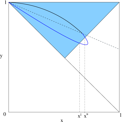
Also note that for , there is only one solution for .
In the region where there are two solutions, the integral in (18) is performed along both branches independently and summed. For the upper branch, runs from to while for the lower branch, runs from to where if we define
| (19) |
we can write and as;
| (20) |
In the region where there is only one solution for , runs from to .
The integration can then be performed numerically. Having performed the
integration, values for and hence are then generated according to steps 1 and 2 in
Section 2.2. In step 3 of Section 2.2, the variables and are to be
distributed according to . This is the subject of the next section.
2.3 Distributing and according to
To generate and values with a distribution proportional to , we can use the -function to eliminate the variable by computing
| (21) |
where is such that . Note that is the same for both solutions. We then generate values with a probability distribution proportional to with hit-and-miss techniques as described below. All events generated have uniform weights.
-
i)
Randomly sample , times (we used ) in the range for the selected value of .
-
ii)
For each value of , evaluate if there are two solutions for the selected and if there is only one solution. Also, if and (see Figure 2), there is only one solution so evaluate .
-
iii)
Find the maximum value of for the selected value of from the set of points that have been sampled.
-
iv)
Next, select a value for in the allowed range and evaluate .
-
v)
If (where is a random number between and ), accept the event, otherwise go to iv) and generate a new value for .
-
vi)
If for the chosen value of , there are two solutions for , select a value for in the ratio .
-
vii)
Compare with the true matrix element, . If the event fails this veto, set and regenerate a new value as discussed in Section 2.2.
NB: For the region , exchange and in the above discussion. In this way, the smooth phase space distribution in Figure 4 below was obtained for the hardest emission events. The plot show 2,500 of these events.

3 Adding the truncated shower
As mentioned in Section 1, a ‘truncated shower’ would need to be added before the hardest emission to simulate the soft radiation distribution. Due to angular ordering, the ‘truncated’ radiation is emitted at a wider angle than the angle of the hardest emission as well as a lower . This means the ‘truncated’ radiation does not appreciably degrade the energy entering the hardest emission and justifies our decision to generate the hardest emission first.
Below is an outline of how the ‘truncated shower’ was generated. We will consider the case in which at most one extra gluon is emitted by the quark or antiquark before the hardest emission. The outline closely follows the Herwig++ parton shower evolution method described in [6, 7] where the evolution variables , the momentum fractions, and , the evolution scale, determine the kinematics of the shower.
-
i)
Having generated the of the hardest emission and the energy fractions and , calculate the momentum fraction and of the partons involved in the hardest emission. We will assume henceforth that and that is the energy fraction of the quark, i.e. the quark is involved in the hardest emission. Then
(22) where as defined above and are the momentum fractions of the quark and gluon respectively.
-
ii)
Next generate the momentum fraction of the ‘truncated’ radiation according to the splitting function within the range
(23) where is the initial evolution scale, i.e. GeV, =max(), is the mass of the quark and is a cutoff introduced to regularize soft gluon singularities in the splitting functions. In this report, a value of GeV (and hence GeV) was used. is the momentum fraction of the quark after emitting the ‘truncated’ gluon with momentum fraction .
-
iii)
Having generated a value for , determine the scale of the hardest emission from
(24) where .
-
iv)
Starting from an initial scale , the probability of there being an emission next at the scale is given by
(25) where
(26) is the lower cutoff of the parton shower which was set to GeV in this report, is the running coupling constant evaluated at , is the splitting function and is the transverse momentum of the hardest emission. The Heaviside function ensures that the transverse momentum, of the truncated emission is real and is less than . To evaluate the integral in (26), we overestimate the integrands and apply vetoes with weights as described in [6]. With a random number between and , we then solve the equation
(27) for . If , the event has a ‘truncated’ emission. If , there is no ‘truncated’ emission and the event is showered from the scale of the hardest emission.
-
v)
If there is a ‘truncated’ emission, the next step is to determine the transverse momentum of the emission. This is given by [6]
(28) If or go to ii).
-
vi)
We now have values for , the momentum fraction of the quark after the first emission, , the transverse momentum of the first emission, , the momentum fraction of the hardest emission and , the transverse momentum of the hardest emission. This is illustrated in Figure 5. We can then reconstruct the momenta of the partons as described in [6]. The orientation of the quark, antiquark and hardest emission with respect to the beam axis is determined as explained there for the hard matrix element correction.

Figure 5: Adding the ‘truncated’ emission. ( GeV)
In principle this procedure could be iterated to generate a multi-gluon truncated shower. However, for the present, we consider only the effect of at most one extra gluon emission. As discussed in [4], the initial showering scale of the hardest gluon is set equal to the showering scale of the quark or antiquark closest in angle to it. This gives the right amount of soft radiation colour connected to the gluon line.
4 Results and data comparisons
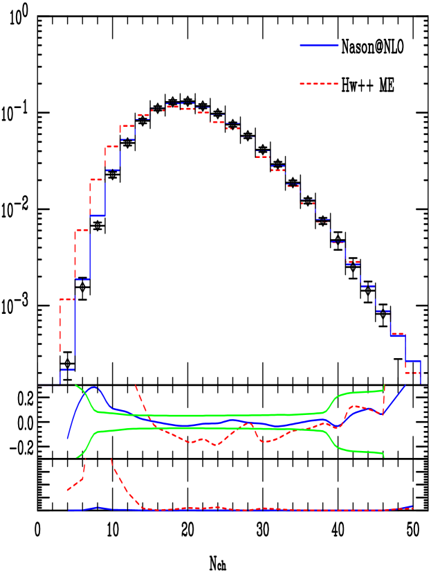
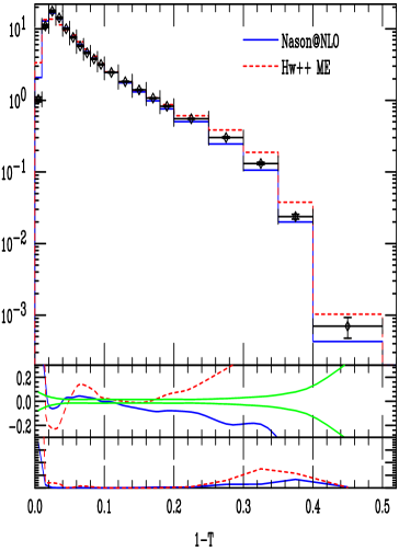
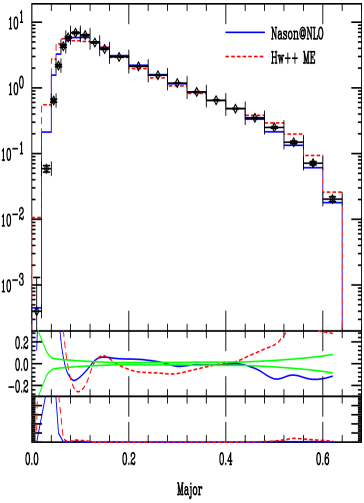
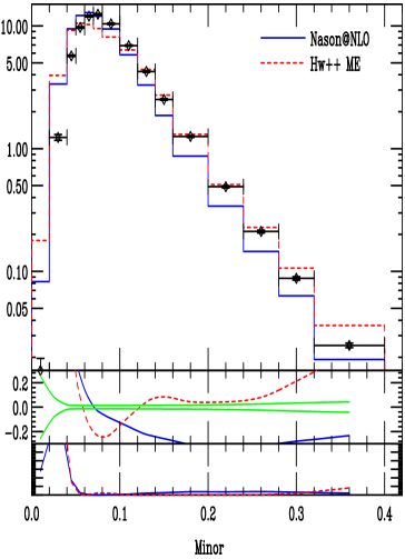
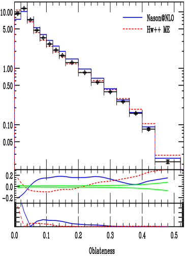
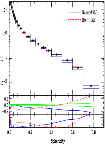
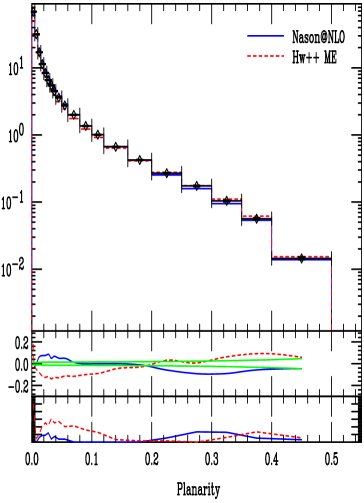
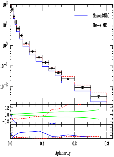
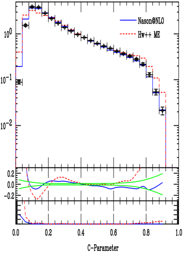
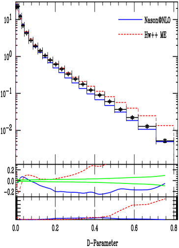
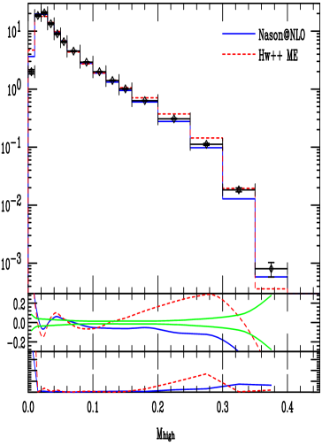
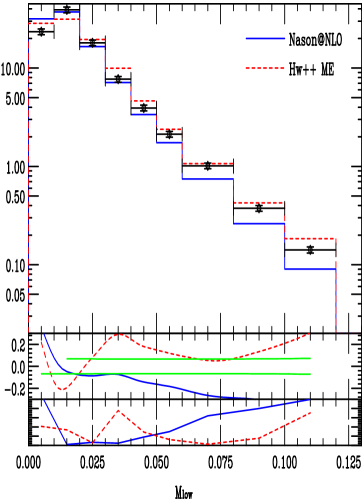
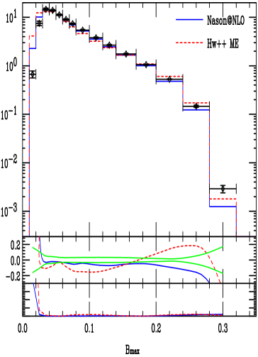
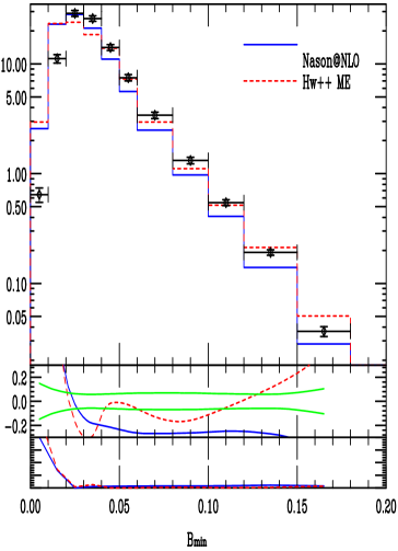
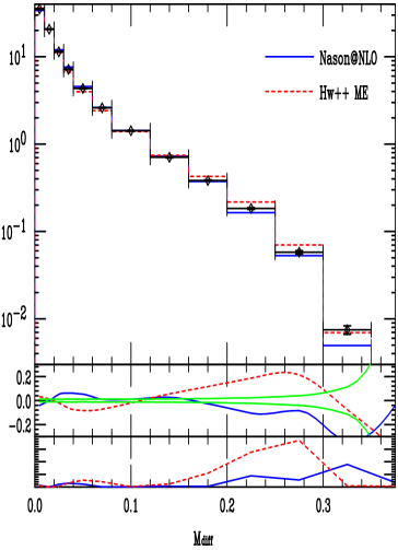
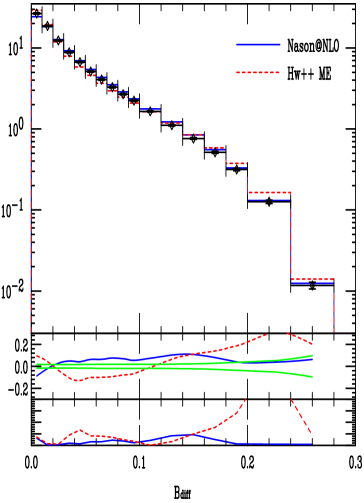
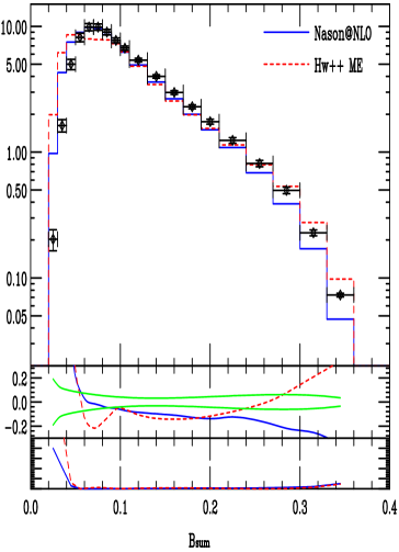
One million events were generated as described above and then interfaced with the SMC, Herwig++. of the events acquired an extra ‘truncated’ gluon. A veto was imposed on the subsequent shower starting from the hardest emission to the hadronization scale which was tuned to GeV. Table LABEL:tab:mult and Figure 6 show respectively the average multiplicities of a wide range of hadron species and the charged particle multiplicity distribution. The subsequent figures are plots of comparisons with event shape distributions from the DELPHI experiment at LEP [8].
The upper panel below the main histograms shows the ratio (where and stand for Monte Carlo result and data value respectively) compared with the relative experimental error (green). The lower panel shows the relative contribution to the of each observable. As in [6], the contributions allow for a uncertainty in the predictions if the data are more accurate than this. Finally, in Table 2 we show a list of values for all observables that were studied during the analysis. The results were generated using Herwig++ [9] which includes some improvements in the simulation of the shower and hadronization as described in [9] leading to some changes in the for specific observables relative to [6], although in most cases the changes are small.
5 Conclusions
We have successfully implemented the Nason method of generating the hardest emission first and subsequently adding a truncated shower for annihilation into hadrons.
We have tested the method against data from colliders and for almost all examined observables, the simulation of the data is improved with respect to Herwig++. In particular the Nason method seems to fit the data better in the soft regions of phase space. The poorer fits obtained for variables such as the thrust minor which vanish in the three-jet limit (and in general for planar events) may be attributable to the lack of multiple emission in the truncated shower.
The fits are summarized in the values shown in Table 2. In Table 2 we also present the values for the observables obtained without the implementation of the ‘truncated’ shower. We see there is a general improvement in the fits associated with the addition of the ‘truncated’ emissions.
Future work in this area will extend this method to processes with initial state radiation in hadron-hadron collisions aiming at simulating Tevatron and LHC events.
Acknowledgements
We are most grateful to all the other members of the Herwig++ collaboration for developing the program that underlies the present work. This work was supported in part by the UK Particle Physics and Astronomy Research Council.
| Particle | Experiment | Measured | Herwig++ ME | Nason@NLO |
|---|---|---|---|---|
| All Charged | M,A,D,L,O | 20.924 0.117 | ||
| A,O | 21.27 0.6 | |||
| A,D,L,O | 9.59 0.33 | |||
| A,D | 1.295 0.125 | |||
| A,O | 17.04 0.25 | |||
| O | 2.4 0.43 | |||
| A,L,O | 0.956 0.049 | |||
| A,L,O | 1.083 0.088 | |||
| A,L,O | 0.152 0.03 | |||
| S,A,D,L,O | 2.027 0.025 | |||
| A,D,O | 0.761 0.032 | |||
| D,O | 0.106 0.06 | |||
| A,D,O | 2.319 0.079 | |||
| A,D,O | 0.731 0.058 | |||
| A,D,O | 0.097 0.007 | |||
| A,D,O | 0.991 0.054 | |||
| D,O | 0.088 0.034 | |||
| O | 0.083 0.011 | |||
| A,D,L,O | 0.373 0.008 | |||
| A,D,O | 0.074 0.009 | |||
| O | 0.099 0.015 | |||
| A,D,O | 0.0471 0.0046 | |||
| A,D,O | 0.0262 0.001 | |||
| A,D,O | 0.0058 0.001 | |||
| A,D,O | 0.00125 0.00024 | |||
| D,L,O | 0.168 0.021 | |||
| D | 0.02 0.008 | |||
| A,D,O | 0.184 0.018 | |||
| A,D,O | 0.182 0.009 | |||
| A,D,O | 0.473 0.026 | |||
| A,O | 0.129 0.013 | |||
| O | 0.096 0.046 | |||
| A,D,L,O | 0.00544 0.00029 | |||
| D,O | 0.077 0.016 | |||
| D,L,O | 0.00229 0.00041 |
| Observable | Herwig++ ME | Nason@NLO | Nason@NLO |
|---|---|---|---|
| with truncated shower | w/o truncated shower | ||
| 36.52 | 9.03 | 9.81 | |
| Thrust Major | 267.22 | 36.44 | 37.65 |
| Thrust Minor | 190.25 | 86.30 | 90.59 |
| Oblateness | 7.58 | 6.86 | 6.28 |
| Sphericity | 9.61 | 7.55 | 9.01 |
| Aplanarity | 8.70 | 22.96 | 25.33 |
| Planarity | 2.14 | 1.19 | 1.45 |
| Parameter | 96.69 | 10.50 | 11.14 |
| Parameter | 84.86 | 8.89 | 10.88 |
| 14.70 | 5.31 | 6.61 | |
| 7.82 | 12.90 | 13.44 | |
| 5.11 | 1.89 | 2.09 | |
| 39.50 | 11.42 | 12.17 | |
| 45.96 | 35.2 | 36.16 | |
| 91.03 | 28.83 | 30.58 | |
| 8.94 | 1.40 | 1.14 | |
| 43.33 | 1.58 | 10.08 | |
| 56.47 | 16.96 | 18.49 |
References
- [1] S. Frixione and B. R. Webber, “Matching NLO QCD computations and parton shower simulations,” JHEP 06 (2002) 029, hep-ph/0204244.
- [2] S. Frixione, P. Nason, and B. R. Webber, “Matching NLO QCD and parton showers in heavy flavour production,” JHEP 08 (2003) 007, hep-ph/0305252.
- [3] S. Frixione and B. R. Webber, “The MC@NLO 3.3 event generator,” hep-ph/0612272.
- [4] P. Nason, “A new method for combining NLO QCD with shower Monte Carlo algorithms,” JHEP 11 (2004) 040, hep-ph/0409146.
- [5] P. Nason and G. Ridolfi, “A positive-weight next-to-leading-order Monte Carlo for Z pair hadroproduction,” JHEP 08 (2006) 077, hep-ph/0606275.
- [6] S. Gieseke, A. Ribon, M. H. Seymour, P. Stephens, and B. Webber, “Herwig++ 1.0: An event generator for annihilation,” JHEP 02 (2004) 005, hep-ph/0311208.
- [7] S. Gieseke, P. Stephens, and B. Webber, “New formalism for QCD parton showers,” JHEP 12 (2003) 045, hep-ph/0310083.
- [8] DELPHI Collaboration, P. Abreu et al., “Tuning and test of fragmentation models based on identified particles and precision event shape data,” Z. Phys. C73 (1996) 11–60.
- [9] S. Gieseke et al., “Herwig++ 2.0 release note,” hep-ph/0609306.
- [10] B. R. Webber, “Fragmentation and hadronization,” hep-ph/9912292.
- [11] OPAL Collaboration, P. D. Acton et al., “A study of charged particle multiplicities in hadronic decays of the Z0,” Z. Phys. C53 (1992) 539–554.