Antenna subtraction with hadronic initial states

Abstract:

The antenna subtraction method for the computation of higher order corrections to jet observables and exclusive cross sections at collider experiments is extended to include hadronic initial states. In addition to the already known antenna subtraction with both radiators in the final state (final-final antennae), we introduce antenna subtractions with one or two radiators in the initial state (initial-final or initial-initial antennae). For those, we derive the phase space factorization and discuss the allowed phase space mappings at NLO and NNLO. We present integrated forms for all antenna functions relevant to NLO calculations, and describe the construction of the full antenna subtraction terms at NLO on two examples. The extension of the formalism to NNLO is outlined.

1 Introduction

The calculation of perturbative higher order corrections to exclusive observables (especially jet production cross sections, but also transverse momentum or rapidity distributions) requires a systematic procedure to extract infrared singularities from real radiation contributions. These singularities arise if one or more final state particles become soft or collinear. For the task of next-to-leading order (NLO) calculations [1] several systematic and process-independent procedures are available. Except for the phase space slicing technique [2], all these methods [3, 4, 5, 6, 7] work by introducing additional terms, that are subtracted from the real radiation matrix element at each phase space point. These subtraction terms approximate the matrix element in all singular limits, and are sufficiently simple to be integrated over part of the phase space analytically. After this integration, infrared divergences of the subtraction terms are made explicit, and the integrated subtraction terms can be added to the virtual corrections, thus yielding an infrared finite result. One of these subtraction methods is antenna subtraction [5, 6], which constructs the subtraction terms from so-called antenna functions. These antenna functions describe all unresolved partonic radiation (soft and collinear) between a hard pair of radiator partons.

Extensions to next-to-next-to-leading order (NNLO) are discussed in the literature for phase space slicing [8], and for several subtraction methods [9, 10, 11, 12, 13, 14]. A completely independent approach, avoiding the need for analytical integration is the sector decomposition method, which has been derived for virtual [15] and real radiation [16] corrections to NNLO, and applied to several observables already [17]. Among the subtraction methods, only the NNLO formulation of the antenna subtraction method [14] is worked out to a sufficient extent to be readily implemented in the calculation of NNLO corrections to a physical process. Using this method, the calculation of $e^{+}e^{-}\to 3$ jets at NNLO accuracy is currently under way [18]. However, up to now, the antenna subtraction (both at NLO and NNLO) method was developed only to handle unresolved singular radiation off final state partons. An extension to radiation off initial state partons was missing so far for this method, while all other NLO subtraction methods could handle radiation off initial and final state particles.

It is the purpose of this paper to extend the antenna subtraction method to include radiation off initial state partons, such that it can be used in the calculation of higher order corrections to processes at lepton-hadron or hadron-hadron colliders. In Section 2, we recall the structure of antenna subtraction terms and describe their systematic derivation. Antenna subtraction for radiation off final state partons was formulated already in [6, 5, 14] and is briefly summarized in Section 3. In Sections 4 and 5, we present a detailed derivation of antenna subtraction for situations with one or two radiator partons in the initial state. In these sections, we provide all necessary ingredients for an implementation at NLO, and discuss the extension to NNLO. To illustrate the application method, we describe two NLO examples in Section 6. Finally, Section 7 contains conclusions and an outlook.

2 Antenna subtraction

To obtain the perturbative corrections to a jet observable at a given order, all partonic multiplicity channels contributing to that order have to be summed. In general, each partonic channel contains both ultraviolet and infrared (soft and collinear) singularities. The ultraviolet poles are removed by renormalisation in each channel. Collinear poles originating from radiation off incoming partons are an inherent feature of the incoming partons, and are cancelled by redefinition (mass factorization) of the parton distributions. The remaining soft and collinear poles cancel among each other only when all partonic channels are summed over.

While infrared singularities from purely virtual corrections are obtained immediately after integration over the loop momenta, their extraction is more involved for real emission (or mixed real-virtual) contributions. Here, the infrared singularities only become explicit after integrating the real radiation matrix elements over the phase space appropriate to the jet observable under consideration. In general, this integration involves the (often iterative) definition of the jet observable, such that an analytic integration is not feasible (and also not appropriate). Instead, one would like to have a flexible method that can be easily adapted to different jet observables or jet definitions. Therefore, the infrared singularities of the real radiation contributions should be extracted using infrared subtraction terms. The crucial points that all subtraction terms must satisfy are that (a) they approximate the full real radiation matrix elements in all singular limits and (b) are still sufficiently simple to be integrated analytically over a section of phase space that encompasses all regions corresponding to singular configurations.

For NLO calculations, several different methods are available to derive subtraction terms in a process-independent way [3, 4, 6, 5, 7]. One of these methods is the so-called antenna subtraction [6, 5].

In this method, antenna functions describe the colour-ordered radiation of unresolved partons between a pair of hard (radiator) partons. All antenna functions at NLO and NNLO can be derived systematically from physical matrix elements, as shown in [14, 19]. They can be integrated over the factorized antenna phase space [9] using loop integral reduction techniques extended to phase space integrals [21], and then combined with virtual corrections to partonic processes with lower multiplicity.

Up to now, antenna subtraction has been formulated at NLO [6, 5] and NNLO [14] only for processes with a colourless initial state. In this case, both radiator partons are in the final state, we call this situation a final-final antenna. For collider observables involving hadronic initial states, there can be either one or both partons in the initial state. Unresolved radiation off these initial state partons can also be subtracted using antenna functions, with one or two radiators in the initial state. We call these initial-final and initial-initial antennae. The radiated parton is always in the final state. Figures 1–3 illustrate how a single unresolved parton can be emitted between radiators in the final or initial state, and show how all these situations are factorized into antenna functions. Each antenna contains both collinear limits of the unresolved parton with either radiator as well as the soft limit.

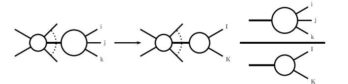
Figure 1: Antenna factorization for the final-final situation.

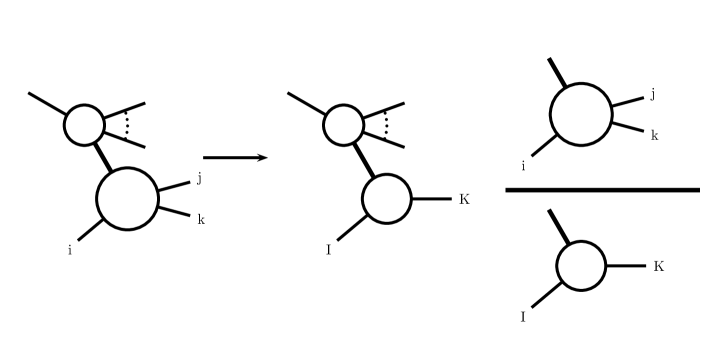
Figure 2: Antenna factorization for the initial-final situation.

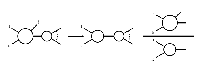
Figure 3: Antenna factorization for the initial-initial situation.

In each situation, the subtraction term is constructed from products of antenna functions with reduced matrix elements (with fewer final state partons than the original matrix element), and integrated over a phase space which is factorized into an antenna phase space (involving all unresolved partons and the two radiators) multiplied with a reduced phase space (where the momenta of radiators and unresolved radiation are replaced by two redefined momenta). These redefined momenta can be in the initial state, if the corresponding radiator momenta were in the initial state. The full subtraction term is obtained by summing over all antennae required for the problem under consideration. In the most general case (two partons in the initial state, and two or more hard partons in the final state), this sum includes final-final, initial-final and initial-initial antennae.

To specify the notation, we consider the hadronic cross section

$$\hbox{d}\sigma=\sum_{a,b}\int\frac{\hbox{d}\xi_{1}}{\xi_{1}}\frac{\hbox{d}\xi_{2}}{\xi_{2}}\,f_{a/1}(\xi_{1})\,f_{b/2}(\xi_{2})\,\hbox{d}\hat{\sigma}(\xi_{1}H_{1},\xi_{2}H_{2})\;,$$ (1)

where $\xi_{1}$ and $\xi_{2}$ are the momentum fractions of the partons of species $a$ and $b$ in both incoming hadrons, with $f$ being the corresponding parton distribution functions and $H_{1,2}$ denoting the incoming hadron momenta. The cases of only one or no incoming hadrons are obtained trivially by replacing the relevant $f(\xi)$ by $\delta(1-\xi)$. The dependence of the parton-level cross section $\hbox{d}\hat{\sigma}$ on the parton species $a,b$ is obvious, and not stated explicitly for ease of notation. It should be noted that the parton level cross section $\hbox{d}\hat{\sigma}$ is normalized to the hadron-hadron flux factor, which is transformed into the parton-parton flux factor by dividing out $\xi_{1}$ and $\xi_{2}$ in the above.

We define the partonic tree-level $n$-parton contribution to the $m$-jet cross section (for tree-level cross sections $n=m$; we leave $n\neq m$ for later reference) in $d$ dimensions by,

$${\rm d}\hat{\sigma}(p_{1},p_{2}) = {\cal N}\,\sum_{{n}}{\rm d}\Phi_{n}(k_{1},\ldots,k_{n};p_{1},p_{2})$$ (2)

$$\times\frac{1}{S_{{n}}}\,|{\cal M}_{n}(k_{1},\ldots,k_{n};p_{1},p_{2})|^{2}\;J_{m}^{(n)}(k_{1},\ldots,k_{n}).$$

The definition of the observable $J_{m}^{(n)}(k_{1},\ldots,k_{n})$ can depend on $H_{1,2}$ (for example through cuts on the jet rapidities), although this is not stated explicitly here. The normalization factor ${\cal N}$ includes all QCD-independent factors as well as the dependence on the renormalized QCD coupling constant $\alpha_{s}$, $\sum_{n}$ denotes the sum over all configurations with $n$ partons, ${\rm d}\Phi_{n}$ is the phase space for an $n$-parton final state with total four-momentum $p_{1}^{\mu}+p_{2}^{\mu}$ in $d=4-2\epsilon$ space-time dimensions,

$$\hbox{d}\Phi_{n}(k_{1},\ldots,k_{n};p_{1},p_{2})=\frac{\hbox{d}^{d-1}k_{1}}{2E_{1}(2\pi)^{d-1}}\;\ldots\;\frac{\hbox{d}^{d-1}k_{n}}{2E_{n}(2\pi)^{d-1}}\;(2\pi)^{d}\;\delta^{d}(p_{1}+p_{2}-k_{1}-\ldots-k_{n})\,,$$ (3)

while $S_{n}$ is a symmetry factor for identical partons in the final state. $|{\cal M}_{n}|^{2}$ denotes a squared, colour-ordered tree-level $n$-parton matrix element.

Antenna subtraction terms $\hbox{d}\sigma^{S}$ are constructed using parton-level antenna subtraction terms $\hbox{d}\hat{\sigma}^{S}$ as in (1), such that

$${\rm d}\sigma-{\rm d}\sigma^{S}$$

is finite in all unresolved limits, and that phase space integrals contained in it can be carried out numerically.

In the following, we will briefly summarize the features of antenna subtraction in the final-final case, and derive the antenna phase spaces and antenna functions for the two other cases.

3 Final-final configurations

In configurations involving final-final antennae, both radiators are in the final state. This case was described previously in detail at NLO [6, 5] and NNLO [14]. The NLO subtraction term for an unresolved parton $j$, emitted between hard final-state radiators $i$ and $k$ is depicted in Figure 1. It reads

$${\rm d}\hat{\sigma}^{S,(ff)}(p_{1},p_{2})={\cal N}\,\sum_{m+1}{\rm d}\Phi_{m+1}(k_{1},\ldots,k_{m+1};p_{1},p_{2})\frac{1}{S_{{m+1}}}$$

$$\times \sum_{j}\;X^{0}_{ijk}\,|{\cal M}_{m}(k_{1},\ldots,{K}_{I},{K}_{K},\ldots,k_{m+1};p_{1},p_{2})|^{2}\,J_{m}^{(m)}(k_{1},\ldots,{K}_{I},{K}_{K},\ldots,k_{m+1})\;$$

The subtraction term involves the $m$-parton amplitude depending only on the redefined on-shell momenta $k_{1},\ldots,{K}_{I},{K}_{K},\ldots,k_{m+1}$ where ${K}_{I},{K}_{K}$ are linear combinations of $k_{i},k_{j},{k}_{k}$ while the tree antenna function $X^{0}_{ijk}$ depends only on $k_{i},k_{j},{k}_{k}$. $X^{0}_{ijk}$ describes all of the configurations (for this colour-ordered amplitude) where parton $j$ is unresolved.

The jet function $J^{(m)}_{m}$ in (LABEL:eq:sub1) does not depend on the individual momenta ${k}_{i}$, $k_{j}$ and ${k}_{k}$, but only on ${K}_{I},{K}_{K}$. One can therefore carry out the integration over the unresolved dipole phase space appropriate to ${k}_{i}$, $k_{j}$ and ${k}_{k}$ analytically, exploiting the factorization of the phase space,

$$\hbox{d}\Phi_{m+1}(k_{1},\ldots,k_{m+1};p_{1},p_{2})=$$ (5)

$$\hbox{d}\Phi_{m}(k_{1},\ldots,{K}_{I},{K}_{K},\ldots,k_{m+1};p_{1},p_{2})\cdot\hbox{d}\Phi_{X_{ijk}}(k_{i},k_{j},k_{k};{K}_{I}+{K}_{K},0)\;.$$

The NLO antenna phase space $\hbox{d}\Phi_{X_{ijk}}$ is proportional to the three-particle phase space relevant to a $1\to 3$ decay.

At NNLO, one has to consider the emission of one parton in a one-loop corrected process, or the emission of two partons at tree level. Both these were described in detail in [14]. While the one-loop antenna subtraction is largely an extension of the above with the replacement of the tree-level antenna function by a one-loop antenna function, $X^{0}\to X^{1}$, several new features appear in the subtraction of two unresolved partons at tree-level.

In particular, one must pay attention to the colour-connection of the two unresolved partons. If they are colour-unconnected or almost colour-unconnected (sharing a common radiator), the subtraction term is obtained by iterating the procedure employed at NLO, now yielding products of two antenna functions. If both unresolved partons $j,k$ are colour-connected, new four-parton antenna functions $X_{ijkl}$ appear in the subtraction terms:

$${\cal N}\,\sum_{m+2}{\rm d}\Phi_{m+2}(k_{1},\ldots,k_{m+2};p_{1},p_{2})\frac{1}{S_{{m+2}}}\sum_{jk}\;X^{0}_{ijkl}$$

$$\times |{\cal M}_{m}(k_{1},\ldots,{K}_{I},{K}_{L},\ldots,k_{m+2};p_{1},p_{2})|^{2}\,J_{m}^{(m)}(k_{1},\ldots,{K}_{I},{K}_{L},\ldots,k_{m+2})\;\Bigg{]}\;,$$

where the sum runs over all colour-adjacent pairs $j,k$ and implies the appropriate selection of hard momenta $i,l$. As before, the subtraction term involves the $m$-parton amplitude evaluated with on-shell momenta $k_{1},\ldots,{K}_{I},{K}_{L},\ldots,k_{m+2}$ where now ${K}_{I}$ and ${K}_{L}$ are a linear combination of $k_{i}$, $k_{j}$, $k_{k}$ and $k_{l}$. As for the NLO antenna of the previous section, the tree antenna function $X^{0}_{ijkl}$ depends only on $k_{i},k_{j},k_{k},k_{l}$. Particles $i$ and $l$ play the role of the radiators while $j$ and $k$ are the radiated partons.

Once again, the jet function $J^{(m)}_{m}$ in the above equation depends only on the parent momenta ${K}_{I},{K}_{L}$ and not $k_{i},\ldots,k_{l}$. One can therefore carry out the integration over the unresolved antenna phase space (or part thereof) analytically, exploiting the factorization of the phase space,

$$\hbox{d}\Phi_{m+2}(k_{1},\ldots,k_{m+2};p_{1},p_{2})=$$ (6)

$$\hbox{d}\Phi_{m}(k_{1},\ldots,{K}_{I},{K}_{L},\ldots,k_{m+1};p_{1},p_{2})\cdot\hbox{d}\Phi_{X_{ijkl}}(k_{i},k_{j},k_{k},k_{l};{K}_{I}+{K}_{L},0)\;.$$

This phase space factorization must be carried out such that all unresolved limits are reproduced correctly. The most general parameterization for this case is derived in [9]. It should be noted that $\hbox{d}\Phi_{X_{ijkl}}$ is proportional to the $1\to 4$ parton phase space; the analytical integration of the antenna functions over this phase space can thus be carried out with standard methods [20, 21].

4 Initial-final configurations

In the presence of hadrons in the initial state, matrix elements exhibit singularities that are not accounted by the subtraction terms discussed in the previous section. These singularities are due to soft or collinear radiation within an antenna where one or the two hard partons are in the initial state.

As discussed in [14], the terms necessary to subtract singularities associated with colored particles in the initial state can be simply obtained by crossing the corresponding antennae for final state singularities. Due to the different kinematics involved, the factorization of phase space is slightly more involved and the corresponding phase space mappings are different. To cancel explicit infrared poles in virtual contributions and in terms arising from parton distribution mass factorization, the crossed antennae must be integrated, analytically, over the corresponding phase space. In this section we will present the antennae and phase space mappings to subtract singularities when only one of the radiating partons is in the initial state.

4.1 Subtraction terms for initial-final singularities

Subtraction terms in the case of one hard parton in the initial state are built in the same fashion as for the final-final case (formula (2.5) in [14]). We have the following subtraction term associated to a hard radiator parton $i$ with momentum $p$ in the initial state:

$$\hbox{d}\hat{\sigma}^{S,(if)}(p,r)={\cal N}\sum_{m+1}\hbox{d}\Phi_{m+1}(k_{1},\dots,k_{m+1};p,r)\,\frac{1}{S_{m+1}}$$

$$\times\sum_{j}X^{0}_{i,jk}\left|{\cal M}_{m}(k_{1},\dots,K_{K},\dots,k_{m+1};xp,r)\right|^{2}\,J^{(m)}_{m}(k_{1},\dots,K_{K},\dots,k_{m+1})\,.$$ (7)

The additional momentum $r$ stands for the momentum of the second incoming particle, for example, a virtual boson in DIS, or a second incoming parton in a hadronic collision process. This contribution has to be appropriately convoluted with the parton distribution function $f_{i}$. The tree antenna $X^{0}_{i,jk}$, depending only on the original momenta $p$, $k_{j}$ and $k_{k}$, contains all the configurations in which parton $j$ becomes unresolved. The $m$-parton amplitude depends only on redefined on-shell momenta $k_{1},\dots,K_{K},\dots,$ and on the momentum fraction $x$. In the case where the second incoming particle is a parton, there is an additional convolution with the parton distribution of parton $r$ and corresponding subtraction terms associated with it.

The jet function, $J^{(m)}_{m}$, in (4.1) depends on the momenta $k_{j}$ and $k_{k}$ only through $K_{K}$. Thus, provided a suitable factorization of the phase space, one can perform the integration of the antennae analytically. Due to the hard particle in the initial state, the factorization of phase space is not as straightforward as for final-final antennae. We start from the $(m+1)$-particle phase space

$$\hbox{d}\Phi_{m+1}(k_{1},\dots,k_{m+1};p,r)=(2\pi)^{d}\delta\left(r+p-\sum_{l}k_{l}\right)\,\prod_{l}[\hbox{d}k_{l}]\,$$ (8)

where $[\hbox{d}k]=\hbox{d}^{d}k\,\delta^{+}(k^{2})/(2\pi)^{d-1}$. We insert

$$1=\int\hbox{d}^{d}q\,\delta\left(q+p-k_{j}-k_{k}\right)\,,$$ (9)

and

$$1=\frac{Q^{2}}{2\pi}\int\frac{\hbox{d}x}{x}\int[\hbox{d}K_{K}]\,(2\pi)^{d}\delta\left(q+xp-K_{K}\right)\,,$$ (10)

with $Q^{2}=-q^{2}$. Finally, integrating over $q$, the phase space can be factorized in an $m$-parton phase space convoluted with a two particle phase space:

$$\hbox{d}\Phi_{m+1}(k_{1},\dots,k_{m+1};p,r) = \hbox{d}\Phi_{m}(k_{1},\dots,K_{K},\dots,k_{m+1};xp,r)$$ (11)

$$\times \frac{Q^{2}}{2\pi}\hbox{d}\Phi_{2}(k_{j},k_{k};p,q)\frac{\hbox{d}x}{x}\,.$$

Replacing the phase space in (4.1), we can explicitly carry out the integration of the antenna factors over the two particle phase space. When combining the integrated subtraction terms with virtual contributions and mass factorization terms, it turns out to be convenient to normalize the integrated antennae as follows

$${\cal X}_{i,jk}=\frac{1}{C(\epsilon)}\int\hbox{d}\Phi_{2}\frac{Q^{2}}{2\pi}X_{i,jk}\,,$$ (12)

where

$$C(\epsilon)=\left({4\pi}\right)^{\epsilon}\,\frac{e^{-\epsilon\gamma_{E}}}{8\pi^{2}}\,.$$ (13)

The integrated form of the subtraction term is then

$$\hbox{d}\hat{\sigma}^{S,(if)}(p,r) = \sum_{m+1}\sum_{j}\frac{{\cal N}}{S_{m+1}}\int\frac{dx}{x}\,C(\epsilon)\,{\cal X}_{i,jk}(x)\,\hbox{d}\Phi_{m}(k_{1},\dots,K_{K},\dots,k_{m+1};x\,p,r)$$ (14)

$$\times\left|{\cal M}_{m}(k_{1},\dots,K_{K},\dots,k_{m+1};x\,p,r)\right|^{2}J^{(m)}_{m}(k_{1},\dots,K_{K},\dots,k_{m+1})\,.$$

Finally, the subtraction term has to be convoluted with the parton distribution functions to give the corresponding contribution to the hadronic cross section. The explicit poles in the integrated form cancel the corresponding ones in the virtual and PDFs mass factorization contributions. To carry out the explicit cancellation of poles, it is convenient to recast, by a simple change of variables, the integrated subtraction term, once convoluted with the PDFs, in the following form

$$d{\sigma}^{S,(if)}(p,r) = \sum_{m+1}\sum_{j}\frac{S_{m}}{S_{m+1}}\int\frac{\hbox{d}\xi_{1}}{\xi_{1}}\int\frac{\hbox{d}\xi_{2}}{\xi_{2}}\int_{\xi_{1}}^{1}\frac{\hbox{d}x}{x}f_{i/1}\left(\frac{\xi_{1}}{x}\right)\,f_{b/2}\left(\xi_{2}\right)$$ (15)

$$\times C(\epsilon)\,{\cal X}_{i,jk}(x)\,\hbox{d}\hat{\sigma}^{B}(\xi_{1}H_{1},\xi_{2}H_{2})\,.$$

This convolution has already the appropriate structure and mass factorization can be carried out explicitly leaving a finite contribution. The remaining phase space integration, implicit in the Born cross section, $\hbox{d}\hat{\sigma}^{B}$, and the convolutions can be safely done numerically. When considering reactions with only one incoming hadron, the second PDF has to be replaced by a Dirac delta. Reactions with two hadrons will require additional subtractions containing initial-final antennae involving the second parton in the initial state and initial-initial antennae as well. This case will be discussed in Section 5 below.

4.2 Phase space mapping

Proper subtraction of infrared singularities requires that the momenta mapping satisfies

$$xp\rightarrow p\,,\qquad K_{K}\rightarrow k_{k}\qquad\mbox{when $j$ becomes soft}\,,$$

$$xp\rightarrow p\,,\qquad K_{K}\rightarrow k_{j}+k_{k}\qquad\mbox{when $j$ becomes collinear with $k$}\,,$$

$$xp\rightarrow p-k_{j}\,,\qquad K_{K}\rightarrow k_{k}\qquad\mbox{when $j$ becomes collinear with $i$}\,.$$ (16)

In this way, infrared singularities are subtracted locally, except for angular correlations, before convoluting with the parton distributions. That is, matrix elements and subtraction terms are convoluted together with PDFs. In addition, the redefined momentum, $K_{K}$, must be on shell and momentum must be conserved, $p-k_{j}-k_{k}=xp-K_{K}$, for the phase space to factorize as above.

As discussed, in the case of configurations with two hard radiators in the final state, the three-to-two-parton map of [9] is suitable, as it treats both collinear limits symmetrically and there is only one mapping describing all the singular configurations contained in the antennae.

When subtracting initial state singularities, however, the mapping of [9] leads to a non factorizing phase space. The decisive point is that this mapping, modified to account for a particle in the initial state, introduces a new initial state momentum, $P$ as a linear combination of $p$, $k_{j}$ and $k_{k}$. However, as there is no integration over $P$, the factorization of phase space would not be complete, because the $m$-parton matrix elements depend on $P$. On the other hand, if $P$ is proportional to $p$, factorization is granted, in the form of a convolution between the reduced matrix elements and the integrated antennae, as we detailed above. In this case, we inmediately obtain the dipole momentum mappings of [3], combined into a single mapping interpolating between all the singular limits of the antennae. Explicitly:

$$x = \frac{s_{1j}+s_{1k}-s_{jk}}{s_{1j}+s_{1k}}\,,$$

$$K_{K} = k_{j}+k_{k}-(1-x)p\,,$$ (17)

where $s_{1j}=(p-k_{j})^{2}$, etc. If parton $j$ becomes soft or collinear to parton $k$, $x\rightarrow 1$. If parton $j$ becomes collinear with the initial state parton $i$, $x=1-z$ with $z$ the fraction of $p$ carried by $j$.

The mapping in eq. (4.2) is, in addition, easily generalized to deal with more than one parton becoming unresolved. The building blocks for the double real radiation in the initial-final situation are colour-ordered four-parton antenna functions $X_{i,jkl}$, with one radiator parton $i$ (with momentum $p$) in the initial state, two unresolved partons $j,k$ and one radiator parton $l$ in the final state. Starting with the generalization of (9) to three particles in the final state, and combining with (10) we have the following mapping at NNLO:

$$x = \frac{s_{1j}+s_{1k}+s_{1l}-s_{jk}-s_{jl}-s_{kl}}{s_{1j}+s_{1k}+s_{1l}}\,,$$

$$K_{L} = k_{j}+k_{k}+k_{l}-(1-x)p\,,$$ (18)

where $k_{j}$, $k_{k}$ and $k_{l}$ are the three final state momenta involved in the subtraction term. This mapping can be obtained from the tripole mapping [21, 22] for final-final configurations at NNLO. It satisfies the appropriate limits in all double singular configurations:

1. $j$ and $k$ soft: $x\rightarrow 1$, $K_{L}\rightarrow k_{l}$,

2. $j$ soft and $k_{k}\parallel k_{l}$: $x\rightarrow 1$, $K_{L}\rightarrow k_{k}+k_{l}$,

3. $k_{j}=zp\parallel p$ and $k$ soft: $x\rightarrow 1-z$, $K_{L}\rightarrow k_{l}$,

4. $k_{j}=zp\parallel p$ and $k_{k}\parallel k_{l}$: $x\rightarrow 1-z$, $K_{L}\rightarrow k_{k}+k_{l}$,

5. $k_{j}\parallel k_{k}\parallel k_{l}$: $x\rightarrow 1$, $K_{L}\rightarrow k_{j}+k_{k}+k_{l}$,

6. $k_{j}+k_{k}=zp\parallel p$: $x\rightarrow 1-z$, $K_{L}\rightarrow k_{l}$,

where partons $j$ and $k$ can be interchanged in all the cases.

The construction of NNLO antenna subtraction terms requires moreover that all single unresolved limits of the four-parton antenna function $X_{i,jkl}$ have to be subtracted, such that the resulting subtraction term is active only in its double unresolved limits. A systematic subtraction of these single unresolved limits by products of two three-parton antenna functions can be performed only if the NNLO phase space mapping turns into an NLO phase space mapping in its single unresolved limits [9].

In the limits where parton $j$ becomes unresolved, we denote the parameters of the reduced NLO phase space mapping (4.2) by ${x}^{\prime}$ and $K_{L}^{\prime}$. We find for (4.2):

1. $j$ becomes soft:

   $$x\to\frac{s_{1k}+s_{1l}-s_{kl}}{s_{1k}+s_{1l}}={x}^{\prime}\,,\qquad K_{L}\to k_{k}+k_{l}-(1-x)p=K_{L}^{\prime}\,.$$

2. $k_{j}\parallel k_{k}$, $k_{j}+k_{k}=K_{K}$:

   $$x\to\frac{s_{1K}+s_{1l}-s_{Kl}}{s_{1K}+s_{1l}}={x}^{\prime}\,,\qquad K_{L}\to k_{K}+k_{l}-(1-x)p=K_{L}^{\prime}\,.$$

3. $k_{j}=zp\parallel p$:

   $$x\to\frac{(1-z)(s_{1k}+s_{1l})-s_{kl}}{s_{1k}+s_{1l}}=(1-z)x^{\prime}\,,\qquad K_{L}\to k_{k}+k_{l}-(1-x^{\prime})(1-z)p=K_{L}^{\prime}.$$

It can be seen that in the first two limits, the NLO mapping involves the original incoming momentum $p$, while in the last limit (initial state collinear emission), it involves the rescaled incoming momentum $(1-z)p$. To subtract all three single unresolved limits of parton $j$ between emitter partons $i$ and $k$ from $X_{i,jkl}$, one needs to subtract from it the product of two three-parton antenna functions $X_{i,jk}\cdot X_{I,Kl}$. The phase space mapping relevant to these terms is the iteration of two NLO phase space mappings. Analytical integration of these terms with this mapping will result in a double convolution of both antenna functions with the reduced matrix element.

Equally, parton $k$ can become unresolved. Expressing the reduced NLO phase space mapping by ${x}^{\prime\prime}$ and $K_{L}^{\prime\prime}$. We find for (4.2):

1. $k$ becomes soft:

   $$x\to\frac{s_{1j}+s_{1l}-s_{jl}}{s_{1j}+s_{1l}}={x}^{\prime\prime}\,,\qquad K_{L}\to k_{j}+k_{l}-(1-x)p=K_{L}^{\prime\prime}\,.$$

2. $k_{k}\parallel k_{j}$, $k_{j}+k_{k}=K_{K}$:

   $$x\to\frac{s_{1K}+s_{1l}-s_{Kl}}{s_{1K}+s_{1l}}={x}^{\prime\prime}\,,\qquad K_{L}\to k_{K}+k_{l}-(1-x)p=K_{L}^{\prime\prime}\,.$$

3. $k_{k}\parallel k_{l}$, $k_{l}+k_{k}=K_{K}$:

   $$x\to\frac{s_{1K}+s_{1j}-s_{Kj}}{s_{1K}+s_{1j}}={x}^{\prime\prime}\,,\qquad K_{L}\to k_{K}+k_{j}-(1-x)p=K_{L}^{\prime\prime}\,.$$

In all limits, the reduced NLO mapping involves the original incoming momentum $p$. Consequently, the three single unresolved limits of parton $k$ between emitter partons $j$ and $l$ can be subtracted from $X_{i,jkl}$ by a product of a final-final and an initial-final three-parton antenna function $X_{jkl}\cdot X_{i,JL}$. The phase space mapping relevant to these terms is the product of an NLO final-final phase space mapping with an initial-final mapping. Integration of the final-final antenna phase space yields an constant, not involving an extra convolution, such that these terms appear in the integrated subtraction term only with a single convolution with the reduced matrix element.

4.3 NLO antenna functions

We now present explicit results for all the antenna functions necessary to subtract infrared singularities associated with one particle in the initial state. The unintegrated form of all of them can be obtained from the corresponding expressions for the tree level three particles antennae in [14] by appropriate crossing of particles from the final to the initial state. In the cases where there are different particles in the final state, there are more than one possible crossing and, thus, more than one corresponding antenna.

The invariants for antenna $X_{i,jk}$ are defined as  $s=(k_{j}+k_{k})^{2}$,  $t=(p-k_{j})^{2}$,  $u=(p-k_{k})^{2}$ and $Q^{2}=-q^{2}$, where $q=p-k_{j}-k_{k}$. For the integrated antennae we define $x=Q^{2}/(2\,p\cdot q)$. The colour-ordered splitting kernels are given by

$$p^{(0)}_{qq}(x)=\frac{3}{2}\,\delta(1-x)+2{\cal D}_{0}(x)-1-x\,,$$

$$p^{(0)}_{qg}(x)=1-2x+2x^{2}\,,$$

$$p^{(0)}_{gq}(x)=\frac{2}{x}-2+x\,,$$

$$p^{(0)}_{gg}(x)=\frac{11}{6}\,\delta(1-x)+2{\cal D}_{0}(x)+\frac{2}{x}-4+2x-2x^{2}\,,$$

$$p^{(0)}_{gg,F}(x)=-\frac{1}{3}\,\delta(1-x)\,,$$ (19)

where we introduced the distributions

$${\cal D}_{n}(x)=\left(\frac{\ln^{n}(1-x)}{1-x}\right)_{+}\;.$$

The colour-ordered infrared singularity operators are as in [14]:

$${\bf I}^{(1)}_{q\bar{q}}(\epsilon,s_{q\bar{q}}) = -\frac{e^{\epsilon\gamma}}{2\Gamma(1-\epsilon)}\,\left[\frac{1}{\epsilon^{2}}+\frac{3}{2\epsilon}\right]\,\Re(-s_{q\bar{q}})^{-\epsilon}\;,$$

$${\bf I}^{(1)}_{qg}(\epsilon,s_{qg}) = -\frac{e^{\epsilon\gamma}}{2\Gamma(1-\epsilon)}\,\left[\frac{1}{\epsilon^{2}}+\frac{5}{3\epsilon}\right]\,\Re(-s_{qg})^{-\epsilon}\;,$$

$${\bf I}^{(1)}_{gg}(\epsilon,s_{gg}) = -\frac{e^{\epsilon\gamma}}{2\Gamma(1-\epsilon)}\,\left[\frac{1}{\epsilon^{2}}+\frac{11}{6\epsilon}\right]\,\Re(-s_{gg})^{-\epsilon}\;,$$

$${\bf I}^{(1)}_{q\bar{q},F}(\epsilon,s_{q\bar{q}}) = 0\;,$$

$${\bf I}^{(1)}_{qg,F}(\epsilon,s_{qg}) = \frac{e^{\epsilon\gamma}}{2\Gamma(1-\epsilon)}\,\frac{1}{6\epsilon}\,\Re(-s_{qg})^{-\epsilon}\;,$$

$${\bf I}^{(1)}_{gg,F}(\epsilon,s_{gg}) = \frac{e^{\epsilon\gamma}}{2\Gamma(1-\epsilon)}\,\frac{1}{3\epsilon}\,\Re(-s_{gg})^{-\epsilon}\;.$$ (20)

Although the antenna functions are obtained by simple crossing of the antenna functions for the final-final case, there are some important differences in the decomposition of antenna functions into sub-antennae. In the final-final case, antenna functions involving a hard gluon radiating unresolved gluons had to be split into different configurations since any final state gluon could be identified as the hard radiator. This ambiguity is no longer present if a gluon is crossed into the initial state, since an initial state gluon is hard by kinematical constraints. Instead, a different ambiguity appears, since the initial state gluon can split either into a quark or into a gluon, thus leading to two possible reduced matrix elements. This ambiguity requires decomposition of the relevant gluon-initiated antenna functions into sub-antennae according to criteria completely different from the final-final situation, as will be discussed in Section 4.3.2 below.

4.3.1 Quark initiated antennae

We consider first antennae with a quark in the initial state. There is one quark-quark antenna, given by

$$A^{0}_{q,gq}=-\frac{1}{Q^{2}}\left(\frac{2u}{s}+\frac{2u}{t}+\frac{2u^{2}}{st}+\frac{t}{s}+\frac{s}{t}\right)+{\cal O}(\epsilon)\,.$$ (21)

Its integral over the phase space (normalized as in eq. (12)) gives

$${\cal A}^{0}_{q,gq} = -2{\bf I}^{(1)}_{q\bar{q}}(Q^{2})\,\delta(1-x)+(Q^{2})^{-\epsilon}\left[-\frac{1}{2\epsilon}p^{(0)}_{qq}(x)+\left(\frac{7}{4}-\frac{\pi^{2}}{6}\right)\delta(1-x)\right.$$ (22)

$$-\left.\frac{3}{4}{\cal D}_{0}(x)+{\cal D}_{1}(x)-\frac{3-x}{2}-\frac{1+x}{2}\log(1-x)-\frac{1+x^{2}}{2(1-x)}\log(x)+{\cal O}(\epsilon)\right]\,.$$

There are three quark-gluon antennae given by

$$D^{0}_{q,gg} = \frac{1}{(Q^{2})^{2}}\left(\frac{s^{2}}{t}+\frac{s^{2}}{u}+\frac{t^{2}}{s}+\frac{4t^{2}}{u}+\frac{4u^{2}}{s}+\frac{4u^{2}}{t}+\frac{3st}{u}+\frac{3su}{t}\right.$$ (23)

$$+\left.\frac{2t^{3}}{su}+\frac{2u^{3}}{st}+\frac{6tu}{s}+6s+9t+9u\right)+{\cal O}(\epsilon)\,,$$

$$E^{0}_{q,q^{\prime}\bar{q}^{\prime}} = \frac{1}{(Q^{2})^{2}}\left(\frac{t^{2}}{s}+\frac{u^{2}}{s}+t+u\right)+{\cal O}(\epsilon)\,,$$ (24)

$$E^{0}_{q,qq^{\prime}} = -\frac{1}{(Q^{2})^{2}}\left(\frac{s^{2}}{t}+\frac{u^{2}}{t}+s+u\right)+{\cal O}(\epsilon)\,.$$ (25)

When integrated over the factorized phase space, they yield

$${\cal D}^{0}_{q,gg} = -4{\bf I}^{(1)}_{qg}(Q^{2})\delta(1-x)+(Q^{2})^{-\epsilon}\left[-\frac{1}{\epsilon}p^{(0)}_{qq}(x)+\left(\frac{67}{18}-\frac{1}{3}\pi^{2}\right)\delta(1-x)-\frac{11}{6}{\cal D}_{0}(x)\right.$$ (26)

$$\left.+2{\cal D}_{1}(x)-\frac{1}{3x}+1-x-(1+x)\log(1-x)-\frac{1+x^{2}}{1-x}\log(x)+{\cal O}(\epsilon)\right]\,,$$

$${\cal E}^{0}_{q,q^{\prime}\bar{q}^{\prime}} = -4{\bf I}^{(1)}_{qg,F}(Q^{2})\delta(1-x)+(Q^{2})^{-\epsilon}\left[-\frac{5}{9}\delta(1-x)+\frac{1}{3}{\cal D}_{1}(x)-\frac{1}{6x}+{\cal O}(\epsilon)\right]\,,$$ (27)

$${\cal E}^{0}_{q,qq^{\prime}} = (Q^{2})^{-\epsilon}\left[-\frac{1}{2\epsilon}p^{(0)}_{gq}(x)+\frac{2}{x}-\frac{3}{2}-\frac{(2-2x+x^{2})}{2x}\log\left(\frac{1-x}{x}\right)+{\cal O}(\epsilon)\right]\,.$$ (28)

Finally, there is one gluon-gluon antenna with a quark in the initial state:

$$G^{0}_{q,qg}=-\frac{1}{(Q^{2})^{2}}\left(\frac{s^{2}}{t}+\frac{u^{2}}{t}\right)+{\cal O}(\epsilon)\,,$$ (29)

yielding

$${\cal G}^{0}_{q,qg} = (Q^{2})^{-\epsilon}\left[-\frac{1}{2\epsilon}p^{(0)}_{gq}(x)-\frac{7}{4x}+1+\frac{(2-2x+x^{2})}{2x}\log\left(\frac{1-x}{x}\right)+{\cal O}(\epsilon)\right]\,,$$ (30)

when integrated over the antenna phase space.

4.3.2 Gluon initiated antennae

For the gluon initiated antennae, we find one quark-quark antenna

$$A^{0}_{g,q\bar{q}}=\frac{1}{Q^{2}}\left(\frac{2s}{t}+\frac{2s}{u}+\frac{2s^{2}}{tu}+\frac{u}{t}+\frac{t}{u}\right)+{\cal O}(\epsilon)\,.$$ (31)

Its integrated form is

$${\cal A}^{0}_{g,q\bar{q}} = (Q^{2})^{-\epsilon}\left[-\frac{1}{\epsilon}p^{(0)}_{qg}(x)-(1-2x+2x^{2})(\log(1-x)-\log(x))+{\cal O}(\epsilon)\right]\,.$$ (32)

There is one quark-gluon antenna with a gluon in the initial state

$$D^{0}_{g,qg} = \frac{1}{(Q^{2})^{2}}\left(\frac{u^{2}}{t}+\frac{u^{2}}{s}+\frac{4t^{2}}{s}+\frac{4t^{2}}{u}+\frac{4s^{2}}{u}+\frac{4s^{2}}{t}+\frac{3tu}{s}+\frac{3su}{t}\right.$$ (33)

$$+ \left.\frac{2t^{3}}{su}+\frac{2s^{3}}{tu}+\frac{6st}{u}+6u+9t+9s\right)+{\cal O}(\epsilon)\,.$$

This antenna contains singular limits when the quark or the gluon in the final state become collinear with the initial state gluon. In the first case it collapses into a quark-gluon antenna and in the second case into a gluon-quark one. Accordingly, the reduced matrix elements accompanying these two singular configurations are different. Thus, the antenna must be split to separate these two configurations. This can be easily done by partial fractioning in the variables $t$ and $u$, we obtain

$$D^{0}_{g,qg} = -\frac{1}{2}\frac{1}{(Q^{2})^{2}}\left(\frac{2u^{2}}{t}+\frac{8s^{2}}{t}+\frac{6su}{t}-\frac{4s^{3}}{t(Q^{2}+s)}\right)+{\cal O}(\epsilon)\,,$$ (34)

and

$$D^{0}_{g,gq} = \frac{1}{2}\frac{1}{(Q^{2})^{2}}\left(\frac{2t^{2}}{s}+\frac{8u^{2}}{s}+\frac{8u^{2}}{t}+\frac{8s^{2}}{t}+\frac{6tu}{s}+\frac{4u^{3}}{st}-\frac{4s^{3}}{(Q^{2}+s)t}\right.$$ (35)

$$+\left.\frac{12su}{t}+12t+18u+18s\right)+{\cal O}(\epsilon)\,,$$

where we have adjusted the names of the antennae so that $D^{0}_{g,ij}$ now does not contain singularities when $j$ becomes collinear with the initial state gluon. We also changed the sign of the first sub-antenna and exchanged $t$ and $u$ in the second case to agree with the definitions given at the beginning of the section. The two sub-antennae can be integrated over the factorized phase space, namely:

$${\cal D}^{0}_{g,qg} = (Q^{2})^{-\epsilon}\left[-\frac{1}{2\,\epsilon}p^{(0)}_{qg}(x)+\frac{3}{4x}-1+\frac{1}{2}(1-2x+2x^{2})\log(1-x)\right.$$ (36)

$$-\frac{1}{2}\left.(1-2x+2x^{2})\log(x)+{\cal O}(\epsilon)\right]\,.$$

and

$${\cal D}^{0}_{g,gq} = -2{\bf I}^{(1)}_{qg}(Q^{2})\delta(1-x)+(Q^{2})^{-\epsilon}\left[-\frac{1}{2\epsilon}p^{(0)}_{gg}(x)+\left(\frac{7}{4}-\frac{1}{6}\pi^{2}\right)\delta(1-x)\right.$$ (37)

$$-\left.\frac{3}{4}{\cal D}_{0}(x)+{\cal D}_{1}(x)-\frac{3}{2}+\frac{1-2x+x^{2}-x^{3}}{x}\log(1-x)\right.$$

$$-\left.\frac{(1-x+x^{2})^{2}}{x(1-x)}\log(x)+{\cal O}(\epsilon)\right]\,.$$

Finally there are two gluon-gluon antennae

$$F^{0}_{g,gg} = \frac{1}{2}\frac{1}{(Q^{2})^{2}}\left(\frac{8s^{2}}{t}+\frac{8t^{2}}{s}+\frac{8s^{2}}{u}+\frac{8u^{2}}{s}+\frac{8t^{2}}{u}+\frac{8u^{2}}{t}+\frac{12st}{u}+\frac{12su}{t}+\frac{12tu}{s}\right.$$ (38)

$$+\left.\frac{4t^{3}}{su}+\frac{4u^{3}}{st}+\frac{4s^{3}}{tu}+24s+24t+24u\right)+{\cal O}(\epsilon)\,,$$

$$G^{0}_{g,q\bar{q}} = \frac{1}{(Q^{2})^{2}}\left(\frac{t^{2}}{s}+\frac{u^{2}}{s}\right)+{\cal O}(\epsilon)\,.$$ (39)

Their integrated forms are given by:

$${\cal F}^{0}_{g,gg} = -4{\bf I}^{(1)}_{gg}(Q^{2})\delta(1-x)+(Q^{2})^{-\epsilon}\left[-\frac{1}{\epsilon}p^{(0)}_{gg}(x)+\left(\frac{67}{18}-\frac{1}{3}\pi^{2}\right)\delta(1-x)-\frac{11}{6}{\cal D}_{0}(x)\right.$$ (40)

$$\left.+2{\cal D}_{1}(x)-\frac{11}{6x}+\frac{2(1-2x+x^{2}-x^{3})}{x}\log(1-x)-\frac{2(1-x+x^{2})^{2}}{x(1-x)}\log(x)\right.$$

$$\left.+{\cal O}(\epsilon)\right.\bigg{]}\,,$$

$${\cal G}^{0}_{g,q\bar{q}} = -2{\bf I}^{(1)}_{gg,F}(Q^{2})\delta(1-x)+(Q^{2})^{-\epsilon}\left[-\frac{5}{9}\delta(1-x)+\frac{1}{3}{\cal D}_{1}(x)+\frac{1}{3x}+{\cal O}(\epsilon)\right]\,.$$ (41)

5 Initial-initial configurations

The last situation to be considered is when the two hard radiators are in the initial state. The subtraction terms necessary to account for singularities associated with these configurations are constructed in terms of initial-initial antennae. At NLO, one unresolved parton is emitted off these two radiators, as displayed in Figure 3. As before, more final state partons can be emitted at higher orders.

The initial-initial configuration is slightly more involved than the previous two. Even though at NLO the integration of the antenna functions over the factorized phase space will turn out to be trivial, in order to guarantee this factorization, a very restricted kind of mappings will be allowed. In addition, to fulfill overall momentum conservation, both the hard radiators and all the spectator momenta, including non-colored particles, have to be remapped. This is done with a convenient generalization of the Lorentz transformation introduced in [3].

5.1 Subtraction terms for initial-initial configurations

The NLO antenna subtraction term, to be convoluted with the appropriate parton distribution functions for the initial state partons, for a configuration with the two hard emitters in the initial state (partons $i$ and $k$ with momenta $p_{1}$ and $p_{2}$) can be written as:

$$d\hat{\sigma}^{S,(ii)} = {\cal N}\sum_{m+1}\hbox{d}\Phi_{m+1}(k_{1},\dots,k_{j-1},k_{j},k_{j+1},\dots,k_{m+1};p_{1},p_{2})\,\frac{1}{S_{m+1}}$$ (42)

$$\sum_{j}X^{0}_{ik,j}(p_{1},p_{2},k_{j})\left|{\cal M}_{m}(\tilde{k}_{1},\dots,\tilde{k}_{j-1},\tilde{k}_{j+1},\dots,\tilde{k}_{m+1};x_{1}p_{1},x_{2}p_{2})\right|^{2}$$

$$\times J^{(m)}_{m}(\tilde{k}_{1},\dots,\tilde{k}_{j-1},\tilde{k}_{j+1},\dots,\tilde{k}_{m+1})\,.$$

As mentioned, all the momenta in the arguments of the reduced matrix elements and the jet functions have been redefined. The two hard radiators are simply rescaled by factors $x_{1}$ and $x_{2}$ respectively. The spectator momenta are boosted by a Lorentz transformation onto the new set of momenta $\{\tilde{k}_{l},\,l\neq j\}$. As before, the mapping must satisfy overall momentum conservation and keep the mapped momenta in the mass shell. In this case, this turns out to severely restrict the possible mappings.

We start from the $(m+1)$-parton phase space

$$\hbox{d}\Phi_{m+1}(k_{1},\dots,k_{m+1};p_{1},p_{2})=(2\pi)^{d}\delta\left(p_{1}+p_{2}-\sum_{l}k_{l}\right)\,\prod_{l}[\hbox{d}k_{l}]\,$$ (43)

and insert

$$1=\int\hbox{d}^{d}q\hbox{d}^{d}\tilde{q}\,\delta\left(p_{1}+p_{2}-k_{j}-q\right)\,\delta\left(x_{1}p_{1}+x_{2}p_{2}-\tilde{q}\right)\,,$$ (44)

and

$$1=\int\prod_{l\neq j}\delta(\tilde{k}_{l}-B(k_{l},q,\tilde{q}))[\hbox{d}\tilde{k}_{l}]\,,$$ (45)

where $B$ is a Lorentz transformation that maps $q$ onto $\tilde{q}$. We also insert

$$1=\int\hbox{d}x_{1}\hbox{d}x_{2}\delta(x_{1}-\hat{x}_{1})\delta(x_{2}-\hat{x}_{2})\,$$ (46)

with

$$\hat{x}_{1} = \left(\frac{s_{12}-s_{j2}}{s_{12}}\,\frac{s_{12}-s_{1j}-s_{j2}}{s_{12}-s_{1j}}\right)^{\frac{1}{2}}\,,$$

$$\hat{x}_{2} = \left(\frac{s_{12}-s_{1j}}{s_{12}}\,\frac{s_{12}-s_{1j}-s_{j2}}{s_{12}-s_{j2}}\right)^{\frac{1}{2}}\,.$$ (47)

These last two definitions guarantee the overall momentum conservation in the mapped momenta and the right soft and collinear behavior, they are derived in detail in Section 5.2 below. Now we can integrate over the original momenta, $k_{l}\,,l\neq j$ by inverting the Lorentz transformation. The Jacobian factor associated with this integration is unity, as $B$ is a proper Lorentz transformation. We also integrate over the auxiliary momenta $q$ and $\tilde{q}$, to obtain

$$\hbox{d}\Phi_{m+1}(k_{1},\dots,k_{m+1};p_{1},p_{2}) = \hbox{d}\Phi_{m}(\tilde{k}_{1},\dots,\tilde{k}_{j-1},\tilde{k}_{j+1},\dots,\tilde{k}_{m+1};x_{1}p_{1},x_{2}p_{2})$$ (48)

$$\times\delta(x_{1}-\hat{x}_{1})\,\delta(x_{2}-\hat{x}_{2})\,[\hbox{d}k_{j}]\,\hbox{d}x_{1}\,\hbox{d}x_{2}\,.$$

At this point the phase space totally factorized into the convolution of an $m$ particle phase space, involving only the redefined momenta, with the phase space of parton $j$.

Inserting the factorized expression for the phase space measure in eq. (42), the subtraction terms can be integrated over the antenna phase space. The integrated form of the subtraction terms must be, then, combined with the virtual and mass factorization terms to cancel the explicit poles in $\epsilon$. In the case of initial-initial subtraction terms, the antenna phase space is trivial: the two remaining Dirac delta functions can be combined with the one particle phase space, such that there are no integrals left. We define the initial-initial integrated antenna functions as follows:

$${\cal X}_{ik,j}(x_{1},x_{2})=\frac{1}{C(\epsilon)}\int[\hbox{d}k_{j}]\,x_{1}\,x_{2}\,\delta(x_{1}-\hat{x}_{1})\,\delta(x_{2}-\hat{x}_{2})\,X_{ik,j}$$ (49)

Substituting the one particle phase space, and carrying out the integrations over the Dirac delta functions, we have,

$${\cal X}_{ik,j}(x_{1},x_{2}) = ({Q^{2}})^{-\epsilon}\frac{e^{\epsilon\gamma_{E}}}{\Gamma(1-\epsilon)}\,{\cal J}(x_{1},x_{2})\,Q^{2}\,X_{ik,j}\,,$$ (50)

with $Q^{2}=q^{2}=(p_{1}+p_{2}-k_{j})^{2}$. The Jacobian factor, ${\cal J}(x_{1},x_{2})$ is given by

$${\cal J}(x_{1},x_{2})=\frac{x_{1}\,x_{2}\,(1+x_{1}\,x_{2})}{(x_{1}+x_{2})^{2}}\,(1-x_{1})^{-\epsilon}(1-x_{2})^{-\epsilon}\,\left(\frac{(1+x_{1})(1+x_{2})}{(x_{1}+x_{2})^{2}}\right)^{-\epsilon}\,,$$ (51)

and the two-particle invariants are given by:

$$s_{1j}=-s_{12}\frac{x_{1}\,(1-x_{2}^{2})}{x_{1}+x_{2}}\,,\qquad s_{j2}=-s_{12}\frac{x_{2}\,(1-x_{1}^{2})}{x_{1}+x_{2}}\,.$$ (52)

The integrated subtraction term is, then,

$$\hbox{d}\hat{\sigma}^{S,(ii)} = \sum_{m+1}\sum_{j}\frac{{\cal N}}{S_{m+1}}\int\frac{\hbox{d}x_{1}}{x_{1}}\frac{\hbox{d}x_{2}}{x_{2}}\,C(\epsilon)\,{\cal X}_{ik,j}(x_{1},x_{2})$$ (53)

$$\times\hbox{d}\Phi_{m}(k_{1},\dots,k_{j-1},k_{j+1},\dots,k_{m+1};x_{1}p_{1},x_{2}p_{2})$$

$$\times\left|{\cal M}_{m}(k_{1},\dots,k_{j_{1}},k_{j+1},\dots,k_{m+1};x_{1}p1,x_{2}p_{2})\right|^{2}$$

$$\times J^{(m)}_{m}(k_{1},\dots,k_{j-1},k_{j+1},\dots,k_{m+1})\,,$$

where we have relabeled all $\tilde{k}_{i}\to k_{i}$. The final step is to convolute this subtraction term with the parton distribution functions of the initial state particles. The integrated version of the subtraction pieces is then combined with the virtual and mass factorization terms to render a finite contribution when $\epsilon\rightarrow 0$. Recasting appropriately the convolutions, the integrated subtraction term is

$$d{\sigma}^{S,(ii)} = \sum_{m+1}\sum_{j}\frac{S_{m}}{S_{m+1}}\int\frac{\hbox{d}\xi_{1}}{\xi_{1}}\int\frac{\hbox{d}\xi_{2}}{\xi_{2}}\int_{\xi_{1}}^{1}\frac{\hbox{d}x_{1}}{x_{1}}\,\int_{\xi_{2}}^{1}\frac{\hbox{d}x_{2}}{x_{2}}f_{i/1}\left(\frac{\xi_{1}}{x_{2}}\right)\,f_{k/2}\left(\frac{\xi_{2}}{x_{2}}\right)$$ (54)

$$\times C(\epsilon)\,{\cal X}_{ik,j}(x_{1},x_{2})\,\hbox{d}\hat{\sigma}^{B}(\xi_{1}H_{1},\xi_{2}H_{2})\,.$$

5.2 Phase space mapping

By asking for momentum conservation and phase space factorization, we are severely constraining the possible phase space mapping. The principal origin of this constraint is that the remapping of both initial state momenta can only be a rescaling, since any transversal component would spoil the phase space factorization.

The two mapped initial state momenta must be of the form

$$P_{1}=x_{1}p_{1}\,\qquad P_{2}=x_{2}p_{2}\,,$$ (55)

so that

$$\tilde{q}\equiv P_{1}+P_{2}$$

is in the beam axis. Since the vector component of $q\equiv p_{1}+p_{2}-k_{j}$ is in general not along the $p_{1}-p_{2}$ axis we need to boost all the other momenta in order to restore momentum conservation. The transformation must map $q$ onto $\tilde{q}$. As it must keep all the spectator momenta, which are arbitrary vectors, on mass-shell, it must belong to the Lorentz group. This transformation then fully determines the initial-initial phase space mapping, by fixing $x_{1,2}$ in terms of the invariants.

We consider a candidate Lorenz transformation $\Lambda(q)$. It has to map the vector $q$ into a vector $\Lambda(q)q=\tilde{q}$ in the beam axis. From the result $\tilde{q}$ of the transformation, one can read off $x_{1}$ and $x_{2}$ using

$$2(p_{1}+p_{2})\tilde{q} = (x_{1}+x_{2})s_{12}$$

$$2(p_{1}-p_{2})\tilde{q} = (x_{2}-x_{1})s_{12}$$

yielding

$$x_{1} = \frac{2p_{2}\tilde{q}}{s_{12}}$$

$$x_{2} = \frac{2p_{1}\tilde{q}}{s_{12}}$$ (56)

The two equations can be combined to give

$$x_{1}x_{2}=\frac{s_{12}-s_{1j}-s_{2j}}{s_{12}}\;,$$

which can also be derived from the on shell condition $q^{2}=\tilde{q}^{2}$. To ensure that the mapping has the right soft and collinear limits at NLO it is sufficient to impose $\Lambda(q)=1$ for $q$ in the beam axis.

For the transformation $\Lambda$ we take a boost $B_{T}^{*}(q)$ of appropriate parameter whose direction is transverse to the beam axis in the rest frame of $P_{1}$ and $P_{2}$. Objects defined in the rest frame of the new system are denoted by a ^∗. This transformation clearly satisfies the requirement $B_{T}^{*}(q)=1$ for $q$ in the beam axis, since then no boost is required to bring $q$ in the beam axis. By construction, the longitudinal component of $q$ in the rest frame of $P_{1}$ and $P_{2}$ is conserved, that is

$$q_{L}^{*}=\frac{(P_{1}-P_{2})q}{x_{1}x_{2}\sqrt{s}}=\tilde{q}_{L}^{*}=\frac{(P_{1}-P_{2})\tilde{q}}{x_{1}x_{2}\sqrt{s}}\;.$$ (57)

So that we have

$$(x_{2}-x_{1})=\frac{x_{2}s_{2j}-x_{1}s_{1j}}{s_{12}}$$ (58)

which gives the mapping

$$x_{1}=\sqrt{\frac{s_{12}-s_{2j}}{s_{12}-s_{1j}}}\sqrt{\frac{s_{12}-s_{1j}-s_{2j}}{s_{12}}},$$

$$x_{2}=\sqrt{\frac{s_{12}-s_{1j}}{s_{12}-s_{2j}}}\sqrt{\frac{s_{12}-s_{1j}-s_{2j}}{s_{12}}}\;,$$ (59)

which was used in (5.1) above. It yields the correct soft and collinear limits at NLO:

1. $j$ soft: $x_{1}\to 1$, $x_{2}\to 1$.

2. $k_{j}=z_{1}p_{1}\parallel p_{1}$: $x_{1}=(1-z_{1})$, $x_{2}=1$.

3. $k_{j}=z_{2}p_{2}\parallel p_{2}$: $x_{1}=1$, $x_{2}=(1-z_{2})$.

It should be pointed out the transformation is not unique. Possible transformations are however strongly constrained. If one requires a symmetrical treatment of $x_{1}$ and $x_{2}$, rotations are not allowed as transformation. To show that, we take $p_{j}$ to be transverse to the beam axis. Bringing $q$ to the beam axis with a rotation will force us to choose to rotate $\vec{q}$ either towards the $p_{1}$ or the $p_{2}$ side. This would favor either $x_{1}$ or $x_{2}$. The only way to bring $q$ to the beam axis, without having to choose between $x_{1}$ and $x_{2}$ is in this case a boost transverse to the beam axis.

The extension of the phase space mapping to NNLO is trivial. In this case, four-parton antenna functions $X_{il,jk}$ require a mapping with two partons, $j$ and $k$ unresolved. The transformation $B_{T}^{*}(q)$ is unchanged, but now the vector $q$ is given by $q=p_{1}+p_{2}-k_{j}-k_{k}$. The momentum fractions in (5.1) are replaced by

$$x_{1} = \left(\frac{s_{12}-s_{j2}-s_{k2}}{s_{12}}\;\frac{s_{12}-s_{1j}-s_{1k}-s_{j2}-s_{k2}+s_{jk}}{s_{12}-s_{1j}-s_{1k}}\right)^{\frac{1}{2}}\,,$$

$$x_{2} = \left(\frac{s_{12}-s_{1j}-s_{1k}}{s_{12}}\;\frac{s_{12}-s_{1j}-s_{1k}-s_{j2}-s_{k2}+s_{jk}}{s_{12}-s_{j2}-s_{k2}}\right)^{\frac{1}{2}}\,.$$ (60)

These two momentum fractions satisfy the following limits in double unresolved configurations:

1. $j$ and $k$ soft: $x_{1}\rightarrow 1$, $x_{2}\rightarrow 1$,

2. $j$ soft and $k_{k}=z_{1}p_{1}\parallel p_{1}$: $x_{1}\rightarrow 1-z_{1}$, $x_{2}\rightarrow 1$,

3. $k_{j}=z_{1}p_{1}\parallel p_{1}$ and $k_{k}=z_{2}p_{2}\parallel p_{2}$: $x_{1}\rightarrow 1-z_{1}$, $x_{2}\rightarrow 1-z_{2}$,

4. $k_{j}+k_{k}=z_{1}p_{1}\parallel p_{1}$: $x_{1}\rightarrow 1-z_{1}$, $x_{2}\rightarrow 1$,

and all the limits obtained from the ones above by exchange of $p_{1}$ with $p_{2}$ and of $k_{j}$ with $k_{k}$. The factorization of the phase space into an $m$-parton phase space and an antenna phase space goes along the same lines as for the NLO case. At NNLO, however, the integration of the antenna functions over this factorized phase space is no longer trivial.

As in the initial-final case, we also require the NNLO mapping to turn into the NLO mapping (5.1) if only one parton becomes unresolved. In the limits where $j$ becomes unresolved between $i$ and $k$, we denote the parameters of the reduced NLO phase space mapping by $x_{1}^{\prime}$ and $x_{2}^{\prime}$. We find:

1. $j$ becomes soft:

   $$x_{1} \to \left(\frac{s_{12}-s_{k2}}{s_{12}}\,\frac{s_{12}-s_{1k}-s_{k2}}{s_{12}-s_{1k}}\right)^{\frac{1}{2}}={x}_{1}^{\prime}\,,$$

   $$x_{2} \to \left(\frac{s_{12}-s_{1k}}{s_{12}}\,\frac{s_{12}-s_{1k}-s_{k2}}{s_{12}-s_{k2}}\right)^{\frac{1}{2}}={x}_{2}^{\prime}$$

2. $k_{j}\parallel k_{k}$, $k_{j}+k_{k}=K_{K}$:

   $${x}_{1} \to \left(\frac{s_{12}-s_{K2}}{s_{12}}\,\frac{s_{12}-s_{1K}-s_{K2}}{s_{12}-s_{1K}}\right)^{\frac{1}{2}}={x}_{1}^{\prime}\,,$$

   $${x}_{2} \to \left(\frac{s_{12}-s_{1K}}{s_{12}}\,\frac{s_{12}-s_{1K}-s_{K2}}{s_{12}-s_{K2}}\right)^{\frac{1}{2}}={x}_{2}^{\prime}\,.$$

3. $k_{j}=z_{1}p_{1}\parallel p_{1}$:

   $${x}_{1} \to \left(\frac{(1-z_{1})s_{12}-s_{k2}}{s_{12}}\,\frac{(1-z_{1})s_{12}-(1-z_{1})s_{1k}-s_{k2}}{s_{12}-s_{1k}}\right)^{\frac{1}{2}}=(1-z_{1}){x}_{1}^{\prime}\,,$$

   $${x}_{2} \to \left(\frac{s_{12}-s_{1k}}{s_{12}}\,\frac{(1-z_{1})s_{12}-(1-z_{1})s_{1k}-s_{k2}}{(1-z_{1})s_{12}-s_{k2}}\right)^{\frac{1}{2}}={x}_{2}^{\prime}\,.$$

All other single unresolved limits involving one radiator parton in the initial state follow by exchange of $p_{1}$ with $p_{2}$ or $k_{j}$ with $k_{k}$. To subtract all unresolved limits of parton $j$ between emitter partons $i$ and $k$ from $X_{il,jk}$, one needs to subtract from it the product of an initial-final antenna function with an initial-initial antenna function $X_{i,jk}\cdot X_{Il,K}$. Analytic integration of these terms over both antenna phase spaces results in a double convolution in the rescaling variables for $p_{1}$ and a single convolution in the rescaling variable for $p_{2}$.

At subleading colour, $j$ can also become unresolved between $i$ and $l$. In this case, we denote the reduced phase space mapping parameters by $x_{1}^{\prime\prime}$ and $x_{2}^{\prime\prime}$. The limits read:

1. $j$ becomes soft:

   $$x_{1} \to \left(\frac{s_{12}-s_{k2}}{s_{12}}\,\frac{s_{12}-s_{1k}-s_{k2}}{s_{12}-s_{1k}}\right)^{\frac{1}{2}}={x}_{1}^{\prime\prime}\,,$$

   $$x_{2} \to \left(\frac{s_{12}-s_{1k}}{s_{12}}\,\frac{s_{12}-s_{1k}-s_{k2}}{s_{12}-s_{k2}}\right)^{\frac{1}{2}}={x}_{2}^{\prime\prime}$$

2. $k_{j}=z_{1}p_{1}\parallel p_{1}$:

   $${x}_{1} \to \left(\frac{(1-z_{1})s_{12}-s_{k2}}{s_{12}}\,\frac{(1-z_{1})s_{12}-(1-z_{1})s_{1k}-s_{k2}}{s_{12}-s_{1k}}\right)^{\frac{1}{2}}=(1-z_{1}){x}_{1}^{\prime\prime}\,,$$

   $${x}_{2} \to \left(\frac{s_{12}-s_{1k}}{s_{12}}\,\frac{(1-z_{1})s_{12}-(1-z_{1})s_{1k}-s_{k2}}{(1-z_{1})s_{12}-s_{k2}}\right)^{\frac{1}{2}}={x}_{2}^{\prime\prime}\,.$$

3. $k_{j}=z_{2}p_{2}\parallel p_{2}$:

   $${x}_{1} \to \left(\frac{s_{12}-s_{k2}}{s_{12}}\,\frac{(1-z_{2})s_{12}-s_{1k}-(1-z_{2})s_{k2}}{(1-z_{2})s_{12}-s_{1k}}\right)^{\frac{1}{2}}={x}_{1}^{\prime\prime}\,,$$

   $${x}_{2} \to \left(\frac{(1-z_{2})s_{12}-s_{1k}}{s_{12}}\,\frac{(1-z_{2})s_{12}-s_{1k}-(1-z_{2})s_{k2}}{s_{12}-s_{k2}}\right)^{\frac{1}{2}}=(1-z_{2}){x}_{2}^{\prime\prime}\,.$$

These single unresolved limits are subtracted from $X_{il,jk}$ by the product of two initial-initial antenna functions $X_{il,j}\cdot X_{IL,k}$. Analytic integration of these terms over both antenna phase spaces results in two double convolutions in the rescaling variables for $p_{1}$ and $p_{2}$.

5.3 NLO antenna functions

The unintegrated antenna functions necessary to subtract all the singular configurations at NLO with two initial state hard radiators, can be obtained immediately from the corresponding initial-final ones quoted in section 4.3 by crossing. We have

$$X^{0}_{ik,j}=\delta_{ik,j}\,X^{0}_{j,ik}\,,$$ (61)

where $\delta_{ik,j}$ is an overall sign, which is $-1$ for $D^{0}_{gg,q}$ and $E^{0}_{q\bar{q},q^{\prime}}$ and $+1$ for all other antennae.

The Mandelstam variables of the unintegrated antennae in section 4.3 have to be replaced by $s=(p_{i}+p_{k})^{2}$, $t=(p_{i}-p_{j})^{2}$, $u=(p_{k}-p_{j})^{2}$.

Again, the splitting of antenna functions into different sub-antennae is different from the two configurations discussed above. For the initial-initial configurations there is no need to split the quark-gluon antenna $D^{0}_{qg,g}$ as in all the singular limits it collapses to the same two-particle antenna. So $D^{0}_{qg,g}$ is given by the crossing of (33). However, in this case, the antenna $D^{0}_{gg,q}$ has to be split into two subantennae to separate the two collinear limits present in it. We find:

$$D^{0}_{gg,q}=D^{0}_{g_{1}g_{2},q}+D^{0}_{g_{2}g_{1},q}\,,$$ (62)

such that $D^{0}_{g_{1}g_{2},q}$ contains only the singular configurations when the quark becomes collinear with gluon $g_{2}$. Explicitly:

$$D^{0}_{g_{1}g_{2},q}=\frac{1}{(Q^{2})^{2}}\left(\frac{s^{2}}{u}+\frac{4t^{2}}{u}+\frac{4u^{2}}{s}+\frac{3st}{u}+\frac{2t^{3}}{su}+\frac{3tu}{s}+3s+9u\right)+{\cal O}(\epsilon)\,,$$ (63)

As mentioned, the integration of the initial-initial antennae over the factorized phase space is trivial and only involves a proper treatment of the singularities when $\epsilon\rightarrow 0$. The integrated antennae read

$${\cal A}^{0}_{qg,q} = (Q^{2})^{-\epsilon}\bigg{[}-\frac{1}{2\epsilon}p^{(0)}_{qg}(x_{2})\,\delta(1-x_{1})$$ (64)

$$+\left(\frac{1}{2}+\frac{1-2x_{2}+2x_{2}^{2}}{2}\log\left(2\frac{1-x_{2}}{1+x_{2}}\right)\right)\delta(1-x_{1})$$

$$+ {\cal D}_{0}(x_{1})\frac{1-2x_{2}+2x_{2}^{2}}{2}$$

$$- \frac{1-2x_{2}+2x_{2}^{2}}{2(1-x_{1})}+\frac{x_{1}(1+x_{1}x_{2})\left(2x_{1}x_{2}^{3}+x_{2}^{2}+\left(2x_{2}^{4}-2x_{2}^{2}+1\right)x_{1}^{2}\right)}{(x_{1}+x_{2})^{3}\left(1-x_{1}^{2}\right)}$$

$$+ \frac{x_{1}x_{2}(1+x_{1}x_{2})\left(2x_{1}-x_{2}\left(x_{1}^{2}+2x_{2}x_{1}-1\right)\right)}{(x_{1}+x_{2})^{3}}\bigg{]}\,,$$

$${\cal A}^{0}_{q\bar{q},g} = -{\bf I}^{(1)}_{q\bar{q}}(Q^{2})\delta(1-x_{1})\delta(1-x_{2})+(Q^{2})^{-\epsilon}\bigg{[}-\frac{1}{2\epsilon}p^{(0)}_{qq}(x_{1})\delta(1-x_{2})\bigg{]}$$ (65)

$$+(Q^{2})^{-\epsilon}\bigg{[}\frac{\left(x_{1}^{2}+x_{2}^{2}\right)\left(x_{2}^{2}x_{1}^{2}+2x_{2}x_{1}^{2}+x_{1}^{2}+3x_{2}x_{1}+2x_{1}+1\right)}{2(x_{1}+1)(x_{2}+1)(x_{1}+x_{2})^{2}}$$

$$+\frac{\left((1-x_{1})^{2}-2x_{1}^{2}\log\left(\frac{1+x_{1}}{2}\right)+\left(1-x_{1}^{2}\right)\log\left(\frac{2}{1-x_{1}^{2}}\right)\right)\delta(1-x_{2})}{2(1-x_{1})}$$

$$+\frac{1}{4}\pi^{2}\delta(1-x_{1})\delta(1-x_{2})-\frac{1}{2}(1+x_{2}){\cal D}_{0}(x_{1})+\frac{1}{2}{\cal D}_{0}(x_{1}){\cal D}_{0}(x_{2})$$

$$+\delta(1-x_{1}){\cal D}_{1}(x_{2})+(x_{1}\leftrightarrow x_{2})\bigg{]}\,,$$

$${\cal D}^{0}_{qg,g} = -2\left({\bf I}^{(1)}_{qg}(Q^{2})\right)\delta(1-x_{1})\delta(1-x_{2})$$ (66)

$$+(Q^{2})^{-\epsilon}\bigg{[}-\frac{1}{2\epsilon}p^{(0)}_{qq}(x_{1})\delta(1-x_{2})-\frac{1}{2\epsilon}p^{(0)}_{gg}(x_{2})\delta(1-x_{1})$$

$$+\frac{\pi^{2}}{2}\delta(1-x_{1})\delta(1-x_{2})+\delta(1-x_{2}){\cal D}_{1}(x_{1})+\delta(1-x_{1}){\cal D}_{1}(x_{2})$$

$$+\left(\frac{1-x_{1}}{2}+\frac{\log\left(\frac{2}{x_{1}+1}\right)}{1-x_{1}}-\frac{1+x_{1}}{2}\log\left(2\frac{1-x_{1}}{x_{1}+1}\right)\right)\delta(1-x_{2})$$

$$+\left(-x_{2}^{2}+x_{2}-2+\frac{1}{x_{2}}\right){\cal D}_{0}(x_{1})-\frac{1+x_{1}}{2}{\cal D}_{0}(x_{2})+{\cal D}_{0}(x_{1}){\cal D}_{0}(x_{2})$$

$$+\frac{(x_{1}x_{2}-1)\left(x_{2}^{2}x_{1}^{4}+\left(2x_{2}^{3}+x_{2}\right)x_{1}^{3}+\left(2x_{2}^{4}-x_{2}^{2}+4\right)x_{1}^{2}\right)(x_{1}x_{2}+1)^{2}}{x_{1}\left(1-x_{1}^{2}\right)(x_{1}+x_{2})^{3}\left(1-x_{2}^{2}\right)}$$

$$+\frac{(x_{1}x_{2}-1)\left(5x_{1}x_{2}+2x_{2}^{2}\right)(x_{1}x_{2}+1)^{2}}{x_{1}\left(1-x_{1}^{2}\right)(x_{1}+x_{2})^{3}\left(1-x_{2}^{2}\right)}$$

$$+\frac{x_{2}^{2}-x_{2}+2-\frac{1}{x_{2}}}{1-x_{1}}+\frac{4-x_{1}x_{2}\left(x_{2}+x_{1}\left(x_{1}^{2}+x_{1}+1\right)(x_{2}+1)-3\right)}{2x_{1}x_{2}\left(1-x_{1}^{2}\right)\left(1-x_{2}^{2}\right)}$$

$$+\left(\frac{\log\left(\frac{2}{x_{2}+1}\right)}{1-x_{2}}-\frac{\left(x_{2}^{3}-x_{2}^{2}+2x_{2}-1\right)\log\left(2\frac{1-x_{2}}{x_{2}+1}\right)}{x_{2}}\right)\delta(1-x_{1})\bigg{]}\,,$$

$${\cal D}^{0}_{g_{1}g_{2},q} = (Q^{2})^{-\epsilon}\bigg{[}-\frac{1}{2\epsilon}p^{(0)}_{qg}(x_{2})\delta(1-x_{1})$$ (67)

$$+(Q^{2})^{-\epsilon}\left(\frac{1}{2}+\frac{1-2x_{2}+2x_{2}^{2}}{2}\log\left(2\frac{1-x_{2}}{1+x_{2}}\right)\right)\delta(1-x_{1})$$

$$+\frac{\left(2x_{2}x_{1}^{3}+x_{1}^{2}+x_{2}^{2}\left(2x_{1}^{4}-2x_{1}^{2}+1\right)\right)(1+x_{2}x_{1})^{2}}{\left(1-x_{2}^{2}\right)(x_{2}+x_{1})^{4}}$$

$$-\frac{\left(4x_{1}^{2}x_{2}^{4}+3\left(2x_{1}^{3}+x_{1}\right)x_{2}^{3}+\left(4x_{1}^{4}+2x_{1}^{2}+1\right)x_{2}^{2}+3x_{1}^{3}x_{2}+x_{1}^{2}\right)(x_{2}x_{1}+1)}{2(x_{2}+x_{1})^{4}}$$

$$+\frac{\left(2x_{1}^{4}+2x_{1}^{3}-x_{1}^{2}+1\right){\cal D}_{0}(x_{2})}{2(1+x_{1})^{2}}-\frac{1-2x_{2}+2x_{2}^{2}}{2(1-x_{1})}\bigg{]}\,,$$

$${\cal E}^{0}_{q\bar{q},q^{\prime}} = (Q^{2})^{-\epsilon}\frac{x_{1}\,x_{2}\,(1+x_{1}\,x_{2})^{2}\,(1-x_{1}^{2})}{2(x_{1}+x_{2})^{4}}+(x_{1}\leftrightarrow x_{2})\,,$$ (68)

$${\cal E}_{qq^{\prime},q} = (Q^{2})^{-\epsilon}\bigg{[}-\frac{1}{2\epsilon}p^{(0)}_{gq}(x_{1})\delta(1-x_{2})$$ (69)

$$+\frac{{\cal D}_{0}(x_{2})\left(2-2x_{1}+x_{1}^{2}\right)}{2x_{1}}-\frac{x_{1}^{2}-2x_{1}+2}{2x_{1}(1-x_{2})}$$

$$-\frac{x_{2}(x_{1}x_{2}+1)\left((x_{1}x_{2}-1)x_{1}^{2}+2\right)}{x_{1}(x_{1}+x_{2})^{2}\left(x_{2}^{2}-1\right)}$$

$$+\frac{\left(2x_{1}+\left(2-2x_{1}+x_{1}^{2}\right)\log\left(\frac{2(1-x_{1})}{x_{1}+1}\right)-2\right)\delta(1-x_{2})}{2x_{1}}\bigg{]}\,,$$

$${\cal F}^{0}_{gg,g} = -{\bf I}^{(1)}_{gg}(Q^{2})\delta(1-x_{1})\delta(1-x_{2})+(Q^{2})^{-\epsilon}\bigg{[}-\frac{1}{2\epsilon}p^{(0)}_{gg}(x_{1})\delta(1-x_{2})\bigg{]}$$ (70)

$$+\frac{1}{4}\pi^{2}\delta(1-x_{1})\delta(1-x_{2})+\left(-x_{2}^{2}+x_{2}-2+\frac{1}{x_{2}}\right){\cal D}_{0}(x_{1})+\delta(1-x_{2}){\cal D}_{1}(x_{1})$$

$$+\left(\frac{1+\left(\log\left(\frac{2}{x_{2}+1}\right)-1\right)}{1-x_{2}}-\frac{\left(x_{2}^{3}-x_{2}^{2}+2x_{2}-1\right)\left(\log\left(2\frac{1-x_{2}}{x_{2}+1}\right)\right)}{x_{2}}\right)\delta(1-x_{1})$$

$$+\frac{1}{2}{\cal D}_{0}(x_{1}){\cal D}_{0}(x_{2})-\frac{3}{2(1+x_{1})(1+x_{2})}+\frac{2\left(x_{1}^{4}-x_{1}^{2}+2\right)(1+x_{1}x_{2})^{2}}{(x_{1}+x_{2})^{4}}+$$

$$+\frac{x_{1}^{2}-x_{1}+2+\frac{2}{(x_{2}+1)x_{1}}-\frac{1}{x_{1}}}{1-x_{2}}-\frac{2\left(x_{1}^{4}+x_{1}^{2}+\left(x_{1}^{2}+3\right)x_{1}+2\right)(1+x_{1}x_{2})^{2}}{(1-x_{2}^{2})(x_{1}+x_{2})^{4}}$$

$$+\frac{3\left(x_{1}^{3}+x_{1}\right)\left(x_{2}^{3}+x_{2}\right)(1+x_{1}x_{2})}{(x_{1}+x_{2})^{4}}+\frac{2\left(x_{2}^{2}x_{1}^{4}+\left(x_{2}^{2}+1\right)^{2}x_{1}^{2}+x_{2}^{2}\right)(1+x_{1}x_{2})}{(x_{1}+x_{2})^{4}}$$

$$+\frac{2x_{1}\left(x_{1}^{2}+3\right)(1+x_{1}x_{2})^{2}}{(x_{2}+1)(x_{1}+x_{2})^{4}}+\frac{(1+x_{1}x_{2})}{x_{1}(x_{1}+1)x_{2}(x_{2}+1)}+(x_{1}\leftrightarrow x_{2})\,,$$

$${\cal G}^{0}_{q\bar{q},g} = (Q^{2})^{-\epsilon}\frac{(1+x_{1}\,x_{2})x_{1}^{2}(1-x_{2})^{2}(1+x_{2})^{2}}{(x_{1}+x_{2})^{4}}+(x_{1}\leftrightarrow x_{2})\,,$$ (71)

$${\cal G}^{0}_{gq,q} = (Q^{2})^{-\epsilon}\bigg{[}-\frac{1}{2\epsilon}p^{(0)}_{gq}(x_{1})\delta(1-x_{2})$$ (72)

$$-\frac{\left(2(1-x_{1})-\left(2-2x_{1}+x_{1}^{2}\right)\log\left(2\frac{1-x_{1}}{x_{1}+1}\right)\right)\delta(1-x_{2})}{2x_{1}}+\frac{{\cal D}_{0}(x_{2})\left(2-2x_{1}+x_{1}^{2}\right)}{2x_{1}}$$

$$-\frac{2-2x_{1}+x_{1}^{2}}{2x_{1}(1-x_{2})}+\frac{2(1+x_{1}x_{2})\left(x_{1}^{2}+2x_{2}x_{1}+\left(x_{1}^{4}-2x_{1}^{2}+2\right)x_{2}^{2}\right)}{2x_{1}(x_{1}+x_{2})^{3}\left(1-x_{2}^{2}\right)}\bigg{]}\,.$$

6 Application of method at NLO

To illustrate the application of the antenna subtraction method at NLO, we derive the antenna subtraction terms for two example reactions: deep inelastic (2+1)-jet production and hadronic vector-boson-plus-jet production. Several NLO calculations are already available in the literature both for the DIS jet production [3, 23] and for the vector boson production [24].

6.1 (2+1)-jet production in deep inelastic scattering

The production of (2+1) jets in deep inelastic lepton-proton scattering can be described on the parton level by the scattering of a space-like virtual gauge boson and a parton, yielding a final state with two hard partons (with the extra jet coming from the proton remnant, not participating in the hard interaction). We limit ourselves to consider the scattering of transversely polarized virtual photons. The cross section can be written as

$$d\sigma=\int\frac{d\xi}{\xi}\sum_{q}f_{q}(\xi)\,\hbox{d}\hat{\sigma}_{q}+f_{g}(\xi)\,\hbox{d}\hat{\sigma}_{g}\,.$$ (73)

The partonic cross sections up to NLO are, in turn, given by,

$$\hbox{d}\hat{\sigma}_{q} = \hbox{d}\Phi_{2}(k_{g},k_{q};p_{q},q)\,\left|M^{0}_{q,gq}\right|^{2}\,J^{(2)}_{2}(k_{g},k_{q})$$ (74)

$$+\hbox{d}\Phi_{2}(k_{g},k_{q};p_{q},q)\,2\Re(M^{1\dagger}_{q,gq}M^{0}_{q,gq})\,J^{(2)}_{2}(k_{g},k_{q})$$

$$+\hbox{d}\Phi_{3}(k_{g_{1}},k_{g_{2}},k_{q};p_{q},q)\,\left|M^{0}_{q,ggq}\right|^{2}\,J^{(3)}_{2}(k_{g_{1}},k_{g_{2}},k_{q})$$

$$+\hbox{d}\Phi_{3}(k_{q_{1}},k_{q_{2}},k_{\bar{q}};p_{q},q)\,\left|M^{0}_{q,qq\bar{q}}\right|^{2}\,J^{(3)}_{2}(k_{q},k_{q},k_{\bar{q}})$$

$$+\sum_{q^{\prime}\neq q}\hbox{d}\Phi_{3}(k_{q},k_{q^{\prime}},k_{\bar{q}^{\prime}};p_{q},q)\,\left|M^{0}_{q,qq^{\prime}\bar{q}^{\prime}}\right|^{2}\,J^{(3)}_{2}(k_{q},k_{q^{\prime}},k_{\bar{q}^{\prime}})\,,$$

$$\hbox{d}\hat{\sigma}_{g} = \hbox{d}\Phi_{2}(k_{q},k_{\bar{q}};p_{g},q)\,\left|M^{0}_{g,q\bar{q}}\right|^{2}\,J^{(2)}_{2}(k_{q},k_{\bar{q}})$$ (75)

$$+\hbox{d}\Phi_{2}(k_{q},k_{\bar{q}};p_{q},q)\,2\Re(M^{1\dagger}_{g,q\bar{q}}M^{0}_{g,q\bar{q}})\,J^{(2)}_{2}(k_{q},k_{\bar{q}})$$

$$+\hbox{d}\Phi_{3}(k_{g},k_{q},k_{\bar{q}};p_{q},q)\,\left|M^{0}_{g,gq\bar{q}}\right|^{2}\,J^{(3)}_{2}(k_{g},k_{q},k_{\bar{q}})\,.$$

For the sake of brevity, the momentum arguments on the matrix elements were omitted. The first index on the matrix elements indicates the incoming parton, the remaining ones the outgoing partons. Subtractions for infrared real radiation singularities must be performed only on the three-parton final states. The matrix elements for the real contributions can be expressed in terms of colour-ordered three-parton and four-parton antenna functions. They read as follows:

$$\left|M^{0}_{q,gq}\right|^{2} = e_{q}^{2}\,N_{2,q}\,A_{3}^{0}(1_{q},3_{g},\hat{2}_{\bar{q}})$$ (76)

$$\left|M^{0}_{q,ggq}\right|^{2} = e_{q}^{2}\,\frac{1}{2}\,N_{3,q}\,\bigg{[}N\,A^{0}_{4}({1}_{q},3_{g},4_{g},\hat{2}_{\bar{q}})+N\,\,A^{0}_{4}({1}_{q},4_{g},3_{g},\hat{2}_{\bar{q}})$$ (77)

$$\qquad\qquad-\frac{1}{N}\,\tilde{A}^{0}_{4}({1}_{q},3_{g},4_{g},\hat{2}_{\bar{q}})\bigg{]}\,,$$

$$\left|M^{0}_{q,qq\bar{q}}\right|^{2}+\left|M^{0}_{q,qq^{\prime}\bar{q}^{\prime}}\right|^{2} = e_{q}^{2}\,N_{3,q}\,\bigg{[}N_{F}\,B^{0}_{4}({{1}_{q},3_{q^{\prime}},4_{\bar{q}^{\prime}},\hat{2}_{\bar{q}}})$$ (78)

$$-\frac{1}{N}\big{(}C^{0}_{4}({{1}_{q},3_{q},4_{\bar{q}},\hat{2}_{\bar{q}}})+C^{0}_{4}({{1}_{q},3_{q},\hat{2}_{\bar{q}},4_{\bar{q}}})$$

$$\qquad+C^{0}_{4}({4_{\bar{q}},\hat{2}_{\bar{q}},{1}_{q},3_{q}})+C^{0}_{4}(\hat{2}_{\bar{q}},4_{\bar{q}},{{1}_{q},3_{q}})\big{)}\bigg{]}$$

$$+\sum_{q^{\prime}}e_{q^{\prime}}^{2}\,N_{3,q}\,B^{0}_{4}({{3}_{q^{\prime}},1_{q},\hat{2}_{\bar{q}},{4}_{\bar{q}^{\prime}}})\,,$$

$$\left|M^{0}_{g,q\bar{q}}\right|^{2} = \sum_{q}e_{q}^{2}\,N_{2,g}\,\,A^{0}_{4}(1_{q},\hat{3}_{g},2_{\bar{q}})\,,$$ (79)

$$\left|M^{0}_{g,gq\bar{q}}\right|^{2} = \sum_{q}e_{q}^{2}\,N_{3,g}\,\bigg{[}N\,A^{0}_{4}(1_{q},\hat{3}_{g},4_{g},2_{\bar{q}})+N\,A^{0}_{4}(1_{q},4_{g},\hat{3}_{g},2_{\bar{q}})$$ (80)

$$\qquad\qquad-\frac{1}{N}\,\tilde{A}^{0}_{4}(1_{q},\hat{3}_{g},4_{g},2_{\bar{q}})\bigg{]}\,,$$

where

$$N_{n,q}=4\,\pi\alpha\,(g^{2})^{n-2}\frac{N^{2}-1}{N}\,2\,(1-\epsilon)\,Q^{2}\,,$$ (81)

and

$$N_{n,g}=4\,\pi\alpha\,(g^{2})^{n-2}\,2\,Q^{2}\,.$$ (82)

All the antenna functions used here can be obtained from explicit expressions for the final-final antennae $X_{3}^{0}$ and $X_{4}^{0}$ in [14] by crossing in each case the particle denoted by $\hat{n}_{i}$.

The subtraction terms for both quark and gluon initiated processes are a combination of final-final and initial-final subtractions. We split the quark-induced contributions into three terms: quark-plus-two-gluon final states at leading and subleading colour, $\hbox{d}\hat{\sigma}^{S}_{q,A}$ and $\displaystyle\hbox{d}\hat{\sigma}^{S}_{q,{\tilde{A}}}$ and quark-quark-antiquark final state $\hbox{d}\hat{\sigma}^{S}_{q,B}$. Identical-only quark contributions to the matrix elements, involving the antenna $C^{0}_{4}$, have no single collinear limits so they do not need to be subtracted. Gluon-induced contributions can also be split into leading and subleading colour, $\hbox{d}\hat{\sigma}^{S}_{g,A}$ and $\displaystyle\hbox{d}\hat{\sigma}^{S}_{g,{\tilde{A}}}$. The explicit expressions for subtraction terms are given by

$$\hbox{d}\hat{\sigma}^{S}_{q,A}= e_{q}^{2}\,N_{3,q}\hbox{d}\Phi_{3}(k_{g_{1}},k_{g_{2}},k_{q};p_{q},q)\frac{N}{2}\,$$ (83)

$$\times\left(D^{0}_{q,g_{1}g_{2}}\,A^{0}_{Q,Gq}\,J^{(2)}_{2}(K_{G},k_{q})+D^{0}_{g_{1}g_{2}q}A^{0}_{q,GQ}\,J^{(2)}_{2}(K_{G},K_{Q})\right)\,,$$

$$\hbox{d}\hat{\sigma}^{S}_{q,\tilde{A}}= -e_{q}^{2}\,N_{3,q}\hbox{d}\Phi_{3}(k_{g_{1}},k_{g_{2}},k_{q};p_{q},q)\frac{1}{2N}\,$$ (84)

$$\times\left(A^{0}_{q,g_{1}q}\,A^{0}_{Q,g_{2}Q}\,J^{(2)}_{2}(k_{g_{2}},K_{Q})+A^{0}_{q,g_{2}q}\,A^{0}_{Q,g_{1},Q}\,J^{(2)}_{2}(k_{g_{1}},K_{Q})\right)\,,$$

$$\hbox{d}\hat{\sigma}^{S}_{q,B}= N_{3,q}\hbox{d}\Phi_{3}(k_{q},k_{q^{\prime}},k_{\bar{q}^{\prime}};p_{q},q)\,\Bigg{[}\sum_{q^{\prime}}e_{q^{\prime}}^{2}\,E^{0}_{q,q{q}^{\prime}}\,A^{0}_{G,Q^{\prime}\bar{q}^{\prime}}\,J^{(2)}_{2}(K_{Q^{\prime}},k_{\bar{q}^{\prime}})$$ (85)

$$+\frac{N_{F}}{2}\,e_{q}^{2}\,\left(E^{0}_{q,q^{\prime}\bar{q}^{\prime}}\,A^{0}_{Q,Gq}\,J^{(2)}_{2}(K_{G},k_{q})+E^{0}_{qq^{\prime}\bar{q}^{\prime}}\,A^{0}_{q,GQ}\,J^{(2)}_{2}(K_{G},k_{q})\right)\Bigg{]}\,,$$

$$\hbox{d}\hat{\sigma}^{S}_{g,A}= \sum_{q}e_{q}^{2}\,N_{3,g}\hbox{d}\Phi_{3}(k_{g},k_{q},k_{\bar{q}};p_{g},q)\,N\,$$ (86)

$$\times\left(D^{0}_{g,\bar{q}g}\,A^{0}_{Q,Gq}\,J^{(2)}_{2}(K_{G},k_{q})+D^{0}_{g,g\bar{q}}A^{0}_{G,q,{\bar{Q}}}\,J^{(2)}_{2}(k_{q},K_{\bar{Q}})\right.$$

$$\quad+\left.D^{0}_{g,qg}\,A^{0}_{{\bar{Q}},G\bar{q}}\,J^{(2)}_{2}(K_{G},k_{\bar{q}})+D^{0}_{g,gq}A^{0}_{G,Q\bar{q}}\,J^{(2)}_{2}(K_{Q},k_{\bar{q}})\right)\,,$$

$$\hbox{d}\hat{\sigma}^{S}_{g,\tilde{A}}= -\sum_{q}e_{q}^{2}\,N_{3,g}\hbox{d}\Phi_{3}(k_{g},k_{q},k_{\bar{q}};p_{g},q)\frac{1}{N}\,$$ (87)

$$\times\bigg{(}\frac{1}{2}A^{0}_{g,q\bar{q}}\,A^{0}_{Q,gQ}\,J^{(2)}_{2}(k_{g},K_{Q})+\frac{1}{2}A^{0}_{g,q\bar{q}}\,A^{0}_{{\bar{Q}},g{\bar{Q}}}\,J^{(2)}_{2}(k_{g},K_{\bar{Q}})$$

$$+\,A^{0}_{qg\bar{q}}A^{0}_{g,{Q}{\bar{Q}}}\,J^{(2)}_{2}(K_{Q},K_{\bar{Q}})\bigg{)}\,.$$

In the above, $X_{I,Jk}$ and $X_{k,IJ}$ denote three-parton antenna functions with momenta $I,J$ obtained from a phase space mapping. The combination of these subtraction terms with the real matrix elements containing three partons in the final state is finite in all soft and collinear limits and can be integrated numerically over the three-particle phase space.

On the other hand, the analytical integration of the subtraction terms over the factorized phase space can be carried out using the results of Section 4.3. For the poles of the integrated terms, we obtain:

$$\hbox{d}\hat{\sigma}^{S}_{q,A}+\hbox{d}\hat{\sigma}^{S}_{q,\tilde{A}}+\hbox{d}\hat{\sigma}^{S}_{q,B} = -2\,\frac{\alpha_{s}}{2\pi}\Big{[}N\,\left({\bf I}^{(1)}_{qg}(t)+{\bf I}^{(1)}_{qg}(s)\right)-\frac{1}{N}\,{\bf I}^{(1)}_{qq}(u)$$ (88)

$$\qquad\quad+N_{F}\,\left({\bf I}^{(1)}_{qg,F}(t)+{\bf I}^{(1)}_{qg,F}(s)\right)\Big{]}\,\hbox{d}\hat{\sigma}^{B}_{q}(p,q)$$

$$-\frac{\alpha_{s}}{2\pi}\,\int\frac{dx}{x}\frac{1}{\epsilon}\,C_{F}\,p^{(0)}_{qq}(x)\,\hbox{d}\hat{\sigma}^{B}_{q}(xp,q)$$

$$-\frac{\alpha_{s}}{2\pi}\,\int\frac{dx}{x}\frac{1}{\epsilon}\,C_{F}\,p^{(0)}_{gq}(x)\,\hbox{d}\hat{\sigma}^{B}_{g}(xp,q)+{\cal O}(\epsilon^{0})\,,$$

$$\hbox{d}\hat{\sigma}^{S}_{g,A}+\hbox{d}\hat{\sigma}^{S}_{g,\tilde{A}} = -2\,\frac{\alpha_{s}}{2\pi}\Big{[}N\,\left({\bf I}^{(1)}_{qg}(t)+{\bf I}^{(1)}_{qg}(u)\right)-\frac{1}{N}\,{\bf I}^{(1)}_{qq}(s)$$

$$\qquad\quad+N_{F}\,\left({\bf I}^{(1)}_{qg,F}(t)+{\bf I}^{(1)}_{qg,F}(u)\right)\Big{]}\,\hbox{d}\hat{\sigma}^{B}_{g}(p,q)$$

$$-\frac{\alpha_{s}}{2\pi}\,\int\frac{dx}{x}\frac{1}{\epsilon}\,\left(N\,p^{(0)}_{gg}(x)+N_{F}\,p^{(0)}_{gg,F}(x)\right)\,\,\hbox{d}\hat{\sigma}^{B}_{g}(xp,q)$$

$$-\frac{\alpha_{s}}{2\pi}\,\int\frac{dx}{x}\frac{1}{\epsilon}\,T_{F}\,p^{(0)}_{qg}(x)\,\left(\hbox{d}\hat{\sigma}^{B}_{q}(xp,q)+\hbox{d}\hat{\sigma}^{B}_{\bar{q}}(xp,q)\right)+{\cal O}(\epsilon^{0})\,,$$

where $C_{F}=(N^{2}-1)/(2N)$, $T_{F}=\frac{1}{2}$ and the Born cross sections are given by

$$\hbox{d}\hat{\sigma}^{B}_{q}(p,q) = \hbox{d}\Phi_{2}(k_{g},k_{q};p,q)\,\left|M^{0}_{q,gq}\right|^{2}\,J^{(2)}_{2}(k_{g},k_{q}),$$ (90)

$$\hbox{d}\hat{\sigma}^{B}_{g}(p,q) = \hbox{d}\Phi_{2}(k_{q},k_{\bar{q}};p,q)\,\left|M^{0}_{g,q\bar{q}}\right|^{2}\,J^{(2)}_{2}(k_{q},k_{\bar{q}}).$$ (91)

The poles contained in the operators ${\bf I}^{(1)}_{ij}$ match exactly the ones appearing, with opposite sign, in the interference of the renormalized one loop amplitudes with the Born ones. The remaining poles correspond to the mass factorization contributions. Thus, combining the integrated subtraction terms with the virtual contributions and the mass factorization counterterms, we obtain a finite contribution, free on any poles in $\epsilon$ that can be integrated over the two partons phase space.

6.2 Vector-boson-plus-jet production in hadronic colliders

The second example we will consider is the production of a vector boson $V$ ($V=\gamma$, $Z$, $W^{\pm}$) plus a hadronic jet in a hadronic collision. This process is mediated by the scattering of two partons into the vector boson and one hard parton. The cross section is given by

$$d\sigma= \int\frac{d\xi_{1}}{\xi_{1}}\frac{d\xi_{2}}{\xi_{2}}\,\Big{\{}\sum_{i,j}\left[f_{q_{i}}(\xi_{1})f_{\bar{q}_{j}}(\xi_{2})+f_{\bar{q}_{i}}(\xi_{1})f_{q_{j}}(\xi_{2})\right]\,\hbox{d}\hat{\sigma}_{q_{i}\bar{q}_{j}}$$ (92)

$$\qquad\qquad\quad+\sum_{i,j}\left[f_{q_{i}}(\xi_{1})f_{q_{j}}(\xi_{2})+f_{\bar{q}_{i}}(\xi_{1})f_{\bar{q}_{j}}(\xi_{2})\right]\,\hbox{d}\hat{\sigma}_{q_{i}q_{j}}$$

$$\qquad\qquad\quad+\sum_{i}\left[(f_{q_{i}}(\xi_{1})+f_{\bar{q}_{i}}(\xi_{1}))\,f_{g}(\xi_{2})+f_{g}(\xi_{1})\,(f_{q_{i}}(\xi_{2})+f_{\bar{q}_{i}}(\xi_{2}))\right]\,\hbox{d}\hat{\sigma}_{q_{i}g}$$

$$\qquad\qquad\quad+f_{g}(\xi_{1})f_{g}(\xi_{2})\,\hbox{d}\hat{\sigma}_{gg}\Big{\}}\,.$$

Again we express the partonic cross sections in terms of color ordered antennae. We first write:

$$\hbox{d}\hat{\sigma}_{q_{i}\bar{q}_{j}} = \hbox{d}\Phi_{2}(k_{g},q;p_{q},p_{\bar{q}})\,\left|M^{0}_{q_{i}\bar{q}_{j},g}\right|^{2}\,J^{(1)}_{1}(k_{g})$$ (93)

$$+\hbox{d}\Phi_{2}(k_{g},q;p_{q},p_{\bar{q}})\,2\Re(M^{1\dagger}_{q_{i}\bar{q}_{j},g}M^{0}_{q_{j}\bar{q}_{j},g})\,J^{(1)}_{1}(k_{g})$$

$$+\hbox{d}\Phi_{3}(k_{g_{1}},k_{g_{2}},q;p_{q},p_{\bar{q}})\,\left|M^{0}_{q_{i}\bar{q}_{j},gg}\right|^{2}\,J^{(2)}_{1}(k_{g_{1}},k_{g_{2}})$$

$$+\sum_{k,l}\hbox{d}\Phi_{2}(k_{q},k_{\bar{q}},q;p_{q},p_{\bar{q}})\,\left|M^{0}_{q_{i}\bar{q}_{j},q_{k}\bar{q}_{l}}\right|^{2}\,J^{(2)}_{1}(k_{q_{3}},k_{\bar{q}_{4}})\,,$$

$$\hbox{d}\hat{\sigma}_{q_{i}q_{j}} = \sum_{k,l}\hbox{d}\Phi_{3}(k_{q_{k}},k_{q_{l}},q;p_{q_{i}},p_{q_{j}})\,\left|M^{0}_{q_{i}{q}_{j},q_{k}{q}_{l}}\right|^{2}\,J^{(2)}_{1}(k_{q_{3}},k_{{q}_{4}})\,,$$ (94)

$$\hbox{d}\hat{\sigma}_{q_{i}g} = \sum_{j}\hbox{d}\Phi_{2}(k_{q},q;p_{q},p_{g})\,\left|M^{0}_{q_{i}g,q_{j}}\right|^{2}\,J^{(1)}_{1}(k_{q})$$

$$+\sum_{j}\hbox{d}\Phi_{2}(k_{q},q;p_{q},p_{g})\,2\Re(M^{1\dagger}_{q_{i}g,q_{j}}M^{0}_{q_{i}g,q_{j}})\,J^{(2)}_{1}(k_{q})$$

$$+\sum_{j}\hbox{d}\Phi_{3}(k_{q},k_{g},q;p_{q},p_{g})\,\left|M^{0}_{q_{i}g,q_{j}g}\right|^{2}\,J^{(2)}_{1}(k_{q},k_{g})$$

$$\hbox{d}\hat{\sigma}_{gg} = \sum_{i,j}\hbox{d}\Phi_{3}(k_{q},k_{\bar{q}},q;p_{g_{1}},p_{g_{2}})\,\left|M^{0}_{gg,q_{i}\bar{q}_{j}}\right|^{2}\,J^{(2)}_{1}(k_{q},k_{\bar{q}})\,,$$ (95)

where we have omitted again the momentum arguments of the matrix elements. The matrix element for the partonic process $ab\rightarrow cdV$ is given by $M_{ab,cd}$ and the momentum of the vector boson, appearing in the phase space measure is denoted by $q$.

The real contributions are given by

$$\left|M^{0}_{q_{i}\bar{q}_{j},g}\right|^{2} = \left|C_{ij}\right|^{2}\,(v_{i}^{2}+a_{i}^{2})\,N_{1,q\bar{q}}\,A^{0}_{3}(\hat{j}_{q},1_{g},\hat{i}_{\bar{q}})$$ (96)

$$\left|M^{0}_{q_{i}g,q_{j}}\right|^{2} = \left|C_{ij}\right|^{2}\,(v_{i}^{2}+a_{i}^{2})\,N_{1,qg}\,A^{0}_{3}(j_{q},\hat{1}_{g},\hat{i}_{\bar{q}})$$ (97)

$$\left|M^{0}_{q_{i}\bar{q}_{j},gg}\right|^{2} = \left|C_{ij}\right|^{2}\,(v_{i}^{2}+a_{i}^{2})\,\frac{1}{2}\,N_{2,q\bar{q}}\,\Big{[}N\,A^{0}_{4}(\hat{j}_{q},1_{g},2_{g},\hat{i}_{\bar{q}})+N\,\,A^{0}_{4}(\hat{j}_{q},2_{g},1_{g},\hat{i}_{\bar{q}})$$ (98)

$$\qquad\qquad\qquad\qquad\qquad-\frac{1}{N}\,\tilde{A}_{4}(\hat{j}_{q},1_{g},2_{g},\hat{i}_{\bar{q}})\Big{]}\,,$$

$$\left|M^{0}_{q_{i}\bar{q}_{j},q_{k}\bar{q}_{l}}\right|^{2} = N_{2,q\bar{q}}\,\Big{\{}\delta_{kl}\,\left|C_{ij}\right|^{2}\,(v_{i}^{2}+a_{i}^{2})\,B_{4}^{0}(\hat{j}_{q},k_{q},l_{\bar{q}},\hat{i}_{\bar{q}})$$ (99)

$$\qquad\,\,+\delta_{ij}\,\left|C_{kl}\right|^{2}\,(v_{k}^{2}+a_{k}^{2})\,B_{4}^{0}(k_{q},\hat{j}_{q},\hat{i}_{\bar{q}},l_{\bar{q}})$$

$$\qquad\,\,+\delta_{jl}\,\left|C_{ik}\right|^{2}\,(v_{i}^{2}+a_{i}^{2})\,B_{4}^{0}(k_{q},\hat{j}_{q},l_{\bar{q}},\hat{i}_{\bar{q}})$$

$$\qquad\,\,+\delta_{ik}\,\left|C_{jl}\right|^{2}\,(v_{j}^{2}+a_{j}^{2})\,B_{4}^{0}(\hat{j}_{q},k_{q},\hat{i}_{\bar{q}},l_{\bar{q}})$$

$$\qquad\,\,+\delta_{ij}\delta_{kl}\,2\,\Re(C_{ii}C^{\dagger}_{kk})\,\left(v_{i}\,v_{k}\,\hat{B}^{0}_{4,V}(\hat{j}_{q},k_{q},l_{\bar{q}},\hat{i}_{\bar{q}})+a_{i}\,a_{k}\,\hat{B}^{0}_{4,A}(\hat{j}_{q},k_{q},l_{\bar{q}},\hat{i}_{\bar{q}})\right)$$

$$\qquad\,\,+\delta_{ik}\delta_{jl}\,2\,\Re(C_{ii}C^{\dagger}_{jj})\,\left(v_{i}\,v_{j}\,\hat{B}^{0}_{4,V}(k_{q},\hat{j}_{q},l_{\bar{q}},\hat{i}_{\bar{q}})+a_{i}\,a_{j}\,\hat{B}^{0}_{4,A}(k_{q},\hat{j}_{q},l_{\bar{q}},\hat{i}_{\bar{q}})\right)$$

$$\qquad\,\,+\frac{2}{N}\,\delta_{ik}\delta_{kl}\,\left|C_{ij}\right|^{2}\,(v_{i}^{2}+a_{i}^{2})\,C_{4}^{0}(\hat{j}_{q},k_{q},l_{\bar{q}},\hat{i}_{\bar{q}})$$

$$\qquad\,\,+\frac{2}{N}\,\delta_{ij}\delta_{jl}\,\left|C_{ik}\right|^{2}\,(v_{i}^{2}+a_{i}^{2})\,C_{4}^{0}(k_{q},\hat{j}_{q},l_{\bar{q}},\hat{i}_{\bar{q}})$$

$$\qquad\,\,+\frac{2}{N}\,\delta_{jl}\delta_{kl}\,\left|C_{ij}\right|^{2}\,(v_{i}^{2}+a_{i}^{2})\,C_{4}^{0}(\hat{i}_{\bar{q}},l_{\bar{q}},k_{q},\hat{j}_{q})$$

$$\qquad\,\,+\frac{2}{N}\,\delta_{ij}\delta_{ik}\,\left|C_{jk}\right|^{2}\,(v_{j}^{2}+a_{j}^{2})\,C_{4}^{0}(l_{\bar{q}},\hat{i}_{\bar{q}},k_{q},\hat{j}_{q})\Big{\}}$$

$$\left|M^{0}_{q_{i}q_{j},q_{k}q_{l}}\right|^{2} = N_{2,qq}\,\left(1-\frac{\delta_{kl}}{2}\right)$$ (100)

$$\times\Big{\{}\delta_{jl}\,\left|C_{ik}\right|^{2}\,(v_{i}^{2}+a_{i}^{2})\,B_{4}^{0}(k_{q},l_{q},\hat{j}_{\bar{q}},\hat{i}_{\bar{q}})$$

$$\quad+\delta_{ik}\,\left|C_{jl}\right|^{2}\,(v_{j}^{2}+a_{j}^{2})\,B_{4}^{0}(l_{q},k_{q},\hat{i}_{\bar{q}},\hat{j}_{\bar{q}})$$

$$\quad+\delta_{ik}\delta_{jl}\,2\,\Re(C_{ii}C^{\dagger}_{jj})\,\left(v_{i}\,v_{j}\,\hat{B}^{0}_{4,V}(k_{q},l_{q},\hat{j}_{\bar{q}},\hat{i}_{\bar{q}})+a_{i}\,a_{j}\,\hat{B}^{0}_{4,A}(k_{q},l_{q},\hat{j}_{\bar{q}},\hat{i}_{\bar{q}})\right)\Big{\}}$$

$$+N_{2,qq}\,\left(\delta_{ij}\,\left(1-\delta_{kl}\right)+\frac{\delta_{kl}}{2}\right)$$

$$\times\Big{\{}\delta_{jk}\,\left|C_{il}\right|^{2}\,(v_{i}^{2}+a_{i}^{2})\,B_{4}^{0}(l_{q},k_{q},\hat{j}_{\bar{q}},\hat{i}_{\bar{q}})$$

$$\quad+\delta_{il}\,\left|C_{jk}\right|^{2}\,(v_{j}^{2}+a_{j}^{2})\,B_{4}^{0}(k_{q},l_{q},\hat{i}_{\bar{q}},\hat{j}_{\bar{q}})$$

$$\quad+\delta_{jk}\delta_{il}\,2\,\Re(C_{ii}C^{\dagger}_{jj})\,\left(v_{i}\,v_{j}\,\hat{B}^{0}_{4,V}(l_{q},k_{q},\hat{j}_{\bar{q}},\hat{i}_{\bar{q}})+a_{i}\,a_{j}\,\hat{B}^{0}_{4,A}(l_{q},k_{q},\hat{j}_{\bar{q}},\hat{i}_{\bar{q}})\right)$$

$$\quad-\frac{2}{N}\,\delta_{jl}\delta_{jk}\,\left|C_{ij}\right|^{2}\,(v_{i}^{2}+a_{i}^{2})\,C_{4}^{0}(\hat{i}_{\bar{q}},\hat{j}_{\bar{q}},k_{q},l_{q})$$

$$\quad-\frac{2}{N}\,\delta_{il}\delta_{jl}\,\left|C_{ik}\right|^{2}\,(v_{i}^{2}+a_{i}^{2})\,C_{4}^{0}(k_{q},l_{q},\hat{i}_{\bar{q}},\hat{j}_{\bar{q}})$$

$$\quad-\frac{2}{N}\,\delta_{ik}\delta_{jk}\,\left|C_{il}\right|^{2}\,(v_{i}^{2}+a_{i}^{2})\,C_{4}^{0}(l_{q},k_{q},\hat{i}_{\bar{q}},\hat{j}_{\bar{q}})$$

$$\quad-\frac{2}{N}\,\delta_{ik}\delta_{il}\,\left|C_{ij}\right|^{2}\,(v_{j}^{2}+a_{j}^{2})\,C_{4}^{0}(\hat{j}_{\bar{q}},\hat{i}_{\bar{q}},k_{q},l_{q})\Big{\}}\,,$$

$$\left|M^{0}_{g_{1}q_{i},g_{2}{q}_{j}}\right|^{2} = \left|C_{ij}\right|^{2}\,(v_{i}^{2}+a_{i}^{2})\,\,N_{2,qg}\,\Big{[}N\,A^{0}_{4}(j_{q},\hat{1}_{g},2_{g},\hat{i}_{\bar{q}})+N\,A^{0}_{4}(j_{q},2_{g},\hat{1}_{g},\hat{i}_{\bar{q}})$$ (101)

$$\qquad\qquad\qquad\qquad\qquad-\frac{1}{N}\,\tilde{A}_{4}(j_{q},\hat{1}_{g},2_{g},\hat{i}_{\bar{q}})\Big{]}\,,$$

$$\left|M^{0}_{g_{1}g_{2},q_{i}\bar{q}_{j}}\right|^{2} = \left|C_{ij}\right|^{2}\,(v_{i}^{2}+a_{i}^{2})\,N_{2,gg}\,\Big{[}N\,A^{0}_{4}(i_{q},\hat{1}_{g},\hat{2}_{g},j_{\bar{q}})+N\,A^{0}_{4}(i_{q},\hat{2}_{g},\hat{1}_{g},j_{\bar{q}})$$ (102)

$$\qquad\qquad\qquad\qquad\qquad-\frac{1}{N}\,\tilde{A}_{4}(i_{q},\hat{1}_{g},\hat{2}_{g},j_{\bar{q}})\Big{]}\,,$$

where

$$N_{n,q\bar{q}} = N_{n,qq}=4\,\pi\alpha_{V}\,(g^{2})^{n-2}\frac{N^{2}-1}{N^{2}}\,(1-\epsilon)\,Q^{2}\,,$$ (103)

$$N_{n,qg} = 4\,\pi\alpha_{V}\,(g^{2})^{n-2}\frac{1}{N}\,Q^{2}\,,$$ (104)

$$N_{n,qg} = 4\,\pi\alpha_{V}\,(g^{2})^{n-2}\frac{1}{N^{2}-1}\frac{1}{1-\epsilon}\,Q^{2}\,,$$ (105)

with the coupling constants given by

$$\alpha_{\gamma}=\alpha=\frac{e^{2}}{4\pi}\,,\qquad\alpha_{W}=\frac{G_{F}\,M_{W}^{2}\sqrt{2}}{4\pi}\,,\qquad\alpha_{Z}=\frac{G_{F}\,M_{Z}^{2}\sqrt{2}}{64\pi}\,.$$ (106)

The vector and axial couplings of the quarks to the vector bosons are

$$v_{u}^{\gamma}=\frac{2}{3}\,,\qquad v_{d}^{\gamma}=-\frac{1}{3}\,,\qquad a_{u}^{\gamma}=a_{d}^{\gamma}=0\,,$$

$$v_{u}^{Z}=1-\frac{8}{3}\sin^{2}\theta_{W}\,,\qquad v_{d}^{Z}=-1+\frac{4}{3}\sin^{2}\theta_{W}\,,\qquad a_{u}^{Z}=-1\,,\qquad a_{d}^{Z}=1\,,$$

$$v_{u}^{W}=v_{d}^{W}=\frac{1}{\sqrt{2}}\,,\qquad a_{u}^{W}=a_{d}^{W}=-\frac{1}{\sqrt{2}}\,.$$ (107)

The flavor mixing matrices, $C_{ij}$ are given by $\delta_{ij}$ in the case of $\gamma$ and $Z$ production and by the CKM matrix in case of $W$ production. Finally, the colour ordered antenna functions appearing in eqs. (96) to (102) can be obtained from explicit expressions for the final-final antennae $X_{3}^{0}$ and $X_{4}^{0}$ in [14] by crossing the particles denoted with hats.

The subtraction terms for this process involve initial-initial and initial-final antennae as there are at most two partons in the final state, final-final antennae are not needed. Only antennae $A^{0}_{4}$ and $B^{0}_{4}$ contain singular configurations and, thus, require to be subtracted. We find the following subtraction terms, classified according to the partonic reaction they must be combined with,

$$\hbox{d}\hat{\sigma}^{S}_{q_{i}\bar{q}_{j},gg}= \left|C_{ij}\right|^{2}\,(v_{i}^{2}+a_{i}^{2})\,\frac{1}{2}\,N_{2,q\bar{q}}\,\hbox{d}\Phi_{3}(k_{g_{1}},k_{g_{2}},q;p_{q},p_{\bar{q}})$$ (108)

$$\times\Big{\{}N\left[D^{0}_{q_{i},g_{1}g_{2}}\,A^{0}_{Q_{i}\bar{q}_{j},G}\,J^{(1)}_{1}(K_{G})+D^{0}_{\bar{q}_{j},g_{1}g_{2}}\,A^{0}_{q_{i}\bar{Q}_{j},G}\,J^{(1)}_{1}(K_{G})\right]$$

$$\quad-\frac{1}{N}\left[A^{0}_{q_{i}\bar{q}_{j},g_{1}}\,A^{0}_{Q_{i}\bar{Q}_{j},G_{2}}\,J^{(1)}_{1}(K_{G_{2}})+A^{0}_{q_{i}\bar{q}_{j},g_{2}}\,A^{0}_{Q_{i}\bar{Q}_{j},G_{1}}\,J^{(1)}_{1}(K_{G_{1}})\right]\Big{\}}\,,$$

$$\hbox{d}\hat{\sigma}^{S}_{q_{i}\bar{q}_{j},q_{k}\bar{q}_{l}}= \sum_{k,l}\,N_{2,q\bar{q}}\,\hbox{d}\Phi_{3}(k_{q},k_{\bar{q}},q;p_{q},p_{\bar{q}})$$ (109)

$$\times\Big{\{}\delta_{kl}\,\left|C_{ij}\right|^{2}\,(v_{i}^{2}+a_{i}^{2})\,\frac{1}{2}\,\Big{(}E^{0}_{q_{i},q^{\prime}_{k}\bar{q}^{\prime}_{l}}\,A^{0}_{Q_{i}\bar{q}_{j},G}\,J^{(1)}_{1}(K_{G})$$

$$\qquad\qquad\qquad\qquad\qquad\quad+E^{0}_{\bar{q}_{j},q^{\prime}_{k}\bar{q}^{\prime}_{l}}\,A^{0}_{q_{i}\bar{Q}_{j},G}\,J^{(1)}_{1}(K_{G})\Big{)}$$

$$\quad\,\,+\delta_{jl}\,\left|C_{ik}\right|^{2}\,(v_{i}^{2}+a_{i}^{2})\,E^{0}_{\bar{q}_{j}q^{\prime}_{i},\bar{q}_{l}}\,\,A^{0}_{Q_{i}G,Q_{k}}\,J^{(1)}_{1}(K_{Q_{k}})$$

$$\quad\,\,+\delta_{ik}\,\left|C_{jl}\right|^{2}\,(v_{j}^{2}+a_{j}^{2})\,E^{0}_{{q}_{i}\bar{q}^{\prime}_{j},{q}_{k}}\,\,A^{0}_{\bar{Q}_{j}G,\bar{Q}_{l}}\,J^{(1)}_{1}(K_{Q_{l}})\Big{\}}\,,$$

$$\hbox{d}\hat{\sigma}^{S}_{q_{i}q_{j},q_{k}q_{l}}= \sum_{k,l}\,N_{2,qq}\,\hbox{d}\Phi_{3}(k_{q_{k}},k_{q_{l}},q;p_{q_{i}},p_{q_{j}})$$

$$\times\Big{\{}\left(1-\frac{\delta_{kl}}{2}\right)\delta_{jl}\,\left|C_{ik}\right|^{2}\,(v_{i}^{2}+a_{i}^{2})E^{0}_{q_{j},q_{l}q^{\prime}_{k}}\,A^{0}_{q_{i}G,Q_{k}}\,J^{(1)}_{1}(K_{Q_{k}})$$

$$\quad\,\,+\left(1-\frac{\delta_{kl}}{2}\right)\delta_{ik}\,\left|C_{jl}\right|^{2}\,(v_{j}^{2}+a_{j}^{2})E^{0}_{q_{i},q_{k}q^{\prime}_{l}}\,A^{0}_{q_{j}G,Q_{l}}\,J^{(1)}_{1}(K_{Q_{l}})$$

$$\quad\,\,+\left(\delta_{ij}\,\left(1-\delta_{kl}\right)+\frac{\delta_{kl}}{2}\right)\,\delta_{jk}\,\left|C_{il}\right|^{2}\,(v_{i}^{2}+a_{i}^{2})\,E^{0}_{q_{j},q_{k}q^{\prime}_{l}}\,A^{0}_{q_{i}G,Q_{l}}\,J^{(1)}_{1}(K_{Q_{l}})$$

$$\quad\,\,+\left(\delta_{ij}\,\left(1-\delta_{kl}\right)+\frac{\delta_{kl}}{2}\right)\,\delta_{il}\,\left|C_{jk}\right|^{2}\,(v_{j}^{2}+a_{j}^{2})\,E^{0}_{q_{i},q_{l}q^{\prime}_{k}}\,A^{0}_{q_{j}G,Q_{k}}\,J^{(1)}_{1}(K_{Q_{k}})\Big{\}}\,,$$

$$\hbox{d}\hat{\sigma}^{S}_{q_{i}g,{q}_{j}g}= \sum_{j}\left|C_{ij}\right|^{2}\,(v_{i}^{2}+a_{i}^{2})\,N_{2,qg}\,\hbox{d}\Phi_{3}(k_{q},k_{g},q;p_{q},p_{g})$$ (111)

$$\times\Big{\{}N\,\Big{[}D^{0}_{q_{i}g,g}\,A^{0}_{Q_{i}G,Q_{j}}\,J^{(1)}_{1}(K_{Q_{j}})+D^{0}_{g,gq_{j}}\,A^{0}_{q_{i}G,Q_{j}}\,J^{(1)}_{1}(K_{Q_{j}})$$

$$\qquad\quad+D^{0}_{g,q_{j}g}\,A^{0}_{q_{i}\bar{Q}_{j},G}\,J^{(1)}_{1}(K_{G})\Big{]}$$

$$\quad-\frac{1}{N}\left[A^{0}_{q_{i},gq_{j}}\,A^{0}_{Q_{i}g,Q_{j}}\,J^{(1)}_{1}(K_{Q_{j}})+A^{0}_{q_{i}g,q_{j}}\,A^{0}_{Q_{i}\bar{Q}_{j},G}\,J^{(1)}_{1}(K_{G})\right]\Big{\}}\,,$$

$$\hbox{d}\hat{\sigma}^{S}_{g_{1}g_{2},q_{i}\bar{q}_{j}}= \sum_{i,j}\left|C_{ij}\right|^{2}\,(v_{i}^{2}+a_{i}^{2})\,N_{2,gg}\,\hbox{d}\Phi_{3}(k_{q},k_{\bar{q}},q;p_{g_{1}},p_{g_{2}})$$ (112)

$$\times\frac{N^{2}-1}{N}\left[D^{0}_{g_{1}g_{2},q_{i}}\,A^{0}_{\bar{Q}_{i}G,\bar{Q}_{j}}\,J^{(1)}_{1}(K_{Q_{j}})+D^{0}_{g_{1}g_{2},\bar{q}_{j}}\,A^{0}_{Q_{j}G,Q_{i}}\,J^{(1)}_{1}(K_{Q_{i}})\right]\,,$$

Antennae of the form $X_{iJ,K}$ and $X_{IJ,K}$ correspond to antennae where the momenta of the particles denoted with capital letters are obtained by initial-final and initial-initial phase space mappings respectively.

The integrated form of the subtraction terms can be obtained inmediately using the results in Sections 4.3 and 5.3. The singular pieces of these terms are then given by

$$\hbox{d}\hat{\sigma}^{S}_{q_{i}\bar{q}_{j},gg}= -2\frac{\alpha_{s}}{2\pi}\Big{[}N\,\left({\bf I}^{(1)}_{qg}(t)+{\bf I}^{(1)}_{qg}(u)\right)-\frac{1}{N}\,{\bf I}^{(1)}_{qq}(s)\Big{]}\,\hbox{d}\hat{\sigma}^{B}_{q_{i}\bar{q}_{j}}(p_{q},p_{\bar{q}})$$ (113)

$$-\frac{\alpha_{s}}{2\pi}\int\frac{dx}{x}\frac{1}{\epsilon}\,C_{F}\,p^{(0)}_{qq}(x)\,\left(\hbox{d}\hat{\sigma}^{B}_{q_{i}\bar{q}_{j}}(x\,p_{q},p_{\bar{q}})+\hbox{d}\hat{\sigma}^{B}_{q_{i}\bar{q}_{j}}(p_{q},x\,p_{\bar{q}})\right)+{\cal O}(\epsilon^{0})\,,$$

$$\hbox{d}\hat{\sigma}^{S}_{q_{i}\bar{q}_{j},q_{k}\bar{q}_{l}}= -2\frac{\alpha_{s}}{2\pi}\Big{[}N_{F}\,\left({\bf I}^{(1)}_{qg,F}(t)+{\bf I}^{(1)}_{qg,F}(u)\right)\Big{]}\,\hbox{d}\hat{\sigma}^{B}_{q_{i}\bar{q}_{j}}(p_{q},p_{\bar{q}})$$ (114)

$$-\frac{\alpha_{s}}{2\pi}\int\frac{dx}{x}\frac{1}{\epsilon}\,C_{F}\,p^{(0)}_{gq}(x)\,\left(\hbox{d}\hat{\sigma}^{B}_{q_{i}g}(p_{q},x\,p_{g})+\hbox{d}\hat{\sigma}^{B}_{\bar{q}_{j}g}(p_{\bar{q}},x\,p_{g})\right)+{\cal O}(\epsilon^{0})\,,$$

$$\hbox{d}\hat{\sigma}^{S}_{q_{i}q_{j},q_{k}q_{l}}= -\frac{\alpha_{s}}{2\pi}\int\frac{dx}{x}\frac{1}{\epsilon}\,C_{F}\,p^{(0)}_{gq}(x)\,\left(\hbox{d}\hat{\sigma}^{B}_{q_{i}g}(p_{q},x\,p_{g})+\hbox{d}\hat{\sigma}^{B}_{{q}_{j}g}(p_{\bar{q}},x\,p_{g})\right)+{\cal O}(\epsilon^{0})\,,$$ (115)

$$\hbox{d}\hat{\sigma}^{S}_{q_{i}g,q_{j}g}= -2\frac{\alpha_{s}}{2\pi}\Big{[}N\,\left({\bf I}^{(1)}_{qg}(u)+{\bf I}^{(1)}_{qg}(s)\right)-\frac{1}{N}\,{\bf I}^{(1)}_{q\bar{q}}(t)$$ (116)

$$\qquad\quad+N_{F}\,\left({\bf I}^{(1)}_{qg,F}(u)+{\bf I}^{(1)}_{qg,F}(s)\right)\Big{]}\,\hbox{d}\hat{\sigma}^{B}_{q_{i}g}(p_{q},p_{g})$$

$$-\frac{\alpha_{s}}{2\pi}\int\frac{dx}{x}\frac{1}{\epsilon}\,C_{F}\,p^{(0)}_{qq}(x)\,\hbox{d}\hat{\sigma}^{B}_{q_{i}g}(x\,p_{q},p_{g})$$

$$-\frac{\alpha_{s}}{2\pi}\int\frac{dx}{x}\frac{1}{\epsilon}\,\left(N\,p^{(0)}_{gg}(x)+N\,p^{(0)}_{gg,F}(x)\right)\,\hbox{d}\hat{\sigma}^{B}_{q_{i}g}(p_{q},x\,p_{g})$$

$$-\frac{\alpha_{s}}{2\pi}\int\frac{dx}{x}\frac{1}{\epsilon}\,T_{F}\,p^{(0)}_{qg}(x)\,\sum_{j}\hbox{d}\hat{\sigma}^{B}_{q_{i}\bar{q}_{j}}(p_{q},x\,p_{\bar{q}})+{\cal O}(\epsilon^{0})\,,$$

$$\hbox{d}\hat{\sigma}^{S}_{gg,q_{i}\bar{q}_{j}}= -\frac{\alpha_{s}}{2\pi}\int\frac{dx}{x}\frac{1}{\epsilon}\,2\,T_{F}\,p^{(0)}_{qg}(x)\,\sum_{i}\left(\hbox{d}\hat{\sigma}^{B}_{q_{i}g}(x\,p_{q},p_{g})+\hbox{d}\hat{\sigma}^{B}_{\bar{q}_{i}g}(x\,p_{\bar{q}},p_{g})\right)+{\cal O}(\epsilon^{0})\,,$$

where the Born cross sections are given by

$$\hbox{d}\hat{\sigma}^{B}_{q_{i}\bar{q}_{j}} = \hbox{d}\Phi_{2}(k_{g},q;p_{q},p_{\bar{q}})\,\left|M^{0}_{q_{i}\bar{q}_{j},g}\right|^{2}\,J^{(1)}_{1}(k_{g})\,,$$ (118)

$$\hbox{d}\hat{\sigma}^{B}_{q_{i}g} = \sum_{j}\hbox{d}\Phi_{2}(k_{q},q;p_{q},p_{g})\,\left|M^{0}_{q_{i}g,q_{j}}\right|^{2}\,J^{(1)}_{1}(k_{q})\,.$$ (119)

Again, the poles in the operators ${\bf I}^{(1)}_{ij}$ are canceled by the virtual contributions whereas the ones associated to the Altarelli-Parisi kernels drop out once combined with the mass factorization counterterms.

7 Conclusions and Outlook

In this paper, we have generalized the antenna subtraction method for the calculation of higher order QCD corrections to exclusive collider observables to situations with partons in the initial state.

The basic ingredients to the subtraction terms, the antenna functions, can be obtained from the known final-state antenna functions by simple crossing. We derived the factorization of an multi-parton phase space into an antenna phase space (required for the analytic integration of the subtraction terms) and a reduced phase space of lower multiplicity, for antennae with one or two hard radiator partons in the initial state (initial-final and initial-initial antennae). Explicit phase space factorization and parameterization formulae were presented for NLO and NNLO calculations. We derived all integrated initial-final and initial-initial antennae relevant at NLO, and demonstrated their application on two example calculations.

A major advantage of the antenna subtraction method is its straightforward extension to NNLO calculations. Our results are a significant step towards NNLO calculations of hadron collider observables. Using the phase space factorizations presented here, NNLO subtraction terms for jet production observables at hadron colliders can be constructed from known building blocks. Their analytic integration over the antenna phase spaces relevant to NNLO calculations is still an outstanding issue. It is however anticipated that usage of techniques similar to those applied for the integration of the final-final antennae will help to perform these integrals in a systematic and efficient way.

First applications of the method presented here, once the corresponding NNLO integrated antennae are available, could be NNLO calculations of two-jet production or vector-boson-plus-jet production at hadron colliders, and of two-plus-one-jet production in deep inelastic scattering. Further extensions of the method could include radiation off massive particles, thus allowing the NNLO calculation of top quark pair production at hadron colliders.

Another important extension of subtraction methods is the combination with parton shower algorithms [25], thus allowing for a full partonic event generation to NLO accuracy. This task was fully accomplished so far only for one QCD subtraction method [4]. While fixed order NLO calculations are independent of the subtraction method used, there can be a residual dependence on the method in matched NLO-plus-parton-shower calculations, since unintegrated and integrated subtraction terms are treated differently in the parton shower. With the formulation of the antenna subtraction method for initial state radiation presented here, it will become possible to construct antenna-based parton showers for hadronic collisions.

References

• [1] Z. Kunszt and D.E. Soper, Phys. Rev. D 46 (1992) 192.
• [2] W.T. Giele and E.W.N. Glover, Phys. Rev. D 46 (1992) 1980;
W.T. Giele, E.W.N. Glover and D.A. Kosower, Nucl. Phys. B 403 (1993) 633 [hep-ph/9302225].
• [3] S. Catani and M. H. Seymour, Nucl. Phys. B 485, 291 (1997) [Erratum-ibid. B 510, 503 (1997)] [hep-ph/9605323].
• [4] S. Frixione, Z. Kunszt and A. Signer, Nucl. Phys. B 467 (1996) 399 [hep-ph/9512328].
• [5] D.A. Kosower, Phys. Rev. D 57 (1998) 5410 [hep-ph/9710213]; Phys. Rev. D 71 (2005) 045016 [hep-ph/0311272].
• [6] J. Campbell, M.A. Cullen and E.W.N. Glover, Eur. Phys. J. C 9 (1999) 245 [hep-ph/9809429].
• [7] G. Somogyi and Z. Trocsanyi, hep-ph/0609041.
• [8] A. Gehrmann-De Ridder and E. W. N. Glover, Nucl. Phys. B 517 (1998) 269 [hep-ph/9707224].
• [9] D. A. Kosower, Phys. Rev. D 67, 116003 (2003) [hep-ph/0212097].
• [10] S. Weinzierl, JHEP 0303 (2003) 062 [hep-ph/0302180]; Phys. Rev. D 74 (2006) 014020 [hep-ph/0606008].
• [11] W.B. Kilgore, Phys. Rev. D 70 (2004) 031501 [hep-ph/0403128].
• [12] M. Grazzini and S. Frixione, JHEP 0506 (2005) 010 [hep-ph/0411399].
• [13] G. Somogyi, Z. Trocsanyi and V. Del Duca, JHEP 0506 (2005) 024 [hep-ph/0502226]; hep-ph/0609042; G. Somogyi and Z. Trocsanyi, hep-ph/0609043.
• [14] A. Gehrmann-De Ridder, T. Gehrmann and E. W. N. Glover, JHEP 0509, 056 (2005) [hep-ph/0505111].
• [15] T. Binoth and G. Heinrich, Nucl. Phys. B 585 (2000) 741 [hep-ph/0004013]; 680 (2004) 375 [hep-ph/0305234].
• [16] G. Heinrich, Nucl. Phys. Proc. Suppl.  116 (2003) 368 [hep-ph/0211144]; C. Anastasiou, K. Melnikov and F. Petriello, Phys. Rev. D 69 (2004) 076010 [hep-ph/0311311]; T. Binoth and G. Heinrich, Nucl. Phys. B 693 (2004) 134 [hep-ph/0402265], G. Heinrich, Eur. Phys. J. C 48 (2006) 25 [hep-ph/0601062].
• [17] C. Anastasiou, K. Melnikov and F. Petriello, Phys. Rev. Lett.  93 (2004) 262002 [hep-ph/0409088]; Nucl. Phys. B 724 (2005) 197 [hep-ph/0501130]; hep-ph/0505069; K. Melnikov and F. Petriello, Phys. Rev. Lett.  96 (2006) 231803 [hep-ph/0603182]; hep-ph/0609070.
• [18] A. Gehrmann-De Ridder, T. Gehrmann and E.W.N. Glover, Nucl. Phys. Proc. Suppl.  135 (2004) 97 [hep-ph/0407023]; A. Gehrmann-De Ridder, T. Gehrmann, E. W. N. Glover and G. Heinrich, Nucl. Phys. Proc. Suppl.  160 (2006) 190 [hep-ph/0607042].
• [19] A. Gehrmann-De Ridder, T. Gehrmann and E.W.N. Glover, Nucl. Phys. B 691 (2004) 195 [hep-ph/0403057]; Phys. Lett. B 612 (2005) 36 [hep-ph/0501291]; Phys. Lett. B 612 (2005) 49 [hep-ph/0502110].
• [20] C. Anastasiou and K. Melnikov, Nucl. Phys. B 646 (2002) 220 [hep-ph/0207004];
• [21] A. Gehrmann-De Ridder, T. Gehrmann and G. Heinrich, Nucl. Phys. B 682 (2004) 265 [hep-ph/0311276].
• [22] D.A. Kosower and P. Uwer, Nucl. Phys. B 674 (2003) 365 [hep-ph/0307031].
• [23] E. Mirkes and D. Zeppenfeld, Phys. Lett. B 380 (1996) 205 [hep-ph/9511448];
D. Graudenz, hep-ph/9710244.
• [24] W.T. Giele, E.W.N. Glover and D.A. Kosower, Nucl. Phys. B 403 (1993) 633 [hep-ph/9302225].
• [25] S. Frixione, P. Nason and B.R. Webber, JHEP 0308 (2003) 007 [hep-ph/0305252];
Z. Nagy and D.E. Soper, JHEP 0510 (2005) 024 [hep-ph/0503053];
K. Golec-Biernat, S. Jadach, W. Placzek and M. Skrzypek, Acta Phys. Polon. B 37 (2006) 1785 [hep-ph/0603031].