A Heavy Quark-Antiquark Pair in Hot QCD

Abstract

Thermodynamics of a heavy quark-antiquark pair in SU(3)-QCD is studied both below and above the deconfinement critical temperature $T_{c}$. In the quenched case, a model of the string passing through heavy valence gluons yields a correct estimate of $T_{c}$ and the critical behavior of the string tension below $T_{c}$. For two light flavors, entropy and internal energy below $T_{c}$ can be obtained from the partition function of heavy-light mesons and baryons. To calculate the free energy of the system above $T_{c}$, we apply second-order perturbation theory in the interaction of the quark-gluon plasma constituents with the static quark-antiquark pair. The results for the entropy and internal energy, obtained both below and above $T_{c}$, are compared with recent lattice data.

I Introduction

Recent RHIC experiments Adcox:2004mh ; Arsene:2004fa ; Back:2004je ; Adams:2005dq suggest that the quark-gluon plasma may be more like a perfect liquid revs , where the mean free path of a particle is much smaller than the inter-particle distance. Values of the mean free path following from perturbative calculations ay , however, are large. This makes perturbative approaches to the plasma questionable.

Lattice simulations of the quark-gluon plasma also need non-perturbative methods for their explanation. For instance, it has recently been argued yuasim that non-perturbative chromo-electric fields can describe the singlet free energy of a static quark-antiquark pair at large distances which remains quite sizeable above the deconfinement temperature $T_{c}$. Other lattice data calling for a theoretical explanation are the anomalously large maxima of the internal energy and entropy of the static quark-antiquark pair in unquenched QCD around $T_{c}$ latint1 (see Ref. lat for a review). Equally surprising is the rapid fall-off of these quantities right after the phase transition. This paper aims to analyze what kind of nonperturbative physics is necessary to understand these lattice simulations. We consider three cases: In finite-temperature quenched QCD the $Q\bar{Q}$ system contains many valence gluons L ; spect , which may form a gluon chain. We demonstrate that the high entropy generated by this object gives a reasonable prediction for the critical behavior of the string tension near $T_{c}$. In unquenched QCD for $T<T_{c}$ the QCD string may break and the produced light quark and antiquark interact with the heavy $Q\bar{Q}$ pair to form mesons. In unquenched QCD for $T>T_{c}$ the constituents of the quark-gluon plasma interact via screened gluon exchange with the static quark and antiquark. These three simple models are supposed to catch the main physical aspects of the heavy-quark system in hot QCD. They cannot represent a unified picture due to their inherent approximations. By comparison with the lattice simulations one sees how realistic the so obtained picture is.

The paper is organized as follows. In the next section, we consider quenched SU($N_{c}$) QCD below $T_{c}$, calculate the partition function of a gluon chain, and make predictions for $T_{c}$ and the effective string tension $\sigma(T)$. In section III, using $\sigma(T)$, we calculate within the relativistic quark model the partition function of heavy-light mesons and baryons. The entropy and internal energy stemming from this partition function are compared with the corresponding lattice data. In section IV, we calculate the interaction energy of quarks, antiquarks and gluons with the heavy quark-antiquark pair immersed in the plasma. We impose that the plasma particle-number densities vanish at $T=T_{c}$. With this constraint implemented we calculate the change of the entropy and internal energy in second order perturbation theory due to the quark and antiquark pair. Finally, we estimate contributions coming from possible light $q\bar{q}$ octet bound states, which may exist after deconfinement. In section V, we summarize the main results of the paper.

II Static $Q\bar{Q}$-pair with gluons at $T<T_{c}$

The $Q\bar{Q}$-string which sweeps out the flat surface of the corresponding Wilson loop is produced by soft stochastic gluonic fields. In addition, fluctuations of the gauge field exist, which lead to string vibrations. These fluctuations may be related to valence gluons through which the $Q\bar{Q}$-string passes. At asymptotically large $Q\bar{Q}$-separations considered here the string passes through many valence gluons and forms a gluon chain Greensite . Further, the energy of one string bit between two nearest gluons in the chain is constant. As long as the thermal mass of a valence gluon is smaller than this energy, gluons move together with the string and do not affect the global dynamics of the string (see Fig. 1). However, at a certain temperature $T_{0}$ the gluon’s thermal mass $(\propto T)$ becomes larger than the energy of one string bit. From this temperature on, the system looks totally different, since gluons from the string’s standpoint are now nearly static. Therefore at $T_{0}<T<T_{c}$ a gluon chain becomes a sequence of static nodes with adjoint charges, connected by independently fluctuating string bits (see Fig. 2). At the moment of formation of such a chain, its end-point originating from the heavy $Q$ performs a random walk towards $\bar{Q}$ over the lattice of static nodes. The entropy of such a random walk turns out to be large, namely proportional to its length, and eventually leads to the deconfinement phase transition in this model. The reason for a large entropy is that color may alter from one node of the random walk to another, i.e. every string bit may transport each of the $N_{c}$ colors. A similar picture has been proposed by Greensite and Thorn Greensite as a time cut of a large Wilson loop leading to the above sequence of valence gluons arising from double lines of neighboring plaquettes. Therefore, the total number of states of the gluon chain grows exponentially with its length, $L$, as $N_{c}^{L/a}$, where $a$ is the length of one bit of the chain.

Figure 1: Gluon chain for $T<T_{0}$ where valence gluons move together with the string.

Figure 2: Gluon chain for $T>T_{0}$ where the valence gluons become static, but color may change from one string bit to another.

To quantify these considerations, let us begin with considering a free random walk, which is performed over a $d$-dimensional Euclidean hypercubic lattice (in our case $d=4$) with the spacing $a$. At zero temperature, a walker, starting from the origin, arrives at a distance $R$ ($R\equiv|{\cal R}|$, where ${\cal R}$ is a $d$-dimensional vector) with the probability idr

$$P(s,R)=\frac{1}{(4\pi s)^{d/2}}{\rm e}^{-\frac{R^{2}}{4s}},$$ (1)

where $s$ is the proper time of the walk, i.e. $s=a^{2}\times{\,}({\rm number\leavevmode\nobreak\ of\leavevmode\nobreak\ steps})$. The probability obviously obeys the conservation law $\int d^{d}{\cal R}P(s,R)=1$ and the initial condition $\lim\limits_{s\to 0}P(s,R)=\delta^{(d)}({\cal R})$. This probability is related to the proper-time representation of the Green function $(-\partial^{2})^{-1}_{{\cal R},0}=\frac{\Gamma\left(\frac{d}{2}-1\right)}{4\pi^{d/2}R^{d-2}}$ through

$$(-\partial^{2})^{-1}_{{\cal R},0}=\int_{0}^{\infty}\frac{ds}{(4\pi s)^{d/2}}{\rm e}^{-\frac{R^{2}}{4s}}.$$ (2)

Let us generalize these formulae to temperatures below the temperature of dimensional reduction. The probability then depends also on the number $n$ of a Matsubara mode. In the same way as at zero temperature, it can be obtained from the proper-time representation of the Green function $(-\partial^{2})^{-1}_{{\cal R},0}$. Instead of Eq. (2), one has (fixing from now on $d=4$):

$$(-\partial^{2})^{-1}_{{\cal R},0}\equiv\sum\limits_{n}\int_{0}^{\infty}dsP_{n}=\sum\limits_{n}\int_{0}^{\infty}\frac{ds}{(4\pi s)^{2}}\exp\left[-\frac{{\bf R}^{2}+({\cal R}_{4}-\beta n)^{2}}{4s}\right],$$ (3)

where $n$ in $\sum\limits_{n}$ runs from $-\infty$ to $+\infty$, and $\beta\equiv 1/T$. Note that this representation can be obtained directly from (1) upon the decomposition $R^{2}\to{\bf R}^{2}+({\cal R}_{4}-\beta n)^{2}$. In the form (3), the probability obviously obeys the conditions

$$\int d^{4}{\cal R}P_{n}(s,{\cal R})=1,\leavevmode\nobreak\ \leavevmode\nobreak\ \lim\limits_{s\to 0}P_{n}(s,{\cal R})=\delta^{(3)}({\bf R})\delta({\cal R}_{4}-\beta n),$$

which are similar to those at zero temperature.

In case of a heavy quark-antiquark system, the random walk is not free, as "the walker" is attached to the heavy quark $Q$ by the confining string. The length of the string is $L=s/a$, i.e. the number of steps $s/a^{2}$ times the step size $a$. Accordingly, Eq. (3) becomes replaced by the Green function of the confined walker:

$$G({\bf R},T)\equiv\sum\limits_{n}\int_{0}^{\infty}dsP_{n}(s,{\cal R}){\rm e}^{-\beta\sigma s/a}=\sum\limits_{n}\int_{0}^{\infty}\frac{ds}{(4\pi s)^{2}}\exp\left[-\frac{{\bf R}^{2}+(\beta n)^{2}}{4s}-\frac{\beta\sigma s}{a}\right].$$ (4)

Here we use Eq. (3) with ${\cal R}_{4}=0$, since the quark and the antiquark at the ends of the string are infinitely heavy. We will also use the zero-temperature value of the string tension $\sigma=(440{\,}{\rm MeV})^{2}$.

The full partition function of the random walk differs from this expression by the above-mentioned entropy factor, $N_{c}^{s/a^{2}}$, which should be included in the $s$-integration. The expression for the partition function is thus

$${\cal Z}({\bf R},T)=\sum\limits_{n}\int_{0}^{\infty}\frac{ds}{(4\pi s)^{2}}\exp\left[-\frac{{\bf R}^{2}+(\beta n)^{2}}{4s}-\frac{s}{a}\left(\sigma\beta-\frac{\ln N_{c}}{a}\right)\right].$$ (5)

Performing the $s$-integration, we obtain

$${\cal Z}({\bf R},T)=\frac{1}{4\pi^{2}}\sqrt{\frac{1}{a}\left(\frac{\sigma}{T}-\frac{\ln N_{c}}{a}\right)}\sum\limits_{n}\frac{K_{1}\Bigl{(}\sqrt{\frac{1}{a}\left(\frac{\sigma}{T}-\frac{\ln N_{c}}{a}\right)\left({\bf R}^{2}+(\beta n)^{2}\right)}\Bigr{)}}{\sqrt{{\bf R}^{2}+(\beta n)^{2}}},$$

where $K_{1}$ is a Macdonald function. Next, to get the static $Q\bar{Q}$-potential, one should as usual take the limit of asymptotically large $Q\bar{Q}$-separations, $|{\bf R}|\to\infty$. There, the Macdonald function falls off exponentially, for which reason the sum can be approximated by its zeroth term alone. Furthermore, since the random walk is suppressed at $T<T_{0}$, its free energy vanishes at $T=T_{0}$, and therefore ${\cal Z}({\bf R},T)$ should be normalized by the condition ${\cal Z}({\bf R},T_{0})=1$. The effective string tension is then defined through the full free energy of the system, which is the sum of the usual linear potential and the normalized free energy of the random walk:

$$\sigma(T)=\sigma-\frac{T}{R}\ln\frac{{\cal Z}(R,T)}{{\cal Z}(R,T_{0})}\Biggr{|}_{R\to\infty}=\sigma+\frac{T}{\sqrt{a}}\left(\sqrt{\frac{\sigma}{T}-\frac{\ln N_{c}}{a}}-\sqrt{\frac{\sigma}{T_{0}}-\frac{\ln N_{c}}{a}}\right).$$ (6)

An estimate for $T_{c}$ now follows from the condition that the argument of the first square root vanishes:

$$T_{c}\Bigr{|}_{N_{c}>1}=\frac{\sigma a}{\ln N_{c}}.$$ (7)

Equating $T_{c}$ to the modern $N_{c}=3$ lattice value latint1 ; lat , 270 MeV, we obtain for the effective length of one string bit $a\simeq 0.31{\,}{\rm fm}$. This is larger than the minimal possible value of this quantity, $a=0.22{\,}{\rm fm}$ – the so-called vacuum correlation length corrlength , which defines the onset of a string-bit formation. As for the temperature $T_{0}$, it can be defined from the condition $\sigma(T_{c})=0$, which yields

$$T_{0}=\frac{T_{c}}{\ln N_{c}+1}\simeq 130{\,}{\rm MeV}.$$

An important finding of our model is the behavior

$$\sigma(T)\sim\sqrt{T_{c}-T}\leavevmode\nobreak\ \leavevmode\nobreak\ \leavevmode\nobreak\ {\rm at}\leavevmode\nobreak\ \leavevmode\nobreak\ T\to T_{c}.$$ (8)

The same critical behavior follows from the Nambu-Goto model for the two-point correlation function of Polyakov loops pa .

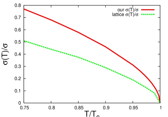
Figure 3: The ratio $\sigma(T)/\sigma$ at $N_{c}=2$ according to Eq. (6) (full drawn curve) and Ref. DFP (dashed curve).

Let us consider the limiting case when string bits cannot alter color, i.e. one should formally set in Eq. (6) $N_{c}=1$, that yields

$$\sigma(T)=\sigma+\sqrt{\frac{\sigma T}{a}}\left(1-\sqrt{\frac{T}{T_{0}}}\right).$$

The fundamental difference of this limiting case from the realistic one $N_{c}=3$ is that here $\sigma(T)\sim(T_{c}-T)$ at $T\to T_{c}$. The corresponding value of the critical exponent $\nu=1$ defines the universality class of the two-dimensional Ising model, which by no means can be realized in four-dimensional quenched SU($N_{c}$) QCD. The same linear fall-off of $\sigma(T)$ with $(T_{c}-T)$ one finds also in the Hagedorn phase transition and in the deconfinement scenario based on the condensation of long closed strings revs ; MO . It comes as a mere consequence of the formula $\sigma(T)=\sigma-\frac{TS}{R}$ with the entropy $S\propto R$. For long strings the entropy is just the logarithm of the number of possibilities to realize on a lattice with the spacing $a$ a closed trajectory of length $L$. Specifically for a hypercubic lattice, the entropy is $S=\frac{L}{a}\cdot\ln(2d-1)$. Therefore, the free energy of such a closed string, $F=\sigma L-TS$, vanishes at $T_{c}=\frac{\sigma a}{\ln(2d-1)}$. Numerically, in $d=4$ dimensions, $T_{c}=103{\,}{\rm MeV}$, that is by a large factor of 2.6 smaller than the modern lattice value 270 MeV. The principal difference of our calculation is that we consider the random walk between two different points, taking into account the confining force between the final and the initial points of the walk along its trajectory. These are the two facts, which eventually lead to a different critical behavior. In conclusion of this section, we note that the idea to have a large entropy of the $Q\bar{Q}$-string in the vicinity of $T_{c}$ due to the valence gluons has recently been mentioned in Ref. yuasim . However, the possibility that this mechanism leads to deconfinement has not been formulated in that paper.

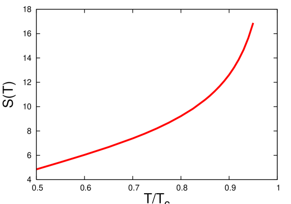
Figure 4: Entropy $S(T)$ of the static $Q\bar{Q}$-pair in the SU(2) quenched QCD at $R=1.5{\,}{\rm fm}$ and temperatures close to $T_{c}\simeq 304{\,}{\rm MeV}$, calculated from Eq. (6).

It should finally be mentioned that, in the string models discussed in the previous paragraph, as well as in the model developed in this paper, the free energy vanishes gradually at $T\to T_{c}$. Therefore, none of these models can describe first-order phase transition, which takes place in SU($N_{c}$) quenched QCD at $N_{c}\geq 3$. They only can describe the phase transition in the SU(2) quenched QCD, which was studied on the lattice in Ref. DFP . In that case, the mean-field critical exponent $\nu=1/2$, found in this paper and in Ref. pa , is changed to the 3d-Ising one, $\nu=0.63$. This makes our values of $\sigma(T)$ larger than those obtained in Ref. DFP . Using, similarly to that paper, the value $T_{c}=0.69\sqrt{\sigma}\simeq 304{\,}{\rm MeV}$, we plot in Fig. 3 the ratio $\sigma(T)/\sigma$ following from Eq. (6) at $N_{c}=2$. In the same figure, we present a curve interpolating the lattice data from Ref. DFP . In Figs. 4 and 5, we plot entropy and internal energy of the static $Q\bar{Q}$-pair in the SU(2) quenched QCD at $R=1.5{\,}{\rm fm}$, calculated from Eq. (6) by the formulae $S(T)=-R\frac{d\sigma(T)}{dT}$, $U(T)=\sigma(T)R+TS(T)$. These quantities read

$$S(T)=\sigma R\left[\frac{\beta}{2\sqrt{\sigma a(\beta-\beta_{c})}}+\beta_{c}-\sqrt{\frac{\beta-\beta_{c}}{\sigma a}}\right]\leavevmode\nobreak\ \leavevmode\nobreak\ {\rm and}\leavevmode\nobreak\ \leavevmode\nobreak\ U(T)=\sigma R\left[1+\frac{1}{2\sqrt{\sigma a(\beta-\beta_{c})}}\right],$$

respectively. In these equations, we use the value $\sigma a\simeq 0.21{\,}{\rm GeV}$, which stems from Eq. (7) upon the substitution $N_{c}=2$, $T_{c}=304{\,}{\rm MeV}$. This value of $\sigma a$ corresponds to $a\simeq 0.21{\,}{\rm fm}$, which is again larger than the vacuum correlation length in the SU(2) quenched QCD, $0.16{\,}{\rm fm}$ CDM . Both $S(T)$ and $U(T)$ have a singularity of the type $(T_{c}-T)^{-1/2}$ at $T\to T_{c}$. This singularity is weaker than $\delta\left(\frac{T_{c}-T}{T_{c}}\right)$, which takes place for the first-order phase transition at $N_{c}\geq 3$.

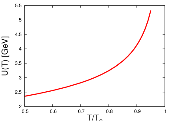
Figure 5: Internal energy $U(T)$ in GeV of the static $Q\bar{Q}$-pair in the SU(2) quenched QCD at $R=1.5{\,}{\rm fm}$ and temperatures close to $T_{c}\simeq 304{\,}{\rm MeV}$, calculated from Eq. (6).

III Static $Q\bar{Q}$-pair with light quarks at $T<T_{c}$

Let us now consider unquenched QCD with a heavy quark pair $Q\bar{Q}$ at large separation ($R\geq 1.5$ fm). Then the $Q\bar{Q}$-string breaks due to the production of a light $q\bar{q}$-pair. The subsequent hadronization process leads to the formation of a heavy-light meson ($\bar{Q}q$) or a heavy-light-light baryon ($Qqq$), together with their antiparticles. We will calculate the thermodynamics of these hadronic objects as a function of temperature. We consider the ($N_{f}=2$)-case, with light $u$- and $d$-quarks, and use the value $T_{c}=200{\,}{\rm MeV}$ given in tc in order to compare with the corresponding unquenched lattice simulations. Equation (7) then yields an effective value of $a=0.23{\,}{\rm fm}$, which is now used in Eq. (6) to determine $\sigma(T)$. For a heavy-light meson, the Hamiltonian of the relativistic $q\bar{Q}$-system is

$$H_{\bar{Q}q}=m_{\bar{Q}}+\sqrt{{\bf p}^{2}+m_{q}^{2}}+V(r)\leavevmode\nobreak\ \leavevmode\nobreak\ {\rm with}\leavevmode\nobreak\ \leavevmode\nobreak\ V(r)=\sigma(T)r-(2-\delta)\sqrt{\sigma(T)}.$$ (9)

The parameter $m_{\bar{Q}}$ denotes the heavy-antiquark mass, $m_{q}$ is the constituent mass of the light quark, $m_{q}\simeq 300{\,}{\rm MeV}$. The subtraction of $2\sqrt{\sigma(T)}$ in $V(r)$ is known to be important to reach agreement between the predictions of the relativistic quark model with the phenomenology of meson spectroscopy const2 ; const1 . An additional correction $\delta\sqrt{\sigma(T)}$ ensures that the mass of the lowest state in our calculation corresponds to the lightest heavy-quark meson. We use the $D^{0}$-meson with $m_{D^{0}}=1.864{\,}{\rm GeV}$ and $m_{\bar{Q}}=m_{c}=1.48{\,}{\rm GeV}$ to fix the parameters of our model.

The square root in the Boltzmann factor can be handled by integrating over an auxiliary parameter:

$$\exp\left(-\beta\sqrt{{\bf p}^{2}+m_{q}^{2}}\right)=\frac{2}{\sqrt{\pi}}\int_{0}^{\infty}d\mu\exp\left(-\mu^{2}-\frac{\beta^{2}}{4\mu^{2}}\left({\bf p}^{2}+m_{q}^{2}\right)\right).$$

One then arrives at a 3d Schrödinger equation of the form

$$(-K\vec{\nabla}^{2}+M|{\bf x}|)\psi({\bf x})=E\psi({\bf x}),$$

where $K$ and $M$ are positive constants of dimension $[{\rm length}]$ and $[{\rm mass}]^{2}$, respectively. Its eigenenergies read const2

$$E_{n_{r},l}=\alpha_{n_{r},l}\,(KM^{2})^{1/3},$$

where $\alpha_{n_{r},l}$’s are positive numbers with $\alpha_{00}\simeq 2.34$. In calculating the partition function of the heavy-light mesons $(\bar{Q}q$ and $Q\bar{q})$ const2 we take their ground state into account exactly and model their higher eigenenergies by those of a 3d harmonic oscillator with the frequency

$$\omega\equiv(KM^{2})^{1/3}=\left(\frac{\beta\sigma^{2}(T)}{4\mu^{2}}\right)^{1/3}.$$

This strategy works well for the lowest states, and higher states are Boltzmann-suppressed, so the lack of accuracy does not matter so much. Because of the degeneracy factor $(n/2+1)(n+1)$ for the oscillator, we have

$${\cal Z}_{{\rm 2mes}}=4{\cal Z}_{\bar{Q}q}^{2}\leavevmode\nobreak\ \leavevmode\nobreak\$$

with

$${\cal Z}_{\bar{Q}q}={2\over\sqrt{\pi}}\exp\left(-\beta m_{\bar{Q}}+(2-\delta)\beta\sqrt{\sigma(T)}\right)\times$$

$$\times\sum_{n=0}^{\infty}\left(\frac{n}{2}+1\right)(n+1)\int_{0}^{\infty}d\mu\exp\left[-(n+\alpha_{00})\beta\omega-\mu^{2}-\frac{\beta^{2}m_{q}^{2}}{4\mu^{2}}\right].$$ (10)

The partition function of two noninteracting mesons is $4{\cal Z}_{\bar{Q}q}^{2}$, where the factor 4 is a product of two flavors and two spin states of the mesons because the spins and isospins of the produced $q$ and $\bar{q}$ are coupled to isospin 0 and spin 0 by string breaking. The mass $m_{\bar{Q}}$ of the heavy antiquark is dropped in Eq. (10) in order to compare our calculation with the lattice data tc , which simulate a heavy quark and antiquark by two Polyakov lines. Doing the sum over $n$ analytically, we arrive at the following result:

$$F_{{\rm 2mes}}=-T\ln\frac{16}{\pi}-(4-2\delta)\sqrt{\sigma(T)}-2T\ln\Biggl{[}\int_{0}^{\infty}d\mu\exp\left(-\mu^{2}-\frac{\beta^{2}m_{q}^{2}}{4\mu^{2}}\right)\frac{\exp(-\alpha_{00}\beta\omega)}{(1-\exp(-\beta\omega))^{3}}\Biggr{]}.$$ (11)

The remaining $\mu$-integration is done numerically. The necessary value of the parameter $\delta$ to reproduce the correct $m_{D^{0}}$ mass is $\delta=0.354$, which can be obtained from the free energy $F$ in the limit $T\to 0$. Entropy and internal energy can be calculated by the standard formulae $S=-\partial F/\partial T$, $U=F+TS$. Note that, when calculating the entropy, the derivative $\partial/\partial T$ should not act on the Hamiltonian in the partition function, since otherwise the consistency of the thermodynamic relations would be violated.

It is also possible that string breaking generates a baryon and an antibaryon instead of two mesons. The Hamiltonian for a baryon reads

$$H_{Qqq}=m_{Q}+\sum\limits_{i=1}^{2}\left(\sqrt{{\bf p}_{i}^{2}+m_{q}^{2}}+V(r_{i})\right),$$

where we approximate the position of the baryon string junction by the position of the heavy quark $Q$, which is legitimate due to the heaviness of $Q$. Since the heavy quark $Q$ is static, terms from the two light quarks separate and one can deal with this Hamiltonian similar to the meson case. The corresponding free energy of baryon and antibaryon reads

$$F_{{\rm 2bar}}=-T\ln\frac{16}{\pi^{2}}-(8-4\delta)\sqrt{\sigma(T)}-4T\ln\Biggl{[}\int_{0}^{\infty}d\mu\exp\left(-\mu^{2}-\frac{\beta^{2}m_{q}^{2}}{4\mu^{2}}\right)\frac{\exp(-\alpha_{00}\beta\omega)}{(1-\exp(-\beta\omega))^{3}}\Biggr{]}.$$ (12)

For simplicity, we restrict ourselves to diquark quantum numbers with zero isospin and zero spin. The parameter $\delta$ in the baryon calculation is adjusted so that the corresponding ground state corresponds to the lightest charmed baryon $\Lambda_{c}^{+}$ with $m(\Lambda_{c}^{+})=2.286{\,}{\rm GeV}$. The resulting value $\delta=0.393$ is not very different from $\delta=0.354$ obtained for the heavy-meson system, therefore we use the averaged value $\delta=0.37$ in both cases.

Combining the contributions to the partition function coming from mesons and baryons, we have

$$F=-T\ln(Z_{\rm 2mes}+Z_{\rm 2bar})=-T\ln\left(4{\cal Z}_{\bar{Q}q}^{2}+{\cal Z}_{\bar{Q}q}^{4}\right).$$ (13)

In Figs. 6 and 7, we plot the entropy and the internal energy corresponding to Eq. (13) together with the corresponding lattice data  tc . Here $S(T)$ and $U(T)$ mean the change in entropy and internal energy due to the presence of a heavy quark-antiquark pair in the hadronic heat bath. The heat bath justifies the calculation in the canonical ensemble in our case. The heavy $Q$ and $\bar{Q}$ and the two light $q$ and $\bar{q}$ from string breaking are the sources of our mesons. Therefore we think that a comparison of our model calculation with the lattice simulation is appropriate. The agreement is very good for the entropy, while the internal energy coming from our calculations is smaller than the lattice results. Our curve is shifted downwards by $\Delta U\simeq-0.5{\,}{\rm GeV}$ compared with the lattice simulations. Due to the simplicity of our calculation the qualitative agreement is nevertheless good.

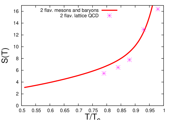
Figure 6: The calculated entropy $S(T)$ (full drawn curve) of two mesons and two baryons produced by string breaking for a heavy $Q$ and $\bar{Q}$ at large separation ($R\geq 1.5$ fm) is shown as a function of $T/T_{c}$ with $T_{c}=200$ MeV. The stars show the lattice data tc for the same $Q\bar{Q}$ configuration.

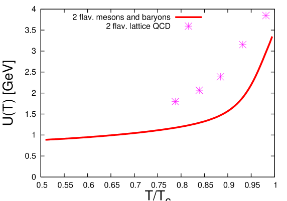
Figure 7: The calculated internal energy $U(T)$ (full drawn curve) of two mesons and two baryons produced by string breaking for a heavy $Q$ and $\bar{Q}$ at large separation ($R\geq 1.5$ fm) is shown as a function of $T/T_{c}$ with $T_{c}=200$ MeV. The stars show the lattice data tc for the same $Q\bar{Q}$ configuration.

IV Static $Q\bar{Q}$-pair with light quarks at $T>T_{c}$

In this section we consider a heavy $Q\bar{Q}$ pair at temperatures $T\geq T_{c}$, i.e. after deconfinement with free quarks and gluons present in the plasma. The heavy quark and antiquark are immersed into this plasma at the points ${\bf x}_{Q}$ and ${\bf x}_{\bar{Q}}$ at large separation ($R\geq 1.5$ fm). The non-Abelian interaction energy of a plasma constituent $a$ with the $Q\bar{Q}$ pair has the following form:

$${\cal V}^{a}({\bf r})=C^{aQ}{\cal U}(|{\bf r}-{\bf x}_{Q}|)+C^{a\bar{Q}}{\cal U}(|{\bf r}-{\bf x}_{\bar{Q}}|).$$ (14)

Here, $C^{aQ}$ and $C^{a\bar{Q}}$ are the corresponding color factors, namely products of SU(3) generators, which are discussed in Appendix B, and the interaction potential ${\cal U}({\bf r})$ is given by a screened gluon exchange between the colored sources

$${\cal U}({\bf r})=4\pi\int\frac{d^{3}{\bf k}}{(2\pi)^{3}}\frac{\alpha_{s}(k,T)}{k^{2}+m_{D}^{2}}{\rm e}^{i{\bf k}{\bf r}}.$$ (15)

For $\alpha_{s}$, we use a running coupling constant at finite temperature $T$ which has been derived in Ref. bpir ; bgies

$$\alpha_{s}(k,T) = \frac{u_{1}\frac{k}{T}}{1+\exp\left(u_{2}\frac{k}{T}-u_{3}\right)}+$$ (16)

$$+ \frac{v_{1}}{\left(1+\exp(v_{2}\frac{T}{k}-v_{3})\right)\ln\left({\rm e}+\left(\frac{k}{\Lambda_{s}}\right)^{a}+\left(\frac{k}{\Lambda_{s}}\right)^{b}\right)}.$$

This running coupling increases for small momenta $k$, has a maximum at $k\simeq T$ and finally decreases for $k\to\infty$.

The Debye mass is

$$m_{D}=\sqrt{\frac{N_{c}}{3}+\frac{N_{f}}{6}}\,\,gT\leavevmode\nobreak\ \leavevmode\nobreak\ \mbox{with}\leavevmode\nobreak\ \leavevmode\nobreak\ g=\sqrt{4\pi\alpha_{s}(m_{D},T)}\simeq 2.5.$$ (17)

This $g$ is determined from the selfconsistency equation bpir with the running coupling.

The interaction energy (14) is to be summed over all the $N$ constituents $a$ of the plasma, ${\cal V}({\bf r}_{1},\ldots,{\bf r}_{N})=\sum_{i=1}^{N}{\cal V}^{a_{i}}({\bf r}_{i})$. The perturbative expansion of the free energy in classical thermodynamics reads (see landau )

$$F=F_{0}+F_{Q\bar{Q}}+\langle{\cal V}({\bf r}_{1},\ldots,{\bf r}_{N})\rangle-{1\over 2T}\left(\langle{\cal V}^{2}({\bf r}_{1},\ldots,{\bf r}_{N})\rangle-\langle{\cal V}({\bf r}_{1},\ldots,{\bf r}_{N})\rangle^{2}\right),$$ (18)

where for each operator

$$\left<{\cal O}({\bf r}_{1},\ldots,{\bf r}_{N})\right>={\rm Tr}_{1}\left(\prod\limits_{i=1}^{N}\int\frac{d^{3}{\bf p}_{i}d^{3}{\bf r}_{i}}{(2\pi)^{3}}\right){\cal O}({\bf r}_{1},\ldots,{\bf r}_{N}){\rm e}^{\beta(F_{0}-E_{0})}.$$

Here, $F_{Q\bar{Q}}$ is the free energy of the interacting heavy $Q$ and $\bar{Q}$, $F_{0}$ is the free energy of the quark-gluon plasma, and the rest describes the interaction of the plasma constituents with the $Q\bar{Q}$-pair. Tr₁ denotes the trace over color indices of the interacting plasma constituent in the $Q\bar{Q}$ singlet state. The first-order term $\langle V({\bf r}_{1},\dots,{\bf r}_{N})\rangle$ vanishes due to color neutrality of the plasma, the second-order term, however, yields a nonvanishing result and describes the various interactions of the plasma constituents with the $Q\bar{Q}$ singlet state. The respective color factors can be calculated as products of generators in the various representations of SU(3). In second order, only the diagrams with two interactions of one plasma constituent with either $Q$ or $\bar{Q}$ or both of them are nonzero.

The energy of $N_{q}$ light quarks, $N_{\bar{q}}$ light antiquarks and $N_{g}$ gluons is $E_{0}=\sum^{N}_{i=1}\sqrt{{\bf p}_{i}^{2}+m_{i}^{2}}$, where $N=N_{q}+N_{\bar{q}}+N_{g}$. Here the squared mass of quarks and antiquarks is peshier ; lebellac

$$m_{q}^{2}=m_{\bar{q}}^{2}=m_{0}^{2}+2gT\sqrt{\frac{N_{c}^{2}-1}{16N_{c}}}\left(m_{0}+gT\sqrt{\frac{N_{c}^{2}-1}{16N_{c}}}\right)$$ (19)

and the kinetic mass of gluons is given by $m_{g}^{2}=\frac{1}{2}m_{D}^{2}$ peshier ; lebellac at $N_{c}=3$. We also use $g=2.5$ as above and set the current quark mass to $m_{0}=30$ MeV.

Although our heuristic introduction used classical statistics we will calculate in the following the free energy in quantum statistics as it is appropriate. The zeroth–order contribution $F_{0}$ reads

$$F_{0} = -\sum\limits_{a=q,\bar{q},g}N_{a}T\ln\left[\int d^{3}{\bf p}\,d^{3}{\bf r}\exp\left(-\beta\sqrt{{\bf p}^{2}+m_{a}^{2}}\right)\right]$$ (20)

$$= -\sum_{a}N_{a}T\ln\left(4\pi VTm_{a}^{2}K_{2}\left({m_{a}\over T}\right)\right),$$

where $K_{2}$ is a Macdonald function. The contribution $F_{0}$ of the quark-gluon plasma alone without the heavy $Q\bar{Q}$ pair is subtracted in lattice calculations lat ; tc . Therefore we will also leave it out in our results.

The contribution of the $Q\bar{Q}$-interaction,

$$F_{Q\bar{Q}}(R,T)=-\frac{4}{3}\alpha_{s}\frac{{\rm e}^{-m_{D}R}}{R},$$

can be neglected because it is of the order of a few MeV at large distances $R\simeq 1.5{\,}{\rm fm}$.

The term $\langle{\cal V}^{2}({\bf r}_{1},\ldots,{\bf r}_{N})\rangle$ in Eq. (18) is associated with two interactions of each plasma constituent. The contribution is the same for constituents of the same kind:

$$F_{2} = -{1\over 2T}\langle{\cal V}^{2}({\bf r}_{1},\ldots,{\bf r}_{N})\rangle$$ (21)

$$= -\frac{2}{\pi T}\left(\frac{2}{9}n_{q}^{{\rm eff}}+\frac{2}{9}n_{\bar{q}}^{{\rm eff}}+\frac{1}{2}n_{g}^{{\rm eff}}\right)\int d^{3}{\bf q}\frac{\alpha_{s}(q,T)^{2}}{(q^{2}+m_{D}^{2})^{2}}\left(1-{\rm e}^{i{\bf q}({\bf x}_{Q}-{\bf x}_{\bar{Q}})}\right)$$

(see Appendix C). In this equation, the color factors $c_{q}=c_{\bar{q}}=2/9$ and $c_{g}=1/2$ appear multiplying the effective densities $n_{a}^{{\rm eff}}=N_{a}^{{\rm eff}}/V$ of quarks, antiquarks or gluons, respectively. Since the heavy $Q\bar{Q}$ pair is color neutral, the contribution $F_{2}$ vanishes, when the $Q\bar{Q}$ - distance $|{\bf x}_{Q}-{\bf x}_{\bar{Q}}|$ approaches zero. The running of the coupling with temperature is crucial for the strong decrease of the entropy and internal energy with temperature. For a fixed value of $\alpha_{s}$ we would have

$$F_{2}=-\frac{1}{2T}\left(\frac{2}{9}n_{q}^{{\rm eff}}+\frac{2}{9}n_{\bar{q}}^{{\rm eff}}+\frac{1}{2}n_{g}^{{\rm eff}}\right)\alpha_{s}^{2}{4\pi\over m_{D}}\left(1-{\rm e}^{-m_{D}R}\right),\leavevmode\nobreak\ \leavevmode\nobreak\ R=|{\bf x}_{Q}-{\bf x}_{\bar{Q}}|=1.5{\,}{\rm fm},$$ (22)

and the corresponding entropy and internal energy would decrease with temperature even slower.

The next step is to calculate the effective densities, starting from the free ones. The particle densities of free quarks and gluons are listed in Appendix D, and the results are

$$n_{q} =n_{\bar{q}}=3TN_{f}\frac{m_{q}^{2}}{\pi^{2}}\sum_{n=1}^{\infty}\frac{(-1)^{n+1}}{n}K_{2}\left({m_{q}\over T}n\right),$$ (23)

$$n_{g} =12T\frac{m_{g}^{2}}{\pi^{2}}\sum_{n=1}^{\infty}\frac{1}{n}K_{2}\left({m_{g}\over T}n\right).$$

The full density is a sum of the three contributions $n_{q}+n_{\bar{q}}+n_{g}$. Confinement requires $n_{g,q,\bar{q}}^{\rm eff}(T_{c})=0$, therefore we add a factor $h(T)$ in the effective densities:

$$n^{{\rm eff}}_{a}(T)=h(T)n_{a}$$ (24)

with

$$h(T)=1-\exp\left(-\frac{T-T_{c}}{\lambda}\right).$$ (25)

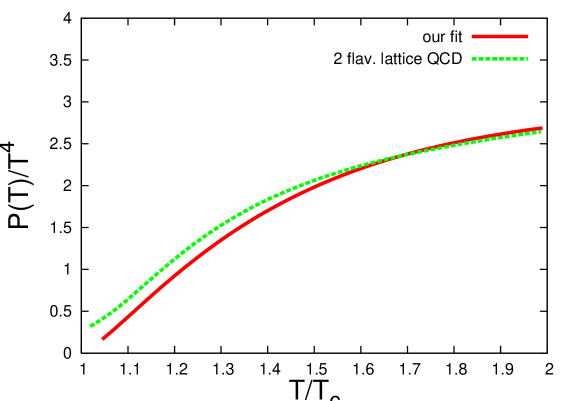
Figure 8: The calculated ratio $P_{{\rm eff}}(T)/T^{4}$ of Eq. (28) (full drawn curve) is shown in comparison with the one from lattice simulations of Ref. karsch (dashed curve) for two light flavors.

To obtain the parameter $\lambda=60$ MeV in $h(T)$, we have calculated the pressure corresponding to these effective densities and compared it with the pressure from lattice simulation in Ref. karsch . The grand canonical partition function from quarks, antiquarks and gluons has the form:

$$\ln Z_{\rm grand}=\sum_{a}D_{a}\frac{VTm_{a}^{2}}{2\pi^{2}}K_{2}\left({m_{a}\over T}\right).$$ (26)

Here, $D_{a}$ are the corresponding degeneracy factors, $D_{q}=D_{\bar{q}}=N_{c}N_{f}(2s_{q}+1)$ and $D_{g}=(N_{c}^{2}-1)N_{p}$ which contain $N_{p}=3$ as the number of polarizations of a massive gluon, and $s_{q}=1/2$ as the spin of the quark.

The pressure of free particles

$$P={T\over V}\ln Z_{\rm grand}=\frac{6T^{2}}{\pi^{2}}\left(2m_{g}^{2}K_{2}\left(\frac{m_{g}}{T}\right)+\frac{N_{f}}{2}m_{q}^{2}K_{2}\left({m_{q}\over T}\right)+\frac{N_{f}}{2}m_{\bar{q}}^{2}K_{2}\left({m_{\bar{q}}\over T}\right)\right)$$ (27)

would not vanish below $T_{c}$. To have a vanishing pressure at $T=T_{c}$, we also modify it by the confinement factor $h(T)$. Massless quarks and gluons have the density $n\propto T^{3}$ and the pressure $P\propto T^{4}$. Therefore, $P_{{\rm eff}}(T)$ is approximately suppressed by the factor $h(T)^{4/3}$:

$$P_{{\rm eff}}(T)=h(T)^{4/3}\cdot\frac{6T^{2}}{\pi^{2}}\left(2m_{g}^{2}K_{2}\left({m_{g}\over T}\right)+\frac{N_{f}}{2}m_{q}^{2}K_{2}\left({m_{q}\over T}\right)+\frac{N_{f}}{2}m_{\bar{q}}^{2}K_{2}\left({m_{\bar{q}}\over T}\right)\right).$$ (28)

In Fig. 8, we plot the ratio $P(T)/T^{4}$ from Ref. karsch and the ratio $P_{\rm eff}(T)/T^{4}$ from Eq. (28).

In the second-order free energy $F_{2}$, Eq. (22), we include the effective densities $n_{a}^{{\rm eff}}$, Eq. (24), modified by $h(T)$. In Fig. 9 and Fig. 10, we have plotted the entropy $S$ and the internal energy $U$ following from the standard thermodynamic relations $S(T)=-\partial F_{2}/\partial T$ and $U(T)=F_{2}(T)+TS(T)$ for two flavors. For the critical temperature we choose $T_{c}=$200 MeV for two flavors tc .

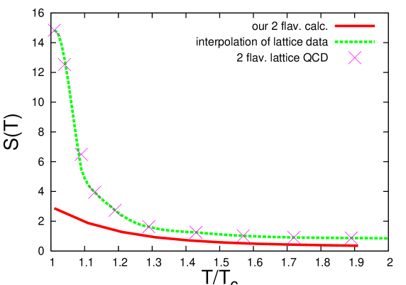
Figure 9: The calculated net entropy $S(T)$ at $N_{f}=2$ (full drawn curve) of a $Q\bar{Q}$ pair at large separation is shown as a function of $T/T_{c}$ with $T_{c}=200$ MeV. The entropy of the plasma without the $Q$ and $\bar{Q}$ pair is subtracted. Our calculation is compared with a function interpolating the lattice data tc ; lat (dashed curve) for better visibility.

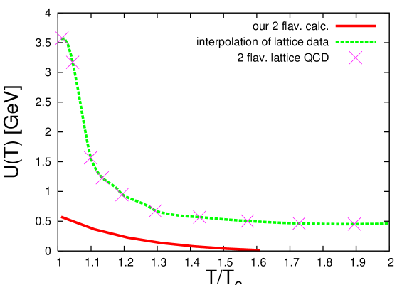
Figure 10: The calculated net internal energy $U(T)$ in GeV (full drawn curve) of a $Q\bar{Q}$ pair at large separation is shown as a function of $T/T_{c}$ with $T_{c}=200$ MeV. The internal energy of the plasma without the $Q$ and $\bar{Q}$ pair is subtracted. Our calculation is compared to a function interpolating the lattice data tc ; lat (dashed curve) for better visibility.

As one can see, $S(T)$ and $U(T)$ above $T_{c}$ are much smaller than in Refs. tc ; lat . We observe a difference $\Delta U\simeq-0.5{\,}{\rm GeV}$ for temperatures larger than $1.1T_{c}$ between our values of the internal energy and those of the lattice data, similarly to the result of the unquenched calculation at $T<T_{c}$. The trend from the lattice simulations that $S(T)$ and $U(T)$ decrease with $T$, is also seen here. For the case of three quark flavors, we show the results in Figs. 11, 12. The calculation of the entropy for three flavors is close to the one for two flavors. A similar result is obtained in the lattice simulations. However, there is one qualitative difference: Near $T_{c}$ two flavor lattice simulations give a larger $S(T)$ and $U(T)$ than simulations with three flavors. Our calculation yields opposite results. They arise from the flavor dependence of the densities and the Debye mass, which partially cancel and lead to an approximate independence of $S(T)$ and $U(T)$ on the number of flavors.

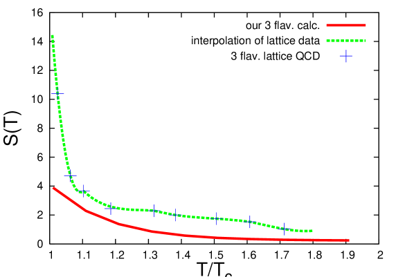
Figure 11: The calculated net entropy $S(T)$ at $N_{f}=3$ (full drawn curve) of a $Q\bar{Q}$ pair at large separation is shown as a function of $T/T_{c}$ with $T_{c}=193$ MeV. The entropy of the plasma without the $Q$ and $\bar{Q}$ pair is subtracted. Our calculation is compared with a function interpolating the lattice data tc ; lat (dashed curve) for better visibility.

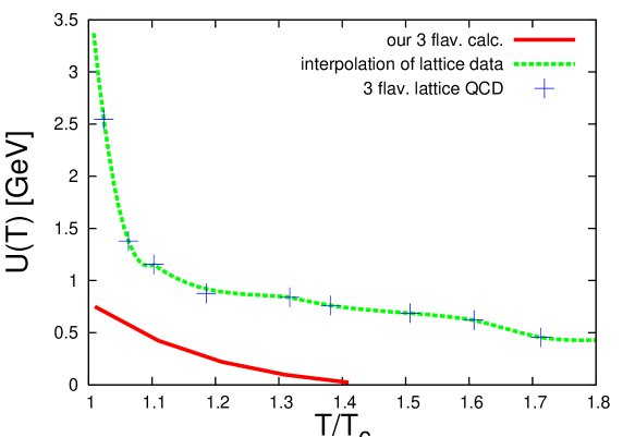
Figure 12: The calculated net internal energy $U(T)$ in GeV at $N_{f}=3$ (full drawn curve) of a $Q\bar{Q}$ pair at large separation is shown as a function of $T/T_{c}$ with $T_{c}=193$ MeV. The internal energy of the plasma without the $Q$ and $\bar{Q}$ pair is subtracted. Our calculation is compared to a function interpolating the lattice data tc ; lat (dashed curve) for better visibility.

We can enhance the internal energy and entropy by modifying our system in such a way that all quarks and antiquarks are bound in color-octet states and interact as such with the $Q\bar{Q}$-pair shu:bound . This yields an estimate for the influence of bound states on our calculations.

For simplicity we assume that the $q\bar{q}$ bound states have a mass of 2$m_{q}$. The corresponding degeneracy factor is now $(N_{c}^{2}-1)N_{f}^{2}N_{s}=16N_{f}^{2}$ ($N_{s}=2$ for spin 0 or 1). Therefore, the density is given as (cf. Eq. (23))

$$n_{q\bar{q}}=\frac{32}{\pi^{2}}TN_{f}^{2}m_{q}^{2}\sum_{n=1}^{\infty}\frac{1}{n}K_{2}\left(\frac{2m_{q}}{T}n\right).$$ (29)

As before, we obtain the effective density through the multiplication by $\widehat{h}(T)$, where the constant $\widehat{\lambda}$ is again fitted to reproduce the pressure, similarly to Eq. (28). This yields $\widehat{\lambda}=80$ MeV for two flavors. The color factor $c_{q\bar{q}}=1/2$ is the same as for gluons, and one can again determine entropy and internal energy from Eq. (21). These quantities are shown in Figs. 13 and 14.

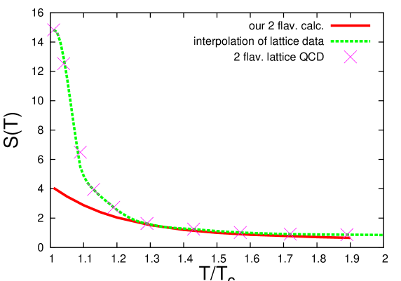
Figure 13: The calculated net entropy $S(T)$ (full drawn curve) of a $Q\bar{Q}$ pair at large separation interacting with $q\bar{q}$ bound states and gluons is shown as a function of $T/T_{c}$ with $T_{c}=200$ MeV. The entropy of the plasma without the $Q$ and $\bar{Q}$ pair is subtracted. Our calculation is compared to a function interpolating the lattice data tc ; lat (dashed curve) for better visibility.

In the vicinity of $T_{c}$ the entropy remains smaller than in the lattice calculations, but for higher temperatures it is in good agreement with the lattice data. In contrast, the internal energy is not very much different from the one without $q\bar{q}$ bound states. This shows that our calculation of the internal energy in second order perturbation theory is not changed very much by the presence of bound states in contrast to the otherwise shu:bound ; k:bound ; c:bound important effects of bound states in the quark-gluon plasma.

V Summary

In the present paper, we have analytically addressed the thermodynamics of a static quark-antiquark pair at large separation $R\geq 1.5$ fm in the vicinity of the deconfinement phase transition. In quenched QCD for $T<T_{c}$, the quark-antiquark string passes through valence gluons and forms a gluon chain. We have derived the resulting temperature-dependent string tension, Eq. (6), which vanishes at the critical point as $\sqrt{T_{c}-T}$. In unquenched QCD, for $T<T_{c}$ heavy-light mesons and heavy-light-light baryons are produced due to string breaking. The internal energy and entropy of our calculation fit quite well the corresponding lattice data. Finally, we have calculated the interaction energy for $T>T_{c}$ in unquenched QCD of the Debye-screened static quark-antiquark pair with the constituents of the plasma in second order thermodynamic perturbation theory. The change of the free energy depends on the effective density of quarks and gluons in the plasma, which has been constrained to vanish at $T=T_{c}$ and is adjusted in such a way that the pressure fits the one in lattice QCD for $N_{f}=2$. The entropy and internal energy of the model calculation differ from the lattice data. The large entropy near $T_{c}$ cannot be reproduced. The internal energies $U(T)$ calculated for the heavy $Q\bar{Q}$ pair are in both cases $T<T_{c}$ and $T>T_{c}$ by about 0.5–0.6 GeV lower than in the lattice simulations. The trend of a falling $S(T)$ and $U(T)$ with increasing $T$ is also seen in our model calculation. The heavy $Q\bar{Q}$-pair, immersed at large separation in the quark-gluon plasma, becomes less and less relevant at higher temperatures. Finally, the influence of possible $q\bar{q}$ bound states on our calculations has been estimated. Qualitatively, they do not change our results very much. If one wants to answer the question whether the hot QCD system is strongly interacting, our answer is twofold: Below $T_{c}$ the gluonic string and the excited hadronic states definitely represent strongly interacting composite systems. Above $T_{c}$ we have the screened color Coulomb-potential with its strength enhanced by the running QCD-coupling. The resulting calulated entropy, however, cannot fully reproduce the entropy from lattice simulations. At large temperatures the agreement becomes better. Surprisingly the internal energy of the simplified calculation and the lattice simulations do not converge. This divergence should be investigated more thoroughly.

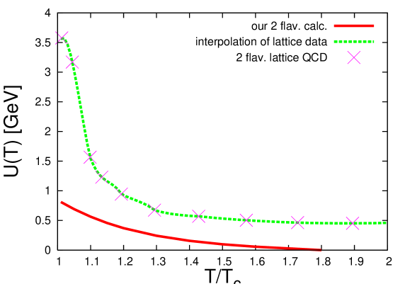
Figure 14: The calculated net internal energy $U(T)$ in GeV (full drawn curve) of a $Q\bar{Q}$ pair at large separation interacting with $q\bar{q}$ bound states and gluons is shown as a function of $T/T_{c}$ with $T_{c}=200$ MeV. The internal energy of the plasma without the $Q$ and $\bar{Q}$ pair is subtracted. Our calculation is compared to a function interpolating the lattice data tc ; lat (dashed curve) for better visibility.

Appendix A Computation of the sum for the three-dimensional harmonic oscillator

The sum over $n$ is computed by means of the formula

$$\sum_{n=0}^{\infty}n\exp(-\lambda\beta\omega n)=-{1\over\beta\omega}\frac{\mbox{d}}{\mbox{d}\lambda}\sum_{n=0}^{\infty}\exp(-\lambda\beta\omega n)=-{1\over\beta\omega}\frac{\mbox{d}}{\mbox{d}\lambda}\frac{1}{1-\exp(-\lambda\beta\omega)}$$ (30)

for the geometric series. Therefore, every factor of $n$ in the sum can be replaced by $-{1\over\beta\omega}\frac{d}{d\lambda}$, and we have

$$\sum_{n=0}^{\infty}\left(\frac{n}{2}+1\right)(n+1){\rm e}^{-\lambda\beta\omega n} = \left(\frac{1}{2(\beta\omega)^{2}}\frac{\mbox{d${}^{2}$}}{\mbox{d}\lambda^{2}}-\frac{3}{2\beta\omega}\frac{\mbox{d}}{\mbox{d}\lambda}+1\right)\sum_{n=0}^{\infty}{\rm e}^{-\lambda\beta\omega n}$$ (31)

$$= \frac{1}{\left(1-\exp(-\lambda\beta\omega)\right)^{3}}.$$

Appendix B Color factors

We shall discuss the color structure of the interaction term and the corresponding color factors here. As mentioned in the main text, the symbol $C^{aQ}$ carries the color indices of the interacting plasma constituent $a$ and both $Q$ and $\bar{Q}$. In the first order, the diagrams are proportional to Tr${}_{1}C^{aQ}$ (or Tr${}_{1}C^{a\bar{Q}}$, respectively), where $C^{aQ}$ is a product of the generators in the representations of the constituent $a$ and $Q$. For example, $C^{qQ}=t^{a}_{nm}t^{a\,Q}_{ji}\delta_{lk}$. Now, the effect of Tr₁ is that first order diagrams are proportional to the trace of the generator in the corresponding representation of the interacting constituent $a$, which vanishes. Therefore, first-order diagrams do not contribute.

For the relevant second order, we have squares of these color structures. Let us discuss this in more detail for one example and find the corresponding color factor. Therefore we consider a quark $q$ from the plasma, interacting two times with $Q$ and assume one-gluon-exchange (see Fig. 15).

Figure 15: Interaction of $q$ and $Q$ in second order

The color structure is

$$C_{ip\,lr\,mo}^{qQ}C_{pj\,rk\,on}^{qQ}=t^{a}_{om}t^{a\,Q}_{pi}\delta_{lr}t^{b}_{no}t^{b\,Q}_{jp}\delta_{rk},$$ (32)

where the indices $k$, $l$ and $p$ correspond to the $\bar{Q}$ which does not participate in this diagram. Furthermore, $t^{a}$ are the usual SU(3) generators in fundamental representation. With the use of $t^{a}_{ij}t^{a}_{kl}=1/2(\delta_{il}\delta_{jk}-1/3\delta_{ij}\delta_{lk})$ we can simplify this to

$$\frac{1}{2}\delta_{kl}\left(\frac{5}{9}\delta_{ij}\delta_{mn}-\frac{1}{3}\delta_{jm}\delta_{in}\right).$$ (33)

As we want to discuss only the $Q\bar{Q}$ singlet state here, we have to apply the projection operator phil

$$(P_{1}^{Q\bar{Q}})_{ji,lk}=\frac{1}{9}{\delta}_{ji}{\delta}_{lk}-\frac{2}{3}t^{a}_{ji}(-t^{a}_{lk})^{T}.$$ (34)

This yields the result $2/9\,\delta_{mn}$. A factor of 3, coming from the trace in Eq. (18), is taken into account for the densities (23). Therefore it should not be counted twice. There are other diagrams in second order, namely interaction of $q$ with $\bar{Q}$, $\bar{q}$ with $Q$ and $\bar{q}$ with $\bar{Q}$ which give the same result of 2/9. However, there are also diagrams, where a quark $q$ interacts with both $Q$ and $\bar{Q}$ or an antiquark interacts with both $Q$ and $\bar{Q}$. These diagrams have an odd number of interactions in the ${\bf\bar{3}}$ representation and therefore receive a relative minus sign.

For the gluons basically the same happens. There is one diagram containing two interactions of a gluon with $Q$ and the same for $\bar{Q}$. In addition, there are two diagrams for interactions both with $Q$ and $\bar{Q}$ which have a relative minus sign for the same reasons as above. As gluons are in adjoint representation, we have to use the corresponding generators. Let us again consider an example, where a gluon interacts twice with $Q$ (see Fig. 16).

Figure 16: Interaction of a gluon with $Q$ in second order

The color structure reads

$$C^{gQ}_{ir\,kp\,ac}C^{gQ}_{rj\,pl\,ce}=t^{b\,Q}_{ri}\delta_{kp}if^{bac}t^{d\,Q}_{jr}\delta_{pl}if^{dce}.$$ (35)

With the immediate use of the projection operator for the $Q\bar{Q}$ singlet state and the Casimir operator in adjoint representation $f^{abc}f^{ebc}=3\delta^{ae}$, one finally gets $1/2\delta_{ae}$. Again, the trace over color indices of the gluon was taken into account for the densities and should not be counted twice.

Diagrams which contain interactions of two plasma constituents do not contribute in second order because they are products of first-order diagrams which vanish.

Appendix C Calculation of the second order $F_{2}$

We now calculate the relevant second order for the free energy

$$F_{2}=-{1\over 2T}\langle{\cal V}^{2}({\bf r}_{1},\ldots,{\bf r}_{N})\rangle.$$ (36)

As we discussed before, only terms in the square which come from one plasma constituent $a$ contribute. This yields

$$\langle{\cal V}^{2}({\bf r}_{1},\dots,{\bf r}_{N})\rangle = \frac{1}{V}\sum_{i=1}^{N}c_{i}\int d^{3}{\bf r}_{i}\left[2\alpha_{s}^{2}\left(\frac{\exp(-m_{D}|{\bf r}_{i}-{\bf x}_{Q}|)}{|{\bf r}_{i}-{\bf x}_{Q}|}\right)^{2}\right.$$ (37)

$$\left.-2\alpha_{s}\frac{\exp(-m_{D}|{\bf r}_{i}-{\bf x}_{Q}|)}{|{\bf r}_{i}-{\bf x}_{Q}|}\alpha_{s}\frac{\exp(-m_{D}|{\bf r}_{i}-{\bf x}_{\bar{Q}}|)}{|{\bf r}_{i}-{\bf x}_{\bar{Q}}|}\right].$$

Here, $V$ is a three-dimensional volume (coming from $F_{0}$) which will be absorbed in the densities. While the first term comes from the Yukawa potential squared, the second term corresponds to the mixed term of the square. With the use of Fourier transformation, we can proceed to (${\bf d}_{i}={\bf r}-{\bf x}_{i}$)

$$-2(4\pi)^{2}\int d^{3}{\bf r}_{i}{d^{3}{\bf q}_{1}\over(2\pi)^{3}}{d^{3}{\bf q}_{2}\over(2\pi)^{3}}\alpha_{s}(q_{1},T)\frac{\exp(i{\bf q}_{1}{\bf d}_{Q})}{(q_{1}^{2}+m_{D}^{2})^{2}}\alpha_{s}(q_{2},T)\frac{\exp(i{\bf q}_{2}{\bf d}_{\bar{Q}})}{(q_{2}^{2}+m_{D}^{2})^{2}}$$ (38)

$$= -\frac{4}{\pi}\int d^{3}{\bf q}\alpha_{s}(q,T)^{2}\frac{\exp(i{\bf q}({\bf x}_{Q}-{\bf x}_{\bar{Q}}))}{(q^{2}+m_{D}^{2})^{2}}$$

for the second term and

$$2\int d^{3}{\bf r}_{i}\left(\alpha_{s}(|{\bf r}_{i}-{\bf x}_{Q}|,T)\frac{\exp(-m_{D}|{\bf r}_{i}-{\bf x}_{Q}|)}{|{\bf r}_{i}-{\bf x}_{Q}|}\right)^{2}$$ (39)

$$= \frac{4}{\pi}\int d^{3}{\bf q}\frac{\alpha_{s}(q,T)^{2}}{(q^{2}+m_{D}^{2})^{2}}$$

for the first one. The sum becomes trivial for each species of plasma constituents and can be written as $\sum_{a}c_{a}N_{a}^{{\rm eff}}$. With $N_{a}^{{\rm eff}}/V=n_{a}^{{\rm eff}}$ one can then introduce the densities here. Altogether we have

$$F_{2} = -{1\over 2T}\langle V^{2}({\bf r}_{1},\dots,{\bf r}_{N})\rangle$$ (40)

$$= -\frac{2}{\pi T}\sum_{a}c_{a}n_{a}^{{\rm eff}}\int d^{3}{\bf q}\frac{\alpha_{s}(q,T)^{2}}{(q^{2}+m_{D}^{2})^{2}}\left(1-{\rm e}^{i{\bf q}({\bf x}_{Q}-{\bf x}_{\bar{Q}})}\right).$$

Appendix D Computation of the density of free relativistic particles

We want to calculate the density of free relativistic particles for quarks (fermions) and gluons (bosons). It has the form

$$n_{a}=D_{a}\int{d^{3}{\bf p}\over(2\pi)^{3}}\frac{1}{\exp(\beta E_{0})\pm 1}$$ (41)

where $a$ stands for $q$, $\bar{q}$ or $g$, $E_{0}=\sqrt{{\bf p}^{2}+m_{a}^{2}}$, and $D_{a}$ is the degeneracy factor. Explicitly, this factor is $(N_{c}^{2}-1)N_{p}=8\cdot 3=24$ (due to color and polarization) for (massive) gluons and $N_{c}N_{f}(2s_{q}+1)=3\cdot N_{f}\cdot 2=6N_{f}$ (due to color, flavors and spin) for quarks.

Let us begin with quarks. The denominator can be rewritten by means of the geometric series:

$$\frac{1}{\exp(\beta E_{0})+1}=\frac{1}{\exp(\beta E_{0})}\frac{1}{1+\exp(-\beta E_{0})}={\rm e}^{-\beta E_{0}}\sum_{n=0}^{\infty}(-1)^{n}{\rm e}^{-\beta nE_{0}}.$$ (42)

Next, we can use the general formula

$$\int_{0}^{\infty}\frac{da}{\sqrt{\pi a}}{\rm e}^{-m^{2}a-\frac{R^{2}}{4a}}=\frac{{\rm e}^{-mR}}{m}$$ (43)

to obtain

$$n_{q} =12N_{f}\sum_{n=1}^{\infty}(-1)^{n+1}\int{d^{3}{\bf p}\over(2\pi)^{3}}{\rm e}^{-\beta nE_{0}}$$ (44)

$$=12N_{f}\sum_{n=1}^{\infty}(-1)^{n+1}\int{d^{3}{\bf p}\over(2\pi)^{3}}\int_{0}^{\infty}\frac{da}{\sqrt{\pi a}}\exp\left(-a-\frac{\beta^{2}n^{2}({\bf p}^{2}+m_{q}^{2})}{4a}\right).$$

The integral over ${\bf p}$ is now Gaussian and gives $\frac{1}{(2\pi)^{3}}\left(\frac{2\sqrt{\pi a}}{\beta n}\right)^{3}$. With the use of the formula

$$\int_{0}^{\infty}dtt^{\alpha-1}\exp\left(-\gamma t-{\delta\over t}\right)=2\left(\frac{\delta}{\gamma}\right)^{\alpha/2}K_{\alpha}(2\sqrt{\gamma\delta}),\leavevmode\nobreak\ \leavevmode\nobreak\ {\rm Re}{\,}\gamma>0,\leavevmode\nobreak\ \leavevmode\nobreak\ {\rm Re}{\,}\delta>0,$$ (45)

we get the final result

$$n_{q}=3N_{f}T\frac{m_{q}^{2}}{\pi^{2}}\sum_{n=1}^{\infty}\frac{(-1)^{n+1}}{n}K_{2}\left({m_{q}\over T}n\right).$$ (46)

The same result will appear for antiquarks, with $m_{\bar{q}}$ instead of $m_{q}$. For gluons (bosons) with the thermal mass $m_{g}$ the computation is nearly the same. Due to the minus sign in the denominator of (41), the factor $(-1)^{n}$ does not appear (and, of course, the factor of degeneracy is changed). We have

$$n_{g}=12T\frac{m_{g}^{2}}{\pi^{2}}\sum_{n=1}^{\infty}\frac{1}{n}K_{2}\left({m_{g}\over T}n\right).$$ (47)

References

- (1) K. Adcox et al. [PHENIX Collaboration], Nucl. Phys. A 757, 184 (2005)
- (2) I. Arsene et al. [BRAHMS Collaboration], Nucl. Phys. A 757, 1 (2005)
- (3) B. B. Back et al. [PHOBOS Collaboration], Nucl. Phys. A 757, 28 (2005)
- (4) J. Adams et al. [STAR Collaboration], Nucl. Phys. A 757, 102 (2005)
- (5) For a recent review see: E. V. Shuryak, The QCD vacuum, hadrons and superdense matter. 2nd edition, World Scientific (2004)
- (6) P. Arnold, G. D. Moore and L. G. Yaffe, JHEP 11, 001 (2000); ibid. 05, 051 (2003)
- (7) Yu. A. Simonov, Phys. Lett. B 619, 293 (2005)
- (8) P. Petreczky and K. Petrov, Phys. Rev. D 70, 054503 (2004)
- (9) P. Petreczky, Eur. Phys. J. C 43, 51 (2005)
- (10) K. J. Juge, J. Kuti and C. Morningstar, Nucl. Phys. Proc. Suppl. 63, 326 (1998); ibid. 73, 590 (1999); Phys. Rev. Lett. 82, 4400 (1999); ibid. 90, 161601 (2003)
- (11) N. Brambilla, A. Pineda, J. Soto and A. Vairo, Nucl. Phys. B 566, 275 (2000); Rev. Mod. Phys. 77, 1423 (2005); Yu. S. Kalashnikova and D. S. Kuzmenko, Phys. Atom. Nucl. 64, 1716 (2001); ibid. 66, 955 (2003)
- (12) J. Greensite and C. B. Thorn, JHEP 02, 014 (2002)
- (13) C. Itzykson and J.-M. Drouffe, Statistical field theory. Vol. 1, Cambridge Univ. Press (1989)
- (14) A. Di Giacomo and H. Panagopoulos, Phys. Lett. B 285, 133 (1992); M. D’Elia, A. Di Giacomo and E. Meggiolaro, Phys. Lett. B 408, 315 (1997); for a review see, e.g., A. Di Giacomo, "Nonperturbative QCD" [arXiv:hep-lat/9912016]; for the recent finite-temperature measurements see: M. D’Elia, A. Di Giacomo and E. Meggiolaro, Phys. Rev. D 67, 114504 (2003)
- (15) R. D. Pisarski and O. Alvarez, Phys. Rev. D 26 26, 3735 (1982)
- (16) See, e.g., H. Meyer-Ortmanns, Rev. Mod. Phys. 68, 473 (1996)
- (17) S. Digal, S. Fortunato and P. Petreczky, Phys. Rev. D 68, 034008 (2003)
- (18) M. Campostrini, A. Di Giacomo and G. Mussardo, Z. Phys. C 25, 173 (1984)
- (19) O. Kaczmarek and F. Zantow, Eur. Phys. J. C 43, 63 (2005); "Static quark anti-quark interactions at zero and finite temperature QCD. II: Quark anti-quark internal energy and entropy" [arXiv:hep-lat/0506019]
- (20) D. Gromes, "Theoretical understanding of quark forces", preprint HD-THEP-89-17
- (21) H. J. Pirner and M. Wachs, Nucl. Phys. A 617, 395 (1997) [arXiv:hep-ph/9701281]
- (22) J. Braun and H. J. Pirner, "Energy loss in the Quark-Gluon Plasma" [arXiv:hep-ph/0610331]
- (23) J. Braun and H. Gies, JHEP 06, 024, (2006)
- (24) L. D. Landau and E. M. Lifshitz, Statistical physics, Pergamon (1958)
- (25) M. Le Bellac, Thermal field theory, Cambridge Univ. Press (1996)
- (26) A. Peshier, B. Kämpfer, G. Soff, Phys. Rev. C 61, 045203 (2000)
- (27) F. Karsch, E. Laermann and A. Peikert, Phys. Lett. B 478, 447 (2000)
- (28) E.V. Shuryak, I. Zahed, Phys. Rev. D 70, 054507 (2004)
- (29) S. Datta, F. Karsch, P. Petreczky, I. Wetzorke, Phys. Rev. D 69, 094507 (2004); F. Karsch, Eur. Phys. J. C 43, 35 (2005)
- (30) N. Brambilla et al., "Heavy quarkonium physics" [arXiv:hep-ph/0412158]
- (31) O. Philipsen, Phys. Lett. B 535, 138 (2002)