Electromagnetic form factors of the nucleon in spacelike and timelike regions

Abstract

An approach for a unified description of the nucleon electromagnetic form factors in spacelike and timelike regions is presented. The main ingredients of our model are: $i)$ a Mandelstam formula for the matrix elements of the nucleon electromagnetic current; $ii)$ a $3$-dimensional reduction of the problem on the Light-Front performed within the so-called Propagator Pole Approximation (PPA), which consists in disregarding the analytical structure of the Bethe-Salpeter amplitudes and of the quark-photon vertex function in the integration over the minus components of the quark momenta; $iii)$ a dressed photon vertex in the $q\bar{q}$ channel, where the photon is described by its spin-$1$, hadronic component.

1 Introduction

The electromagnetic form factors of the nucleon represent a powerful tool to investigate the nucleon structure. In particular, a detailed knowledge of the responses of the nucleon to an electromagnetic probe can give useful information on the quark distributions inside the hadron state, together with an insight on the role played by the non-valence Fock components. Presently, the experimental investigation of the nucleon electromagnetic form factors poses various problems in both the spacelike (SL) and timelike (TL) regions. In particular, in the SL region the most striking observation is the discrepancy in the results obtained for the proton ratio $G_{E}^{p}(Q^{2})\mu_{p}/G_{M}^{p}(Q^{2})$ between the data collected by the Rosenbluth separation method and by the polarization transfer one [1]. As to the TL region, a sizable difference occurs between the theoretical expectations from perturbative QCD [2] - that predicts, at the threshold, a ratio $\left(\frac{G^{n}_{M}}{G^{p}_{M}}\right)^{2}\approx\left(\frac{q_{d}}{q_{u}}\right)^{2}\approx 0.25$ - and the experimental data by Fenice [3], where $G^{n}_{M}\approx G^{p}_{M}$. From such a perspective, a unified investigation of both SL and TL regions is well motivated.
In order to carry on the analysis for both these regions in the framework of the same Light-Front model, a reference frame with a non-vanishing plus component $q^{+}\neq 0$ is needed, otherwise no pair-production mechanism - fundamental in the TL region - is allowed. In view of this, we will adopt a reference frame where ${\bf q}_{\perp}=0$ and $q^{+}=\sqrt{|q^{2}|}$.

2 The Model

The starting point of our model is the covariant formula á la Mandelstam [4] for the nucleon electromagnetic current. In the SL region, where the process under investigation is the scattering $e^{-}N\rightarrow e^{-}N$, we describe the matrix elements of the macroscopic current

$$\langle N;\sigma^{\prime},P^{\prime}_{N}|j^{\mu}~{}|P_{N},\sigma;N\rangle=$$

$$=\bar{U}_{N}(P^{\prime}_{N},\sigma^{\prime})\left[-F_{2}(Q^{2}){{P^{\prime}_{N}}^{\mu}+{P_{N}}^{\mu}\over 2m_{N}}+\left(F_{1}(Q^{2})+F_{2}(Q^{2})\right)\gamma^{\mu}\right]U_{N}(P_{N},\sigma)$$

where the Dirac ($F_{1}$) and Pauli ($F_{2}$) nucleon form factors are present, by the following microscopical approximation:

$$\langle\sigma^{\prime},P^{\prime}_{N}|j^{\mu}~{}|P_{N},\sigma\rangle=3~{}N_{c}~{}\int{d^{4}k_{1}\over(2\pi)^{4}}\int{d^{4}k_{2}\over(2\pi)^{4}}\times$$

$$Tr_{\tau_{(1,2)}}~{}Tr_{\tau_{(3,N)}}~{}Tr_{\Gamma_{(1,2)}}~{}\left\{~{}\bar{\Phi}^{\sigma^{\prime}}_{N}(k_{1},k_{2},k^{\prime}_{3},P^{\prime}_{N})~{}S^{-1}(k_{1})~{}S^{-1}(k_{2})~{}{\cal I}^{\mu}_{3}~{}\times\right.$$

$$\left.~{}\Phi^{\sigma}_{N}(k_{1},k_{2},k_{3},P_{N})\right\}~{}.$$ (2)

Analogously, in the TL region we describe the annihilation matrix element $\langle N~{}\bar{N}|j^{\mu}|0\rangle$:

$$\langle N;\sigma^{\prime},P_{N}|j^{\mu}~{}|-P_{\bar{N}},\sigma;N\rangle=$$

$$=\bar{U}_{N}(P_{N},\sigma^{\prime})~{}\left[-F_{2}(q^{2}){{P_{N}}^{\mu}-{P_{\bar{N}}}^{\mu}\over 2m_{N}}+\left(F_{1}(q^{2})+F_{2}(q^{2})\right)~{}\gamma^{\mu}\right]~{}V_{N}(P_{\bar{N}},\sigma)$$

by a microscopical approximation given by:

$$\langle N;\sigma^{\prime},P_{N}|j^{\mu}~{}|-P_{\bar{N}},\sigma;N\rangle=3~{}N_{c}\int{d^{4}k_{1}\over(2\pi)^{4}}\int{d^{4}k_{2}\over(2\pi)^{4}}\times$$

$$Tr_{\tau_{(1,2)}}~{}Tr_{\tau_{(3,N)}}~{}Tr_{\Gamma_{(1,2)}}~{}\left\{\bar{\Phi}^{\sigma^{\prime}}_{N}(k_{1},k_{2},k^{\prime}_{3},P_{N})~{}S^{-1}(k_{1})~{}S^{-1}(k_{2})~{}{\cal I}_{3}^{\mu}~{}\times\right.$$

$$\left.\Phi^{\sigma}_{\bar{N}}(k_{1},k_{2},k_{3},-P_{\bar{N}})\right\}~{}.$$ (4)

In the previous expressions, $S(k)={(/\!\!\!\!k+m)/(k^{2}-m^{2}+\imath~{}\epsilon)}$ is the quark propagator, the quantity $\Phi^{\sigma}_{N}(k_{1},k_{2},k_{3},P_{N})$, with its Dirac-conjugate $\bar{\Phi}^{\sigma^{\prime}}_{N}(k_{1},k_{2},k^{\prime}_{3},P^{\prime}_{N})$, represents the nucleon Bethe-Salpeter amplitude (BSA), and ${\cal I}^{\mu}_{3}(k_{3},q)$ indicates the $q$-$\gamma$ vertex function, given by:

$${\cal I}^{\mu}_{3}(k_{3},q)=~{}\left({1+\tau_{z}\over 2}\right)~{}{\cal I}^{\mu}_{u}(k_{3},q)~{}+~{}\left({1-\tau_{z}\over 2}\right)~{}{\cal I}^{\mu}_{d}~{}(k_{3},q)=$$

$$={{\cal I}^{\mu}_{u}~{}+~{}{\cal I}^{\mu}_{d}\over 2}~{}+~{}\tau_{z}~{}{{\cal I}^{\mu}_{u}~{}-~{}{\cal I}^{\mu}_{d}\over 2}={\cal I}^{\mu}_{IS}(k_{3},q)+\tau_{z}{\cal I}^{\mu}_{IV}(k_{3},q)$$ (5)

where ${\cal I}^{\mu}_{u}$ (${\cal I}^{\mu}_{d}$) indicates the $u$ ($d$) quark contribution, while ${\cal I}^{\mu}_{IS}(k_{3},q)$ (${\cal I}^{\mu}_{IV}(k_{3},q)$) is the isoscalar (isovector) contribution.
To introduce a proper Dirac structure for the nucleon BSA, we describe the $qqq$-$N$ interaction through an effective Lagrangian, which represents an isospin-zero and spin-zero coupling for the (1,2) quark pair, as in Ref. [nua] but with $\alpha=1$. Then, the nucleon BSA is approximated as follows

$$\Phi^{\sigma}_{N}(k_{1},k_{2},k_{3},p)=\left[~{}S(k_{1})~{}\imath\tau_{y}~{}\gamma^{5}~{}S_{C}(k_{2})C~{}S(k_{3})~{}+~{}S(k_{3})~{}\imath\tau_{y}~{}\gamma^{5}~{}S_{C}(k_{1})\right.$$

$$\left.\times C~{}S(k_{2})~{}+~{}S(k_{3})~{}\imath\tau_{y}~{}\gamma^{5}~{}S_{C}(k_{2})C~{}S(k_{1})~{}\right]~{}\Lambda(k_{1},k_{2},k_{3})~{}\chi_{\tau_{N}}~{}U_{N}(p,\sigma)$$

(6)

where: i) $\Lambda(k_{1},k_{2},k_{3})$ describes the symmetric momentum dependence of the vertex function on the quark momentum variables, $k_{i}$, ii) $U_{N}(p,\sigma)$ is the nucleon Dirac spinor, iii) $\chi_{\tau_{N}}$ the nucleon isospin state and iv) $S_{C}(k)$ is the charge conjugate quark propagator.

Figure 1: Diagram (a) : valence, triangle contribution ($0<k_{i}^{+}<P^{+}_{N}$, $0<k_{3}^{+}+q^{+}<P^{+}_{N^{\prime}}$). Diagram (b) : non-valence contribution ($0>k_{3}^{+}>-q^{+}$). The symbol $\times$ on a quark line indicates a quark on the mass shell, i.e. $~{}k^{-}_{on}=(m^{2}+k^{2}_{\perp})/k^{+}$. (After Ref. [fb18]).

Figure 2: Diagrams contributing to the nucleon EM form factors in the timelike region. The solid circles represent the on-shell amplitudes, the solid squares represent the non-valence ones and the shaded circles represent the dressed photon vertex.

In order to apply phenomenological approximations inspired by the Hamiltonian language to our model, we need to project the matrix elements on the Light-Front. To this end, we integrate over the minus components of the quark momenta. We assume a suitable fall-off for the functions $\Lambda(k_{1},k_{2},k_{3})$ and $\Lambda(k_{1},k_{2},k^{\prime}_{3})$ appearing in the nucleon BSAs, to make finite the four dimensional integrations. Furthermore, we assume that the singularities of $\Lambda(k_{1},k_{2},k_{3})$ and $\Lambda(k_{1},k_{2},k^{\prime}_{3})$ give a negligible contribution to the integrations on $k_{1}^{-}$ and on $k_{2}^{-}$ and then these integrations are performed taking into account only the poles of the quark propagators.
The $k^{-}_{i}$ integrations automatically single out two kinematical regions, namely a valence region, given by a triangle process (Fig. 1 (a)), with the spectator quarks on their mass shell and both the initial and the final nucleon vertexes in the valence sector, and the non-valence region (Fig. 1 (b)), where the $q\bar{q}$ pair production appears and only the final nucleon vertex is in the valence sector. This latter term can be seen as a higher Fock state contribution of the nucleon final state to the form factors. According to this kinematical separation, both the isoscalar and the isovector part of the quark-photon vertex ${\cal I}^{\mu}_{3}$ contain a purely bare valence contribution and a contribution corresponding to the pair production ($Z$-diagram), which can be decomposed in a bare, point-like term and a vector meson dominance (VMD) term (Fig. 3):

$${\cal I}^{\mu}(k,q,i)={{\cal N}_{i}}~{}\theta(p^{+}-k^{+})~{}\theta(k^{+})\gamma^{\mu}+$$

$$+\theta({q}^{+}+k^{+})~{}\theta(-k^{+})\left[{Z_{b}~{}{\cal N}_{i}}~{}\gamma^{\mu}+Z_{V}\Gamma^{\mu}(k,q,i)\right]$$ (7)

with $i=IS,~{}IV$ and ${\cal N}_{IS}=1/6$, ${\cal N}_{IV}=1/2$. The first term in Eq. (7) is the bare coupling of the triangle contribution, while $Z_{b},~{}Z_{V}$ are renormalization constants to be determined from the phenomenological analysis of the data. As a consequence the SL form factors $F^{N}$ are the sum of a valence term, $F^{N}_{\Delta}$, plus a non-valence one, $F^{N}_{\cal{Z}}$.

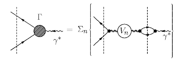
Figure 3: Diagrammatic analysis of the VMD contribution to the quark-photon vertex, $\Gamma^{\mu}(k,q)$. (After Ref. [plbpion]).

3 Phenomenological approximations

In order to overcome the lack of solutions for the $4$-dimensional Bethe-Salpeter equation in the baryon case, we insert in our model some phenomenological approximations. In particular, we test an Ansatz for the momentum dependent part $\Lambda(k_{1},k_{2},k_{3})$ of the nucleon BSA in Eq. (6), while the VMD description of the photon hadronic component, that appears in the quark-photon vertex, will be described by the eigenstates of a relativistic, squared mass operator introduced in Ref. [FPZ02].
In more details, the various amplitudes appearing in Figs. 1, 2 will be described as follows:

• for the solid circles, representing the valence, on-shell amplitudes, we adopt a power-law Ansatz á la Brodsky- Lepage [9];

• for the solid squares, representing the non-valence, off-shell amplitudes, we adopt a phenomenological form where the correlation between the spectator quarks is implemented;

• for the empty circle, representing a bare photon, a pointlike vertex, $\gamma^{\mu}$, is used;

• for the shaded circles, representing a dressed photon, we use the sum of a bare term and a microscopical VMD model [7].

The actual forms are the following. For the on-shell nucleon amplitude, we have:

$$\Psi_{N}(k^{+}_{1},{\bf k}_{1\perp},k^{+}_{2},{\bf k}_{2\perp},P_{N})=P_{N}^{+}\frac{\Lambda(k_{1},k_{2},k_{3})}{m_{N}^{2}-M_{0}^{2}}\sim{{\cal N}~{}P_{N}^{+}~{}{\cal F}(\xi_{1},\xi_{2},\xi_{3})\over\left[\beta^{2}+M^{2}_{0}(1,2,3)\right]^{3}}~{}~{}~{}~{}$$ (8)

where ${\cal F}(\xi_{1},\xi_{2},\xi_{3})$ is a symmetric scalar function depending on the momentum fraction carried by each constituent and $M_{0}(1,2,3)$ is the light-front free mass for the three-quark system. At the present stage we take ${\cal F}(\xi_{1},\xi_{2},\xi_{3})=1$. As to the non-valence amplitude, it is described by:

$$\Lambda(k_{1},k_{2},k_{3})\sim$$

$$\sim{{\cal G}(\xi_{1},\xi_{2},\xi_{3})\over\left[\beta_{off}^{2}+M^{2}_{0}(1,2)\right]^{p}}~{}\left\{{1\over\left[\beta_{off}^{2}+M^{2}_{0}(3^{\prime},2)\right]}+{1\over\left[\beta_{off}^{2}+M^{2}_{0}(3^{\prime},1)\right]}\right\}~{}~{}~{}~{}$$ (9)

where $M_{0}(i,j)$ is the light-front free mass for a two-quark system and ${\cal G}(\xi_{1},\xi_{2},\xi_{3})$ is a symmetric function of $\xi_{i}$. In this preliminary work ${\cal G}(\xi_{1},\xi_{2},\xi_{3})=1$ and $p=2$ are chosen. As to the $q$-$\gamma$ vertex, the term $\Gamma^{\mu}(k,q,i)$ in Eq. (7) is obtained through the same microscopical VMD model already used in the pion case with the same VM eigenstates [7]. Eventually, given the simplicity of the forms adopted for the nucleon amplitudes, a further dependence on the momentum transfer is introduced in the SL region through a modulation function $f(Q^{2})=(1+aQ^{2})/(1+bQ^{2})$, that parameterizes all the effects not included in the naïve amplitudes we are using. This function acts in the following way on the total form factors $F^{N}$: $F^{N}(Q^{2})=F^{N}_{\Delta}f^{2}(Q^{2})+F^{N}_{\cal{Z}}f(Q^{2})$.

4 Results and perspectives

  

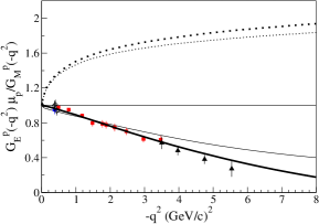
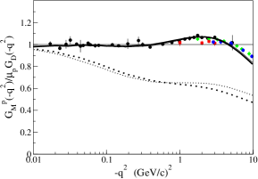
Figure 4: Left panel. The ratio $G^{p}_{E}(Q^{2})\mu_{p}/G^{p}_{M}(Q^{2})$ vs $Q^{2}$. Thin (thick) solid line: full calculation for a quark mass $m_{q}=190$ ($m_{q}=200$) MeV, corresponding to the sum of all the contributions to $G^{p}_{E}(Q^{2})$ and $G^{p}_{M}(Q^{2})$, i.e. triangle plus pair production terms. Thin (thick) dotted line: triangle elastic contribution to $G^{p}_{E}(Q^{2})$ and $G^{p}_{M}(Q^{2})$ for a quark mass $m_{q}=190$ ($m_{q}=200$) MeV. Right panel. $G^{p}_{M}(Q^{2})/\mu_{p}G_{D}(Q^{2})$ vs $Q^{2}$, with the same notations as in the left panel, and $G_{D}(Q^{2})=1/(1+Q^{2}/0.71)^{2}$. For experimental data see Ref. [JLAB2].

   

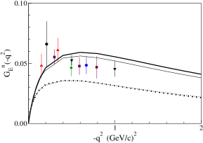
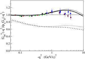
Figure 5: Left panel. $G^{n}_{E}(Q^{2})$ vs $Q^{2}$. Solid line: full calculation, corresponding to the sum of all the contributions to $G^{n}_{E}(Q^{2})$, i.e. triangle plus pair production terms. Dotted line: triangle elastic contribution to $G^{n}_{E}(Q^{2})$. Right panel. $G^{n}_{M}(Q^{2})/\mu_{n}G_{D}(Q^{2})$ vs $Q^{2}$ and $G_{D}(Q^{2})=1/(1+Q^{2}/0.71)^{2}$. The notation is the same as in Fig. 4. For experimental data see Ref. [JLAB2].

  

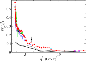
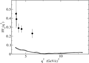
Figure 6: Left Panel. Proton effective form factor in the timelike region. Thin (thick) solid line: calculation for a quark mass $m_{q}=190$ ($m_{q}=200$) MeV. For the experimental data see Ref. [babar] and Refs. therein. Right Panel. Neutron effective form factor in the TL region, with the same notation of the Left Panel. Data by Fenice Collaboration[3].

The preliminary results obtained with our model are reported in Figs. 4, 5 and 6. They show clearly the relevant role played by the pair production process - and then by the non-valence components - for the nucleon form factors. In particular, the interplay between the valence and non-valence contributions generates the possibility to have a zero in the proton electric form factor. A reasonable description of the experimental data in the SL region is obtained, with a modulation factor $f(Q^{2})$ which grows from 1 to 1.08, at most. As to the TL region, our preliminary results reproduce the behavior of the experimental data, but for a scale factor.
Various improvements can be applied to our model. First of all, a more elaborate form for the nucleon non-valence amplitude - that is tested for the first time in this model - could allow for a better description of the experimental data in the TL region. Another improvement can derive from a better description of the quark-photon vertex, and in particular for the VMD approximation. A new, fully covariant VMD model is presently under investigation.

References

• [1] J. Arrington, Phys. Rev. C 68 (2003) 034325.
• [2] J. Ellis, M. Karliner, New J. Phys. 4 (2002) 18.
• [3] Fenice Collaboration, Nucl. Phys. B 517, 3 (1998).
• [4] S. Mandelstan, Proc. Royal Soc. (London) A233, 248 (1956).
• [5] W.R.B. de Araújo, E.F. Suisso, T. Frederico, M. Beyer and H.J. Weber, Phys. Lett. B 478, 86 (2000); Nucl. Phys. A 694, 351 (2001).
• [6] E. Pace, G. Salmè, T. Frederico, S. Pisano and J.P.B.C. de Melo, hep-ph/0607342, hep-ph/0611328.
• [7] J.P.B.C. de Melo, T. Frederico, E. Pace and G. Salmè, Phys. Lett. B 581, 75 (2004); Phys. Rev. D 73, 074013 (2006).
• [8] T. Frederico, H.-C. Pauli and S.-G. Zhou, Phys. Rev. D66, 054007 (2002); ibidem D66, 116011 (2002).
• [9] G. P. Lepage and S. J. Brodsky, Phys. Rev. D22, 2157 (1980).
• [10] www.jlab.org/ cseely/nucleons.html and Refs. therein.
• [11] BaBar Collaboration, Phys. Rev. D 73, 012005 (2006).