On the ”toy model” in the Reggeon Field Theory

Abstract

The Reggeon field theory with zero transverse dimensions is studied in the Hamiltonian formulation for both sub-and supercritical pomeron. Mathematical aspects of the model, in particular the scalar products in the space of quantum states, are discussed. Relation to reaction-diffusion processes is derived in absence of pomeron merging. Numerical calculations for different parameters of the models, $\alpha(0)-1=\mu$ and the triple pomeron coupling constant $\lambda$, show that the triple pomeron interaction always makes amplitudes fall with rapidity irrespective of the value of the intercept. The smaller the values of the ratio $\lambda/\mu$ the higher are rapidities $y$ at which this fall starts, so that at small values of $\lambda$ it begins at asymptotically high rapidities (for $\lambda/\mu<1/4$ the fall is noticeable only at $\mu y>100$). No visible singularity is seen for the critical pomeron. A perturbative treatment is proposed which may be useful for more realistic models.

1 Introduction

At high energies the Quantum Chromodynamics tells us that particle interaction may be mediated by the exchange of hard pomerons, which are non-local entities propagating according to the BFKL equation and splitting into two or merging from two to one with the known triple pomeron verteces. This most complicated picture can be drastically simplified in the quasi-classical treatment supposedly valid when at least one of the colliding hadrons is a heavy nucleus. This leaves only tree diagrams which can be summed by comparatively simple equations, which at least admit numerical solution. However at present much attention is drawn to the contribution of loops. This is obviously a problem of a completely different level of complexity, since it amounts to solving a full-fledged non-local quantum field theory. At present a solution of even some local quantum field theory has not been known except for the one-dimensional case. Naturally for the study of loops in QCD an one-dimensional model has been lately chosen as a starting point.

The one-dimensional (”toy”) model for the QCD interaction was proposed and solved by A.H.Mueller  [1]. However much earlier a model similar in structure was studied in the framework of a local Reggeon field theory (RFT) with a supercritical pomeron and imaginary triple pomeron interaction in a whole series of papers  [2, 3, 4, 5, 6, 7] As expected the one-dimensional reduction of the RFT admitted more or less explicit solution and lead to definite predictions as to the behaviour of amplitudes both for hA and AB interaction (of course with the understanding of a highly artificial physical picture, very far from the realistic world). In the course of study many ingeneous tricks and techniques were employed and the underlying complicated dynamics was revealed. However some subtle points have remained unclear in our opinion. In particular the nature of correspondence between the functional and Hamiltonial approaches and the origin of restrictions on the form of wave function and the range of its variable have not been fully exposed.

To elucidate these points is the primary aim of this note. We also try to follow the line presented in  [8, 9] to relate the RFT with the probabilistic parton picture and the so-called reaction-diffusion model for the case when there is no merging of pomerons (fan diagrams). This gives us a possibility to find the contribution from the loops with the highest extention in rapidity just by joining two fans propagating from the projectile and target towards the center. We additionally develop a perturbation theory for small $\lambda$ to compute the evolution by noting the PT-symmetry of the model. We finally report on some numerical results on solving the RFT with all loops, which can be obtained quite easily by integrating the corresponding evolution equations.

Note that we study exclusively a model with the triple pomeron interaction only. A different model which additionally includes a quartic pomeron interaction with a particular fine-tuned value of the coupling constant has lately received enough attention in literature  [8, 9, 10, 11]. In our opinion the quartic interaction has no immediate counterpart in the realistic pomeron theory with a large number of colours $N_{c}$, where it is damped by factor $1/N_{c}^{2}$.

2 Functional integral formulation

The toy model of Pomeron interaction with a zero-dimension transverse space can be defined by a generating functional

$$Z=\int D\phi D\phi^{\dagger}e^{-S},$$ (1)

where

$$S=\int dy{\cal L},\ \$$ (2)

and

$${\cal L}=\frac{1}{2}(\phi^{\dagger}\phi_{y}-\phi^{\dagger}_{y}\phi)-\mu\phi^{\dagger}\phi+i\lambda\phi^{\dagger}\phi(\phi^{\dagger}+\phi)-i(j_{0}\,\phi^{\dagger}+j_{Y}\,\phi).$$ (3)

Here $\mu$ is the pomeron intercept ($\alpha(0)-1$). For the supercritical pomeron $\mu>0$. Triple pomeron coupling constant $\lambda$ is also positive. The sources $j_{0}=\delta(y)g_{1}$ amd $j_{Y}=\delta(y-Y)g_{2}$ represent the interaction with the target and projectile respectively. In the real world $g_{1}=g_{1}(b)=AgT_{A}(b)$ and $g_{2}=g_{2}(b)=BgT_{B}(b)$ where $g$ is the pomeron-nucleon coupling constant, $A$ and $B$ are atomic numbers of the colliding nuclei and $T_{A}$ and $T_{B}$ their profile functions.

The functional integral (1) converges for $\mu<0$ provided the two field variables $\phi$ and $\phi^{\dagger}$ are complex conjugate to one another. In fact putting $\phi=\phi_{1}+i\phi_{2}$ and $\phi^{\dagger}=\phi_{1}-i\phi_{2}$, with both $\phi_{1,2}$ real, we find that all terms in the Lagrangian (3) are pure imaginary except for the mass term proportional to

$$\phi^{\dagger}\phi=\phi_{1}^{2}+\phi_{2}^{2}\geq 0.$$

So the integrand in (1) contains a factor $\exp\Big{(}\mu\int dy(\phi_{1}^{2}+\phi_{2}^{2})\Big{)}$, which guarantees convergence if $\mu<0$ and the integration over the fields $\phi_{1}$ and $\phi_{2}$ goes over the real axis. For $\mu>0$ the integral does not exist. Note that the integral does not exist for any sign of $\mu$ either, if one changes the integration contour in $\phi_{1}$ and $\phi_{2}$ and so over $\phi$ and $\phi^{\dagger}$. This means that it is impossible to pass to new fields $u=i\phi^{\dagger}$ and $v=i\phi$ and take $u$ and $v$ real directly in the functional integral as in  [3], since it requires unlawful rotation of the integration contour in the integration over $\phi_{1}$.

Obviously the functional formulation can serve only to define the model for the subcritical pomeron with $\mu<0$. To define the theory for positive values of $\mu$ one has to recur to analytic continuation in $\mu$. Note that the properties of the functional integral make one think that there is a singularity at $\mu=0$. In a fully dimensional RFT it was conjectured that this singularity was related to a phase transition. However already in  [6] it was argued that there was no phase transition in the zero-dimensional world and the amplitudes were analytic in $\mu$ on the whole real axis. As we shall see by direct numerical calculation, there is indeed no singularity at $\mu=0$ in scattering amplitides.

In fact the functional formulation is only supported by the fact that it reproduces the perturbative diagrams for the pomeron propagation and interaction. In the following section we introduce an alternative, Hamiltonian formalism, which gives rise to the same perturbative diagrams (such an approach as a starting point was briefly mentioned in  [4]). However in contrast to the functional approach it does not involve any limitation on the value or sign of the intercept $\mu$. Since for $\mu<0$ the perturbative series seems to be convergent, the two formulations are completely equivalent for the subcritical pomeron. Therefore the Hamiltonian formulation gives the desired analytic continuation of the model to positive values of $\mu$.

3 Hamiltonian formulation

3.1 Basic definitions

Forgetting the functional integral (1) altogether, we now start from a quasi-Schroedinger equation in rapidity:

$$\frac{d\Psi(y)}{dy}=-H\Psi(y)$$ (4)

and postulate the form of the Hamiltonian $H$

$$H=-\mu\phi^{\dagger}\phi+i\lambda\phi^{\dagger}(\phi+\phi^{\dagger})\phi$$ (5)

as a function of two Hermithean conjugate operators $\phi$ and $\phi^{\dagger}$ with the commutator

$$[\phi,\phi^{\dagger}]=1.$$ (6)

The Hamiltonian is obviously non-Hermithean. We standardly split it into a free and interaction parts:

$$H=H_{0}+H_{I},\ \ H_{0}=-\mu\phi^{\dagger}\phi,\ \ H_{I}=i\lambda\phi^{\dagger}(\phi+\phi^{\dagger})\phi.$$ (7)

Next step is to define physical observables in this picture. In accordance with the commutation relation (66) we define the vacuum state $\Psi_{0}$, normalized to unity, by the condition

$$\phi\Psi_{0}=0.$$ (8)

All other states will be built from $\Psi_{0}$ by application of some number of operators $\phi^{\dagger}$. We postulate that the transition amplitude from the initial state $\Psi_{i}$ at rapidity $y=0$ to the final state $\Psi_{f}$ at rapidity $y$ is given by

$$iA_{fi}=\langle\Psi_{f}|\Psi_{i}(y)\rangle=\langle\Psi_{f}|e^{-Hy}|\Psi_{i}\rangle.$$ (9)

Here

$$\Psi_{i}(y)=e^{-Hy}\Psi_{i}$$ (10)

is the initial state evolved to rapidity $y$. The amplitude $A_{fi}$ is imaginary positive so that the matrix element on the right-hand side of (9) is negative.

It will be convenient to define the initial and final states in terms of some operators acting on the vacuum state:

$$\Psi_{i}=F_{i}(\phi^{\dagger})\Psi_{0},\ \ \Psi_{f}=F_{f}(\phi^{\dagger})\Psi_{0}.$$ (11)

This allows to rewrite the amplitude as a vacuum average

$$iA_{fi}=\langle F_{f}^{*}(\phi)e^{-Hy}F_{i}(\phi^{\dagger})\rangle,$$ (12)

where we do not explicitly write the vacuum state $\Psi_{0}$ in which the average is taken.

3.2 Perturbative expansion

We are going to prove that the perturbative expansion of this theory leads to the same Feynman diagrams as from the functional approach. To this end we present

$$iA_{fi}=\langle e^{H_{0}y}F_{f}^{*}(\phi)e^{-H_{0}y}e^{H_{0}y}e^{-Hy}F_{i}(\phi^{\dagger})\rangle.$$ (13)

From (6) it follows that

$$\phi(y)\equiv e^{H_{0}y}\phi e^{-H_{0}y}=e^{\mu y}\phi.$$ (14)

The operator

$$U(y)\equiv e^{H_{0}y}e^{-Hy}$$ (15)

satisfies the equation

$$\frac{dU(y)}{dy}=e^{H_{0}y}(H_{0}-H)e^{-H(y)}=-e^{H_{0}y}H_{i}e^{-H_{0}y}U(y)=H_{I}(y)U(y),$$ (16)

where $H_{I}(y)$ is the interaction in the interaction representation:

$$H_{I}(y)=e^{H_{0}y}H_{I}(\phi,\phi^{\dagger})e^{-H_{0}y}=H_{I}(\phi(y),\phi^{\dagger}(y)),$$ (17)

with the rapidity dependent operators (14) and

$$\phi^{\dagger}(y)\equiv e^{H_{0}y}\phi^{\dagger}e^{-H_{0}y}=e^{-\mu y}\phi^{\dagger}.$$ (18)

Note that at $y>0$ the operators $\phi(y)$ and $\phi^{\dagger}(y)$ are no more Hermithean conjugate to each other, since the normal time is changed to the imaginary one. However the similarity transformations (14) and (18) do not change the commutation relations. The solution of (16) with the obvious initial condition $U(0)=1$ is standard

$$U(y)=T_{y}\exp\Big{\{}-\int_{0}^{y}dy^{\prime}H_{i}(y^{\prime})\Big{\}},$$ (19)

where $T_{y}$ means ordering the operators from left to right according to decreasing $y$’s. So we get the expression for the amplitude as

$$iA_{fi}=\langle F^{*}_{f}(e^{\mu y}\phi)T_{y}\exp\Big{\{}-\int_{0}^{y}dy^{\prime}H_{i}(y^{\prime})\Big{\}}F_{i}(\phi^{\dagger})\rangle.$$ (20)

Expansion of the $T_{y}\exp$ gives rise to standard Feynman diagrams. Verteces for pomeron splitting and merging will be given by the expected factors $i\lambda$. The pomeron propagator will be given by

$$P(y_{1}-y_{2})=\langle T_{y}\Big{\{}\phi(y_{1}),\phi^{\dagger}(y_{2})\Big{\}}\rangle=e^{\mu(y_{1}-y_{2})}\theta(y_{1}-y_{2}),$$ (21)

which is the correct pomeron propagator in our toy model. So indeed the theory defined by this Hamiltonial formulation gives rise to standard Feynman diagrams for the RFT.

Note that the Hamiltonian formulation is based on the evolution equation in rapidity and does not require the intercept $\mu$ to have a definite sign. It looks equally good both for positive and negative values of $\mu$. For negative $\mu$ it produces a perturbative expansion which is identical to that in the functional approach. So it gives the desired analytic continuation of the functional approach to the region of positive $\mu$, where the latter looses sense.

3.3 Passing to a real Hamiltonian

It is perfectly possible to continue with the originally defined Schroedinger operators $\phi$ and $\phi^{\dagger}$ which are Hermithean conjugate to each other and satisfy the commutation relation (6). However it is convenient to pass to new operators $u$ and $v$ in terms of which all ingredients of the theory become real. Following the old papers (starting from  [2]) we define

$$u=i\phi^{\dagger},\ \ v=i\phi.$$ (22)

The new fields are anti-Hermithean to each other

$$u^{\dagger}=-v,\ \ v^{\dagger}=-u$$ (23)

and satisfy the commutation relation

$$[v,u]=-1.$$ (24)

However $v\Psi_{0}=0$ and the states are generated by action of $u$. So $v$ is the annihilation and $v$ is the creation operator with abnormal commutation relation (24).

In terms of new fields the Hamiltonian becomes real

$$H=\mu uv-\lambda u(u+v)v.$$ (25)

It is important that also the operators creating the initial and final states become real. It is normally assumed that for the scattering of two nuclei the initial and final wave functions should correspond to the eikonal picture. In terms of creation operator $u$ this leads to

$$\Psi_{i(f)}=F_{i(f)}(u)\Psi_{0},\ \ F_{i(f)}(u)=1-e^{-g_{i(f)}u}.$$ (26)

So the expression for the amplitude is rewritten in terms of real quantities:

$$iA_{fi}=\langle F_{f}(u)\Psi_{0}|e^{-Hy}|F_{i}(u)\Psi_{0}\rangle=\langle\Psi_{0}|F^{*}_{f}(-v)e^{-Hy}F_{i}(u)\Psi_{0}\rangle$$

$$=\langle\Big{(}1-e^{-g_{f}v}\Big{)}e^{-Hy}\Big{(}1-e^{-g_{i}u}\Big{)}\rangle.$$ (27)

Since $H\Psi_{0}=0$ the term independent of $g_{i}$ and $g_{f}$ vanishes, so that we can also write

$$iA_{fi}=-\langle e^{-g_{f}v}e^{-Hy}\Big{(}1-e^{-g_{i}u}\Big{)}\rangle=-\langle\Psi_{0}|e^{-g_{f}v}F_{i}(y,u)\Psi_{0}\rangle,$$ (28)

where $F_{i}(y,u)$ is the operator which creates the evolved initial state. Since

$$\Psi_{i}(y)=e^{-Hy}\Psi_{i}=e^{-Hy}F_{i}(u)\Psi_{0}\equiv F_{i}(y,u)\Psi_{0},$$ (29)

we have

$$\frac{\partial F_{i}(y,u)}{\partial y}=-H(u,v)F_{i}(y,u)$$ (30)

with an initial condition

$$F_{i}(0,u)=1-e^{-g_{i}u}.$$ (31)

The commutation relation (24) allows to represent

$$v=-\frac{\partial}{\partial u}$$ (32)

and then (28) implies that to find the amplitude one has to substitute $u$ by $g_{f}$ in $F_{i}(y,u)$

$$iA_{fi}=-F_{i}(y,g_{f}).$$ (33)

This gives a practical recipe for the calculation of the amplitude. One has to solve Eq. (30) with the Hamiltonian (25) in which $v$ is represented according to (32):

$$H=-\mu u\frac{\partial}{\partial u}+\lambda u^{2}\frac{\partial}{\partial u}-\lambda u\frac{\partial^{2}}{\partial u^{2}}$$ (34)

and the initial condition (31). After the solution is found, one has to substitute $u$ by $g_{f}$ in it.

3.4 Target-projectile symmetry

Taking the complex conjugate of (28) we find

$$-iA^{*}_{fi}=\langle\Big{(}1-e^{g_{i}v}\Big{)}e^{-H^{\dagger}y}\Big{(}1-e^{g_{f}u}\Big{)}\rangle=iA_{if}(\lambda\to-\lambda,g_{i(f)}\to-g_{f(i)}).$$ (35)

Having in mind that the amplitude is pure imaginary, we see that interchanging the target and projectile leads to changes of sign in the triple pomeron coupling and the couplings to the external particles. On the other hand changing $u\to-u$ in Eq. (30) with the Hamiltonian (34) and the initial condition (31) and also changing signs of $\lambda$ and $g_{i}$ obviously does not change the solution:

$$F_{i}(y,-u,-g_{i},-\lambda)=F_{i}(y,u,g_{i},\lambda),$$ (36)

from which we find

$$F_{i}(y,-g_{f},-g_{i},-\lambda)=F_{i}(y,g_{f},g_{i},\lambda).$$ (37)

So the interchange of the target and projectile does not change the amplitude.

3.5 Scalar products

As follows from our derivation the exact mathematical realization of the scalar product in the space of wave functions $\Psi$ is irrelevant for the resulting formulas. The representation of the operator $v$ as a minus derivative in $u$ serves only to express its algebraic action on the operator $u$ in accordance with the commutation relation. It does not require to introduce a representation for the wave function $\Psi$ in which $u$ is represented as multiplication by a complex number and correspondingly the scalar product is defined by means of integration over the whole complex plane $u$ with a weight factor $e^{-uu^{*}}$ aas in  [6]. One may instead represent operators $u$ and $v$ in terms of the standard Hermithean operators $p$ and $q$ as

$$u=\frac{i}{\sqrt{2}}(q-ip),\ \ v=\frac{i}{\sqrt{2}}(q+ip)$$ (38)

and define a scalar product as

$$\langle\Psi_{1}|\Psi_{2}\rangle=\int dq\Psi^{*}_{1}(q)\Psi_{2}(q)$$ (39)

with $p=-i\partial/\partial q$. The vacuum state $\Psi_{0}$ will be given by the oscillator ground state in this representation.

However this is not the end of the story. New aspects arise in the process of solution of the Eq. (30) for $F_{i}$. The equation itself is regular everywhere except possibly at $u=0$, where however it is also regular having behaviour as a constant or $u$. We are obviously interested in the last behaviour since from the equation it follows that $F_{i}(y,u=0)=0$. So in principle our solution turns out to be regular in the whole complex $u$-plane. Formally this means that one may choose any continuous interval in this plane and evolve the initial function given in this interval up to the desired values of rapidity. The immediate problem is what interval one has to choose. The final expression for amplitude requires that the value of $g_{f}$ has to belong to this interval. In particular for positive $g_{f}$ the interval should include at least a part of the positive axis.

Numerical calculations show that it is indeed possible to find a solution to the evolution equation provided the initial interval is restricted to only positive values of $u$ (including the desired value $u=g_{f}$).

To understand this phenomenon one has to recall some results from the earlier studies. It was found in  [4] that there exists a transformation of both the function and variable which converts the non-Hermithean Hamiltonian (34) into a Hermithean one. However it is only possible for values of $u$ covering the positive axis rather than the whole real axis where the equation should hold. Namely one introduces variable $x$ by

$$u=x^{2}>0$$ (40)

and makes a similarity transformation of the Hamiltonian

$$\tilde{H}=W^{-1}HW,\ \ W(x)=\sqrt{x}e^{\frac{1}{4}x^{4}-\frac{\mu}{2\lambda}x^{2}}$$ (41)

to find the transformed Hamiltonian as

$$\tilde{H}=\frac{\lambda}{4}\Big{(}-\frac{\partial^{2}}{\partial x^{2}}+\frac{3}{4x^{2}}+x^{2}(x^{2}-\rho)^{2}-2x^{2}\Big{)}$$ (42)

where we standardly denote $\rho=\mu/\lambda$. The Hamiltonian $\tilde{H}$ is a well defined Hamiltonian on the whole real axis with a singularity at $x=0$. The interaction potential infinitely grows at $|x|\to\infty$. So restricting to $x>0$ and requiring eigenfunctions to vanish at the origin and at $x\to\infty$ one finds a discrete spectrum, starting from a certain ground state $E_{0}$ to infinity. The transformed initial function

$$\tilde{F}_{i}(y=0,x)=\frac{1}{\sqrt{x}}e^{-\frac{1}{4}x^{4}+\frac{\mu}{2\lambda}x^{2}}\Big{(}1-e^{-g_{i}x^{2}}\Big{)}$$ (43)

is well behaved both at $x=0$ and $x=\infty$ and at $0<x<\infty$ can be expanded in the complete set of eigenfunctions $\tilde{F}_{n}$ of $\tilde{H}$:

$$\tilde{F}_{i}(y=0,x)=\sum_{n=0}\langle\tilde{F}_{i}(y=0,x)|\tilde{F}_{n}\rangle\tilde{F}_{n}(x).$$ (44)

Here a new scalar product has been introduced for the transformed functions:

$$\langle\tilde{F}_{1}|\tilde{F}_{2}\rangle=\int_{0}^{\infty}dx\tilde{F}^{*}_{1}(x)\tilde{F}_{2}(x).$$ (45)

Evolution immediately gives

$$\tilde{F}_{i}(y,x)=\sum_{n=0}\langle\tilde{F}_{i}(y=0,x)|\tilde{F}_{n}\rangle e^{-E_{n}y}\tilde{F}_{n}(x)$$ (46)

and applying the operator $W$ one finds the solution as

$$F(y,u)=\sum_{n=0}\langle\tilde{F}_{i}(y=0,x)|\tilde{F}_{n}\rangle e^{-E_{n}y}W(x)\tilde{F}_{n}(x),\ \ u=x^{2}.$$ (47)

Note that we could just as well start from negative values of $u$ and define instead of (40)

$$u=-x^{2},\ \ x>0$$ (48)

Doing the same transformation of the Hamiltonian we then obtain (42) with the opposite overall sign and an opposite sign of $\rho$, that is the transformed Hamiltonian is now $-\tilde{H}(\rho\to-\rho)$. All eigenvalues now are negative and go down to $-\infty$. If we take the expansion of the initial function analogous to (44) and try to evolve it we obtain a sum with infinitely growing exponentials in $y$. Obviously such evolution has no sense. This explains why with the positive or negative signs of $\lambda$ and $g$’s one can start evolution only from correspondingly positive or negative values of $u$, but never from intervals including both.

Also note that considered as a function of $u$, eigenfunctions are analytic in the whole $u$-plane. Starting from, say, $u>0$ their values at $u<0$ can be obtained by analytic continuation to pure imaguinary values of variable $x$. Obviously eigenfunctions should exponentially grow as $u\to-\infty$ (otherwise we shall find positive eigenvalues of the continued Hamiltonian $-\tilde{H}(\rho\to-\rho)$). Similarly starting from $u<0$ and passing to positive $u$ one finds that eigenfunctions exponentially grow at large positive $u$. So considering the initial Hamiltonian $H$ on the whole real $u$ axis we find that its spectrum goes from $-\infty$ to $+\infty$ with eigenfunctions which vanish only either at large positive $u$ for positive eigenvalues or at large negative $u$ for negative eigenvalues and exponentially grow otherwise. This prevents introduction of the Bargmann scalar product with integration over the whole complex $u$-plane.

Finally let us investigate the qualitative behaviour of the system in the large $\lambda/\mu=1/\rho$ limit, which may be of interest in the generalization to more dimensions, where the effective $\lambda$ is (infinitely) large (see [5]). For this purpose the representation given in Eq. (42) is convenient, since it admits perturbative expansion in $\rho$. In the limit $\rho=0$ one has

$$\tilde{H}=\frac{\lambda}{4}\Big{(}-\frac{\partial^{2}}{\partial x^{2}}+\frac{3}{4x^{2}}+x^{6}-2x^{2}\Big{)}$$ (49)

which means that the amplitude will behave as $e^{-yE_{0}}$, where $E_{0}$ is the ground state energy of $\tilde{H}$.

One can perform a semiclassical estimation of the ground state of the Hamiltonian in Eq. (49) by imposing the condition

$$\int_{x_{1}(4E/\lambda)}^{x_{2}(4E/\lambda)}dx\sqrt{4E/\lambda-V(x)}=\left(n+\frac{1}{2}\right)\pi,$$ (50)

where $V(x)=\frac{3}{4x^{2}}+x^{6}-2x^{2}$ and $x_{i}$ are the positive real solutions of the equation $V(x)=4E/\lambda$. For $n=0$ one obtains $E_{0}\simeq 3.7\,\lambda/4>0$, which is in a very good agreement with the results of numerical evolution for $\lambda/\mu\geq 3$, which indeed shows a decay of the amplitude as $e^{-yE_{0}}$ after a short initial period of evolution.

Note that during this initial period one observes a rise of the amplitude, which may seem strange in view of the fact that all eigenvalues of the transformed Hamiltonian (41) are in fact positive. This rise is explained by the interference of different contributions which may enter with different signs due to the non-unitarity of the similarity transformation (41) from the initial non-Hermithean Hamiltonian.

4 No pomeron fusion: fan diagrams

4.1 Solution

A drastic simplification occurs if in the Hamiltonian one drops the term corresponding to fusion of pomerons (’fan case’):

$$H\to H_{fan}=\mu uv-\lambda u^{2}v=-(\mu u-\lambda u^{2})\frac{\partial}{\partial u}.$$ (51)

Then, as has been known since  [12], the solution can be immediately obtained in an explicit form. Indeed, following  [8], define a new variable $x$ by

$$dz=\frac{du}{\mu u-\lambda u^{2}},$$ (52)

which gives (up to an irrelevant constant)

$$z=\frac{1}{\mu}\ln\frac{u}{u-\rho},\ \ \rho=\frac{\mu}{\lambda}.$$ (53)

The inverse relation is

$$u=\frac{\rho}{1-e^{-\mu z}}.$$ (54)

Our evolution equation for $F$ takes the form

$$\Big{(}\frac{\partial}{\partial y}-\frac{\partial}{\partial z}\Big{)}F(y,z)=0$$ (55)

with a general solution

$$F(y,z)=f(y+z)$$ (56)

where $f$ is an arbitrary function. It is to be found from the initial condition:

$$F(0,z)=f(z)=1-e^{-g_{i}u}=1-e^{-g_{i}\frac{\rho}{1-e^{-\mu z}}}.$$ (57)

From this we obtain [8]

$$F_{fan}(y,u)=1-\exp\Big{(}-g_{i}\frac{\rho}{1-e^{-\mu(y+z)}}\Big{)}=1-\exp\Big{[}-\frac{g_{i}ue^{\mu y}}{1+\frac{u}{\rho}\Big{(}e^{\mu y}-1\Big{)}}\Big{]}.$$ (58)

This solution is evidently non-symmetric in the projectile and target. In practice one considers such an approximation in the study of hA scattering. Then it represents the sum of fan diagrams propagating from the projectile hadron towards the target nucleus. This situation corresponds to the lowest order in powers of $g_{i}$ [12]:

$$F^{hA}_{fan}=\frac{g_{i}ue^{\mu y}}{1+\frac{u}{\rho}\Big{(}e^{\mu y}-1\Big{)}}$$ (59)

We recall that the amplitude is obtained from (58) or (59) by putting $u=g_{f}$

We note that the solution (59) is not analytic in the whole complex $u$ plane: it evidently has a pole at some negative value of $u$, which tends to zero from the negative side as $y\to\infty$. So at least for this solution one cannot formulate a scalar product of the Bargmann type with integration over the whole complex $u$ plane. As we have stressed, the existence of such a scalar product is not at all needed.

In fact the Hamiltonian $H_{fan}$ has the same spectrum as the free Hamiltonian $H_{0}$ (Eq. (7)). The two Hamiltonians are related by a similarity transformation

$$H_{fan}=VH_{0}V^{-1},\ \ V=e^{-u^{2}v/\rho}.$$ (60)

It follows that eigenvalues of $H_{fan}$ are all non-positive: $E_{n}=-\mu n$ with $n=0,1,2,...$. However the amplitudes (58) and (59) do not grow but rather tend to a constant at large $y$. As seen from the structure of expressions (58) and (59) this is a result of interference of contributions with different $E_{n}$, which separately grow at high $y$. One can reproduce the result of the fan evolution using the form in Eq. (60) by noting that $e^{-yH_{0}}$ is an operator which shifts the variable $\ln u$ by $\mu$ while $V$ corresponds to a shift in the variable $1/u$ by $1/\rho$.

The fan evolution is to be compared with the situation with the total Hamiltonian $H$, whose eigenvalues are all non-negative for the branch with positive $u$. In this case the solutions generally fall at large $y$ and became nearly constant only at very small $\lambda$ when one of the excited levels goes down practically to zero due to a particular structure of the transformed Hamiltonian (42)  [4]. So the mechanism for the saturation of the amplitudes at large rapidities is completely different for the complete Hamiltonian $H$ and its fan part $H_{fan}$.

4.2 Relation to the reaction-diffusion approach

The fan case admits a reinterpretation in terms of the so-called reaction-diffusion processes  [9], which may turn out to be helpful for applications. Let us present a solution $F(y,u)$ as a power series in $u$

$$F(y,u)=\sum_{n=1}c_{n}(y)u^{n}.$$ (61)

The evolution equation gives a system of equations for coefficients $c_{n}(y)$:

$$\frac{dc_{n}(y)}{dy}=\mu nc_{n}(y)-\lambda(n-1)c_{n-1}(y).$$ (62)

Consider first the case $\mu>0$. We rescale $y=\bar{y}/\mu$ and present

$$c_{n}(\bar{y})=\frac{1}{n!}(-\rho)^{1-n}\nu_{n}(\bar{y})$$ (63)

to obtain an equation for $\nu_{n}$

$$\frac{d\nu_{n}(\bar{y})}{d\bar{y}}=n\nu_{n}(\bar{y})+n(n-1)\nu_{n-1}(\bar{y}).$$ (64)

This equation is identical with the one which is obtained for multiple moments of the probability $P_{k}(\bar{y})$ to have exactly $k$ pomerons

$$\nu_{n}(\bar{y})=\sum_{k=n}P_{k}(\bar{y})\frac{k!}{(k-n)!}$$ (65)

provided the probabilities obey the equation

$$\frac{dP_{n}(\bar{y})}{d\bar{y}}=-nP_{n}(\bar{y})+(n-1)P_{n-1}(\bar{y}).$$ (66)

The equations for $P_{n}$ are such that they conserve the total probabilty assumed to be equal to unity. Also if the initial probabilities are non-negative, they will remain such during the evolution. This gives the justification for the interpretation of $P_{n}$ as probabilities.

For further purposes it is convenient to introduce a generating functional for the probabilities $P_{n}$

$$Z(\bar{y},u)=\sum_{n}P_{n}(\bar{y})u^{n}.$$ (67)

In terms of this functional

$$P_{n}=\frac{1}{n!}\Big{(}\frac{\partial}{\partial u}\Big{)}^{n}Z_{\Big{|}u=0},\ \ \nu_{n}=\Big{(}\frac{\partial}{\partial u}\Big{)}^{n}Z_{\Big{|}u=1}.$$ (68)

From the system of equation for $P_{n}$ one easily finds an equation for $Z(\bar{y},u)$

$$\frac{\partial Z(\bar{y},u)}{\partial\bar{y}}=(u^{2}-u)\frac{\partial Z(\bar{y},u)}{\partial u}.$$ (69)

Note that this is essentially the same equation as for $F$ with parameters put to unity and the opposite sign of the Hamiltonian. So its solution is immediately obtained from (56) by changing sign of $y$

$$Z(\bar{y},u)=Z\Big{(}0,z(u)-\bar{y}\Big{)},\ \ u=\frac{1}{1-e^{z}}.$$ (70)

For the simple case of hA scattering this gives

$$Z^{hA}=\frac{ue^{-\bar{y}}}{1+u(e^{-\bar{y}}-1)}.$$ (71)

Expansion in powers of $u$ gives the probabilities $P_{n}$ as

$$P_{n}^{hA}=e^{-\bar{y}}\Big{(}1-e^{-\bar{y}}\Big{)}^{n-1}.$$ (72)

For a general case we first construct $Z(y=0)$ as a sum

$$Z(0,u)=1+\sum_{n=1}\nu_{n}(0)\frac{(u-1)^{n}}{n!}$$ (73)

with values of $\nu_{n}(0)$ known from the initial distribution:

$$\nu_{n}(0)=\rho^{n-1}g_{i}^{n}.$$ (74)

Subsequent summation and shift $z\to z-\bar{y}$ lead to the final result

$$Z(y,u)=1-\frac{1}{\rho}+\frac{1}{\rho}\exp\Big{(}g_{i}\rho\frac{(u-1)e^{\bar{y}}}{u-(u-1)e^{\bar{y}}}\Big{)}.$$ (75)

The probabilities should be obtained by developing this expression around $u=0$, which is not easily done in the general form.

Now let us briefly comment on the case of the subcritical pomeron $\mu=-\epsilon<0$. We again rescale

$$y=y^{\prime}/\epsilon$$ (76)

and instead of (63) put

$$c_{n}(y^{\prime})=\frac{1}{n!}\rho^{1-n}\nu^{\prime}_{n}(y^{\prime})$$ (77)

where now $\rho=-\epsilon/\lambda<0$. The resulting equations for $\nu^{\prime}_{n}$ are

$$\frac{d\nu^{\prime}_{n}(y^{\prime})}{dy^{\prime}}=-n\nu^{\prime}_{n}(y^{\prime})+n(n-1)\nu^{\prime}_{n-1}(y^{\prime}).$$ (78)

As we see they become similar to the equations for $P_{n}$ in the case of $\mu>0$ and in fact coincide with them for the quantities $\tilde{\nu}_{n}=\nu^{\prime}_{n}/n!$. This means that for negative $\mu$ the relation between the RFT and reaction-diffusion processes is different from the case of positive $\mu$. In fact the interpretation of the amplitude in terms of $P_{n}$ and $\nu_{n}$ interchanges: the rescaled coefficients $c_{n}$ in the amplitude give directly the probabilities to find a given number of pomerons and their multiple moments have to be defined in terms of these quantities in the way similar to the construction of probabilities from their moments for $\mu>0$.

5 Big loops

One can use the Hamiltonian approach to find the contribution of loops with the maximal extention in rapidity, similar to the approach first taken in [13] in the fully dimensional dipole picture. This issue has been also investigated for a different model with a specific quartic interaction where an exact solution can be built [10]. To this end we first split the evolution in two parts:

$$iA_{fi}(y)=\langle F^{*}_{f}(-v)e^{-Hy}F_{i}(u)\rangle$$

$$=\langle F^{*}_{f}(-v)e^{-Hy/2}e^{-Hy/2}F_{i}(u)\rangle=\langle\Big{(}e^{-H^{\dagger}y/2}F_{f}(u)\Big{)}^{\dagger}e^{-Hy/2}F_{i}(u)\rangle.$$ (79)

Next we neglect fusion of pomerons during the first part of the evolution and merging of them during the second:

$$iA_{fi}(y)=\langle\Big{(}e^{-H_{fan}^{\dagger}y/2}F_{f}(u)\Big{)}^{\dagger}e^{-H_{fan}y/2}F_{i}(u)\rangle.$$ (80)

Here $H_{fan}$ is given by Eq.(51) and $H_{fan}^{\dagger}$ differs from it by the sign of $\lambda$. This approximation takes into account loops which are obtained by joining at center rapidity the two sets of fan diagrams going from the target and projectile.

Both operators inside the vacuum average are known and given by Eqs. (58) or (59) with the understanding that for the solution with $H_{fan}^{\dagger}$ one has to change the sign of $\lambda$. To simplify we restrict to the lowest order in both coupling constants $g_{i(f)}$. Separating $g_{i}g_{f}$ we then obtain the pomeron Green function with loops of the maximal extention. In this case the right factor in (80) is given by

$$e^{-H_{fan}y/2}u=\frac{ue^{\mu y/2}}{1+\frac{u}{\rho}\Big{(}e^{\mu y/2}-1\Big{)}}$$ (81)

and the right factor is

$$\Big{(}e^{-H_{fan}^{\dagger}y/2}u\Big{)}^{\dagger}=\Big{[}\frac{ue^{\mu y/2}}{1-\frac{u}{\rho}\Big{(}e^{\mu y/2}-1\Big{)}}\Big{]}^{\dagger}=\frac{-ve^{\mu y/2}}{1+\frac{v}{\rho}\Big{(}e^{\mu y/2}-1\Big{)}}.$$ (82)

So the pomeron Green function is

$$G(y)=-\langle\frac{ve^{\mu y/2}}{1+\frac{v}{\rho}\Big{(}e^{\mu y/2}-1\Big{)}}\frac{ue^{\mu y/2}}{1+\frac{u}{\rho}\Big{(}e^{\mu y/2}-1\Big{)}}\rangle.$$ (83)

Its calculation is trivial. Denoting

$$b=\frac{1}{\rho}\Big{(}e^{\mu y/2}-1\Big{)}$$ (84)

we present the left operator as

$$\frac{ve^{\mu y/2}}{1+\frac{v}{\rho}\Big{(}e^{\mu y/2}-1\Big{)}}=e^{\mu y/2}\frac{v}{1+bv}=e^{\mu y/2}\frac{1}{b}\Big{(}1-\frac{1}{b}\frac{1}{v+1/b}\Big{)}.$$ (85)

Action of the unit operator gives zero so that we are left with

$$G(y)=e^{\mu y}\frac{1}{b^{2}}\langle\frac{1}{v+1/b}\frac{u}{1+bu}\rangle.$$ (86)

Now we present

$$\frac{1}{v+1/b}=\int_{0}^{\infty}dxe^{-x(v+1/b)}$$ (87)

and, since operator $e^{-xv}$ just substitutes $u$ by $x$ in the vacuum average, obtain

$$G(y)=e^{\mu y}\frac{1}{b^{2}}\int_{0}^{\infty}dxe^{-x/b}\frac{x}{1+bx}=e^{\mu y}\frac{1}{b^{2}}\Big{(}1+\frac{1}{b^{2}}e^{1/b^{2}}{\rm Ei}\,(-1/b^{2})\Big{)}.$$ (88)

In the asymptotic limit $y\to\infty$, in this approximation, the propagator tends to a constant value

$$G(y)_{y\to\infty}\simeq\rho^{2}\frac{e^{\mu y}}{\Big{(}e^{\mu y/2}-1\Big{)}^{2}}\simeq\rho^{2}.$$ (89)

The loops tamed its initial exponential growth as $e^{\mu y}$ illustrating the saturation phenomenon in the old Gribov’s RFT with the supercritical pomeron.

Note that the same result can be obtained by developing in the number of interactions [13, 14]. We find worth to remind to the reader how one proceeds in this case. In fact we can expand both wave funcions in powers of $u$ and $v$ respectively as in (61). Obviously only terms with equal numbers of $u$ and $v$ contribute with

$$\langle v^{n}u^{n}\rangle=(-1)^{n}n!.$$ (90)

So we get

$$G(y)=-\sum_{n=1}(-1)^{n}n!c_{n}^{2}(y/2),$$ (91)

where from (59) we find

$$c_{n}(y/2)=e^{\mu y/2}(-b)^{n-1}.$$ (92)

We find a divergent series

$$G(y)=-\frac{1}{b^{2}}e^{\mu y}\sum_{n=1}(-b^{2})^{n}n!$$ (93)

which is however Borel summable. Presenting

$$n!=\int_{0}^{\infty}dte^{-t}t^{n}$$ (94)

we get

$$G(y)=-\frac{1}{b^{2}}e^{\mu y}\int_{0}^{\infty}dte^{-t}\sum_{n=1}(-b^{2}t)^{n}=e^{\mu y}\int_{0}^{\infty}dte^{-t}\frac{t}{1+b^{2}t}.$$ (95)

This is the same expression (88) which we obtained before. So these simple but not very rigorous manipulations give the correct answer.

It is instructive to express the same result in terms of the probabilities $P_{n}$. Actually it is a straightforward task. Rescaling the coefficients $c_{n}$ in (91) we rewrite this expression in terms of multiple probability moments $\nu_{n}$

$$G(y)=-\rho^{2}\sum_{n=1}\Big{(}-\frac{1}{\rho^{2}}\Big{)}^{n}\nu_{n}^{2}(y/2)\frac{1}{n!}.$$ (96)

Now we express the multiple moments in terms of the probabilities according to (66) to finally obtain

$$G(y)=\sum_{k,l=1}P_{k}(y/2)P_{l}(y/2)F_{kl},$$ (97)

where $F_{kl}$ are coefficients independent of energy

$$F_{kl}=\sum_{n=1}n!C_{k}^{n}C_{l}^{n}\Big{(}-\frac{1}{\rho^{2}}\Big{)}^{n-1}.$$ (98)

It is easy to find the asymptotical values of $F_{kl}$ at large $k$ and $l$. Then we can approximate

$$C_{k}^{n}\simeq\frac{k^{n}}{n!},\ \ n<<k\to\infty.$$ (99)

Under this approximation

$$F_{kl}=-\rho^{2}\sum_{n=1}\frac{1}{n!}\Big{(}-\frac{kl}{\rho^{2}}\Big{)}^{n}=\rho^{2}\Big{(}1-e^{-kl/\rho^{2}}\Big{)}.$$ (100)

Then we get from (96)

$$G(y)=\rho^{2}\Big{(}1-\sum_{k,l=1}P_{k}(y/2)P_{l}(y/2)e^{-kl/\rho^{2}}\Big{)}$$ (101)

At high $y$ and fixed $n$ the probabilities $P_{n}(y)$ become independent of $n$ and equal to $e^{-\mu y}$ (see Eq. (72)). Then we get

$$G(y)=\rho^{2}\Big{(}1-e^{-\mu y}\sum_{k,l=1}e^{-kl/\rho^{2}}\Big{)},$$ (102)

with the correct limiting value $\rho^{2}$ at $y\to\infty$.

6 Perturbative analysis for small $\lambda$ and PT-symmetry

Having in mind possible generalizations to the realistic two-dimensional world, in this section we study perturbative treatment of the model at small values of $\lambda$. As follows from the previous studies  [4, 5, 6] actually the point $\lambda=0$ corresponds to an essential singularity in the Hamiltonian spectrum corresponding to the existence of a low- lying excited state with a positive energy

$$\Delta E=\frac{\mu^{2}}{\sqrt{2\pi}\lambda}e^{-\rho^{2}/2}.$$ (103)

This states dominates evolution at very high rapidities. However at earlier stages of evolution this unperturbative component may play a secondary role as compared to purely perturbative contributions. We also point out in this section some general properties of the Hamiltonian $H$ given by Eq. (5),which belongs to a class of non-Hermithean Hamiltonians widely studied in literature.

Inspecting the Hamiltonian $H$ we can see that even if it is not Hermithean, it describes a PT-symmetric system evolving in the imaginary time. This property has been intensively studied mainly for anharmonic oscillators [15]. Indeed $H$ is invariant under the product of parity and ”time”-reversal transformations: $\phi\to-\phi$, $\phi^{\dagger}\to-\phi^{\dagger}$ and $i\to-i$.

As the transformation to the form (42) has shown, the spectrum of $H$ is real. This fact is true whenever for a diagonalizable operator $H$ certain conditions are fullfilled [16]. The most important is that $H$ should be Hermithean with respect to some positive-definite scalar product $\langle\cdot|\cdot\rangle_{\eta}=\langle\cdot|\eta\cdot\rangle$, constructed using a positive-defined metric operator $\eta=e^{-Q}$ with Hermithean $Q$. This defines the $\eta$-pseudo-Hermiticity property of $H$, which may be conveniently written as

$$H^{\dagger}=\eta\,H\,\eta^{-1}=e^{-Q}H\,e^{Q}.$$ (104)

Considering the set all positive-definite metric operators, it is easy to see that the parity operator $P$ belongs to it. Then one can define a $C$ operator by $C=P^{-1}\eta=\eta^{-1}P$ which commutes with the Hamiltonian $H$ and the $PT$ symmetry generator. In this formalism one should therefore introduce as a scalar product the CPT-inner scalar product

$$\langle\Psi_{1}|\Psi_{2}\rangle_{CPT}=\langle\Psi_{1}|e^{-Q}\Psi_{2}\rangle=\langle e^{-Q/2}\Psi_{1}|e^{-Q/2}\Psi_{2}\rangle$$ (105)

The $\eta$ operator is in general unique up to symmetries of $H$. It describes the nature of the physical Hilbert space, the observables being $\eta$-pseudo-Hermithean operators. Using a symmetric (second) form of the scalar product (105) we define

$$h=e^{-Q/2}H\,e^{Q/2}\,,$$ (106)

which is Hermithean with respect to the scalar product in this form. The eigenvalues of $h$ and $H$ obviously coincide.

The operator $Q$ can be determined perturbatively. In full generality we write

$$H=H_{0}+\lambda H_{1}$$ (107)

and in the the perturbative expansion $Q=\lambda Q_{1}+\lambda^{3}Q_{3}+\cdots$ we may derive the terms $Q_{i}$ using Eq. (104) and matching the terms at each order in $\lambda$. Here we shall restrict to the first two orders in perturbation theory

$$\left[H_{0},\frac{Q_{1}}{2}\right]=-H_{1}$$

$$\left[H_{0},\frac{Q_{3}}{2}\right]=-\frac{1}{3}\left[\left[H_{1},\frac{Q_{1}}{2}\right],\frac{Q_{1}}{2}\right]\,.$$ (108)

Inserting this into (106) for for $h=h^{(0)}+\lambda^{2}h^{(2)}+\lambda^{4}h^{(4)}+\cdots$ one then obtains

$$h^{(0)}=H_{0}$$

$$h^{(2)}=\frac{1}{2}\left[H_{1},\frac{Q_{1}}{2}\right]$$

$$h^{(4)}=\frac{1}{2}\left[H_{1},\frac{Q_{3}}{2}\right]+\frac{1}{8}\left[\left[H_{0},\frac{Q_{3}}{2}\right],\frac{Q_{1}}{2}\right]\,.$$ (109)

Let us now use these results for the system under investigation. We define the operators

$$N=\phi^{\dagger}\,\phi\quad,\quad R_{n}=N^{n}\phi+\phi^{\dagger}N^{n}\quad,\quad S_{n}=N^{n}\phi-\phi^{\dagger}N^{n}$$ (110)

and write $H_{0}=-\mu N$ and $H_{1}=iR_{1}$. One easily finds that

$$\frac{Q_{1}}{2}=-\frac{i}{\mu}S_{1}\quad,\quad\frac{Q_{3}}{2}=\frac{4i}{\mu^{3}}\left(S_{2}+\frac{1}{3}S_{1}\right)$$ (111)

Inserting this expressions into Eq. (109) one finally obtains for $h$ up to order $\lambda^{4}$:

$$h=-\mu\left[N+\frac{\lambda^{2}}{\mu^{2}}\left(3N^{2}-N\right)+\frac{\lambda^{4}}{\mu^{4}}\left(-12N^{3}+6N^{2}-2N+\Delta h^{(4)}\right)+{\cal O}\left(\frac{\lambda^{6}}{\mu^{6}}\right)\right]\,,$$ (112)

where

$$\Delta h^{(4)}=\frac{5}{2}\left(N(N+1)\phi^{2}+\phi^{\dagger 2}N(N+1)\right)$$ (113)

is a term not diagonal in the number operator $N$ and thus contributes to the energy eigenvalues only at a higher order in $\lambda/\mu$.

Note that the transformation (41) for positive $u$ and $\lambda$ leads to Hamiltonian (42), which has all eigenvalues positive. In contrast the perturbative eigenvalues are seemingly non-positive for small enough $\lambda$ and certainly such at $\lambda=0$. This shows that the perturbative series is not convergent. Note however that it provides a reasonable asymptotic expansion at small values of $\lambda$ for not very high rapidities and describes well the initial period of evolution when the amplitudes rise. As an illustration, using this perturbatively approximated spectrum one may compute the pomeron propagator at two loops using

$$G(y)=\langle 0|\phi\,e^{-yH}\,\phi^{\dagger}|0\rangle=\langle 0|\phi\,e^{Q/2}e^{-yh}e^{-Q/2}\,\phi^{\dagger}|0\rangle\,,$$ (114)

expanded in the basis $|n\rangle_{h}$ of the eigenstates of $h$ ($h|n\rangle_{h}=E_{n}|n\rangle_{h}$). Comparison to the exact numerical evolution in the next section shows a perfect agreement up to some value of $\mu y$, much below the saturation region, beyond which the perturbative approximation, which continues to grow in rapidity, fails. In particular for $\lambda/\mu=1/10$ the perturbative approximation is very good up to $\mu\,y\leq 3$.

In the limit $\lambda\to 0$ one finds that the initial period of evolution, when the amplitude grows, extends to infinitely high rapidities and the propagator continuosly passes into the free one, growing as $\exp(\mu y)$. So in spite of the essential singularity at $\lambda=0$, the amplitudes seem to have a well defined limit as $\lambda\to 0$, when they continuously pass into free ones.

One might expect reasonable to apply a similar perturbative approach for some interval of rapidity also in the case for non zero transverse dimensions.

7 Numerical calculations

As mentioned in the introduction, most of the qualitative results in the toy model were obtained thirty years ago  [2, 3, 4, 5, 6, 7]. They were restricted to the case of very small triple pomeron coupling $\lambda$, when the dynamics becomes especially transparent and admits asymptotic estimates. However the smallness of $\lambda$ in the zero-dimensional case actually does not correspond to the physical situation in the world with two transverse dimensions. If the transversce space is approximated by a two-dimensional lattice with intersite distance $a$ then the effective coupling constant in the zero-dimensional world is inversely proportional to $a$ and thus goes to infinity in the continuum space (see  [5]). So the behaviour of the model at any values of $\mu$ and $\lambda$ has a certain interest. In particular it may be interesting to know the behaviour at $\mu\to 0$, since the functional integral defining the theory for $\mu<0$ diverges at $\mu>0$ and one can expect a certain singularity at $\mu=0$. The validity of different approximate methods to find the solution may also be of interest in view of applications to more realistic models.

Modern calculational facilities allow to find solutions for the model at any values of $\mu$ and $\lambda$ without any difficulty. Our approach was to evolve the wave function in rapidity directly from its initial value at $y=0$ using Eq. (30) by the Runge-Cutta technique. This straightforward approach proved to be simple and powerful enough to give reliable results for a very short time. True, the step in rapidity had to be chosen rather small and correlated with the step in $u$. In practice we chose the initial interval of $u$ as

$$0<u<20$$ (115)

divided in 2000 points. The corresponding step in rapidity had to be taken not greater than $2.5\cdot 10^{-3}$

Presenting our results we have in mind that amplitudes depend not only on the dynamics but also on the two coupling constants $g_{i(f)}$. To economize we therefore restrict ourselves to show either the full pomeron propagator

$$P(y)=-\langle ve^{-Hy}u\rangle$$ (116)

or the amplitude for the process which mimics hadron-nucleus scattering

$$A(y,g)=-\langle e^{-gv}e^{-Hy}u\rangle$$ (117)

(with $g_{f}\equiv g>0$ and $g_{i}=1$).

7.1 Pomeron propagator

Straightforward evolution according to Eq. (30) from the initial wave function $F_{i}(0,u)=u$ gives the results for the pomeron propagator shown in Fig. 1 for different sets of $\mu$ and $\lambda$. We recall that the free propagator is just

$$P_{0}(y)=e^{\mu y}.$$ (118)

Inspection of curves in Fig. 1 allows to make the following conclusions.

1) Inclusion of the triple-pomeron interaction of any strength makes the propagator fall with rapidity. This fall is the stronger the larger the coupling.

2) At very small values of the coupling ($\rho\sim 10$ or greater) the fall is not felt at maximal rapidity $y=50$ chosen for the evolution. This is in full accord with the predictions of earlier studies  [4, 5, 6], in which it was concluded that the behaviour should be $\sim\exp(-\Delta Ey)$ with $\Delta E$ given by (103). With $\mu=1$ and $\rho=10$ one finds $\Delta E\sim 10^{-21}$, so that the fall of the propagator should be felt only at fantastically large rapidities.

3) However already with $\mu=1$ and $\lambda=1/3$ the decrease of the propagator with the growth of $y$ is visible (see the non-logarithmic plot in Fig. 3).

4) With small values of $\mu$ at $\lambda=1$ the propagator goes down practically as $\exp(-y)$, so that the triple pomeron coupling takes the role of the damping mechanism

5) No singularity is visible at $\mu=0$ and fixed $\lambda=1$. The curves with very small $\mu=\pm 10^{-4}$ look completely identical. Of course this does not exclude discontinuities in higher derivatives, which we do not see numerically.

We next compared our exact results with two approximate estimates. The first is the propagator obtained in the approximation of ’big loops’, Eq. (88). The second is the asymptotic expression at small $\lambda$ obtained in earlier studies

$$P(y)=\rho^{2}e^{-y\Delta E}$$ (119)

with $\Delta E$ given by (103). The results for $\mu=1$ and $\lambda=1/10$ and 1/3 are shown in Figs. 2 and 3 respectively. As one observes, both approximations are not quite satisfactory. For quite small $\lambda=1/10$ the asymptotic limit, which we followed up to $y\sim 50$, is correctly reproduced in both approximations. However the exact propagator seems to reach this limit at still higher values of $y$ (to start falling at fantastically large $y\sim 10^{20}$). The behaviour at small values of $y$ is of course not described by (119) at all. The ’big loop’ approximation works better and describes the rising part of the curve with an error of less than 10%, which goes down to 2% for $y\geq 15$. At larger values of $\lambda$ the situation becomes worse. As seen from Fig. 3 ($\lambda=1/3$) both approximations work very poorly. The ’big loop’ approximation fails to reproduce both the magnitude of the propagator and its fall at large $y$. It describes the propagator more or less satisfactorily only at small values of $y\leq 2$. The approximation (119) describes the trend of the propagator at higher $y$ better but also fails to reproduce its magnitude. For still higher values of $\lambda$ both approximations do not work at all. So our conclusion is that both approximations are applicable only at quite small values of $\lambda/\mu<1/5$ and that the approximation of ’big loop’ is better, since it also reproduces the growth of the propagator at smaller $y$ from its initial value $P(0)=1$ to its asymptotic value $\rho^{2}$ at maximal rapidities considered.

In Fig. 4 we compare the exact pomeron propagator with the calculations based on the perturbative expansion (up to two loops) and with the free propagator (118). One observes that there exists a region of intermediate values of $\mu y$, from 1 to approximately 3 where, on the one hand, the influence of loops is already noticeable and, on the other hand, the perturbative approach works with a reasonable precision.

7.2 hA amplitude

In Fig. 5 we show our results for the amplitude $A(y,g)$ at comparatively large rapidity $y=10$ as a function of coupling $g$ to the target for different sets of $\mu$ and $\lambda$. This dependence mimics that of the realistic hA amplitude on the atomic number of the nucleus. In all cases except for $(\mu,\lambda)=(-1,1/10)$ the amplitude $A(g)$ rapidly grows as $g$ rises from zero to approximately unity and then continues to grow very slowly at higher values of $g$ clearly showing signs of saturation. To make this behaviour visble we use the log-log plot. In the exceptional case $(\mu,\lambda)=(-1,1/10)$ one expects a similar saturation but at higher values of $g$, as will become clear in the following.

We again compare our exact results with predictions of pure fan approximation, Eq.(59) with $g_{i}=1$ and $u=g$, and the asymptotic formula similar to Eq. (119)

$$A(y,g)=\rho\Big{(}1-e^{-g\rho}\Big{)}e^{-y\Delta E}.$$ (120)

The results are shown in Figs. 6,7 and 8 for $(\mu,\lambda)=(1,1/10),(1,1/3)$ and (-1,1/10) respectively. With $\mu$ positive the effect of loops is considerable, so that pure fan model gives a bad description, especially at low values of $g$ and not very small values of $\lambda$. The asymptotic formula (120) works much better. At $\mu=1$ and $\lambda=1/10$ it gives very good results, as seen from Fig. 6. However at larger values of $\lambda/\mu$ its precision rapidly goes down. The case $\mu=-1,\lambda=1/10$ illustrated in Fig. 8 was chosen to see the influence of loops for the subcritical pomeron, where such influence should be minimal. In this case the pure fan formula gives the amplitude

$$A(y=10,g)=\frac{ge^{-y}}{1+10g(1-e^{-y})}\Big{|}_{y=10}$$ (121)

which grows linearly with $g$ up to values around $g=10$ and only then saturates at the value $0.1e^{-10}$. This explains a somewhat exceptional behaviour of $A(y=10,g)$ for such $\mu$ and $\lambda$. As follows from Fig. 8 the influence of loops is in fact small. However it is greater than $\sim\lambda^{2}$=1% as one could expect on simple estimates of a single loop contribution. In fact the pure fan formula overshoots the exact result by about 20%.

8 Conclusions

As mentioned, the zero-dimensional RFT was studied in detail some thirty years ago. Our aim was to clarify some mathematical aspects of the model and also to study it at different values of the triple pomeron coupling and not only at small ones.

We have found that the model can be consistently formulated in terms of the quantum Hamiltonian. This formulation is valid both for negative and positive values of $\mu$, in contrast to the functional approach which does not admit positive $\mu$. The Hamiltonial formulation does not need to introduce a scalar product in the representation in which the creation operators $u$ are diagonal. The wave functions seem to be not integrable in the whole complex $u$ plane. Rather the standard scalar product should be used in which the creation and annihilation operators are expressed by Hermithean operators.

A clear physical content of the theory is well seen after transformation to an Hermithean Hamiltonian made in  [4]. However such transformation can only be done separately for positive and negative $u$, leading to two branches of the spectrum for the initial Hamiltonian, which include both positive anfd negative eigenvalues. The choice between two branches is determined by the signs of $\lambda$ and external coupling constants.

For $\mu>0$ a simple case of pure fan diagrams admits an explicit solution and reinterpretation in terms of fashionable reaction-diffusion approach. Using this one can obtain an approximate expression for the pomeron propagator with loops of the largest extension in rapidity taken ito account, which gives a reasonable approximation at small values of $\lambda$.

Finally we performed numerical calculations of the amplitudes. They show that in all cases the triple pomeron interaction makes amplitudes fall at high rapidities. This fall starts later for smaller $\lambda$ and at very small $\lambda$ begins at asymptotically high rapidities (for $\lambda/\mu<1/4$ it is noticeable only at $\mu y>100$). At small $\lambda$ the behaviour in $y$ is well described by formulas obtained in earlier studies. However when $\lambda$ is not so small all approximate formulas work poorly. Our numerical calculations have also shown that there is no visible singularity at $\mu=0$, in spite of the fact that the functional formulation meets with a divergence at this point.

We have proposed a new method for the perturbative treatment of the theory, which may have appliciations to more sophisticated models in the world of more dimensions

9 Acknowledgments

M.A.B. and G.P.V. gratefully acknowledge the hospitality of the II Institut for Theoretical Physics of the University of Hamburg, where part of this work was done. M.A.B. also thanks the Bologna Physics department and INFN for hospitality. The authors thank J. Bartels, S.Bondarenko, L.Motyka and A.H. Mueller for very interesting and constructive discussions. G.P.V. thanks the Alexander Von Humboldt foundation for partial support. This work was also partially supported by grants RNP 2.1.1.1112 and RFFI 06-02-16115a of Russia.

Figure 1: The full pomeron propagator as a function of rapidity for different sets of $\mu$ and $\lambda$ indicated in the figure

Figure 2: The full pomeron propagator as a function of rapidity for $\mu=1$ and $\lambda=0.1$ (the lower curve) as compared to the ’big loop’ formula Eq. (88) (the middle curve) and asymptotic expression (119) (the upper curve)

Figure 3: The full pomeron propagator as a function of rapidity for $\mu=1$ and $\lambda=1/3$ (the lower curve) as compared to the ’big loop’ formula Eq. (88) (the upper curve on the right) and asymptotic expression (119) (the middle curve on the right)

Figure 4: The Pomeron Green’s function as a function of $\mu\,y$ for $\mu=1$ and $\lambda=1/10$: from bottom to top: the exact numerical evolution, the two loop perturbative approximation, the free case ($e^{y\mu}$).

Figure 5: The hA amplitude at $y=10$ as a function of the coupling to the target. Curves from top to bottom on the right correspond to $(\mu,\lambda)$=(1,0.1),(1,1/3), (1,1),(-1,0.1),(0.1,1),(0,1)

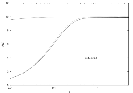
Figure 6: the hA amplitude $A(y,g)$ at $y=10$ for $\mu=1$, $\lambda=0.1$ (the lower curve) as compared to the pure fan prediction (the upper curve) and the asymptotic expression Eq. (120) (middle curve)

Figure 7: Same as Fig. 5 for $\mu=1$ and $\lambda=1/3$

Figure 8: The hA amplitude $A(y,g)$at $y=10$ for $\mu=-1$, $\lambda=0.1$ (the lower curve) as compared to the pure fan prediction (the upper curve)

References

- [1] A.H.Mueller, Nucl. Phys. B 437 (1995) 107.
- [2] D.Amati, L.Caneshi and R.Jengo, Nucl. Phys. B 101 (1975) 397.
- [3] V.Alessandrini, D.Amati and R.Jengo, Nucl. Phys. B 108 (1976) 425.
- [4] R.Jengo, Nucl. Phys. B 108 (1976) 447.
- [5] D.Amati, M.Le Bellac, G.Marchesini and M.Ciafaloni, Nucl. Phys. B 112 (1976) 107.
- [6] M.Ciafaloni, M. Le Bellac and G.C.Rossi, Nucl. Phys. B 130 (1977) 388.
- [7] M.Ciafaloni, Nucl. Phys. B 146 (1978) 427.
- [8] K.G.Boreskov, arXiv: hep-ph/0112325.
- [9] S.Bondarenko, L.Motyka, A.H.Mueller, A.I.Shoshi and B.-W.Xiao, hep-ph/0609213.
- [10] M. Kozlov and E. Levin, Nucl. Phys. A 779 (2006) 142.
- [11] M.Kozlov, E.Levin, V.Khachatryan and J.Miller, arXiv: hep-ph/0610084.
- [12] A.Schwimmer, Nucl. Phys. B 94 (1975) 445.
- [13] G.P.Salam, Nucl. Phys. b 461 (1996) 512.
- [14] Y. V. Kovchegov, Phys. Rev. D 72 (2005) 094009.
- [15] C. M. Bender and S. Boettcher, Phys. Rev. Lett. 80, 5243 (1998); C. M. Bender, D. C. Brody and H. F. Jones, Phys. Rev. Lett. 89, 270401 (2002) [Erratum-ibid. 92, 119902 (2004)].
- [16] A. Mostafazadeh, J. Math. Phys. 43, 3944 (2002); A. Mostafazadeh, J. Phys. A 38, 6557 (2005) [Erratum-ibid. A 38, 8185 (2005)].