Glueball Production via Gluonic Penguin B Decays

Abstract

We study glueball $G$ production in gluonic penguin decay $B\to X_{s}G$, using next-to-leading order $b\to sg^{*}$ gluonic penguin interaction and an effective coupling of a glueball to two gluons. The effective coupling allows us to study the decay rate of a glueball to two pseudoscalars in the framework of chiral perturbation theory. Identifying the $f_{0}(1710)$ to be a scalar glueball, we then determine the effective coupling strength with the branching ratio of $f_{0}(1710)\to K\overline{K}$. We find that the charm penguin to be important and obtain a sizable branching ratio for ${\rm Br}(B\to X_{s}G)$ in the range of $(0.7\sim 1.7)\times 10^{-4}$. Rare hadronic $B$ decay data from BABAR and Belle can provide important information about glueballs.

The existence of glueballs is a natural prediction of QCD. However, glueball state has not been confirmed experimentally. The prediction for the glueball masses is a difficult task. Theoretical calculations indicate that the lowest lying glueball state is a scalar with a mass in the range of 1.6 to 2 GeV. Recent quenched lattice calculations give a glueball mass $m_{G}$ equals $1710\pm 50\pm 80$ MeV lattice . These results support that the scalar meson $f_{0}(1710)$ to be a glueball. Phenomenologically, $f_{0}(1710)$ could be an impure glueball since it can be contaminated by possible mixings with the quark-antiquark states that have total isospin zero lee-weingarten ; burakovsky-page ; giacosa-etal ; close-zhao ; he-li-liu-zeng ; cheng-chua-liu ; fariborz . These mixing effects can be either small giacosa-etal ; close-zhao ; he-li-liu-zeng ; fariborz or large lee-weingarten ; burakovsky-page ; giacosa-etal ; cheng-chua-liu , depend largely on the mixing schemes one chose to do the fits and complicate the analysis. For simplicity, we will ignore these mixing effects and assume $f_{0}(1710)$ is indeed a glueball throughout this work.

Since the leading Fock space of a glueball $G$ is made up of two gluons, production of glueball is therefore most efficient at a gluonic rich environment like $J/\psi$ or $\Upsilon$ $\rightarrow(gg)\gamma\rightarrow G\gamma$ shifman ; jpsi . Direct glueball production is also possible at the $e^{+}e^{-}$ brodsky and hadron cky colliders. In this work, we point out another interesting mechanism to detect a glueball via the rare inclusive process $B\to X_{s}G$ decay. The leading contribution for this process is shown in Fig. [1], where the squared vertex refers to the gluonic penguin interaction and the round vertex stands for an effective coupling between a glueball and the gluons. The gluonic penguin $b\to sg^{*}$ has been studied extensively in the literature and was used in the context for inclusive decay $b\to sg\eta^{\prime}$ hou-tseng . The effective interaction for $b\to sg^{*}$ with next-to-leading QCD correction can be written as he-lin

$$\Gamma_{\mu a}=-{G_{F}\over\sqrt{2}}{g_{s}\over 4\pi^{2}}V_{ts}^{*}V_{tb}\bar{s}(p^{\prime})\,[\Delta F_{1}(q^{2}\gamma_{\mu}-q_{\mu}\not\!q)L-im_{b}F_{2}\sigma_{\mu\nu}q^{\nu}R]\,T^{a}\,b(p),$$ (1)

where $\Delta F_{1}=4\pi(C_{4}(q,\mu)+C_{6}(q,\mu))/\alpha_{s}(\mu)$ and $F_{2}=-2C_{8}(\mu)$ with $C_{i}(q,\mu)$ $(i=4,6,\,{\rm and}\,8$) the Wilson’s coefficients of the corresponding operators in the $\Delta B=1$ effective weak Hamiltonian, $q=p-p^{\prime}=k+k^{\prime}$, and $T^{a}$ is the generator for the color group. We will use the next-to-leading order numerical values of $\Delta F_{1}$ and $F_{2}$ he-lin . The top quark contribution gives $\Delta F^{\rm top}_{1}=-4.86$ and $F^{\rm top}_{2}=+0.288$ at $\mu=5$ GeV; whereas the charm quark contribution involves a $q^{2}$ dependence through $C_{4}^{\rm charm}(q,\mu)=C^{\rm charm}_{6}(q,\mu)=P^{\rm charm}_{s}(q,\mu)$ with

$$P^{\rm charm}_{s}(q,\mu) = {\alpha_{s}(\mu)\over 8\pi}C_{2}(\mu)\left({10\over 9}+Q(q,m_{c},\mu)\right)\;,$$ (2)

and

$$Q(q,m,\mu) = 4\int^{1}_{0}dx\,x\,(1-x)\ln\left[m^{2}-x(1-x)q^{2}\over\mu^{2}\right]\;\,$$

$$= \frac{2\left[3q^{2}\ln(m^{2}/\mu^{2})-12m^{2}-5q^{2}\right]}{9q^{2}}+\frac{4(2m^{2}+q^{2})\sqrt{4m^{2}-q^{2}}}{3\sqrt[3]{q^{2}}}{\rm arctan}\sqrt{\frac{q^{2}}{4m^{2}-q^{2}}}\;.$$

Here $m_{c}=$ 1.4 GeV is the charm quark mass and $C_{2}(\mu=5\,\mbox{GeV})=1.150$.

The following effective coupling between a scalar glueball and two gluons was advocated recently by Chanowitz chanowitz

$${\cal L}=f{\cal G}G^{a}_{\mu\nu}G^{a\mu\nu},$$ (4)

where ${\cal G}$ is the interpolating field for the glueball $G$, $G^{a}_{\mu\nu}$ is the gluon field strength, and $f$ is an unknown coupling constant. This form of effective coupling suggests that glueball couples to the QCD trace anomaly.

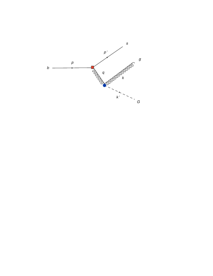
Figure 1: The leading diagram for $B\to X_{s}G$.

The interaction of a scalar glueball with light hadrons through the trace anomaly can be formulated systematically by using techniques of chiral Lagrangian, as was briefly mentioned in chm . The kinetic energy and the symmetry breaking mass terms for the light pseudoscalar mesons are given by donoghue

$${\cal L}_{\chi}={f^{2}_{\pi}\over 8}[{\rm Tr}(\partial^{\mu}\Sigma\partial_{\mu}\Sigma^{\dagger})+{\rm Tr}(\xi^{\dagger}\chi\xi^{\dagger}+\xi\chi\xi)],$$ (5)

where $f_{\pi}=132$ MeV being the pion decay constant, $\xi^{2}=\Sigma=\exp(2i\Pi/f_{\pi})$ with $\Pi$ the $SU(3)$ pseudoscalar octet meson,

$$\Pi=\left(\begin{array}[]{cccc}{1\over\sqrt{2}}\pi^{0}+{1\over\sqrt{6}}\eta&\pi^{+}&K^{+}\\ \pi^{-}&-{1\over\sqrt{2}}\pi^{0}+{1\over\sqrt{6}}\eta&K^{0}\\ K^{-}&{\overline{K}}^{0}&-{2\over\sqrt{6}}\eta\end{array}\right)\;,$$ (9)

and

$$\chi=2B_{0}\,{\rm diag}(\hat{m},\hat{m},m_{s})={\rm diag}(m^{2}_{\pi},m^{2}_{\pi},2m^{2}_{K}-m^{2}_{\pi})$$ (10)

with $B_{0}=2031$ MeV. Here we have neglected the isospin breaking effects due to small mass difference between the light $u$ and $d$ quarks and used $\hat{m}=m_{u}=m_{d}$. The QCD trace anomaly is well known and given by donoghue

$$\Theta^{\mu}_{\mu} = -\frac{b\alpha_{s}}{8\pi}G^{a}_{\mu\nu}G^{a\mu\nu}+\sum_{q}m_{q}\bar{q}q\;,$$ (11)

where $b=11-2n_{f}/3$ is the QCD one-loop beta function with $n_{f}=3$ being the number of light quarks. Treating the effective interaction (4) as a perturbation to the energy momentum stress tensor, one would then modify $\Theta^{\mu}_{\mu}$ to be

$$-\frac{b\alpha_{s}}{8\pi}G^{a}_{\mu\nu}G^{a\mu\nu}\left(1+f\frac{8\pi}{b\alpha_{s}}{\cal G}\right)+\sum_{q}\left(m_{q}+f_{q}{\cal G}\right)\bar{q}q\;,$$ (12)

where $f_{q}=f\alpha_{s}m_{q}(16\pi\sqrt{2}/3\beta)\ln\left[(1+\beta)/(1-\beta)\right]$ being the one-loop induced $Gq\bar{q}$ coupling chanowitz with $\beta=(1-4m^{2}_{q}/m_{G}^{2})^{1/2}$. Note that $f_{q}$ is proportional to $f$. The corresponding chiral Lagrangian is thus modified accordingly

$${\cal L}_{\chi} = {1\over 8}f^{2}_{\pi}\left(1+f{8\pi\over b\alpha_{s}}{\cal G}\right){\rm Tr}\left[\partial^{\mu}\Sigma\partial_{\mu}\Sigma^{\dagger}\right]$$ (13)

$$+ {1\over 8}f^{2}_{\pi}\,{\rm Tr}\left[\xi^{\dagger}(\chi+2B_{0}f_{\chi}{\cal G})\xi^{\dagger}+\xi(\chi+2B_{0}f_{\chi}{\cal G})\xi\right],$$

where $f_{\chi}={\rm diag}(f_{u},f_{d},f_{s})$. Using the above chiral Lagrangian, one can then calculate the decay rates for $G\rightarrow\pi^{+}\pi^{-},\pi^{0}\pi^{0},K^{+}K^{-},K^{0}{\overline{K}}^{0},\eta^{0}\eta^{0},$ and $\pi^{0}\eta^{0}$. Since $f_{0}(1710)$ is interpreted as the glueball, one can use the experimental branching ratio ${\rm Br}(f_{0}(1710)\rightarrow K{\overline{K}})=0.38^{+0.09}_{-0.19}$ and its total width $137\pm 8$ MeV pdg to be our input. Together with the decay rate formulas derived from the chiral Lagrangian (13) and a value of the strong coupling constant $\alpha_{s}=0.35$ extracted from the experimental data of $\tau$ decay, one can estimate the unknown coupling $f=0.07^{+0.009}_{-0.018}$ ${\rm GeV}^{-1}$.

In our estimation of $f$ given above, we have extrapolated low energy theorems to the glueball mass scale. One might overestimate the hadronic matrix elements in due course. This implies that the extracted value of $f$ would be too small.

Decay $G\to K\overline{K}$ has also been obtained using perturbative QCD calculations chm . This approach can also give some estimate of the amplitude. The problem facing this approach is that the energy scale may not be high enough to have the perturbative QCD contribution to dominate. Using the asymptotic light-cone wave functions, we find that for a given branching ratio for $G\to K\overline{K}$ decay, the resulting $f$ would be about 20 times larger than the value obtained above using the chiral approach. Incidentally, the value of $f$ derived from the chiral Lagrangian is within a factor of 2 compared with the value estimated just by using the free quark decay rate of $G\rightarrow s\bar{s}$ cky . In our later calculations, we will use the conservative value $f=0.07^{+0.009}_{-0.018}$ ${\rm GeV}^{-1}$ determined using the chiral Lagrangian given in Eq.(13). This will give the most conservative estimate for the branching ratio since the chiral approach gives the smallest $f$.

With the two effective couplings given in Eqs.(1) and (4), the following decay rate for $b\rightarrow sgG$ (Fig.(1)) can be obtained readily

$$\Gamma_{b\rightarrow sgG} = \left({N_{c}^{2}-1\over 4N_{c}}\right){G_{F}^{2}m_{b}^{5}|V^{*}_{ts}V_{tb}|^{2}\over 2^{5}\pi^{3}}\left({g_{s}\over 4\pi^{2}}\right)^{2}(m_{b}f)^{2}$$ (14)

$$\times\int_{0}^{(1-\sqrt{x^{\prime}})^{2}}dx\int_{y_{-}}^{y_{+}}dy\left\{|\Delta F_{1}|^{2}c_{0}+{\rm\bf Re}(\Delta F_{1}F^{*}_{2}){c_{1}\over y}+|F_{2}|^{2}{c_{2}\over y^{2}}\right\}\;,$$

with

$$y_{\pm}={1\over 2}\left[(1-x+x^{\prime})\pm\sqrt{(1-x+x^{\prime})^{2}-4x^{\prime}}\right]\;.$$ (15)

In Eq.(14), $N_{c}$ is the number of color and $c_{0,1,2}$ are given by

$$c_{0} = \frac{1}{2}[-2x^{2}y+(1-y)(y-x^{\prime})(2x+y-x^{\prime})]\;,$$

$$c_{1} = (1-y)(y-x^{\prime})^{2}\;,$$

$$c_{2} = \frac{1}{2}[2x^{2}y^{2}-(1-y)(y-x^{\prime})(2xy-y+x^{\prime})]\;,$$ (16)

with $x=(p^{\prime}+k)^{2}/m^{2}_{b}$, $y=(k+k^{\prime})^{2}/m^{2}_{b}$, and $x^{\prime}=m^{2}_{G}/m^{2}_{b}$.

Using the value of $f$ determined above from the chiral Lagrangian, we find the branching ratio for $b\to sgG$ to be $4.5\times 10^{-5}(f\cdot\mbox{GeV}/0.07)^{2}$ with just the leading top penguin contribution to $\Delta F_{1}$ is taken into account. The correction from the charm penguin is nevertheless substantial and should not be neglected. Inclusion of both top and charm penguins gives rise to an enhancement about a factor of 3 in the branching ratio ${\rm Br}(b\to sgG)\approx 1.3\times 10^{-4}(f\cdot\mbox{GeV}/0.07)^{2}$. Since $f_{0}(1710)$ has a large branching ratio into $K\overline{K}$, the signal of scalar glueball can be identified by looking at the secondary $K\overline{K}$ invariant mass. The recoil mass spectrum of $X_{s}$ can also be used to extract information. The distribution of $d{\rm Br}(b\to sgG)/dM_{X_{s}}$ as a function of the recoil mass of $X_{s}$ is plotted in Fig.(2).

Figure 2: $d{\rm Br}(B\to X_{s}G)/dM_{X_{s}}$ in unit of $10^{-5}$. In the figure the $b$ quark mass $m_{b}$ is taken to be 4.248 GeV, $\alpha_{s}=0.21$ at the $b$ quark scale, $\tau_{B}=1.674\times 10^{-12}$ s, and $f=0.07$ GeV^-1.

Analogously one can also study inclusive $B$ decays into a pseudoscalar glueball $\tilde{G}$, whose leading effective coupling to the gluon can be parameterized as cornwall-soni ,

$${\cal L}=\tilde{f}\tilde{\cal G}\tilde{G}^{a}_{\mu\nu}G^{a\mu\nu}\;\;\;\;{\rm with}\;\;\;\;\tilde{G}^{a}_{\mu\nu}={1\over 2}\epsilon_{\mu\nu\alpha\beta}G^{a\alpha\beta}\;,$$ (17)

and $\tilde{\cal G}$ denoting the interpolating field for the pseudoscalar glueball. The decay rate for this case can be deduced from the scalar glueball one by replacing the coupling $f$ with $\tilde{f}$ and the mass $m_{G}$ with the pseudoscalar glueball mass $m_{\tilde{G}}$ in Eq.(14). This also reproduces previous result obtained in Ref.hou-tseng for a similar process $b\rightarrow sg\eta^{\prime}$. We therefore expect similar distribution and branching ratio for the pseudoscalar glueball production from the $B$ decay as in the scalar case that we have studied in this work.

Recently, BES has observed an enhanced decay in $J/\psi\to\gamma\eta^{\prime}\pi\pi$ with a peak around the invariant mass of $\eta^{\prime}\pi\pi$ at 1835 MeV bes2 . Proposal has been made to interpret this state $X(1835)$ to be due to a pseudoscalar glueball hhh . Taking $X(1835)$ to be a pseudoscalar glueball, we would obtain a branching ratio of $3.7\times 10^{-5}(\tilde{f}\cdot\mbox{GeV}/0.07)^{2}$ with top penguin contribution only, and is enhanced to $1.1\times 10^{-4}(\tilde{f}\cdot\mbox{GeV}/0.07)^{2}$ if charm penguin is also included. If the coupling $\tilde{f}$ is of the same order of magnitude as $f$, the branching ratio for $B\to X_{s}\tilde{G}$ is also sizable. Pseudoscalar glueball may also be discovered in rare $B$ decays. Since a pseudoscalar glueball cannot decay into two pseudoscalar mesons, the identification of a pseudoscalar glueball necessitates the study of the three-body system $\eta^{\prime}\pi\pi$. This makes the analysis more difficult compared with the case of a scalar glueball.

To conclude, we have studied inclusive production of a scalar glueball in rare $B$ decay through the gluonic penguin and an effective glueball-gluon interaction. The branching ratio is found to be of the order $10^{-4}$. $B$ decays into a pseudoscalar glueball through gluonic penguin is also expected to be sizable. Note that we have used a conservative estimate of $f$. Observation of $B\to X_{s}f_{0}(1710)$ at a branching ratio of order $10^{-4}$ or larger will provide an strong indication that $f_{0}(1710)$ is mainly a scalar glueball. With more than 600 millions of $B\overline{B}$ accumulated at Belle and more than 300 millions at BABAR, test of ${\rm Br}(b\to sgG)$ at the level of $10^{-4}$ is quite feasible. We strongly urge our experimental colleagues to carry out such an analysis.

References

(1)
Y. Chen, A. Alexandru, S. J. Dong, T. Draper, Horv th, F. X. Lee, K. F. Liu, N. Mathur, C. Morningstar,
M. Peardon, S. Tamhankar, B. L. Yang, and J. B. Zhang, Phys. Rev. D 73, 014516 (2006)
[arXiv:hep-lat/0510074].
(2)
W. Lee and D. Weingarten, Phys. Rev. D 61, 014015 (1999); [arXiv:hep-lat/9805029].
(3)
L. Burakovsky and P. R. Page, Phys. Rev. D 59, 014022 (1998).
(4)
F. Giacosa, Th. Gutsche, V. E. Lyubovitskij, and A. Faessler, Phys. Rev. D 72, 094006 (2005).
(5)
F. E. Close and Q. Zhao, Phys. Rev. D 71, 094022 (2005).
(6)X. G. He, X. Q. Li, X. Liu, and X. Q. Zeng, Phys. Rev. D 73, 051502 (2006);
ibid. D 73, 114026 (2006).
(7)A. H. Fariborz, Phys. Rev. D 74 054030 (2006)
[arXiv:hep-ph/0607105].
(8)H. Y. Cheng, C. K. Chua, and K. F. Liu,
arXiv:hep-ph/0607206.
(9) V. A. Novikov, M. A. Shifman, A. I. Vainshtein, and
V. I. Zakharov, Nucl. Phys. B165, 67 (1980).
(11) S. Brodsky, A. S. Goldhaber, and J. Lee, Phys.
Rev. Lett. 91, 112001 (2003).
(12)
K.m. Cheung, W. Y. Keung, and T. C. Yuan, in preparation.
(13)
D. Atwood and A. Soni, Phys. Lett. B 405, 150 (1997); W.
S. Hou and B. Tseng, Phys. Rev. Lett. 80, 434 (1998).
(14)X. G. He and G. L. Lin, Phys. Lett. B 454, 123 (1999). In Eq.(4) of this paper,
should be replaced by .
(15) M. S. Chanowitz,
Phys. Rev. Lett. 95, 172001 (2005) [arXiv:hep-ph/0506125].
(16)
K. T. Chao, X. G. He, and J. P. Ma,
arXiv:hep-ph/0512327.
(17)
For an introductory exposition of chiral Lagrangian, we refer to the textbook by
J. F. Donoghue, E. Golowich, and B. R. Holstein, Dynamics of the Standard Model,
Cambridge University Press (1992).
(18) W.-M. Yao et al., Particle Data Group, J. Phys. G33, 1 (2006).
(19)
J. M. Cornwall and A. Soni, Phys. Rev. D 32, 764 (1985); ibid. D 29, 1424 (1984).
(20) M. Ablikim et al., (BES Collaboration), Phys. Rev.
Lett. 95, 262001(2005).
(21) X.-G. He, Xue-Qian Li, Xiang Liu, and J. P. Ma, arXiv:hep-ph/0509140.