String compactification, QCD axion and axion-photon-photon coupling

Abstract:

It is pointed out that there exist a few problems to be overcome toward an observable sub-eV QCD axion in superstring compactification. We give a general expression for the axion decay constant. For a large domain wall number $N_{DW}$, the axion decay constant can be substantially lowered from a generic value of a scalar singlet VEV. The Yukawa coupling structure in the recent ${\bf Z}_{12-I}$ model is studied completely, including the needed nonrenormalizable terms toward realistic quark and lepton masses. In this model we find an approximate global symmetry and vacuum so that a QCD axion results but its decay constant is at the GUT scale. The axion-photon-photon coupling is calculated for a realistic vacuum satisfying the quark and lepton mass matrix conditions. It is the first time calculation of $c_{a\gamma\gamma}$ in realistic string compactifications: $c_{a\gamma\gamma}$$=\frac{5}{3}-1.93\simeq-0.26$.

1 Introduction and Summary on Superstring Axions

The strong CP problem is, $``$Why is the QCD vacuum angle $\bar{\theta}_{\rm QCD}$ so small at $|\bar{\theta}_{\rm QCD}|<10^{-9}$?” Otherwise, strong QCD interactions violate the CP symmetry and then neutron will develop an electric dipole moment of order $10^{-3}|\bar{\theta}_{\rm QCD}|\times$(charge radius of neutron), and the present upper bound on the neutron electric dipole moment $d_{n}<0.63\times 10^{-25}$e cm [2] restricts $|\bar{\theta}_{\rm QCD}|<10^{-9}$. There are a few solutions of the strong CP problem [3]: (i) Set $\bar{\theta}_{\rm QCD}=0$ at tree level and guarantee that loop effects are sufficiently small, (ii) $m_{u}=0$ method, and (iii) the Peccei-Quinn (PQ) mechanism. Axion solutions which we discuss in this paper belong to Case (iii). The PQ mechanism [4] introduces an anomalous (in the QCD gluon fields) global U(1)_PQ symmetry. This must be an axial symmetry. Since quarks are massive, the global U(1)_PQ symmetry must be spontaneously broken, generating a Goldstone boson called axion [5]. Currently, the phenomenologically allowable QCD axion is a very light axion [6]. A probable initial condition of the axion decay constant allows the window, $10^{10}\ {\rm GeV}\leq F_{a}\leq 10^{12}$ GeV. But, with the anthropic principle applied, the upper bound can be further open [7].

Axion models in field theory are artificial in the sense that the U(1)_PQ symmetry is given for the sake of the PQ mechanism only. It is desirable if a consistent theory with an ultraviolet completion gives a natural candidate for axion. In this regards, we consider string models. If a string theory predicts a phenomenologically allowable axion, this may be a key prediction of string theory. This is welcome in view of the scarcity of direct verifiable methods of $`$string’ nature. In fact, one attractive feature of string theory is the natural appearance of axions from the antisymmetric tensor field $B_{MN}$. These superstring axions are split into two categories: one is the compactification scheme independent one called model-independent axion (MI axion) $B_{\mu\nu}$ [8] and the other is the compactification dependent one called model-dependent axion (MD axion) $B_{ij}$ [9]. However, these superstring axions are known to have some problems. Derived from string theory, decay constants of these axions are expected to be near the string scale $\sim 10^{16}$ GeV [10], outside the aforementioned axion window. For MD axions, it is further known that the shift symmetries of MD axions are broken at high energy scales [11] so that they cannot be used as axions for rolling the vacuum angles to zero [3]. However, one should not forget that such superpotential of MD axions is a model-dependent statement [12]. Recently, there has been attempts to lower the decay constants in string models or in higher dimensional models [13, 14, 15, 16, 17]. One approach is a large volume compactification to lower the fundamental scale [13]. Another approach is using the warped geometry to lower the scale. In heterotic flux compactification, MD axions can be localized at a vanishing cycle which is warped due to the flux so that we may have a small axion decay constant [15]. Similar setup has been discussed in a higher-dimensional model[16]. In other contexts, an axion in the Kachru-Kallosh-Linde-Trivedi setup has also been discussed in [17].

In this paper, we restrict the discussion on superstring axions to heterotic string only, but the generic problem of axion mixing is present in any superstring axion models. For the MI axion, the decay constant is near the scale $\sim 10^{16}$ GeV [10]. Some string compactifications such as the simple compactifications of Refs. [18, 19] do not lead to an anomalous U(1), in which case the MI axion is harmful [10]. Later, it was found that some string compactifications lead to an anomalous U(1) gauge symmetry [20]. This anomalous symmetry can be gauged owing to the Green-Schwarz mechanism by which the antisymmetric tensor field $B_{\mu\nu}$ transforms nonlinearly under the U(1) symmetry so as to cancel the anomaly [20]. This anomalous U(1) gauge symmetry is a subgroup of SO(32) or of E${}_{8}\times$E${}_{8}^{\prime}$. The Green-Schwarz term [22] makes it possible for this anomalous U(1) gauge boson to absorb the MI axion and become massive. Below this gauge boson mass scale $\sim 10^{16}$ GeV, there results a global symmetry U(1)_an. This is a kind of ’t Hooft mechanism [23]. Under this circumstance, if some scalar field carrying U(1)_an charges develop VEVs around $\sim 10^{11}$ GeV, then we obtain a harmless very light axion by the PQ mechanism [4]. However, for this U(1)_an, the story is not that simple. Most light fields carry nonvanishing U(1)_an charges, and if one is forced to give GUT scale VEVs to those singlets for successful Yukawa coupling textures, then the U(1)_an breaking scale must be the GUT scale and the resulting axion is again harmful. The QCD axion with this U(1)_an has been extensively studied without any hidden sector confining force in [24], where the Yukawa coupling textures were not used. Moreover, this model is phenomenologically unsatisfactory since $\sin^{2}\theta_{W}\ll\frac{3}{8}$.

Most string compactifications need another confining force in the hidden sector for the purpose of introducing supersymmetry breaking. Then, we need an additional global symmetry to settle both QCD and hidden sector $\theta$s. As mentioned above, only the U(1)_an, related to the MI axion, is a good one to consider below the string scale. Except this U(1)_an, there is no global continuous symmetry resulting from string theory. For an additional global symmetry, we are only at a disposal of approximate global symmetries from string compactification. It is better for this approximate global symmetry to be broken by a sufficiently high dimensional operators in the superpotential so that the symmetry breaking superpotential is negligible compared to the axion potential derived from anomalies. This idea was examined in a SUGRA field theory model with a discrete ${\bf Z}_{3}\times{\bf Z}_{3}$ symmetry [25]. But it has not been studied in string compactifications. A discrete symmetry is a good guideline to make approximate symmetry violating terms appear at higher orders. If PQ symmetry breaking scales are around the intermediate scale, it has been known that the PQ symmetry breaking superpotential must be forbidden up to $D=9$ terms [26]. But this statement is an oversimplified one because higher order terms can involve some scalar fields developing small VEVs or even not developing any VEV. So, the PQ symmetry violating terms in the superpotential must be checked in model-by-model bases. Note that for the terms breaking the global symmetry to appear at a sufficiently higher order, we need a large $N$, presumably $N=12$, in the ${\bf Z}_{N}$ orbifold compactifications.

By the way, the MSSMs from superstring need Yukawa couplings beyond cubic terms [27, 28]. So far, there has not appeared any model where only cubic terms are sufficient to give all the needed Yukawa couplings. So it is not unreasonable to require that for realistic quark and lepton masses superstring models need nonrenormalizable terms beyond cubic terms.

Thus, to realize a QCD axion in string compactifications, we must satisfy the following conditions:

• One must work in a phenomenologically successful string derived model.

• One needs an additional confining group beyond QCD, and an approximate global symmetry must be introduced. The MD axions cannot be used since the world sheet instanton effects violate the shift symmetries of the MD axions.

• The Yukawa coupling structure must be studied carefully to derive the approximate global symmetry.

• With two axions, the axion mixing effect must be clarified.

So far, there has not appeared any literature satisfying all the above conditions. In this paper, we try to explore the possibility of satisfying all these conditions in the recently proposed string MSSM [27]. We find a vacuum satisfying all of these conditions, but the QCD axion decay constant falls in the GUT scale region.

We emphasize the importance of the last condition which has been overlooked in many superstring axion models. It is studied in Refs. [29, 15]. There is the cross theorem on axion potential heights and decay constants. It is for the case of two $\theta$s with a complete mixing of two axions by the higher potential that the smaller decay constant corresponds to the higher height of the axion potentials and the larger decay constant corresponds to the lower height of the axion potentials. It is shown for the case of two axions with the MI axion and the MD axion corresponding to the breathing mode moduli [30] where the couplings are $\sim a_{1}(F\tilde{F}+F^{\prime}\tilde{F}^{\prime})+a_{2}(F\tilde{F}-F^{\prime}\tilde{F}^{\prime})$. In fact, the axion mixing occurs when both axions couple to the anomaly which give rise to the higher potential from instanton. In the example of [30], two anomalies couple to both axions and hence the condition for the theorem is satisfied. In such cases, if the hidden sector axion potential is higher than the QCD axion potential (as one might guess), then the decay constant of the QCD axion is the GUT scale. If we realize that the decay constant of the QCD axion falls around $\sim 10^{11}$ GeV, then it will be observable by axion detection experiments like the CAST of CERN [31].

After solving the strong CP problem, we can consider a related, the so-called $\mu$ problem [32], derivable from the global symmetries of the MSSM. The common origin of a very light axion scale and supergravity scale was pointed out early [33]. Phenomenologically, the strength of the $\mu$ parameter in $-\mu H_{u}H_{d}$ is required to be at the electroweak scale. The first $\mu$ problem is why it is forbidden at the Planck scale. The second $\mu$ problem is why it is of order the electroweak scale. There have been suggestions that if it is forbidden at the GUT scale, it is expected to be generated at the electroweak scale in supergravity models [34] and in string models [35]. However, these solutions need some symmetry anyway from the Yukawa coupling structure to forbid it at scales below the GUT scale [36]. If many singlet VEVs are required at the GUT scale, then forbidding just $H_{u}H_{d}$ in the renormalizable superpotential as done in [35] is not enough to exclude the $\mu$ term at the GUT scale.

In this paper, in addition we try to calculate the axion-photon-photon coupling $c_{a\gamma\gamma}$ in a realistic superstring model. For the MI axion, a mechanism to find out the global U(1)_an was explicitly given before [24] but a calculation of $c_{a\gamma\gamma}$ in that model has not been meaningful because the model is not realistic due to $\sin^{2}\theta_{W}\ll\frac{3}{8}$ and there is no additional confining force for supersymmetry breaking. Now we obtained a realistic superstring standard model in a ${\bf Z}_{12-I}$ construction [27] and here we can calculate $c_{a\gamma\gamma}$ if there exists a QCD axion.

We may introduce two scales (at $M_{\rm GUT}$ and $10^{11}$ GeV) for breaking U(1)_an and an approximate global symmetry U(1)_glA. The resulting approximate global current must be anomalous in the gluon fields and/or hidden confining gauge fields. The axion mixing is studied with the hidden sector axion potential.

In this paper, we pick up an approximate global symmetry U(1)_glA in addition to U(1)_an. We use a computer program which is based on the Gauss elimination algorithm to study all possible U(1) symmetries from any order of Yukawa couplings. A complete analysis has been done for all Yukawa couplings up to $D=9$ superpotential terms. Unfortunately, we could not realize the QCD axion with $F_{a}\sim 10^{11}$ GeV but at the GUT scale. The axion energy crisis may be resolved by the anthropic principle [7]. We calculate the phenomenologically important axion-photon-photon coupling constant $c_{a\gamma\gamma}$, i.e. $\tilde{c}_{a\gamma\gamma}=\frac{5}{3}$ or $c_{a\gamma\gamma}$$\simeq-0.26$. This is the first calculation of $c_{a\gamma\gamma}$ from a realistic string compactification.

This paper is organized as follows. In Sec. 2, we summarize briefly axion physics related to the calculation of the axion decay constant. This involves a discussion on the domain wall number of discrete vacua. In Sec. 3, we succinctly present the recent ${\bf Z}_{12-I}$ orbifold model [27] toward a computer input for the matter fields. In Sec. 4, we summarize the Yukawa coupling structure and find the anomalous U(1)_an symmetry from E${}_{8}\times$E${}_{8}^{\prime}$ and an approximate anomalous global symmetry U(1)_glA so that two $\theta$s can be settled to zero via the PQ mechanism. In Sec. 5, we calculate the axion-photon-photon coupling by calculating anomalies. It is compared to the recent CAST experiment bound [31]. Sec. 6 is a conclusion.

2 Axion, Domain Walls and Axion Decay Constant

The QCD axion $a$ is defined to be a pseudoscalar particle coupling to the gluon anomaly,

$$\frac{a}{32\pi^{2}F_{a}}G_{\mu\nu}\tilde{G}^{\mu\nu}\equiv\frac{a}{F_{a}}\{G\tilde{G}\}$$ (1)

where $\tilde{G}^{\mu\nu}$ is the dual of $G^{\mu\nu}$, the gluon kinetic term is $(1/4g_{c}^{2})G_{\mu\nu}G^{\mu\nu}$ and $F_{a}$ is the axion decay constant. It is assumed that there exists the canonical kinetic energy term of $a$, i.e. $\frac{1}{2}\partial_{\mu}a\partial^{\mu}a$, and there is no potential for the axion except that derivable from Eq. (1). Then, the minimum of the axion potential is at $\langle a\rangle=0$ [4, 37] which solves the strong CP problem cosmologically in the present universe [38]. We do not repeat the explanation of the solution of strong CP problem using the axion in this section. For a complete review, refer to [3]. Here, we discuss some subtlety of determining the axion decay constant due to the remaining discrete group after U(1)_PQ breakdown.

Because of the quantization of the integral of $G\tilde{G}$, the axion potential is periodic with the periodicity $2\pi F_{a}$. In this form Eq. (1), the fundamental region of the axion vacua is $[0,2\pi F_{a}]$, because $\bar{\theta}=[0,2\pi]$. Namely, starting from the vacuum $\langle a\rangle=0$, the next vacuum occurs by shifting $\langle a\rangle\to\langle a\rangle+2\pi F_{a}$. But the vacuum at $\langle a\rangle=2\pi F_{a}$ may not be the same vacuum as the $\langle a\rangle=0$ vacuum, but returns to the $\langle a\rangle=0$ vacuum only after the shift $a\to a+2\pi N_{DW}F_{a}$. Then there are degenerate vacua whose number is called the domain wall number $N_{DW}$ [39]. The axion embedded in some fields may not return to its original value when one shifts $a\to a+2\pi F_{a}$, which is the reason for the appearance of degenerate vacua. There is another degeneracy from the scalar field space. Suppose, the axion $a$ embedded in the phase of a scalar field as $\phi=[{(v+\rho)/\sqrt{2}}]e^{ia/v}$ where $\phi$ carries $N$ units of PQ charge. The field $\phi$ returns to its original value by shifting $a\to a+2\pi v$. But the phase factor becomes identity for $N$ distinct points of $0\leq a<2\pi v$. This is related to the domain wall number calculation. If we define the PQ charge $Q$ such that $\phi$ carries one unit of $Q$ and the anomaly calculation leads to $\partial_{\mu}J^{\mu}_{\rm PQ}=n\{G\tilde{G}\}$, the phase $a$ couples to the anomaly as $\frac{a}{v}n\{G\tilde{G}\}$. Since $\phi$ is defined such that it comes to the original value by the PQ transformation or the shift of $a$ by $a\to a+2\pi v$, viz. $Q=1$, this interaction defines $F_{a}=v/n$. Here, the domain wall number is $N_{DW}=n$.

On the other hand, if we are required (by the PQ charges of the other fields) to define the PQ charge of $\phi$ as $\Gamma$ which is a positive integer greater than 1, then $\partial_{\mu}J^{\mu}_{\rm PQ}=\Gamma n\{G\tilde{G}\}$, and we expect the axion decay constant $F_{a}=v/n\Gamma$. But the domain wall number defined from vacuum structure is a topological one and still we should obtain $N_{DW}=n$. This situation is illustrated for $N_{1}=n\Gamma=4$ and $N_{2}=\Gamma=2$, i.e. with $n=2$ in Fig. 1.

Figure 1: Illustration of degenerate vacua for $N_{1}=4,N_{2}=2$. Bullets and circles correspond to minima of the axion potential. (a) $N_{DW}$ is two, the vacua connected by solid and dashed lines. (b) The fundamental length (the arrow) in the fundamental region corresponds to the decay constant which is $F_{a}=V/N_{DW}\Gamma$.

Certainly, the minima of the axion potential has two distinct sets in Fig. 1(a), the set of bullets and the set of circles, represented by the connections with solid and dashed lines, respectively. These two sets agree with our original domain wall number, $N_{DW}=n=2$. This domain wall number is obtained from $N_{1}$ (the coefficient of anomaly) by dividing it with the greatest common divisor of $N_{1}$ and $N_{2}$. In Fig. 1(b), we show how our $F_{a}$ is related to the original VEV.

Having specified the domain wall number, it is important to pick up the properly normalized axion field toward calculating the axion decay constant. Consider two fields $\phi_{1}$ and $\phi_{2}$. In the unitary gauge, we can express the Goldstone bosons in the phases of $\phi_{1}$ and $\phi_{2}$ as

$$\phi_{1}=\frac{V_{1}+\rho_{1}}{\sqrt{2}}e^{iA_{1}/V_{1}},\quad\phi_{2}=\frac{V_{2}+\rho_{2}}{\sqrt{2}}e^{iA_{2}/V_{2}}$$ (2)

whose PQ charges are $\Gamma_{1}$ and $\Gamma_{2}$, respectively. Now we can restrict the phase fields $A_{1}=[0,\frac{1}{\Gamma_{1}}V_{1}]$ and $A_{2}=[0,\frac{1}{\Gamma_{2}}V_{2}]$. If we are sitting in one domain, say on the solid line (or on the dashed line) of Fig. 1 for reinterpreting the figure with $A_{1}$ and $A_{2}$ directions with $\Gamma_{1}=4$ and $\Gamma_{2}=2$, $A_{1}$ and $A_{2}$ completely define the allowed field space in that domain. Thus, we can represent the fields in one domain as

$$\phi_{1}=\frac{V_{1}+\rho_{1}}{\sqrt{2}}e^{iA_{1}/(V_{1}/4)},\quad A_{1}=[0,\frac{V_{1}}{2}]$$ (3)

$$\phi_{2}=\frac{V_{2}+\rho_{1}}{\sqrt{2}}e^{iA_{2}/(V_{2}/2)},\quad A_{2}=[0,\frac{V_{2}}{2}].$$ (4)

The relevant VEV for axion is $\sqrt{4^{2}V_{1}^{2}+2^{2}V_{2}^{2}}$. The axion direction in terms of $`A$’s is $\theta_{A}=\frac{4A_{1}+2A_{2}}{\sqrt{4^{2}V_{1}^{2}+2^{2}V_{2}^{2}}}$. Suppose that the gluon anomaly were just one unit of $\{G\tilde{G}\}$. Then, the axion coupling is given by

$$\frac{4A_{1}+2A_{2}}{\sqrt{4^{2}V_{1}^{2}+2^{2}V_{2}^{2}}}\{G\tilde{G}\}$$ (5)

With the shifts of $A_{1}\to A_{1}+2\pi V_{1}$ and $A_{2}\to A_{2}+2\pi V_{2}$, viz. Fig. 1, the field space ends at the other domain, i.e. $A_{i}$ shifted such that $\theta$ changed by $4\pi$. So to maintain the fields in the same domain with $\theta=[0,2\pi)$, we use $A_{i}=2a_{i}$ such that $a_{i}\to a_{i}+2\pi F_{i}$. Thus, we have $F_{i}=V_{i}/2$. Thus, the coupling (5) can be rewritten as

$$\frac{2(4a_{1}+2a_{2})}{\sqrt{4^{2}V_{1}^{2}+2^{2}V_{2}^{2}}}\{G\tilde{G}\}=2({\rm dimensionless\ axion\ component\ in\ the\ phase})\{G\tilde{G}\}$$ (6)

where the overall factor 2 appears as the greatest common divisor (GCD) of $\Gamma_{1}$ and $\Gamma_{2}$. For one field VEV dominating the other, e.g. the DFSZ model with a large singlet VEV $\langle s^{0}\rangle$ and a small doublet VEV, the dimensionless axion component is in fact $a_{1}/\langle s^{0}\rangle$ and the axion decay constant is $F_{a}=\langle s^{0}\rangle/2$.

If we consider the domain wall number from the gluon anomaly, that should be considered also and an appropriate factor must be multiplied to Eq. (6). If the anomaly coefficient $N(\rm anom.)$ from the gluon anomaly and $N({\rm phase})$ from a multitude of phases are relatively prime, then the domain wall number is simply $N({\rm anom.})$. But if they are not relatively prime, we must divide it by the greatest common divisor of $N({\rm anom.})$ and $N({\rm phase})$. Therefore, a general expression for the axion coupling can be written as

$$\frac{N_{DW}\cdot D_{\rm GCD}({\rm phase})}{V_{\rm max}}\ a\{G\tilde{G}\}$$ (7)

where $D_{\rm GCD}$ is the greatest common divisor of PQ charges of the relevant VEV-carrying fields, and the topological number $N_{DW}$ is calculated as in Fig. 1(a) from the coefficient of the anomaly and the phase degeneracy, i.e. $N_{DW}=N({\rm anom.})/D_{\rm GCD}(N({\rm anom.}),N({\rm phase}))$. The normalized axion field is defined as

$$\frac{a}{V_{\rm max}}\equiv\frac{\sum_{i}\Gamma_{i}a_{i}}{\sqrt{\sum\Gamma_{i}^{2}V_{i}^{2}}}$$ (8)

where $\Gamma_{i}$ is the U(1)_PQ charge of $s_{i}$, $V_{i}$ is the VEV of scalar field $\langle s_{i}\rangle$, and $V_{\rm max}$ is a typical scale of VEVs breaking the global symmetry. In many cases it is the maximum value among $\langle s_{i}\rangle$. For example, for the case $V_{\rm max}\gg V_{i}(i\neq{\rm max})$ and also for $V_{\rm max}=V_{i}({\rm for\ any\ }i)$. Then the axion decay constant is

$$F_{a}=\frac{V_{\rm max}}{N_{DW}\cdot D_{\rm GCD}}\ .$$ (9)

Note that if $N_{DW}\cdot D_{\rm GCD}$ were large, then $F_{a}$ can be lowered significantly compared to the PQ symmetry breaking scale.

The discussion of this section will be used in Sec. 5 in estimating the decay constant of the QCD axion from superstring.

3 ${\bf Z}_{12-I}$ Orbifold Model

In this section, we briefly summarize the key points of a realistic string-derived minimal supersymmetric standard model (MSSM) from a ${\bf Z}_{12-I}$ orbifold compactification [27]. Here, the low energy effective theory contains the MSSM. We discuss vacuum configuration of the MSSM singlets for realistic low energy phenomenology, especially toward the absence of exotic matter spectra and general formulae for realistic Yukawa couplings. These formulae are used in the program to generate all Yukawa couplings. We pick up the anomalous gauged U(1), U(1)_an, and approximate global U(1)s which appear in general in lower dimensional superpotential terms. For gauged U(1)s, the gauge U(1) directions can be assigned in the E${}_{8}\times$E${}_{8}^{\prime}$ group space but for the approximate global U(1)s it cannot be represented in that way. The only method for approximate global U(1)s is to list the U(1) charges of the matter fields.

3.1 Flipped SU(5) matter spectrum and Yukawa couplings

In the orbifold compactification in heterotic string theories, the action of twisting is represented as a shift vecdtor $V^{I}(I=1,2,\dots,16)$ and Wilson Lines $a_{i}^{I}(i=1,2,\dots,6;I=1,2,\dots,16)$. In the ${\bf Z}_{12-I}$ orbifold model discussed in [27], we choose SU(3)$\times$SO(9) lattice for toroidal compactification and

$$V=\textstyle\left(\frac{1}{4}~{}\frac{1}{4}~{}\frac{1}{4}~{}\frac{1}{4}~{}\frac{1}{4}~{}\frac{5}{12}~{}\frac{6}{12}~{}0~{}\right)\left(\frac{2}{12}~{}\frac{2}{12}~{}0~{}0~{}0~{}0~{}0~{}0\right)$$ (10)

$$a_{3}=a_{4}=\textstyle\left(0^{5}~{}0~{}\frac{-1}{3}~{}\frac{1}{3}~{}\right)\left(0~{}0~{}\frac{2}{3}~{}0^{5}\right)$$ (11)

$$a_{1}=a_{2}=a_{5}=a_{6}=0.$$

Then, below the compactification scale one obtains the following unbroken gauge group

$$[SU(5)\times U(1)_{X}\times U(1)^{3}]\times[SU(2)\times SO(10)\times U(1)^{2}]^{\prime}.$$ (12)

The spectra for the unbroken subgroup SU(5)$\times$U(1)_X is in fact the flipped SU(5) model [27]. The matter representations under the nonabelian gauge groups SU(5), SU(2)^′ and SO(10)^′ are simply determined by embedding the momenta $P$ of E${}_{8}\times$E${}_{8}^{\prime}$ group space into the weight space of the corresponding subgroup. The U(1) charges for matter fields are determined by

$$q_{i}=Z_{i}\cdot(P+k(V+m_{f}a_{3})),$$ (13)

where $i=X,1,2,3,4,5$ denotes each U(1) gauge group and $k$ corresponds to the orbifold twist number of $k$-th twisted sector and $m_{f}$ is the Wilson line twist number applicable only to the second two-torus, viz. (11). $Z_{i}$ are the following E${}_{8}\times$E${}_{8}^{\prime}$ weights

$$Z_{1}=(2,2,2,2,2;0^{3})(0^{8})^{\prime}$$ (14)

$$Z_{2}=(0^{5};1,0,0)(0^{8})^{\prime}$$ (15)

$$Z_{3}=(0^{5};0,1,0)(0^{8})^{\prime}$$ (16)

$$Z_{4}=(0^{5};0,0,1)(0^{8})^{\prime}$$ (17)

$$Z_{5}=(0^{8})(1,1;0;0^{5})^{\prime}$$ (18)

$$Z_{6}=(0^{8})(0,0;1;0^{5})^{\prime}.$$ (19)

We will rearrange these U(1)s when we consider the gauge anomalies of the model completely.

The 4D Lorentz symmetry representation is solely determined by the right-mover oscillators. Since we have supersymmetry in the low energy limit, we consider either the fermion spectrum or the boson spectrum. Consider the fermion spectrum. It is determined by the Ramond sector vacuum of the right movers which is SO(8) spinor $s=(s_{0},\tilde{s})=\{\pm\frac{1}{2},\pm\frac{1}{2},\pm\frac{1}{2},\pm\frac{1}{2}\}$ with an even number of minus signs. The 4D chirality $\chi$ is the first component of $s$, and we call $\chi=\frac{1}{2}$ the right-handed field and $\chi=-\frac{1}{2}$ the left-handed field.

Matter spectrum must satisfy the mass-shell conditions :

$$\frac{(P+kV)^{2}}{2}+\sum_{j}N_{j}^{L}\tilde{\phi}_{j}-\tilde{c}=0,$$ (20)

$$\frac{(s+k\phi_{s})^{2}}{2}+\sum_{j}N_{j}^{R}\tilde{\phi}_{j}-c=0,$$ (21)

where $j$ runs over $\{1,2,3,\bar{1},\bar{2},\bar{3}\}$ and $\tilde{\phi}_{i}\equiv k\phi_{i}$ and $\tilde{\phi}_{\bar{i}}\equiv-k\phi_{i}$ where $\equiv$ denotes one plus the maximum integer smaller than the original real number. Here $N_{j}^{L}$ and $N_{j}^{R}$ are the oscillator numbers, and $c$ and $\tilde{c}$ are the zero point energy of the right mover and left mover, respectively.

By the modular invariance, the matter spectrum satisfying the above mass shell conditions can be further projected out and have multiple copies of themselves. This can be summarized by one-loop partition function. The correct formulae are reviewed in [41],

$${\mathcal{P}}_{k}=\frac{1}{N}\sum_{l=0}^{N}\tilde{\chi}(\theta^{k},\theta^{l})\frac{1}{N_{W}}\sum_{f=0}^{N_{W}-1}e^{2\pi il\Theta_{f}},$$ (22)

where $N$ is the order $N$ in the ${\bf Z}_{N}$ orbifold, $N_{W}$ is the order of the Wilson line, 3 in our case, and

$$\Theta_{f}=\sum_{j}(N^{L}_{j}-N^{R}_{j})\hat{\phi}_{j}-\frac{k}{2}(V_{f}^{2}-\phi_{s}^{2})+(P+kV_{f})\cdot V-(\tilde{s}+k\phi_{s})\cdot\phi_{s},$$ (23)

where $\hat{\phi}_{i}=\phi_{si}{\rm sgn}(\tilde{\phi}_{i})$ and $V_{f}=(V+m_{f}a)$. Here, $\tilde{\chi}(\theta^{k},\theta^{l})$ is the degeneracy factor summarized in [27]. ${\mathcal{P}}_{k}$ is interpreted as the multiplicity of the spectrum. Thus, if ${\mathcal{P}}_{k}=0$, then the field is projected out by the modular invariance. Multiple ${\mathcal{P}}_{k}$ implies that the same matter spectra occur at different orbifold fixed points. We summarize the resultant matter spectrum of this model in Tabel 1 and 2.

Table 1: Spectrum of the Kim-Kyae ${\bf Z}_{12-I}$ model: 1. U sector and $T6,T1,T7$ sectors.

Name	$SU(5)_{U(1)_{X}}$	$U(1)^{5}$	P	Name	$SU(5)_{U(1)_{X}}$	$U(1)^{5}$	P
	$\times SU(2)^{\prime}$				$\times SU(2)^{\prime}$
Untwisted				Twisted 6
$U3_{5}$	$({\bf 5}_{\bf 3},1)$	$(6,6,6,0,0)$	1	$T6_{5}$	$({\bf 5}_{\bf 3},1)$	(6,0,0,0,0)	2
				$T6_{\bar{5}}$	$(\bar{{\bf 5}}_{\bf-3},1)$	(-6, 0, 0, 0, 0)	2
$U3_{\overline{10}}$	$(\overline{{\bf 10}}_{\bf-1},1)$	$(6,-6,-6,0,0)$	1	$T6_{\overline{{10}}}$	$(\overline{{\bf 10}}_{\bf-1},1)$	(6,0,0,0,0)	4
				$T6_{{10}}$	$({\bf 10}_{\bf 1},1)$	(-6,0,0,0,0)	3
$U3_{1}$	$({\bf 1}_{\bf-5},1)$	(6,6,6,0,0)	1	$T6_{1I},T6_{1J}$	$({\bf 1}_{\bf\mp 5},1)$	$(\pm 6,0,0,0,0)$	2,2
$U2_{\bar{5}}$	$(\overline{{\bf 5}}_{\bf 2},1)$	(-12, 0, 0, 0, 0 )	1	$h_{1},\bar{h}_{1}$	$({\bf 1}_{\bf 0},1)$	$(0,\pm 6,\pm 6,0,0)$	4,2
$s^{u}$	$({\bf 1}_{\bf 0},1)$	(0,0,0,24,0)	1	$h_{2},\bar{h}_{2}$	$({\bf 1}_{\bf 0},1)$	$(0,\pm 6,\pm 6,0,0)$	2,3
$U1_{\bar{10}}$	$(\overline{{\bf 10}}_{-1},1)$	( 6, 6, 6, 0 , 0 )	1	$h_{3},\bar{h}_{3}$	$({\bf 1}_{\bf 0},1)$	$(0,\pm 6,\pm 6,0,0)$	2,4
$U1_{5}$	$({\bf 5}_{3},1)$	(6,-6,-6,0,0 )	1	$h_{4},\bar{h}_{4}$	$({\bf 1}_{\bf 0},1)$	$(0,\pm 6,\pm 6,0,0)$	3,2
$U1_{1}$	$({\bf 1}_{\bf-5},1)$	(6,-6, -6,0,0)	1
Twisted 1				Twisted 7
$T1_{\bar{5}A}$	$(\overline{{\bf 5}}_{\bf-\frac{1}{2}},1)$	(-7,6,0,4,0)	1	$T7_{\bar{5}A}$	$(\overline{{\bf 5}}_{\bf-\frac{1}{2}},1)$	(-7,0,-6,4,0)	1
$T1_{\bar{5}B}$	$(\overline{{\bf 5}}_{\bf-\frac{1}{2}},1)$	(5,-6,0,4,0)	1	$T7_{\bar{5}B}$	$(\overline{{\bf 5}}_{\bf-\frac{1}{2}},1)$	(5,0,6,4,0)	1
$T1_{5}$	$({\bf 5}_{\bf\frac{1}{2}},1)$	(-1,0,6,4,0)	1	$T7_{5}$	$({\bf 5}_{\bf\frac{1}{2}},1)$	(-1,-6,0,4,0)	1
$T1_{1A}$	$({\bf 1}_{\bf-\frac{5}{2}},1)$	(-7,-6,0,4,0)	1	$T7_{1A}$	$({\bf 1}_{\bf-\frac{5}{2}},1)$	(-7, 0, 6, 4, 0 )	1
$T1_{1B,C}$	$({\bf 1}_{\bf-\frac{5}{2}},1)$	(5,6,0,4,0)	1	$T7_{1B,C}$	$({\bf 1}_{\bf-\frac{5}{2}},1)$	(5,0,-6,4,0)	1
$T1_{1D}$	$({\bf 1}_{\bf\frac{5}{2}},1)$	(11,0,6,4,0)	1	$T7_{1D}$	$({\bf 1}_{\bf\frac{5}{2}},1)$	(11,-6,0,4,0)	1
$T1_{1E,F,G}$	$({\bf 1}_{\bf\frac{5}{2}},1)$	(-1,0,-6,4,0)	1	$T7_{1E,F,G}$	$({\bf 1}_{\bf\frac{5}{2}},1)$	(-1,6,0,4,0)	1
$\delta_{1}$	$({\bf 1}_{\bf-\frac{5}{2}},2)$	(5,2,4,-8,-4)	1	$\delta_{3}$	$({\bf 1}_{\bf-\frac{5}{2}},2)$	(5,-4,-2,-8,-4)	1
$T1^{+}_{1B}$	$({\bf 1}_{\bf-\frac{5}{2}},1)$	(5,2,4,4,8)	1	$T7^{+}_{1B}$	$({\bf 1}_{\bf-\frac{5}{2}},1)$	(5,-4,-2,4,8)	1
$\delta_{2}$	$({\bf 1}_{\bf\frac{5}{2}},2)$	(-1,-4,-2,-8,-4)	1	$\delta_{4}$	$({\bf 1}_{\bf\frac{5}{2}},2)$	(-1,2,4,-8,-4)	1
$T1^{+}_{1D}$	$({\bf 1}_{\bf\frac{5}{2}},1)$	(-1,-4,-2,4,8)	1	$T7^{+}_{1D}$	$({\bf 1}_{\bf\frac{5}{2}},1)$	(-1,2,4,4,8)	1
$T1^{-}_{5}$	$({\bf 5}_{\bf\frac{1}{2}},1)$	(-1,4,2,4,-8)	1	$T7^{-}_{5}$	$({\bf 5}_{\frac{1}{2}},1)$	(-1,-2,-4,4,-8 )	1
$T1^{-}_{1A}$	$({\bf 1}_{\bf-\frac{5}{2}},1)$	(5,-2,8,4,-8)	1	$T7^{-}_{1A}$	$({\bf 1}_{\bf-\frac{5}{2}},1)$	(5,-8,2,4,-8)	1
$T1^{-}_{1B}$	$({\bf 1}_{\bf-\frac{5}{2}},1)$	(-7,-2,-4,4,-8)	1	$T7^{-}_{1B}$	$({\bf 1}_{\bf-\frac{5}{2}},1)$	(-7,4,2,4,-8)	1
$T1^{-}_{1C}$	$({\bf 1}_{\bf\frac{5}{2}},1)$	(-1,-8,2,4,-8)	1	$T7^{-}_{1C}$	$({\bf 1}_{\bf\frac{5}{2}},1)$	(-1,-2,8,4,-8)	1

Table 2: Spectrum of the Kim-Kyae $Z_{12}$ model, continued: 2. $T2$ and $T4$ sectors. Here, $O\bar{16}$ and $O10$ mean $\overline{\bf 16}$ representation and ${\bf 10}$ representation of SO(10)^′, respectively.

Name	$SU(5)_{U(1)_{X}}$	$U(1)^{5}$	P	Name	$SU(5)_{U(1)_{X}}$	$U(1)^{5}$	P
	$\times SU(2)^{\prime}$				$\times SU(2)^{\prime}$
Twisted 2				Twisted 4
$T2_{5}$	$({\bf 5}_{\bf 3},1)$	$(-2,0,0,8,0)$	1	$T4_{5}$	$({\bf 5}_{\bf-2},1)$	(-4,0,0,-8,0)	3
$T2_{1}$	$({\bf 1}_{\bf-5},1)$	$(-2,0,0,8,0)$	1	$T4_{\bar{5}}$	$(\overline{{\bf 5}}_{\bf 2},1)$	(-4,0,0,-8,0)	2
$C^{0}_{1,2}$	$({\bf 1}_{\bf 0},1)$	(4,6,-6,8,0)	1	$s^{0}_{1,2,3}$	$({\bf 1}_{\bf 0},1)$	(8,0,0,-8,0)	2
$C^{0}_{3,4}$	$({\bf 1}_{\bf 0},1)$	(4,-6,6,8,0)	1	$s^{0}_{4}$	$({\bf 1}_{\bf 0},1)$	(8,0,0,16,0)	2
$C^{0}_{5}$	$({\bf 1}_{\bf 0},1)$	(-8,6,6,8,0)	1	$s^{0}_{5}$	$({\bf 1}_{\bf 0},1)$	(-4,12,0,-8,0)	2
$C^{0}_{6}$	$({\bf 1}_{\bf 0},1)$	(-8,-6,-6,8,0)	1	$s^{0}_{6}$	$({\bf 1}_{\bf 0},1)$	(-4,-12,0,-8,0)	2
$C^{0}_{7}$	$({\bf 1}_{\bf 0},1)$	(4,-6,6,-16,0)	1	$s^{0}_{7}$	$({\bf 1}_{\bf 0},1)$	(-4,0,12,-8,0 )	2
				$s^{0}_{8}$	$({\bf 1}_{\bf 0},1)$	(-4,0,-12,-8,0 )	2
$T2^{+}_{O\overline{16}}$	$({\bf 1}_{\bf 0},1)$	(4,-2,2,-4,-2)	1	$d^{+}_{1}$	$({\bf 1}_{\bf 0},2)$	(8,-4,4,4,-4)	2
$D^{+}_{1,2}$	$({\bf 1}_{\bf 0},2)$	(4,2,-2,-4,-4)	1	$d^{+}_{2}$	$({\bf 1}_{\bf 0},2)$	(-4,8,4,4,-4)	2
$C^{+}_{1,2}$	$({\bf 1}_{\bf 0},1)$	(4,2,-2,8,8)	1	$d^{+}_{3}$	$({\bf 1}_{\bf 0},2)$	(-4,-4,-8,4,-4)	2
				$s^{+}_{1}$	$({\bf 1}_{\bf 0},1)$	(8,-4,4,-8,8)	3
				$s^{+}_{2}$	$({\bf 1}_{\bf 0},1)$	(-4,8,4,-8,8)	2
				$s^{+}_{3}$	$({\bf 1}_{\bf 0},1)$	(-4,-4,-8,-8,8)	2
$T2^{-}_{O10}$	$({\bf 1}_{\bf 0},1)$	(4,2,-2,8,-4)	1	$d^{-}_{1}$	$({\bf 1}_{\bf 0},2)$	(8,4,-4,4,4)	2
$D^{-}_{1,2}$	$({\bf 1}_{\bf 0},2)$	(4,-2,2,-4,4)	1	$d^{-}_{2}$	$({\bf 1}_{\bf 0},2)$	(-4,-8,-4,4,4)	2
$C^{-}_{1,2}$	$({\bf 1}_{\bf 0},1)$	(4,-2,2,8,-8)	1	$d^{-}_{3}$	$({\bf 1}_{\bf 0},2)$	(-4,4,8,4,4)	2
$C^{-}_{3}$	$({\bf 1}_{\bf 0},1)$	(4,2,-2,-16,8)	1	$s^{-}_{1}$	$({\bf 1}_{\bf 0},1)$	(8,4,-4,-8,-8)	3
				$s^{-}_{2}$	$({\bf 1}_{\bf 0},1)$	(-4,-8,-4,-8,-8)	2
				$s^{-}_{3}$	$({\bf 1}_{\bf 0},1)$	(-4,4,8,-8,-8)	2

We summarize the left-handed matter field spectra, by classifying them under the flipped-SU(5) and SO(10)^′,

$$U\ :\ ({\bf 1}_{\bf-5}+{\bf{5}}_{\bf 3}+\overline{\bf 10}_{\bf-1})_{U_{3}},\quad(\overline{\bf 5}_{\bf 2})_{U_{2}},\quad({\bf 1}_{\bf-5}+{\bf{5}}_{\bf 3}+\overline{\bf 10}_{\bf-1})_{U_{1}},\quad({\bf 1_{0}})_{U_{2}},$$ (24)

from the untwisted sector, and

$$T_{6}\ :\ \overline{\bf 10}_{\bf-1}+\big{\{}2({\bf 1}_{\bf-5}+{\bf 1}_{\bf 5}+{\bf 5}_{\bf-3}+\overline{\bf 5}_{\bf 3})+3(\overline{\bf 10}_{\bf-1}+{\bf 10}_{\bf 1})\big{\}}+22\{{\bf 1}_{\bf 0}\},$$ (25)

$$T_{2}\ :\ {\bf 1}_{\bf-5}+{\bf 5}_{\bf 3}+11\{{\bf 1}_{\bf 0}\}+4{\bf D}+{\bf O10}+{\bf O\overline{16}},$$ (26)

$$T_{4}\ :\ {\bf{5}}_{\bf-2}+2({\bf{5}}_{\bf-2}+\overline{\bf 5}_{\bf 2})+30\{{\bf 1}_{\bf 0}\}+12{\bf D},$$ (27)

$$T_{1}\ :\ 2(\overline{\bf 5}_{\bf-\frac{1}{2}})+2({\bf 5}_{\bf+\frac{1}{2}})+6({\bf 1}_{\bf-\frac{5}{2}})+6({\bf 1}_{\bf+\frac{5}{2}})+({\bf D}{\bf 1}_{\bf+\frac{5}{2}})+({\bf D}{\bf 1}_{\bf-\frac{5}{2}}),$$ (28)

$$T_{7}\ :\ 2({\bf 5}_{\bf+\frac{1}{2}})+2(\overline{\bf 5}_{\bf-\frac{1}{2}})+6({\bf 1}_{\bf+\frac{5}{2}})+6({\bf 1}_{\bf-\frac{5}{2}})+({\bf D}{\bf 1}_{\bf+\frac{5}{2}})+({\bf D}{\bf 1}_{\bf-\frac{5}{2}}),$$ (29)

where ${\bf D}$ denotes a doublet of SU(2)^′, and ${\bf O10}$ and ${\bf O\overline{16}}$ mean ${\bf 10}$ and ${\bf\overline{16}}$ of SO(10)^′, respectively. From the hidden sector, there are twenty SU(2)^′ doublets and one ${\bf\overline{16}}^{\prime}$ and one ${\bf 10}^{\prime}$ of SO(10)^′. Note that matter fields from T1 sector and T7 sector have exotic representations which are not present in the MSSM. We name them by G-exotics for (anti)-fundamental representations of SU(5) and by E-exotics for singlets of SU(5) but with nonvanishing U(1)_X so that they have exotic U(1)_em charge.

The superpotential terms are obtained by examining vertex operators satisfying the ${\bf Z}_{12-I}$ orbifold conditions [42, 41]. It can be summarized by the following selection rules:

• H-momentum conservation with $\phi_{s}=\left(\frac{5}{12},\frac{4}{12},\frac{1}{12}\right)$.

  $$\sum_{Z}R_{1}(z)=-1{\rm~{}mod~{}}12,\quad\sum_{z}R_{2}(z)=1{\rm~{}mod~{}}3,\quad\sum_{z}R_{3}(z)=1{\rm~{}mod~{}}12,$$ (30)

  where $z(\equiv A,B,C,\dots)$ denotes the index of states participating in a vertex opeartor.

• Space group selection rules:

  $$\sum_{z}k(z)=0{\rm~{}mod~{}}12,$$ (31)

  $$\sum_{z}\left[km_{f}\right](z)=0{\rm~{}mod~{}}3.$$ (32)

Neglecting oscillator numbers, the $H$-momenta for ${\bf Z}_{12-I}$ twist are

$$\begin{split}&U_{1}:\textstyle(-1~{}0~{}0),\quad U_{2}:\textstyle(0~{}1~{}0),\quad U_{3}:\textstyle(0~{}0~{}1),\quad\\ &T_{1}:\textstyle(\frac{-7}{12}~{}\frac{4}{12}~{}\frac{1}{12}),\quad T_{2}:(\frac{-1}{6}~{}\frac{4}{6}~{}\frac{1}{6}),\quad T_{3}:(\frac{1}{4}~{}0~{}\frac{-3}{4})\\ &T_{4}:\textstyle(\frac{-1}{3}~{}\frac{1}{3}~{}\frac{1}{3}),\quad T_{5}:(\frac{1}{12}~{}\frac{-4}{12}~{}\frac{-7}{12}),\quad T_{6}:(\frac{-1}{2}~{}0~{}\frac{1}{2})\end{split}$$ (33)

Now we present superpotential terms relevant for the low energy phenomenology. Such terms include the mass terms for the exotics, the $\mu$ terms and the Yukawa couplings. We summarize them in Tables 3 and 4.

Table 3: Superpotential terms relevant for phenomenology: 1. Mass terms for vector-like representations ($\mu$-like terms), G-exotic fields and E-exotic fields, and the $\mu$ terms for $H_{u}$ and $H_{d}$. We represent superpotential terms up to dimension 5 only for mass terms of E-exotic fields since there are too many terms from dimension 6.

Mass terms for vector-like representations
$\left\{\begin{array}[]{c}T6_{10}T6_{\bar{10}}\\ T6_{5}T6_{\bar{5}}\\ T6_{1I}T6_{1J}\end{array}\right\}\times\left\{\begin{array}[]{c}C^{0}_{5}C^{0}_{6}C^{-}_{3}T2^{+}_{O\overline{16}}T2^{+}_{O\overline{16}}T2^{-}_{O10},\\ C^{0}_{5}C^{0}_{6}C^{0}_{7}C^{-}_{3}T2^{-}_{O10}T2^{-}_{O10}\end{array}\right\}$		$T4_{5}T4_{\bar{5}}\times\left\{\begin{array}[]{c}s^{0}_{4},~{}~{}~{}s^{u}s^{0}_{2},\\ s^{0}_{4}(h_{3}\bar{h}_{1}+s^{0}_{4}h_{1}\bar{h}_{3}),\\ s^{u}s^{0}_{2}(h_{3}\bar{h}_{1}+h_{1}\bar{h}_{3}),\\ C^{0}_{6}s^{0}_{2}s^{0}_{4}(C^{0}_{6}h_{3}+C^{0}_{5}\bar{h}_{1})\end{array}\right\}$
$\mu$ terms
$T4_{5}U2_{\bar{5}}\times\left\{\begin{array}[]{c}s^{0}_{2}s^{0}_{4},\qquad s^{u}s^{0}_{2}s^{0}_{2},\qquad s^{0}_{2}s^{0}_{4}(h_{3}\bar{h}_{1}+h_{1}\bar{h}_{3})\\ s^{u}s^{0}_{2}s^{0}_{2}(h_{3}\bar{h}_{1}+h_{1}\bar{h}_{3}),D^{+}_{1}D^{-}_{1}s^{0}_{4}(h_{1}\bar{h}_{4}+h_{4}\bar{h}_{1}),D^{+}_{1}D^{-}_{2}s^{0}_{4}(h_{2}\bar{h}_{3}+h_{3}\bar{h}_{2}),\\ C^{0}_{3}s^{0}_{3}(s^{0}_{4}s^{0}_{8}h_{1}+d^{+}_{3}d^{-}_{1}h_{1}+s^{0}_{4}s^{0}_{5}\bar{h}_{1}+d^{+}_{2}d^{-}_{1}\bar{h}_{1}),\\ C^{0}_{6}s^{0}_{2}s^{0}_{2}s^{0}_{4}h_{3},C^{0}_{3}s^{0}_{1}s^{0}_{4}s^{0}_{8}h_{3},C^{0}_{3}s^{0}_{1}d^{+}_{3}d^{-}_{1}h_{3},\\ C^{0}_{5}s^{0}_{2}s^{0}_{2}s^{0}_{4}\bar{h}_{1},C^{0}_{3}s^{0}_{1}s^{0}_{4}s^{0}_{5}\bar{h}_{3},C^{0}_{3}s^{0}_{1}d^{+}_{2}d^{-}_{1}\bar{h}_{3}\end{array}\right\}$
Mass terms for G-exotics ($T1_{5},T1^{-}_{5},T7_{5},T7^{-}_{5},T1_{\bar{5}A},T1_{\bar{5}B},T7_{\bar{5}A},T7_{\bar{5}B}$ )
$T1^{-}_{5}T1_{\bar{5}A}\times$	$s^{+}_{1}\bar{h}_{3}$	$T1^{-}_{5}T7_{\bar{5}A}\times$	$s^{+}_{1}(1+h_{1}\bar{h}_{3}+h_{3}\bar{h}_{1})$
$T1^{-}_{5}T7_{\bar{5}B}\times$	$C^{0}_{3}C^{0}_{6}(s^{0}_{5}s^{0}_{8}s^{+}_{1}+s^{+}_{2}s^{+}_{3}s^{-}_{1})$	$T7_{5}T1_{\bar{5}A}\times$	$s^{0}_{2}(1+h_{3}\bar{h}_{1}+h_{1}\bar{h}_{3})$
$T7^{-}_{5}T1_{\bar{5}A}\times$	$s^{+}_{1}(1+h_{3}\bar{h}_{1}+h_{1}\bar{h}_{3})$	$T7_{5}T7_{\bar{5}A}\times$	$(s^{0}_{2}h_{1}+C^{0}_{3}s^{0}_{1}s^{0}_{5}+D^{+}_{1}D^{-}_{2}h_{2})$
$T7^{-}_{5}T7_{\bar{5}A}\times$	$s^{+}_{1}h_{1}$	$T7_{5}T1_{\bar{5}B}\times$	$C^{0}_{3}s^{0}_{5}(s^{0}_{8}h_{3}+s^{0}_{5}\bar{h}_{3})$
$T7^{-}_{5}T1_{\bar{5}B}\times$	$C^{0}_{3}C^{0}_{5}(s^{0}_{5}s^{0}_{8}s^{+}_{1}+s^{+}_{2}s^{+}_{3}s^{-}_{1})$	$T7_{5}T7_{\bar{5}B}\times$	$C^{0}_{3}\left(\begin{array}[]{l}s^{0}_{8}s^{0}_{8}h_{1}h_{1}+s^{0}_{5}s^{0}_{8}h_{1}\bar{h}_{1}\\ +s^{0}_{5}s^{0}_{5}\bar{h}_{1}\bar{h}_{1}\end{array}\right)$
Mass terms for E-exotics
$T1^{+}_{1C}T7_{1A}\times$	$d^{-}_{1}(1+h_{3}\bar{h}_{1}+h_{1}\bar{h}_{3})$	$T1_{1E}T7^{-}_{1B}\times$	$s^{+}_{1}(1+h_{3}\bar{h}_{1}+h_{1}\bar{h}_{3})$
$T1_{1E}T7_{1B}\times$	$C^{0}_{5}C^{0}_{7}$	$T1_{1B}T1_{1E}\times$	$(C^{0}_{5}s^{0}_{3}s^{0}_{6}+C^{0}_{1}s^{0}_{6}s^{0}_{7}+C^{0}_{5}C^{0}_{7}\bar{h}_{3})$
$T1_{1B}T1_{1D}\times$	$(C^{0}_{5}s^{0}_{6}s^{0}_{8}+C^{0}_{5}s^{+}_{3}s^{-}_{2})$	$T1^{+}_{1D}T7_{1A}\times$	$(s^{-}_{1}h_{3}\bar{h}_{2}+s^{-}_{1}h_{2}\bar{h}_{3})$
$T7_{1B}T7_{1D}\times$	$(C^{0}_{6}s^{0}_{5}s^{0}_{7}+C^{0}_{6}s^{+}_{2}s^{-}_{3})$	$T7_{1A}T7_{1G}\times$	$\bar{h}_{4}(C^{0}_{2}C^{0}_{7}+C^{+}_{2}C^{-}_{3})$
$T7_{1D}T7^{+}_{1B}\times$	$C^{0}_{6}s^{0}_{5}s^{-}_{3}$	$T1_{1A}T7^{+}_{1C}\times$	$d^{-}_{1}h_{2}\bar{h}_{2}$
$T1_{1A}T7^{+}_{1D}\times$	$s^{-}_{1}(h_{3}\bar{h}_{2}+h_{2}\bar{h}_{3})$	$T7_{1B}T7^{+}_{1D}\times$	$\left\{\begin{array}[]{l}C^{0}_{2}s^{0}_{7}s^{-}_{2}+C^{0}_{6}s^{0}_{1}s^{-}_{3}\\ +C^{0}_{2}s^{0}_{6}s^{-}_{3}+C^{0}_{2}s^{-}_{2}s^{-}_{3}\end{array}\right\}$

Table 4: Super potentential terms relevant to the low energy phenomenology continued: 2. Yukawa couplings of MSSM matter fields.

Yukawa Couplings
Generation	Matter
1	$U1_{\overline{10}}$, $U1_{5}$, $U1_{1}$
2	$U3_{\overline{10}}$, $U3_{5}$, $U3_{1}$
3	$T6_{\overline{10}}$, $T2_{5}$, $T2_{1}$
(i,j)	$\bar{\bf 10}_{i}\bar{\bf 10}_{j}\bar{\bf 5}_{H}$	(i,j)	$\bar{\bf 10}_{i}{\bf 5}_{j}{\bf 5}_{H}$
(3,3)	$T6_{\bar{10}}T6_{\bar{10}}U2_{\bar{5}}\times\{1,h_{3}\bar{h}_{1},h_{1}\bar{h}_{3}\}$	(3,3)	$T6_{\bar{10}}T2_{5}T4_{5}\times\{1,h_{3}\bar{h}_{1},h_{1}\bar{h}_{3}\}$
(3,2)	$T6_{\bar{10}}U3_{\bar{10}}U2_{\bar{5}}h_{1}$	(3,2)	$T6_{\bar{10}}U3_{5}T4_{5}C_{6}^{0}$
(3,1)	$T6_{\bar{10}}U1_{\bar{10}}U2_{\bar{5}}\bar{h}_{3}$	(3,1)	$T6_{\bar{10}}U1_{5}T4_{5}C_{5}^{0}$
(2,2)	$U3_{\bar{10}}U3_{\bar{10}}U2_{\bar{5}}h_{1}h_{1}$	(2,3)	$U3_{\bar{10}}T2_{5}T4_{5}h_{1}$
(2,1)	$U3_{\bar{10}}U1_{\bar{10}}U2_{\bar{5}}\times\{1,h_{3}\bar{h}_{1},h_{1}\bar{h}_{3}\}$	(2,2)	$U3_{\bar{10}}U3_{5}T4_{5}C^{0}_{6}h_{1}$
(1,1)	$U1_{\bar{10}}U1_{\bar{10}}U2_{\bar{5}}\bar{h}_{3}\bar{h}_{3}$	(2,1)	$U3_{\bar{10}}U1_{5}T4_{5}C_{5}^{0}h_{1}$
		(1,3)	$U1_{\bar{10}}T2_{5}T4_{5}\bar{h}_{3}$
		(1,2)	$U1_{\bar{10}}U3_{5}T4_{5}C_{6}^{0}\bar{h}_{3}$
		(1,1)	$U1_{\bar{10}}U1_{5}T4_{5}C^{0}_{5}\bar{h}_{3}$
(i,j)	${\bf 5}_{i}{\bf 1}_{j}\bar{\bf 5}_{H}$
(3,3)	$T2_{5}T2_{1}U2_{\bar{5}}s^{0}_{2}s^{0}_{2}$
(3,2)	$T2_{5}U3_{1}U2_{\bar{5}}s^{0}_{2}\bar{h}_{1}$
(3,1)	$T2_{5}U1_{1}U2_{\bar{5}}s^{0}_{2}h_{3}$
(2,3)	$U3_{5}T2_{1}U2_{\bar{5}}s^{0}_{2}\bar{h}_{1}$
(2,2)	$U3_{5}U3_{1}U2_{\bar{5}}\bar{h}_{1}\bar{h}_{1}$
(2,1)	$U3_{5}U1_{1}U2_{\bar{5}}\times\{1,h_{3}\bar{h}_{1},h_{1}\bar{h}_{3}\}$
(1,3)	$U1_{5}T2_{1}U2_{\bar{5}}s^{0}_{2}h_{3}$
(1,2)	$U1_{5}U3_{1}U2_{\bar{5}}\times\{1,h_{3}\bar{h}_{1},h_{1}\bar{h}_{3}\}$
(1,1)	$U1_{5}U1_{1}U2_{\bar{5}}h_{3}h_{3}$

3.2 Hidden sector SO(10)^′ and SU(2)^′

There are two hidden sector nonabelian groups, SO(10)^′ and SU(2)^′. Inspecting SU(2)^′ matter spectrum, there are twenty SU(2)^′ doublets: $\delta_{1}$, $\delta_{2}$, $\delta_{3}$, $\delta_{4}$, $D_{1}^{+}$, $D_{1}^{-}$, $D_{2}^{+}$, $D_{2}^{-}$, $d_{1}^{+}$, $d_{1}^{-}$, $d_{2}^{+}$, $d_{2}^{-}$, $d_{3}^{+},$ and $d_{3}^{-}$. Inspecting the SO(10)^′ matter representation, we find only a single SO(10)^′ spinor $\overline{\bf 16}^{\prime}$ and a single SO(10)^′ vector $\bf 10^{\prime}$. Since there are four nonabelian gauge groups in total after the flipped SU(5) breaking, it seems that we need to consider four $\theta$ parameters, those of SU(3)_c, SU(2)_W, SO(10)^′ and SU(2)^′. In fact, among those, we need to consider only SU(3)_c and SO(10)^′ because SU(2)_W is broken at the electroweak scale and we assume that SU(2)^′ is broken. For SO(10)^′, here we just assume that a subgroup of SO(10)^′ confines at an intermediate scale since the hidden sector dynamics is not well understood yet at present.

4 Approximate U(1)_PQ  Symmetry of ${\bf Z}_{12-I}$ Model

In this section, we find U(1)_PQ symmetries allowed from the superpotential terms in the ${\bf Z}_{12-I}$ model. To all orders, only gauge and discrete symmetries can remain valid since string theory a priori does not impose any continuous global symmetry. However, at a certain order of the effective Lagrangian, the theory can have approximate global symmetries. Such approximate symmetries are not given from the first principle, and thus we have to enumerate allowed symmetries by reading all superpotential terms. To do this, we have made a computer program which enumerate all the allowed potential terms and continuous abelian symmetries at a given order.

If we assign U(1) charge $q_{j}$ for each field $\Phi_{j}$, a superpotential term $W_{i}\propto\prod_{j}(\Phi_{j})^{\lambda_{ij}}$ has U(1) charge $\sum_{j}\lambda_{ij}q_{j}$, where $\lambda_{ij}$ represents the number of occurrences of the field $\Phi_{j}$ in the $i$-th superpotential term. Thus, the algorithm for finding out U(1) charges is basically the same as finding eigenvectors with zero eigenvalue of the matrix $\lambda^{T}\lambda$. It is remarkable that we can find the eigenvectors exactly (without any numerical error) since the eigenvectors can always be represented by integer-valued vector due to the fact that the matrix $\lambda^{T}\lambda$ has only integer-valued components and we are only interested in the eigenvectors with zero-eigenvalue. Eigenvectors with zero eigenvalue can be obtained by the Gauss elimination method: By multiplying

$$\left(\begin{array}[]{cccccc}1&&&&&\\ &\ddots&&&&\\ &&1&&c&\\ &&&\ddots&&\\ &&&&&\\ &&&&&1\end{array}\right)\mbox{ or }\left(\begin{array}[]{cccccc}1&&&&&\\ &\ddots&&&&\\ &&0&&1&\\ &&&\ddots&&\\ &&1&&0&\\ &&&&&\ddots\end{array}\right)$$ (46)

onto $\lambda^{T}\lambda$, the eigenvector solutions are not changed. Using such operations, one can reduce the matrix up to the following upper triangular form

$$\left(\begin{array}[]{cccc}a_{11}&a_{12}&\cdots&a_{1N}\\ 0&\ddots&\cdots&\vdots\\ \vdots&&\ddots&\\ 0&\cdots&0&a_{NN}\end{array}\right),$$ (51)

where $N$ is the total number of field species, the diagonal element $a_{ii}$ is either 1 or 0, $a_{ij}=0$ when $a_{ii}=0$ and $a_{ji}=0$ when $a_{ii}=1$. Denote nonzero element of $a_{ij}$ by $b_{r\alpha}$ where $r$ runs over $k$ indices of nonzero diagonal elements and $\alpha$ runs over $N-k$ indices of zero diagonal elements. Then, the eigenvectors are

$$\{q_{r}|q_{\alpha}\} = \{(-b_{r1})\quad~{}~{}|100\dots 0\}$$ (52)

$$\{q_{r}|q_{\alpha}\} = \{(-b_{r2})\quad~{}~{}|010\dots 0\}$$ (53)

$$\vdots \vdots$$ (54)

$$\{q_{r}|q_{\alpha}\} = \{(-b_{r(N-k)})|0\dots 1\},$$ (55)

where $q_{r}$ are the eigenvector components of the $r$-th element with nonzero diagonal element for the above matrix, and $q_{\alpha}$ are those of zero diagonal element.

We have found all the superpotential terms up to dimension 9. From these, we have found U(1) symmetries using the algorithm described above. Certainly, six of them are U(1) gauge symmetries. Obtaining all the gauge anomalies, we rediagonalize the gauge symmetries according to the anomalies:

$$\left\{\begin{array}[]{l}Q_{X}=-Z_{1}\\ Q_{1}=Z_{2}+6Z_{3}\\ Q_{2}=-Z_{2}+6Z_{4}\\ Q_{3}=Z_{5}\\ Q_{4}=2Z_{2}+3Z_{6}\end{array}\right.$$ (61)

$$\quad\begin{array}[]{l}Q_{\rm an}=-6Z_{2}+Z_{3}-Z_{4}+4Z_{6}\end{array}$$ (63)

Five U(1)s of (61), U(1)_X,U(1)${}_{1},\cdots,$ and U(1)₄, do not carry any gauge and gravitational anomalies while the U(1)_an of (63) is anomalous. Therefore, this model has an anomalous gauge U(1) which can be consistent only with Green-Schwarz mechanism [22, 20]. Note that the anomaly check is very nontrivial, and hence this gaurantees the matter spectrum shown in Table 1 and 2 is correct.

Up to dimension 7, we find one global U(1) symmetry which does not belong to the above gauge symmetries. This accidental global symmetry must be broken at still higher order superpotential terms. We discuss it in Subsec. 4.3

The anomalous gauge U(1) induces the Fayet-Illiopoulos term. D-flat condition for the anomalous U(1)_an is required to be

$$\langle D^{({\rm an})}\rangle=\left\langle\frac{2g}{192\pi^{2}}{\rm Tr}X_{\rm an}+\sum_{i}X_{\rm an}(i)\phi^{*}(i)\phi(i)\right\rangle=0.$$

Some singlet fields get VEVs to satisfy the above equation, breaking some U(1) symmetries. But we will not focus on the details of this mechanism. Below, we try to find a vacuum (or vacua) realizing observable QCD axion. For this objective, certainly we will choose some VEVs of singlet scalar fields. In doing so, we will restrict such that all the known low energy phenomena such as fermion masses are reproduced. So, we will consider $Q_{\rm em}$$=\frac{2}{3},-\frac{1}{3}$ quarks and charged leptons. Neutrino masses are not considered here since the mass matrix is too gigantic because of the appearance of numerous singlets.

Table 5: Non-vanishing U(1)_an charges. Fields $\Phi({\cal P})$ denotes the multiplicity ${\cal P}$ in case ${\cal P}>1$.

fields	$Q_{\rm an}$	fields	$Q_{\rm an}$	fields	$Q_{\rm an}$	fields	$Q_{\rm an}$	fields	$Q_{\rm an}$
$U3_{5}$	–3	$U3_{\overline{10}}$	–3	$U3_{1}$	–3	$U2_{\bar{5}}$	6	$U1_{\overline{10}}$	–3
$U1_{\bf 5}$	–3	$U1_{1}$	–3	$T1_{\bar{5}A}$	4	$T1_{\bar{5}B}$	–3	$T1_{1A}$	3
$T1_{1B}$	–2	$T1_{1C}$	–2	$T1_{1D}$	–6	$T1_{1E}$	1	$T1_{1F}$	1
$T1_{1G}$	1	$\delta_{1}$	–4	$\delta_{2}$	–1	$T1^{+}_{1D}$	3	$T1^{-}_{5}$	–2
$T1^{-}_{1A}$	–6	$T1^{-}_{1B}$	1	$T1^{-}_{1C}$	–3	$T2_{5}$	1	$T2_{1}$	1
$T2^{+}_{O\overline{16}}$	–3	$T2^{-}_{O10}$	–3	$C^{0}_{1}$	–1	$C^{0}_{2}$	–1	$C^{0}_{3}$	–3
$C^{0}_{4}$	–3	$C^{0}_{5}$	4	$C^{0}_{6}$	4	$C^{0}_{7}$	–3	$D^{-}_{1}$	–1
$D^{-}_{2}$	–1	$C^{-}_{1}$	–5	$C^{-}_{2}$	–5	$C^{-}_{3}$	1	$D^{+}_{1}$	–3
$D^{+}_{2}$	–3	$C^{+}_{1}$	1	$C^{+}_{2}$	1	$T4_{\bf 5}(3)$	2	$T4_{\bar{\bf 5}}(2)$	2
$s^{0}_{1}(2)$	–4	$s^{0}_{2}(2)$	–4	$s^{0}_{3}(2)$	–4	$s^{0}_{4}(2)$	–4	$s^{0}_{5}(2)$	3
$s^{0}_{6}(2)$	1	$s^{0}_{7}(2)$	1	$s^{0}_{8}(2)$	3	$d^{+}_{1}(2)$	–6	$s^{+}_{1}(3)$	-2
$d^{+}_{2}(2)$	1	$s^{+}_{2}(2)$	5	$d^{+}_{3}(2)$	1	$s^{+}_{3}(2)$	5	$d^{-}_{1}(2)$	–2
$s^{-}_{1}(3)$	–6	$d^{-}_{2}(2)$	3	$s^{-}_{2}(2)$	–1	$d^{-}_{3}(2)$	3	$s^{-}_{3}(2)$	–1
$T6_{\bf 5}(2)$	–3	$T6_{\overline{\bf 10}}(4)$	–3	$T6_{1I}(2)$	–3	$T6_{\bar{\bf 5}}(2)$	3	$T6_{\bf 10}(3)$	3
$T6_{1J}(2)$	3	$T7_{\bar{\bf 5}A}$	4	$T7_{\bar{\bf 5}B}$	–3	$T7_{1A}$	3	$T7_{1B}$	–2
$T7_{1C}$	–2	$T7_{1D}$	–6	$T7_{1E}$	1	$T7_{1F}$	1	$T7_{1G}$	1
$\delta_{3}$	–4	$\delta_{4}$	–1	$T7^{+}_{1D}$	3	$T7^{-}_{\bf 5}$	–2	$T7^{-}_{1A}$	–6
$T7^{-}_{1B}$	1	$T7^{-}_{1C}$	–3

Low energy fields and the anomalous gauge U(1)_an charges are listed in Table 5. $D,d,$ and $\delta$ fields are SU(2)^′ doublets. One can easily check that the U(1)_an–SU(5)–SU(5), U(1)_an–SU(2)^′–SU(2)^′, and U(1)_an–SO(10)^′–SO(10)^′ anomalies are universal, which is required by Green-Schwarz mechanism.

We must assign some singlets GUT scale VEVs for successful Yukawa couplings. First, the singlet fields combinations which appear in the Yukawa couplings must have GUT scale VEVs generically. Since the exotic fields which appear in $T1$ and $T7$ sectors must have the GUT scale mass not to spoil the gauge coupling unification, the singlet fields in those mass term must be of the order the GUT scale also.

4.1 Exotics

There are two kinds of exotics, G-exotics and E-exotics. They are named according to SU(5): G-exotics are SU(5)_X (anti-)quintets and E-exotics are SU(5) singlets (with nonvanishing $X$ charges).

We will show shortly in Subsec 4.4 that $s_{2}^{0}$ should be small to explain the electron mass successfully. Under this circumstance, we try to remove exotics at the GUT scale.

4.1.1 G-exotics

We have 4 pairs of G-exotics from T1 and T7 sectors:

$${\bf 5}_{1/2}:T1_{5},T1^{+}_{5},T7_{5},T7^{-}_{5}$$

$${\overline{\bf 5}}_{-1/2}:T1_{\bar{5}A},T1_{\bar{5}B},T7_{\bar{5}A},T7_{\bar{5}B}$$

In terms of SM gauge group $SU(3)_{C}\times SU(2)_{L}\times U(1)_{Y}$, they transform as ${\bf 5}_{1/2}\rightarrow({\bf\overline{3},1})_{\frac{1}{6}}+({\bf 1,2})_{0}$ and ${\bf\overline{5}}_{-1/2}\rightarrow({\bf 3,1})_{-\frac{1}{6}}+({\bf 1,2})_{0}$. In Table 3, we show the mass terms for G-exotics up to dimension 7. Some mass terms at dimension 6 and 7 are omitted if there are lower dimensional terms of the same type since they are too many. All those mass terms which do not appear in the table have terms at dimension 8 except for $T1_{5}T1_{\bar{5}B}$ and $T1_{5}T7_{\bar{5}B}$.

4.1.2 E-exotics

There are sixteen E-exotics. It is not wieldy to calculate the determinant of the E-exotics mass matrix. Therefore, we first find out approximate U(1) directions from other Yukawa couplings and then look for the E-exotics mass matrix.

4.2 Vectorlike pairs

Another consideration is the mass terms for the following vector-like pairs,

$$(T6_{5},T6_{\bar{5}}),(T6_{10},T6_{\overline{10}}),(T6_{1I},T6_{1J}),\quad(T4_{5},T4_{\bar{5}}).$$ (64)

The vector-like pairs in $T6$-sector of (64) are exactly vector-like under all gauge symmetries. Also, they have exactly the same $H$-momenta, which means that all the vector-like pairs $(T6_{5},T6_{\bar{5}}),(T6_{10},T6_{\bar{10}}),(T6_{1I},T6_{1J})$ satisfy the same selection rules for the superpotential.

To break the flipped SU(5) down to the SM gauge group, vectorlike pairs ${\bf 10}+\overline{\bf 10}$ of T6 must develop VEVs. Here, note that the multiplicities are different: ${\cal P}(\overline{\bf 10})=4$ and ${\cal P}({\bf 10})=3$. One $\overline{\bf 10}$ is not matched and it becomes the third family member called $\overline{\bf 10}_{t}$ of the SM. Thus, the coupling allowed by $T6T6$ is restricted to three vectorlike pairs of ${\bf 10}+\overline{\bf 10}$, and $\overline{\bf 10}_{t}$ carries an independent phase. At the lowest order, the resultant mass terms for three vectorlike pairs are presented in Table 3. Those two terms involve the hidden sector matter fields $T2^{+}_{O\overline{16}}$ and $T2^{-}_{O10}$. $T2^{+}_{O\overline{16}}$ cannot have a VEV at the GUT scale since it leads to the D-term SUSY breaking at that scale. A VEV of $T2^{-}_{O10}$ has no problem with SUSY breaking, but here we do not assume about the symmetry breaking pattern in the hidden sector. At dimension 9, which is next to the lowest order, there are many terms inducing mass terms for the vectorlike pairs. In this paper, we do not show all the dimension 9 terms since there are too many of them. Since we will argue that $C^{0}_{5}$ and $C^{0}_{6}$ must have a VEV near the GUT scale as shown in Subsec. 4.4, we show the mass terms involving $C^{0}_{5}$ and $C^{0}_{6}$:

$$\left\{\begin{array}[]{c}T6_{10}T6_{\bar{10}}\\ T6_{5}T6_{\bar{5}}\\ T6_{1I}T6_{1J}\end{array}\right\}\times C^{0}_{3}C^{0}_{5}C^{0}_{6}s^{-}_{1}\left\{\begin{array}[]{c}s^{+}_{3}s^{0}_{1}h_{3}+s^{+}_{2}s^{0}_{1}\bar{h}_{3}\\ +s^{+}_{3}s^{0}_{3}h_{1}+s^{+}_{2}s^{0}_{3}\bar{h}_{1}\end{array}\right\}.$$ (70)

Therefore, if a combination of ($C^{0}_{3}$, $s^{-}_{1}$, $s^{+}_{2}$ or $s^{+}_{3}$, $s^{0}_{1}$ or $s^{0}_{3}$) has a ${\cal{O}}(M_{\rm GUT})$ scale VEV, the vectorlike pairs can have ${\cal{O}}(M_{\rm GUT})$ scale masses.

4.3 Approximate global symmetry U(1)_glA

Before proceeding to discuss the global symmetry we have found and used it as a PQ symmetry for QCD axion, we first discuss the difficulty of U(1)_PQ with the intermediate PQ symmetry breaking scale around $10^{10-12}$ GeV in $Z_{12-I}$ orbifold flipped SU(5) model.

The following fields are non-singlet under SM gauge group. MSSM matter and Higgs fields :

$$\begin{array}[]{ccc}U1_{\overline{10}},&U1_{5},&U1_{1},\\ U3_{\overline{10}},&U3_{5},&U3_{1},\\ T6_{\overline{10}},&T2_{5},&T2_{1},\end{array}$$ (74)

$$T4_{5},U2_{\bar{5}},$$ (75)

Vector-like pairs of SM matter-like representation :

$$(T4_{5},T4_{\bar{5}}),$$

$$(T6_{10},T6_{\overline{10}}),$$

$$(T6_{5},T6_{\bar{5}}),$$

$$(T6_{1I},T6_{1J}),$$

and vector-like pairs of G-exotics and E-exotics from the 1st and the 7th twisted sectors.

One pair of $T6_{10}$ and $T6_{\overline{10}}$ must have GUT scale VEV to break the flipped SU(5) gauge group to the SM ones and then $T6_{5},T6_{\bar{5}}$ and $T6_{1I}T6_{1J}$ must also have the mass of ${\cal O}(M_{\rm GUT})$ not to spoil gauge coupling unification. On the other hand, $T4_{5}$ and $T4_{\bar{5}}$ do not need to have the GUT scale mass since they form a complete SO(10) multiplet. Note that the nonzero PQ charges of $T6_{10}$ and $T6_{\overline{10}}$ do not necessarily mean PQ symmetry is broken at the VEV scale of those fields because the Goldstone boson of the broken symmetry is eaten as a longitudinal degree of freedom of the massive gauge boson and one linear combination of the original global symmetry and one of $SU(5)\times U(1)_{X}$ can remain as a surviving low energy global symmetry, which we called the ’t Hooft mechanism [23]. However, to have such linear combination exist, $T6_{10}$ and $T6_{\overline{10}}$ must have a vector-like pair of charges under U(1)_PQ symmetry. Furthermore, the other fields which become massive at the GUT scale must have vector-like charges since we want to break U(1)_PQ  at much lower scale.

We may try U(1)_PQ symmetry to be flavor-dependent. However, then the flavor-dependence is severely restricted if we consider the PQ breaking symmetry scale around ${\cal O}(10^{12}\ {\rm GeV})$ since the maximum hierarchy we have in the low energy Yukawa coupling is $10^{-6}$ for the $Q_{\rm em}$$=\frac{2}{3}$ quarks.

Firstly, let us consider the flavor-independent PQ symmetry case. Denote U(1)_PQ charges of SM non-singlet fields by

$$\begin{array}[]{l}Q_{\overline{10}}=Q(U1_{\overline{10}})=Q(U3_{\overline{10}})=Q(T6_{\overline{10}}),\\ Q_{5}=Q(U1_{5})=Q(U3_{5})=Q(T2_{5}),\\ Q_{1}=Q(U1_{1})=Q(U3_{1})=Q(T2_{1}),\\ Q_{5H}=Q(T4_{5}),\\ Q_{\bar{5}H}=Q(U2_{\bar{5}})\end{array}$$ (81)

The cubic Yukawa couplings $\overline{\bf 10}_{i}\overline{\bf 10}_{j}\bar{\bf 5}_{H}$, $\overline{\bf 10}_{i}{\bf 5}_{j}{\bf 5}_{H}$ and ${\bf 5}_{i}{\bf 1}_{j}\bar{\bf 5}_{H}$ are required to be invariant under the symmetry we try to find, and we obtain the following relations,

$$Q_{\bar{5}H}=-2Q_{\overline{10}},$$

$$Q_{5H}=-Q_{\overline{10}}-Q_{5},$$

$$Q_{1}=2Q_{\overline{10}}-Q_{5}.$$ (82)

In addition to the SM Yukawa coupling, this model has another cubic coupling involving SM non-singlets:

$$T6_{5}T4_{\bar{5}}T2_{1}+T6_{5}U2_{\bar{5}}T6_{1I}+T2_{5}T4_{\bar{5}}T6_{1I}.$$ (83)

From the above couplings, we further get

$$Q(T4_{\bar{5}})=Q_{\bar{5}H}=-Q_{\overline{10}},$$

$$Q(T6_{5})=-Q(T6_{\bar{5}})=Q_{5},$$

$$Q(T6_{1I})=-Q(T6_{1J})=Q_{1}=2Q_{\overline{10}}-Q_{5}.$$ (84)

Since this determines all the U(1)_PQcharges for SU(5) nonsinglets, we can calculate the U(1)_PQ-SU(5)-SU(5) anomaly in terms of $Q_{\overline{10}}$ and $Q_{5}$. One can easily check that it is just zero, and thus we cannot have any approximate flavor-independent PQ symmetry which has the U(1)_PQ-QCD-QCD anomaly.

This leads us to the flavor-dependent case. However, the situation does not improve very much in this case either. Since the down type Yukawa coupling $\overline{\bf 10}_{i}\overline{\bf 10}_{j}\bar{\bf 5}_{H}$ does not reveal large hierarchy among the families, we have to assign the flavor-independent symmetry for the field which take part in these Yukawa couplings. Thus, it still holds that

$$Q_{\overline{10}}=Q(U1_{\overline{10}})=Q(U3_{\overline{10}})=Q(T6_{\overline{10}}).$$ (85)

Additionally, trilinear couplings give a strong restriction in choosing a PQ symmetry. If a cubic combination of SM nonsinglet field is not invariant and that combination appears with other singlet fields in the superpotential, one can assign the compensating U(1) charges for the involved singlet fields so that the overall term is still invariant. However, for the trilinear couplings of the SM fields which does not involve any singlet fields, this cannot be done. Therefore, such terms must be required to be invariant first. In the SM Yukawa coupling combination, we have

$$T6_{\overline{10}}T6_{\overline{10}}U2_{\bar{5}}+U3_{\overline{10}}U1_{\overline{10}}U2_{\bar{5}}+T6_{\overline{10}}T2_{5}T4_{5}$$

$$+U3_{5}U1_{1}U2_{\bar{5}}+U1_{5}U3_{1}U2_{\bar{5}}.$$ (86)

Another consideration we should take care of is the overall mass hierarchy of the SM matter fields. From the observed masses of quarks and leptons, we conclude that the determinant of up-type quark mass matrix and lepton mass matrix must have at most one factor of $\frac{F_{PQ}}{M_{GUT}}$. This requires at least one of 22-component and 33-component of the up-type quark Yukawa couplings must have no U(1)_PQ charge. In fact, which component is U(1)_PQ-noninvariant is just a matter of the choice: $U1_{\overline{10}}$ or $U3_{\overline{10}}$ is the lightest spectrum ($u$-quark). Here, we discuss only the case where $U1_{\overline{10}}$ is the lightest one. The resultant U(1)_PQ concerning the above constraints is

$$Q_{\overline{10}}=1,$$

$$Q^{3}_{5}=Q^{2}_{5}=q,\quad Q^{1}_{5}=0,$$

$$Q^{3}_{1}=Q^{2}_{1}=2,\quad Q^{1}_{1}=2-q,$$

$$Q_{5H}=-1-q,\quad Q_{\bar{5}H}=-2,$$

where the superscript means the generation number. However, this assignment is not successful. For example, the lowest order term of the 11-component of lepton Yukawa coupling is $(s^{0}_{2})^{2}U1_{5}U1_{1}U2_{\bar{5}}$, and thus $Q(s^{0}_{2})=-q/2$. Determinant of lepton mass matrix is proportional to $(s^{0}_{2})^{2}$, and so $\langle s^{0}_{2}\rangle$ is $10^{-3}M_{st}$ to fit the phenomenological values. Therefore, PQ symmetry breaking scale is around $10^{15}$ GeV in this assignment.

Up to now, we discussed the difficulty of obtaining the intermediate scale ($\sim 10^{11}$ GeV) for the PQ symmetry breaking scale. We must resort to the GUT scale PQ symmetry breaking scale. For cosmological application, we may resort to the anthropic principle, a la Ref. [7]. Then, not worrying about the PQ symmetry breaking scale, we look for approximate global symmetries surviving up to a high order.

Table 6: Non-vanishing U(1)_glA charges. Fields $\Phi({\cal P})$ denotes the multiplicity ${\cal P}$ in case ${\cal P}>1$.

fields	$Q_{\rm glA}$	fields	$Q_{\rm glA}$	fields	$Q_{\rm glA}$	fields	$Q_{\rm glA}$	fields	$Q_{\rm glA}$
$U3_{5}$	4	$U1_{5}$	4	$T2_{5}$	4	$T4_{5}$(3)	–4	$T6_{\bar{5}}(2)$	–4
$T6_{5}(2)$	4	$U3_{1}$	–4	$U1_{1}$	–4	$T2_{1}$	–4	$T6_{1I}(2)$	–4
$T6_{1J}(2)$	4	$T2^{-}_{O10}$	2	$T2^{+}_{O\overline{16}}$	1	$s^{u}$	4	$s^{0}_{4}(2)$	4
$s^{0}_{6}(2)$	–4	$s^{0}_{7}(2)$	–4	$d^{-}_{1}(2)$	4	$s^{-}_{2}(2)$	–4	$s^{-}_{3}(2)$	–4
$C^{0}_{1}$	4	$C^{0}_{2}$	4	$C^{0}_{7}$	–4	$C^{+}_{1}$	4	$C^{+}_{2}$	4
$T1_{1A}$	–4	$T1_{1D}$	4	$T1_{1E}$	4	$T1_{{1F}}$	4	$T1_{1G}$	4
$\delta_{1}$	–4	$T1^{+}_{1D}$	4	$T1^{-}_{1A}$	–4	$T1^{-}_{1B}$	–4	$T7_{1A}$	–4
$T7_{1D}$	4	$T7_{1E}$	4	$T7_{1F}$	4	$T7_{1G}$	4	$\delta_{3}$	–4
$T7^{+}_{1D}$	4	$T7^{-}_{1A}$	–4	$T7^{-}_{1B}$	–4

Up to $D=7$ superpotential terms, we have a global symmetry which we call U(1)_glA. This symmetry is flavor-independent, and so it belongs to the class described in Eqs. (81), (82) and (84). As explained, it does not have U(1)_glA-SU(5)-SU(5) anomaly. Low energy fields and their U(1)_glA global charges are listed in Table 6. From Table 5 and 6, the trace of the nonabelian anomalies are given by

$$\begin{array}[]{l}{\rm Tr}\,\left(Q_{\rm an}\,T_{\rm SU(5)}\,T_{\rm SU(5)}\right)\,=\,-9,\\ {\rm Tr}\,\left(Q_{\rm an}\,T_{\rm SO(10)^{\prime}}\,T_{\rm SO(10)^{\prime}}\right)\,=\,-9,\\ {\rm Tr}\,\left(Q_{\rm glA}\,T_{\rm SU(5)}\,T_{\rm SU(5)}\right)\,=\,0,\\ {\rm Tr}\,\left(Q_{\rm glA}\,T_{\rm SO(10)^{\prime}}\,T_{\rm SO(10)^{\prime}}\right)\,=\,4\end{array}$$ (91)

We find that there is a gauge symmetry U(1)_glV which is very close to U(1)_glA,

$$Q_{\rm glV}=Z_{1}+\frac{1}{6}Z_{2}+\frac{1}{6}Z_{3}-\frac{1}{6}Z_{4}+\frac{1}{6}Z_{5}+\frac{1}{6}Z_{6}.$$

The U(1)_glV charges are given in (91) except one field $T2^{+}_{O\overline{16}}$ for which $Q_{\rm glA}(T2^{+}_{O\overline{16}})=-1$.

At the $D=8$ superpotential terms, U(1)_glA is broken. The following superpotential terms at dimension 8 break U(1)_glA,

$$\Delta W=F({\rm other~{}fields})T2^{+}_{O\overline{16}}T2^{+}_{O\overline{16}}T2^{-}_{O10},$$ (92)

where

$$F_{1}=\ T6_{10}T2_{5}T4_{5}T4_{5}C^{-}_{2}+T6_{10}T6_{\overline{10}}T4_{5}U2_{\bar{5}}C^{-}_{2}+T4_{5}T6_{5}U2_{\bar{5}}T6_{\bar{5}}C^{-}_{2}$$

$$+T2_{5}T4_{5}T4_{\bar{5}}T6_{\bar{5}}C^{-}_{2}+T6_{\overline{10}}U2_{\bar{5}}T4_{\bar{5}}T6_{\bar{5}}C^{-}_{2}+T6_{10}T4_{\bar{5}}T4_{\bar{5}}T2_{1}C^{-}_{2}$$

$$+T6_{10}U2_{\bar{5}}T4_{\bar{5}}C^{-}_{2}T6_{1I}+T6_{10}T6_{\overline{10}}C^{0}_{5}C^{0}_{6}C^{-}_{3}+T2_{5}T6_{\bar{5}}C^{-}_{2}s^{0}_{5}s^{0}_{6}$$

$$+T2_{5}T6_{\bar{5}}C^{-}_{2}s^{0}_{7}s^{0}_{8}+T2_{5}T6_{\bar{5}}C^{-}_{2}s^{+}_{2}s^{-}_{2}+T2_{5}T6_{\bar{5}}C^{-}_{2}s^{+}_{3}s^{-}_{3}$$

$$+T4_{5}T4_{\bar{5}}T2_{1}C^{-}_{2}T6_{1J}+T4_{5}U2_{\bar{5}}C^{-}_{2}T6_{1I}T6_{1J}+T4_{5}U2_{\bar{5}}C^{-}_{2}h_{2}\bar{h}_{1}$$

$$+T4_{5}U2_{\bar{5}}C^{-}_{2}h_{1}\bar{h}_{2}+T4_{5}U2_{\bar{5}}C^{-}_{2}h_{4}\bar{h}_{3}+T4_{5}U2_{\bar{5}}C^{-}_{2}h_{3}\bar{h}_{4}$$

$$+T6_{5}T6_{\bar{5}}C^{0}_{5}C^{0}_{6}C^{-}_{3}+T2_{5}T6_{\bar{5}}C^{0}_{6}h_{3}C^{-}_{3}+T2_{5}T6_{\bar{5}}C^{0}_{5}\bar{h}_{1}C^{-}_{3}$$

$$+T2_{1}C^{-}_{2}s^{0}_{5}s^{0}_{6}T6_{1J}+T2_{1}C^{-}_{2}s^{0}_{7}s^{0}_{8}T6_{1J}+T2_{1}C^{-}_{2}s^{+}_{2}s^{-}_{2}T6_{1J}$$

$$+T2_{1}C^{-}_{2}s^{+}_{3}s^{-}_{3}T6_{1J}+C^{0}_{5}C^{0}_{6}T6_{1I}T6_{1J}C^{-}_{3}+T2_{1}C^{0}_{6}T6_{1J}h_{3}C^{-}_{3}$$

$$+T2_{1}C^{0}_{5}T6_{1J}\bar{h}_{1}C^{-}_{3}$$ (93)

$$F_{2}=\ T4_{5}T4_{\bar{5}}C^{-}_{2}d^{+}_{2}d^{-}_{2}++T4_{5}T4_{\bar{5}}C^{-}_{2}d^{+}_{3}d^{-}_{3}+T4_{5}T4_{\bar{5}}C^{0}_{6}C^{-}_{2}h_{2}+T4_{5}T4_{\bar{5}}C^{0}_{5}C^{-}_{2}\bar{h}_{4}$$

$$+C^{-}_{2}s^{0}_{6}d^{+}_{2}s^{+}_{2}d^{+}_{3}+C^{-}_{2}s^{0}_{7}s^{+}_{2}d^{+}_{3}d^{+}_{3}+C^{-}_{2}s^{0}_{6}d^{+}_{2}d^{+}_{2}s^{+}_{3}+C^{-}_{2}s^{0}_{7}d^{+}_{2}d^{+}_{3}s^{+}_{3}$$

$$+C^{-}_{2}s^{0}_{5}s^{0}_{6}d^{+}_{2}d^{-}_{2}+C^{-}_{2}s^{0}_{7}s^{0}_{8}d^{+}_{2}d^{-}_{2}+C^{-}_{2}s^{0}_{5}s^{0}_{7}d^{+}_{3}d^{-}_{2}+C^{-}_{2}d^{+}_{2}s^{+}_{2}d^{-}_{2}s^{-}_{2}$$

$$+C^{-}_{2}s^{0}_{6}s^{0}_{8}d^{+}_{2}d^{-}_{3}+C^{-}_{2}s^{0}_{5}s^{0}_{6}d^{+}_{3}d^{-}_{3}+C^{-}_{2}s^{0}_{7}s^{0}_{8}d^{+}_{3}d^{-}_{3}+C^{-}_{2}s^{+}_{2}d^{+}_{3}s^{-}_{2}d^{-}_{3}$$

$$+C^{-}_{2}d^{+}_{2}s^{+}_{3}s^{-}_{2}d^{-}_{3}+C^{-}_{2}s^{0}_{5}d^{-}_{2}s^{-}_{2}d^{-}_{3}+C^{-}_{2}s^{0}_{8}s^{-}_{2}d^{-}_{3}d^{-}_{3}+C^{-}_{2}s^{+}_{2}d^{+}_{3}d^{-}_{2}s^{-}_{3}$$

$$+C^{-}_{2}d^{+}_{2}s^{+}_{3}d^{-}_{2}s^{-}_{3}+C^{-}_{2}s^{0}_{5}d^{-}_{2}d^{-}_{2}s^{-}_{3}+C^{-}_{2}d^{+}_{3}s^{+}_{3}d^{-}_{3}s^{-}_{3}+C^{-}_{2}s^{0}_{8}d^{-}_{2}d^{-}_{3}s^{-}_{3}$$

$$F_{3}=\ C^{0}_{6}C^{-}_{2}s^{0}_{5}s^{0}_{6}h_{2}+C^{0}_{6}C^{-}_{2}s^{0}_{7}s^{0}_{8}h_{2}+C^{0}_{5}D^{-}_{2}s^{+}_{3}d^{-}_{2}h_{2}+C^{0}_{6}C^{-}_{2}s^{+}_{2}s^{-}_{2}h_{2}$$

$$+C^{0}_{6}C^{-}_{2}s^{+}_{3}s^{-}_{3}h_{2}+C^{0}_{5}C^{-}_{2}s^{0}_{6}s^{0}_{8}h_{4}+C^{0}_{6}D^{-}_{1}s^{+}_{2}d^{-}_{2}h_{4}+C^{0}_{5}C^{-}_{2}s^{+}_{3}s^{-}_{2}h_{4}$$

$$+C^{0}_{6}D^{-}_{1}s^{+}_{3}d^{-}_{3}h_{4}+C^{0}_{6}C^{-}_{2}s^{0}_{5}s^{0}_{7}\bar{h}_{2}+C^{0}_{5}D^{-}_{2}s^{+}_{2}d^{-}_{2}\bar{h}_{2}+C^{0}_{5}D^{-}_{2}s^{+}_{3}d^{-}_{3}\bar{h}_{2}$$

$$+C^{0}_{6}C^{-}_{2}s^{+}_{2}s^{-}_{3}\bar{h}_{2}+C^{0}_{5}C^{-}_{2}s^{0}_{5}s^{0}_{6}\bar{h}_{4}+C^{0}_{5}C^{-}_{2}s^{0}_{7}s^{0}_{8}\bar{h}_{4}+C^{0}_{5}C^{-}_{2}s^{+}_{2}s^{-}_{2}\bar{h}_{4}$$

$$+C^{0}_{6}D^{-}_{1}s^{+}_{2}d^{-}_{3}\bar{h}_{4}+C^{0}_{5}C^{-}_{2}s^{+}_{3}s^{-}_{3}\bar{h}_{4}+C^{0}_{5}d^{+}_{3}d^{-}_{2}h_{1}C^{-}_{3}+C^{0}_{6}d^{+}_{2}d^{-}_{2}h_{3}C^{-}_{3}$$

$$+C^{0}_{6}d^{+}_{3}d^{-}_{3}h_{3}C^{-}_{3}+C^{0}_{6}C^{0}_{6}h_{2}h_{3}C^{-}_{3}+C^{0}_{5}d^{+}_{2}d^{-}_{2}\bar{h}_{1}C^{-}_{3}+C^{0}_{5}d^{+}_{3}d^{-}_{3}\bar{h}_{1}C^{-}_{3}$$

$$+C^{0}_{5}C^{0}_{6}h_{2}\bar{h}_{1}C^{-}_{3}+C^{0}_{5}C^{0}_{6}h_{1}\bar{h}_{2}C^{-}_{3}+C^{0}_{6}d^{+}_{2}d^{-}_{3}\bar{h}_{3}C^{-}_{3}+C^{0}_{5}C^{0}_{6}h_{4}\bar{h}_{3}C^{-}_{3}$$

$$+C^{0}_{5}C^{0}_{6}h_{3}\bar{h}_{4}C^{-}_{3}+C^{0}_{5}C^{0}_{5}\bar{h}_{1}\bar{h}_{4}C^{-}_{3}.$$ (95)

4.4 SM Yukawa couplings

4.4.1 $Q_{\rm em}=\frac{2}{3}$ quark masses

In the $\overline{\bf 10}_{i}{\bf 5}_{j}{\bf 5}_{H}$ couplings of Table 4, we can read off that the following singlet field must develop near GUT scale VEVs to have a realistic $Q_{\rm em}=\frac{2}{3}$ mass matrix,

$$h_{1},\bar{h}_{1},h_{3},\bar{h}_{3},C_{5}^{0},C_{6}^{0}.$$ (96)

To achieve the hierarchy $\frac{m_{u}}{m_{t}}\sim 10^{-6}$ among up-type quarks, some of the singlet vev might also have hierarchically small values $\sim 10^{-3}M_{\rm st}$.

4.4.2 $Q_{\rm em}=-\frac{1}{3}$ quark masses

According to Table 4, the following singlets are required to develop near GUT scale VEVs toward a successful $Q_{\rm em}=-\frac{1}{3}$ mass matrix,

$$h_{1},\bar{h}_{1},h_{3},\bar{h}_{3}.$$ (97)

These fields can have GUT scale VEVs and by some fine tuning we can obtain realistic $Q_{\rm em}=-\frac{1}{3}$ quark mass matrix.

4.4.3 $Q_{\rm em}=-1$ lepton masses

Finally consider the charged lepton mass matrix. According ${\bf 5}_{i}{\bf 1}_{j}\bar{\bf 5}_{H}$ couplings of Table 4, the following fields are likely to have some VEVs of order $M_{\rm GUT}\sim M_{I}$:

$$\begin{array}[]{c}h_{1},\bar{h}_{1},h_{3},\bar{h}_{3},\\ s^{0}_{2}\end{array}$$ (100)

Out of these, $s^{0}_{2}$ is required not to obtain a GUT scale VEV but a somewhat smaller scale at $M_{LI}$. The GUT scale VEVs themselves may have a small hierarchy to fit to the experimental values for masses and mixing angles. The reason for choosing a smaller VEV for $s_{2}^{0}$ is the following. The charged lepton matrix ${\bf 5}_{i}{\bf 1}_{j}\bar{\bf 5}_{H}$ from Table 3 is proportional to $\langle 5_{H}\rangle$ times

$$\tilde{M}_{e}\sim\left(\begin{array}[]{ccc}0&0&0\\ 0&h_{3}h_{3}&1+\bar{h}_{1}h_{3}+h_{1}\bar{h}_{3}\\ 0&1+\bar{h}_{1}h_{3}+h_{1}\bar{h}_{3}&\bar{h}_{1}\bar{h}_{1}\end{array}\right)+\left(\begin{array}[]{ccc}s^{0}_{2}s^{0}_{2}&s^{0}_{2}h_{3}&s^{0}_{2}\bar{h}_{1}\\ s^{0}_{2}h_{3}&0&0\\ s^{0}_{2}\bar{h}_{1}&0&0\end{array}\right),$$ (107)

where we separate the mass matrix into the leading term and the perturbation in powers of $s^{0}_{2}$. Eigenvectors of the left $s^{0}_{2}$ independent matrix are $(1,0,0)^{T}$ with eigenvalue zero and the others which has the component only in the second and the third elements. This implies that the change of eigenvalues for the second and the third eigenstates are vanishing in the first order perturbation. Three eigenvalues in this order are given by

$$m_{e} = (s^{0}_{2})^{2}$$

$$m_{\mu} = \textstyle\frac{1}{2}\left(h_{3}h_{3}+\bar{h}_{1}\bar{h}_{1}-\sqrt{(h_{3}h_{3}-\bar{h}_{1}\bar{h}_{1})^{2}+4(1+\bar{h}_{1}h_{3}+h_{1}\bar{h}_{3})^{2}}\right)$$ (108)

$$m_{\tau} = \textstyle\frac{1}{2}\left(h_{3}h_{3}+\bar{h}_{1}\bar{h}_{1}+\sqrt{(h_{3}h_{3}-\bar{h}_{1}\bar{h}_{1})^{2}+4(1+\bar{h}_{1}h_{3}+h_{1}\bar{h}_{3})^{2}}\right)$$

However, for $m_{e}$, the second order perturbation will also give $(s^{0}_{2})^{2}$ order contribution, so we have to consider $O((s^{0}_{2})^{2})$ for an accurate estimate of electron mass.

4.4.4 $\mu$ term

Finally, let us examine the $\mu$-term among the relevant low energy couplings. Since the $\mu$ parameter must be of order the electroweak scale which is negligible compared to the string scale, the $\mu$ parameter is presumably protected by a global symmetry [36]. Under U(1)_an and U(1)_glA, $T4_{5}U2_{\bar{5}}$ is not invariant, and hence the $\mu$-term is generated by some symmetry breaking VEVs of U(1)_an and U(1)_glA. Up to dimension 7, we find that the $\mu$ term related couplings are the following

$$T4_{5}U2_{\bar{5}}\times\left\{\begin{array}[]{c}s^{0}_{2}s^{0}_{4},s^{u}s^{0}_{2}s^{0}_{2},s^{0}_{2}s^{0}_{4}(h_{3}\bar{h}_{1}+h_{1}\bar{h}_{3}),s^{u}s^{0}_{2}s^{0}_{2}(h_{3}\bar{h}_{1}+h_{1}\bar{h}_{3}),\\ D^{+}_{1}D^{-}_{1}s^{0}_{4}(h_{1}\bar{h}_{4}+h_{4}\bar{h}_{1}),D^{+}_{1}D^{-}_{2}s^{0}_{4}(h_{2}\bar{h}_{3}+h_{3}\bar{h}_{2}),\\ C^{0}_{3}s^{0}_{3}(s^{0}_{4}s^{0}_{8}h_{1}+d^{+}_{3}d^{-}_{1}h_{1}+s^{0}_{4}s^{0}_{5}\bar{h}_{1}+d^{+}_{2}d^{-}_{1}\bar{h}_{1}),\\ C^{0}_{6}s^{0}_{2}s^{0}_{2}s^{0}_{4}h_{3},C^{0}_{3}s^{0}_{1}s^{0}_{4}s^{0}_{8}h_{3},C^{0}_{3}s^{0}_{1}d^{+}_{3}d^{-}_{1}h_{3},\\ C^{0}_{5}s^{0}_{2}s^{0}_{2}s^{0}_{4}\bar{h}_{1},C^{0}_{3}s^{0}_{1}s^{0}_{4}s^{0}_{5}\bar{h}_{3},C^{0}_{3}s^{0}_{1}d^{+}_{2}d^{-}_{1}\bar{h}_{3}\end{array}\right\}$$ (114)

These $\mu$ terms satisfy the U(1)_an symmetry. Since $T4_{5}U2_{\bar{5}}({\rm i.e.}H_{u}H_{d})$ carries 8 units of the U(1)_an charge, the multiplied factor carries –8 units of U(1)_an charge. If the singlet fields multiplied are flat directions, we can determine their VEVs by the minimization. For simplicity, we discuss the first two terms. Since the VEV of $T4_{5}U2_{\bar{5}}$ is nonzero, the factor $s_{2}^{0}s_{4}^{0}+s^{u}(s_{2}^{0})^{2}$ must choose the minimum. If the VEVs of $s_{2}^{0},s_{4}^{0}$ and $s^{u}$ is not determined, probably being flat directions, this $\mu$ term determines a relation between $s_{2}^{0},s_{4}^{0}$ and $s^{u}$ through the minimization condition. It is $s_{2}^{0}=-s_{4}^{0}/2s^{u}$ with the result $\mu=-(s_{4}^{0})^{2}/4s^{u}$. Since the electron mass is $\sim(s_{2}^{0})^{2}$, we take $s^{0}_{2}\sim 10^{15}$ GeV. Then, the electroweak scale $\mu$ is obtained for example for $s^{0}_{4}\sim 10^{5}$ GeV with an intermediate scale $s^{u}\sim 10^{12}$ GeV. Of course, if they are not flat directions, their VEVs are determined by other more important terms.

4.5 Search for an approximate symmetry

For the sake of showing the existencee of vacua, let us choose only two kinds of VEVs, one kind carrying only the U(1)_an and the other kind carrying only the U(1)_glA charge. In this way, we can separate two axion scales.

From the Yukawa couplings and mass terms for the vectorlike pairs, we require near-GUT-scale VEVs to the fields:

$$h_{1}(0,0),\,\bar{h}_{1}(0,0),\,h_{3}(0,0),\,\bar{h}_{3}(0,0),$$

$$C^{0}_{3}(-3,0),\,C_{5}^{0}(4,0),\,C_{6}^{0}(4,0),$$

$$s^{0}_{2}(-4,0),\,s^{-}_{1}(-6,0),$$

$$\left(s^{+}_{2}(5,0)\mbox{~{}or~{}}s^{+}_{3}(5,0)\right),$$

$$\left(s^{0}_{1}(-4,0)\mbox{~{}or~{}}s^{0}_{3}(-4,0)\right),$$ (115)

where $(Q_{\rm an},Q_{\rm glA})$ charges are shown. VEVs of these fields break U(1)_an only. To break U(1)_glA, we can consider the following

$$s^{u}(0,4),s_{4}^{0}(-4,4),s_{6}^{0}(1,-4).$$ (116)

Thus, the domain wall numbers of the U(1)_an and U(1)_glA axions are 9 and 1, respectively.

5 Axion-Photon-Photon Coupling

The PQ mechanism employs a global symmetry. The $R$ symmetry is not considered for a Peccei-Quinn mechanism. This is because if we try to embed the axion field in the phase of a scalar field then this phase does not carry a SUSY parameter. So for the PQ mechanism gauginos are neutral.

Let us consider the QCD axion and one hidden sector axion corresponding to SO(10)^′. When we have two axions, we must consider the axion mixing and the cross theorem [29, 15]. The higher axion potential corresponds to a lower axion decay constant.

As discussed in the previous section, we have GUT scale VEVs for the fields of (115) and intermediate scale VEVs $M_{I}$ for the fields of (116). In fact, $s_{2}^{0}$ and some other fields which appear in up-type Yukawa couplings have the VEV scale $M_{LI}$ somewhat larger than $M_{I}$ but smaller than $M_{\rm GUT}$ for a successful electron mass and for a ratio of up and top quark masses. The intermediate scale VEVs are in the region $\sim 10^{11}$ GeV. So, we study the following case,

$$F_{A}\sim 10^{16}{\rm GeV},\quad F_{G}\sim 10^{11}{\rm GeV}$$ (117)

where $F_{A}$ and $F_{G}$ correspond to axion decay constants derived from spontaneous symmetry breaking of U(1)_an and U(1)_glA, respectively. It turns out that the decay constant of QCD axion is made to be of order GUT scale.

The confining group we are interested in is SU(3)${}_{c}\times$SO(10)^′. We assume that a subgroup of SO(10)^′ such as SU(4) or SO(8) confines around $10^{11-13}$ GeV.

The early example of the axion mixing is between the MI axion and the MD breathing mode axion coupling as [30],

$$\frac{1}{32\pi^{2}F_{\rm MI}}a_{A}(F\tilde{F}+F^{\prime}\tilde{F}^{\prime})+\frac{1}{32\pi^{2}F_{\rm MD}}a_{G}(F\tilde{F}-F^{\prime}\tilde{F}^{\prime}).$$

But in our case the couplings are more complicated. The phases of $C_{3}^{0}(-3,0)$, $C_{5}^{0}(4,0)$, $C_{6}^{0}(4,0)$, and $s^{u}(0,4),s_{4}^{0}(-4,4)$, $s_{6}^{0}(1,-4)$, for example couple according to their U(1)_an and U(1)_glA charges. The axion decay constant can be calculated following the discussion of Sec. 2. Most probably, both axions, the QCD axion and the hidden sector axion, have the decay constants at the GUT scale because of the constraints on Yukawa couplings.

Here, for the simplicity of illustration with relatively complex U(1)_an and U(1)_glA charges, let us choose VEVs of $\langle C_{6}^{0}(4,0)\rangle\equiv V_{1}$ and $\langle s_{4}^{0}(-4,4)\rangle\equiv V_{2}$ for global symmetry breaking. The relation $s_{4}^{0}\simeq-2s^{u}s_{2}^{0}$ of Subsubsec. 4.4.4 has been an illustrative example for flat directions, and here we present the coupling calculation to show the validity of cross theorem and the calculational method of axion-photon-photon coupling with a field having both global charges. So the VEV scale of $s_{4}^{0}$ is chosen at an arbitrary scale here. The U(1)_an breaking direction with $C_{6}^{0}$ and $s_{4}^{0}$ is

$$\sqrt{4^{2}V_{1}^{2}+4^{2}V_{2}^{2}}\equiv\tilde{V}$$ (118)

and the U(1)_glA breaking direction is

$$\sqrt{4^{2}V_{2}^{2}}=4V_{2}.$$ (119)

The normalized phase component for the U(1)_an symmetry is

$$a_{\rm an}=\frac{4V_{1}a_{C}-4V_{2}a_{s}}{\sqrt{4^{2}V_{1}^{2}+4^{2}V_{2}^{2}}}=\cos\theta_{\rm an}a_{C}-\sin\theta_{\rm an}a_{s}.$$ (120)

The component orthogonal to $a_{\rm an}$ can be written as

$$a_{\rm ortho}=\sin\theta_{\rm an}a_{C}+\cos\theta_{\rm an}a_{s},$$ (121)

or $a_{C}$ and $a_{s}$ are given by

$$a_{C}=\cos\theta_{\rm an}a_{\rm an}+\sin\theta_{\rm an}a_{\rm ortho},\quad a_{s}=-\sin\theta_{\rm an}a_{\rm an}+\cos\theta_{\rm an}a_{\rm ortho}.$$ (122)

In the $V_{1}\gg V_{2}$ limit, we have

$$\cos\theta_{\rm an}\simeq 1,\quad\sin\theta_{\rm an}\simeq\frac{V_{2}}{V_{1}}$$ (123)

The phase component for the U(1)_glA symmetry is

$$a_{\rm glA}={\rm the\ phase\ of}\ s_{4}^{0}=a_{s}.$$ (124)

Since U(1)_an–SU(5)–SU(5) and U(1)_an–SO(10)^′–SO(10)^′ anomalies are –9 units, and U(1)_glA–SU(5)–SU(5) is 0 and U(1)_glA–SO(10)^′–SO(10)^′ anomaly is 4, we obtain the following couplings

$$\left({-9}\frac{a_{\rm an}}{\tilde{V}}\right)\frac{1}{32\pi^{2}}(F\tilde{F}+F^{\prime}\tilde{F}^{\prime})+\left({4}\frac{a_{\rm glA}}{4V_{2}}\right)\frac{1}{32\pi^{2}}(F^{\prime}\tilde{F}^{\prime})$$

$$=\frac{1}{32\pi^{2}}\left({-9}\frac{a_{\rm an}}{\tilde{V}}\right)F\tilde{F}+\frac{1}{32\pi^{2}}\left({-9}\frac{a_{\rm an}}{\tilde{V}}+{4}\frac{a_{\rm glA}}{4V_{2}}\right)F^{\prime}\tilde{F}^{\prime}.$$ (125)

from which we obtain a potential proportional to

$$-\Lambda_{QCD}^{4} \cos\left(\frac{a_{\rm an}}{\tilde{V}/{9}}\right)-\Lambda_{h}^{3}m\cos\left(\frac{a_{\rm an}}{\tilde{V}/9}-\frac{a_{\rm glA}}{{V_{2}}}\right)$$

$$\simeq-\Lambda_{QCD}^{4}\cos\left(\frac{1}{F_{1}}\tilde{a}_{C}\right)-\Lambda_{h}^{3}m\cos\left(\frac{1}{F_{1}}\tilde{a}_{C}-\frac{1}{F_{2}}\tilde{a}_{s}\right)$$ (126)

where we used

$$F_{1}=\frac{V_{1}}{9},\quad F_{2}=\frac{V_{2}}{4},\quad a_{C}=4\tilde{a}_{C},\quad a_{s}=4\tilde{a}_{s}$$ (127)

and took the limit

$$\tilde{V}\gg V_{2}.$$

Thus, the hidden sector axion decay constant is

$$F_{h}=\frac{V_{2}}{4}.$$ (128)

¿From Eq. (126), the axion mass matrix is estimated as

$$M^{2}\propto\left(\begin{array}[]{cc}\frac{\Lambda_{QCD}^{4}}{F_{1}^{2}}+\frac{m\Lambda_{h}^{3}}{F_{1}^{2}},&-\frac{m\Lambda_{h}^{3}}{F_{1}F_{2}}\\ -\frac{m\Lambda_{h}^{3}}{F_{1}F_{2}},&\frac{{m\Lambda_{h}^{3}}}{F_{2}^{2}}\end{array}\right)$$ (129)

where we simplified the confining scales as $\Lambda_{QCD}$ and $\Lambda_{h}$, and $m$ is the mass scale of the hidden sector quarks. Introducing hierarchically small parameters

$$\epsilon=\frac{F_{2}^{2}}{F_{1}^{2}},\quad\eta=\frac{\Lambda_{QCD}^{4}}{m\Lambda_{h}^{3}},$$ (130)

we obtain the larger hidden sector axion mass and the smaller QCD axion mass

$$\begin{array}[]{l}m^{2}_{h}\simeq\frac{m\Lambda_{h}^{3}}{F_{2}^{2}}\\ m^{2}_{a,\rm QCD}\simeq\frac{\Lambda_{QCD}^{4}}{F_{1}^{2}}\end{array}$$ (131)

which shows the validity of the cross theorem on the axion masses and decay constants.

Until now in this section, we treat $U(1)_{\rm glA}$ as an exact global symmetry. As mentioned, this symmetry is broken at order dimension 8 in the superpotential and thus we have to discuss the effect of its breaking on the axion. With the symmetry breaking terms, the vacuum may be shifted to a CP-violating one. The potential becomes

$$-\Lambda_{QCD}^{4}\cos\left(\frac{a_{\rm an}}{F_{1}}\right)-\Lambda_{h}^{3}m\cos\left(\frac{a_{\rm an}}{F_{1}}+\frac{a_{\rm glA}}{F_{2}}\right)+\frac{(\delta m)^{2}}{2}\left(a_{\rm glA}-\theta_{\rm br}F_{1}\right)^{2},$$ (132)

where we denote the magnitude of the symmetry breaking term by $(\delta m)^{2}$ and the shift of the vacuum angle by $\theta_{\rm br}$. In the approximation that the shift is small, we linearize $\partial V/\partial a=0$. Then,

$$\left(\begin{array}[]{cc}\frac{\Lambda^{4}}{F^{2}_{1}}+\frac{m\Lambda_{h}^{3}}{F^{2}_{1}}&\frac{\Lambda^{3}m}{F_{1}F_{2}}\\ \frac{\Lambda_{h}^{3}m}{F_{1}F_{2}}&\frac{\Lambda_{h}^{3}m}{F^{2}_{2}}+(\delta m)^{2}\end{array}\right)\left(\begin{array}[]{c}a_{\rm an}\\ a_{\rm glA}\end{array}\right)=\left(\begin{array}[]{c}0\\ (\delta m)^{2}\theta_{\rm br}F_{2}\end{array}\right).$$ (139)

We have two cases : (i) $\delta m^{2}\gg\frac{\Lambda_{h}^{3}m}{F_{2}^{2}}$, (ii) $\delta m^{2}\ll\frac{\Lambda_{h}^{3}m}{F_{2}^{2}}$. For the case (i), the QCD vacuum angle shift is

$$\frac{a_{\rm an}}{F_{1}}\sim-\theta_{\rm br}.$$ (140)

So this cannot be used as a QCD axion. But if it belongs to the case (ii), we have

$$\frac{a_{\rm an}}{F_{1}}\sim-\frac{(\delta m)^{2}}{\frac{\Lambda^{3}m}{F_{2}^{2}}}\theta_{\rm br}$$ (141)

which can be sufficiently small.

Let us now proceed to calculate the axion–photon–photon coupling. The global anomaly is

$${\rm U(1)}_{\rm an}-F_{\rm em}^{\mu\nu}-\tilde{F}^{\rm em}_{\mu\nu}:\quad-15$$ (142)

$${\rm U(1)}_{\rm glA}-F_{\rm em}^{\mu\nu}-\tilde{F}^{\rm em}_{\mu\nu}:\textstyle\quad\quad 0$$ (143)

We choose U(1)_an and U(1)_glA for the axions. For illustration we present again for the case of $C_{6}^{0}$ and $s_{4}^{0}$.

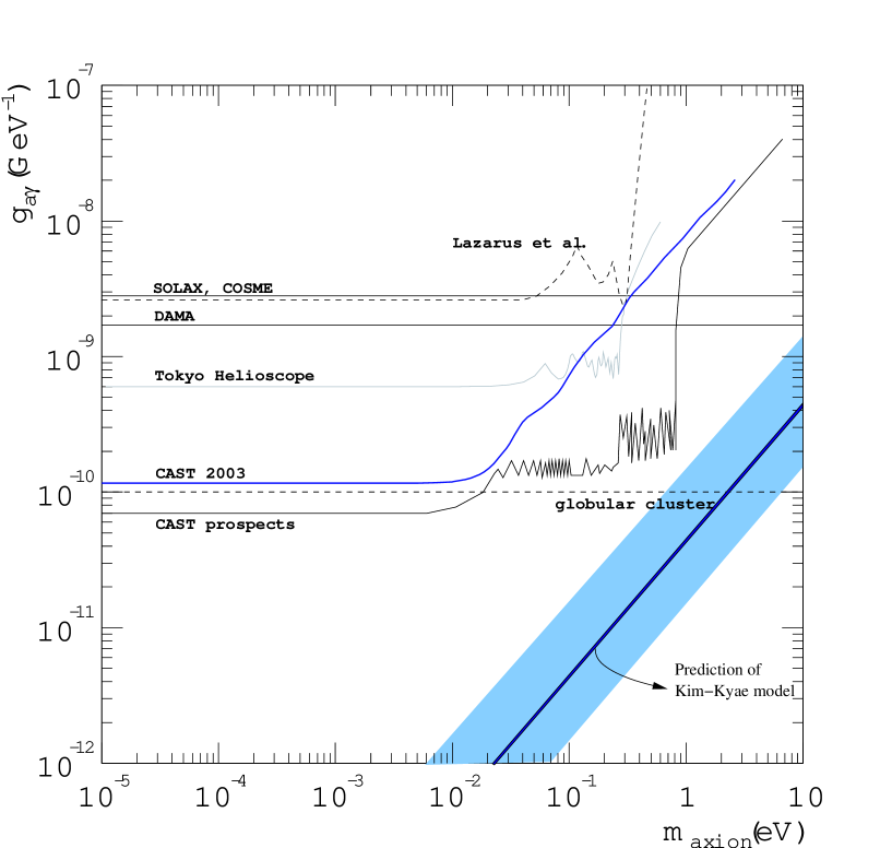
Figure 2: Experimental bound from various experiments, especially including CAST 2003 data. This figure is taken from the result paper of CAST experiment [31]. Here,we show the prediction of ${\bf Z}_{12}$ model by the thick line. The blue band is the 20 % theoretical error of Ref. [45].

For the electromagnetic field $F_{\rm em}^{\mu\nu}$, we have the following anomaly

$$\frac{1}{32\pi^{2}} \left(\frac{{-15}a_{\rm an}}{\tilde{V}}F_{\rm em}\tilde{F}_{\rm em}\right)$$

$$\simeq\frac{1}{32\pi^{2}}\left(\frac{{-15}(4\tilde{a}_{C}+\frac{16}{9}\sqrt{\epsilon}\tilde{a}_{s})}{4V_{1}}\right)F_{\rm em}\tilde{F}_{\rm em}\simeq\frac{1}{32\pi^{2}}\left(\frac{{-15}\tilde{a}_{C}}{V_{1}}\right)F_{\rm em}\tilde{F}_{\rm em}$$ (144)

$$=-\frac{1}{32\pi^{2}}\left(\frac{5}{3}\frac{a_{\rm QCD}}{F_{1}}\right)F_{\rm em}\tilde{F}_{\rm em}$$ (145)

whence we obtain the following high energy value for the axion-photon-photon coupling,

$${\cal L}_{a\gamma\gamma}=\tilde{c}_{a\gamma\gamma}\frac{a_{\rm QCD}}{F_{a,\rm QCD}}\left(\frac{e^{2}}{32\pi^{2}}F_{\rm em}\tilde{F}_{\rm em}\right)$$ (146)

where

$$\tilde{c}_{a\gamma\gamma}=\textstyle\frac{5}{3},\quad F_{a,\rm QCD}=F_{1}.$$ (147)

The axion-photon-photon coupling at low energy takes into account the QCD chiral symmetry breaking and we obtain

$$c_{a\gamma\gamma}=\tilde{c}_{a\gamma\gamma}-c_{\chi SB}\simeq-0.26$$ (148)

where we take $c_{\chi SB}\simeq 1.93$. The value $c_{\chi SB}$ depends on the current quark mass ratio $Z=m_{u}/m_{d}$, the instanton contribution factor $\xi=m_{s}/\Lambda_{\rm instanton}$, and $r_{ds}=m_{d}/m_{s}$. For $\xi=0.1$ and $r_{ds}=\frac{1}{20}$, we obtain

$$c_{\chi SB}=\frac{\frac{2}{3}(4+1.05Z)}{1+1.05Z}.$$ (149)

Inclusion of one-loop effects and second order chiral perturbation give sizable contributions to squared meson masses [45]. For $Z=\frac{5}{9}$, we obtain $c_{\chi SB}=1.93$. With the next order effect up to the 20% level, we obtain a band for $c_{\chi SB}$, i.e. $c_{\chi SB}=1.76\sim 2.26$. Thus, $c_{a\gamma\gamma}$ turns out to be sizable, which can be detected. Fig. 2 shows the current experimental search limit on $c_{a\gamma\gamma}$ and the prediction point of the present model with the band shown. The solid line corresponds to $c_{\chi SB}=1.93$. It is the first reliable calculation of the axion-photon-photon coupling. The cavity detectors [46] and the high $Z$ Rydberg atom Kyoto axion detector [47] already used this kind of axion-photon-photon interaction. But the recent CAST detector [31] seems to be the most promising one for detection of a very light axion in the region $F_{a}\sim 10^{11}$ GeV. The detectability of axion using the $c_{a\gamma\gamma}$ coupling was proposed by Sikivie [48]. However, the magnitude of $F_{a,\rm QCD}$ in the model we studied is at the GUT scale and it cannot be detected in these kinds of detectors.

What will be the case if we use VEVs of all the fields instead of just $C_{6}^{0}$ and $s_{4}^{0}$? We have discussed at length that it was not possible to find a global symmetry which has the QCD anomaly consistently with the breaking scheme of the flipped SU(5). More importantly, the hidden sector axion potential is higher than the QCD axion potential and the cross theorem dictates that the decay constant of the QCD axion is the breaking scale of U(1)_an. Thus, in our model the QCD axion cannot be made detectable.

Finally, we mention that the hidden sector axion potential can be made smaller than the QCD axion potential by making the hidden sector quark mass extremely small in which case the cross theorem acts in the other direction. In this case, we can expect that the QCD axion can fall in the detectable region. However, we have not found any approximate global symmetry possessing SU(5) anomaly and hence this desirable scenario is not realized in the present model.

6 Conclusion

In this paper, we presented a general method to house a QCD axion in string-derived MSSM models. One related objective is to make it observable in ongoing or future axion search experiments since the axion derived from superstring might be the most significant prediction of string. We presented the criteria that should be satisfied in these models. Since the magnitude of the axion decay constant is essential in the solution of the strong CP problem, cosmology, and in axion search experiments, we presented a general formula for the decay constant in Eqs. (7) and (9). We must consider the full Yukawa coupling structure of matter fields toward this objective. So far, this kind of full Yukawa coupling structure has not been studied except in a recent ${\bf Z}_{12-I}$ model [27]. Here the Yukawa coupling has been given completely, which made it possible for us to pick up an approximate global symmetry so that a phenomenologically allowed QCD axion results. However, in the ${\bf Z}_{12-I}$ model we study there does not exists a vacuum where $F_{a}\sim 10^{11}$ GeV with successful MSSM phenomenology. This might be a most probable situation in string models. It will be very interesting if one can find a string model with an observable QCD axion.

References

• [1]
• [2] P. G. Harris et al., New experimental limit on the electric dipole moment of the neutron, Phys. Rev. Lett.  82 (1999) 904.
• [3] J. E. Kim, Light Pseudoscalars, Particle Physics and Cosmology, Phys. Rept.  150 (1987) 1.
• [4] R. D. Peccei and H. R. Quinn, CP Conservation In The Presence Of Instantons, Phys. Rev. Lett.  38 (1977) 1440.
• [5] S. Weinberg, A New Light Boson?, Phys. Rev. Lett.  40 (1978) 223;
F. Wilczek, Problem Of Strong P And T Invariance In The Presence Of Instantons, Phys. Rev. Lett.  40 (1978) 279.
• [6] J. E. Kim, Weak Interaction Singlet And Strong CP Invariance, Phys. Rev. Lett.  43 (1979) 103;
M. A. Shifman, A. I. Vainshtein and V. I. Zakharov, Can Confinement Ensure Natural CP Invariance Of Strong Interactions?, Nucl. Phys. B 166 (1980) 493 ;
A. R. Zhitnitsky, On Possible Suppression Of The Axion Hadron Interactions. (In Russian), Sov. J. Nucl. Phys.  31 (1980) 260 [Yad. Fiz.  31 (1980) 497];
M. Dine, W. Fischler and M. Srednicki, A Simple Solution To The Strong CP Problem With A Harmless Axion, Phys. Lett. B 104 (1981) 199.
• [7] S. Y. Pi, Inflation Without Tears, Phys. Rev. Lett.  52 (1984) 1725 ;
M. Tegmark, A. Aguirre, M. Rees and F. Wilczek, Dimensionless constants, cosmology and other dark matters, Phys. Rev. D 73 (2006) 023505 [arXiv:astro-ph/0511774].
• [8] E. Witten, Some Properties Of O(32) Superstrings, Phys. Lett. B 149 (1984) 351.
• [9] E. Witten, Cosmic Superstrings, Phys. Lett. B 153 (1985) 243.
• [10] K. Choi and J. E. Kim, Harmful Axions In Superstring Models, Phys. Lett. B 154 (1985) 393 [Erratum-ibid.  156B (1985) 452].
• [11] X. G. Wen and E. Witten, World Sheet Instantons And The Peccei-Quinn Symmetry, Phys. Lett. B 166 (1986) 397.
• [12] J. Polchinski, private communication, August, 2006.
• [13] J. P. Conlon, The QCD axion and moduli stabilisation, JHEP 0605 (2006) 078 [arXiv:hep-th/0602233].
• [14] P. Svrcek and E. Witten, Axions in string theory, JHEP 0606 (2006) 051 [arXiv:hep-th/0605206].
• [15] I. W. Kim and J. E. Kim, Modification of decay constants of superstring axions: Effects of flux compactification and axion mixing, Phys. Lett. B 639 (2006) 342 [arXiv:hep-th/0605256].
• [16] T. Flacke, B. Gripaios, J. March-Russell and D. Maybury, Warped axions, arXiv:hep-ph/0611278.
• [17] K. Choi and K. S. Jeong, String theoretic QCD axion with stabilized saxion and the pattern of supersymmetry breaking, arXiv:hep-th/0611279.
• [18] P. Candelas, G. T. Horowitz, A. Strominger and E. Witten, Vacuum Configurations For Superstrings, Nucl. Phys. B 258 (1985) 46.
• [19] L. J. Dixon, J. A. Harvey, C. Vafa and E. Witten, Strings On Orbifolds, Nucl. Phys. B 261 (1985) 678;
Strings On Orbifolds. 2, Nucl. Phys. B 274 (1986) 285.
• [20] S. M. Barr, Harmless Axions In Superstring Theories, Phys. Lett. B 158 (1985) 397 ;
• [21] M. Dine, N. Seiberg and E. Witten, Fayet-Iliopoulos Terms in String Theory, Nucl. Phys. B 289 (1987) 589 ;
J. J. Atick, L. J. Dixon and A. Sen, String Calculation Of Fayet-Iliopoulos D Terms In Arbitrary Supersymmetric Compactifications, Nucl. Phys. B 292 (1987) 109 ;
M. Dine, I. Ichinose and N. Seiberg, F Terms And D Terms In String Theory, Nucl. Phys. B 293 (1987) 253.
• [22] M. B. Green and J. H. Schwarz, Anomaly Cancellation In Supersymmetric D=10 Gauge Theory And Superstring Theory, Phys. Lett. B 149 (1984) 117.
• [23] G. ’t Hooft, Renormalizable Lagrangians for Massive Yang-Mills Fields, Nucl. Phys. B 35 (1971) 167.
• [24] J. E. Kim, The Strong CP Problem in Orbifold Compactifications and an SU(3)$\times$SU(2)$\times$U(1)n Model, Phys. Lett. B 207 (1988) 434.
• [25] G. Lazarides, C. Panagiotakopoulos and Q. Shafi, Phenomenology And Cosmology With Superstrings, Phys. Rev. Lett.  56 (1986) 432.
• [26] M. Kamionkowski and J. March-Russell, Planck scale physics and the Peccei-Quinn mechanism, Phys. Lett. B 282 (1992) 137 [arXiv:hep-th/9202003] ;
S. M. Barr and D. Seckel, Planck scale corrections to axion models, Phys. Rev. D 46 (1992) 539.
• [27] J. E. Kim and B. Kyae, String MSSM through flipped SU(5) from Z(12) orbifold, arXiv:hep-th/0608085 ;
J. E. Kim and B. Kyae, Flipped SU(5) from Z(12-I) orbifold with Wilson line, arXiv:hep-th/0608086.
• [28] T. Kobayashi, S. Raby and R. J. Zhang, Searching for realistic 4d string models with a Pati-Salam symmetry: Orbifold grand unified theories from heterotic string compactification on a Z(6) orbifold, Nucl. Phys. B 704 (2005) 3 [arXiv:hep-ph/0409098] ;
W. Buchmuller, K. Hamaguchi, O. Lebedev and M. Ratz, Supersymmetric standard model from the heterotic string, Phys. Rev. Lett.  96 (2006) 121602 [arXiv:hep-ph/0511035].
• [29] J. E. Kim, Axion and almost massless quark as ingredients of quintessence, JHEP 9905 (1999) 022 [arXiv:hep-ph/9811509] ;
J. E. Kim, Model-dependent axion as quintessence with almost massless hidden sector quarks, JHEP 0006 (2000) 016 [arXiv:hep-ph/9907528].
• [30] K. Choi and J. E. Kim, Compactification And Axions In E(8)$\times$E(8)-Prime Superstring Models, Phys. Lett. B 165 (1985) 71.
• [31] K. Zioutas et al. [CAST Collaboration], First results from the CERN axion solar telescope (CAST), Phys. Rev. Lett.  94 (2005) 121301 [arXiv:hep-ex/0411033].
• [32] J. E. Kim and H. P. Nilles, The Mu Problem And The Strong CP Problem, Phys. Lett. B 138 (1984) 150.
• [33] J. E. Kim, A Common Scale For The Invisible Axion, Local Susy Guts And Saxino Decay, Phys. Lett. B 136 (1984) 378.
• [34] G. F. Giudice and A. Masiero, A Natural Solution to the mu Problem in Supergravity Theories, Phys. Lett. B 206 (1988) 480.
• [35] J. A. Casas and C. Munoz, Phys. Lett. B 306 (1993) 288 [arXiv:hep-ph/9302227].
• [36] J. E. Kim and H. P. Nilles, Symmetry principles toward solutions of the mu problem, Mod. Phys. Lett. A9 (1994) 3575 .
• [37] C. Vafa and E. Witten, Parity Conservation In QCD, Phys. Rev. Lett.  53 (1984) 535.
• [38] J. Preskill, M. B. Wise and F. Wilczek, Cosmology of the invisible axion, Phys. Lett. B 120 (1983) 127 ;
L. F. Abbott and P. Sikivie, A cosmological bound on the invisible axion, Phys. Lett. B 120 (1983) 133 ;
M. Dine and W. Fischler, The not-so-harmless axion, Phys. Lett. B 120 (1983) 137.
• [39] P. Sikivie, Of Axions, Domain Walls And The Early Universe, Phys. Rev. Lett.  48 (1982) 1156.
• [40] K. Choi and J. E. Kim, Domain Walls In Superstring Models, Phys. Rev. Lett.  55 (1985) 2637.
• [41] K.-S. Choi and J. E. Kim, Quarks and Leptons from Orbifolded Superstring (Springer-Verlag, Heidelberg, Germany, 2006).
• [42] S. Hamidi and C. Vafa, Interactions on Orbifolds, Nucl. Phys. B 279 (1987) 465 ;
L. J. Dixon, D. Friedan, E. J. Martinec and S. H. Shenker, The Conformal Field Theory Of Orbifolds, Nucl. Phys. B 282 (1987) 13 ;
D. Friedan, E. J. Martinec and S. H. Shenker, Conformal Invariance, Supersymmetry And String Theory, Nucl. Phys. B 271 (1986) 93 ;
T. Kobayashi and N. Ohtsubo, Yukawa Coupling Condition of Z(N) Orbifold Models, Phys. Lett. B 245 (1990) 441.
• [43] A. Masiero, D. V. Nanopoulos, K. Tamvakis and T. Yanagida, Ordinary SU(5) Predictions From A Supersymmetric SU(5) Model, Phys. Lett. B 115 (1982) 298.
• [44] G. ’t Hooft, Computation of the quantum effects due to a four-dimensional pseudoparticle, Phys. Rev. D 14 (1976) 3432 [Erratum-ibid. D 18 (1978) 2199].
• [45] D. B. Kaplan and A. V. Manohar, Current Mass Ratios Of The Light Quarks, Phys. Rev. Lett.  56 (1986) 2004.
• [46] S. De Panfilis et al., Limits on the Abundance and Coupling of Cosmic Axions at 4.5-MicroeV $<$ M(a) $<$ 5.0-MicroeV, Phys. Rev. Lett.  59 (1987) 839 ;
C. Hagmann, P. Sikivie, N. S. Sullivan and D. B. Tanner, Results from a search for cosmic axions, Phys. Rev. D 42 (1990) 1297 ;
C. Hagmann et al., First results from a second generation galactic axion experiment, Nucl. Phys. Proc. Suppl.  51B (1996) 209 [arXiv:astro-ph/9607022].
• [47] S. Matsuki, talk presented at IDM-1998, Buxton, England, 7–11 Sep. 1997, Proc. $``$The identification of Dark Matter”, ed. N. J. C. Spooner and V. Kudryavtsev (World Scientific Pub. Co., Singapore, 1999) p. 441.
• [48] P. Sikivie, Experimental tests of the *invisible* axion, Phys. Rev. Lett.  51 (1983) 1415 [Erratum-ibid.  52 (1984) 695].