Sterile neutrino production via active-sterile oscillations: the quantum Zeno effect.

Abstract:

We study several aspects of the kinetic approach to sterile neutrino production via active-sterile mixing. We obtain the neutrino propagator in the medium including self-energy corrections up to $\mathcal{O}(G^{2}_{F})$, from which we extract the dispersion relations and damping rates of the propagating modes. The dispersion relations are the usual ones in terms of the index of refraction in the medium, and the damping rates are $\Gamma_{1}(k)=\Gamma_{aa}(k)\cos^{2}\theta_{m}(k);\Gamma_{2}(k)=\Gamma_{aa}(k)\sin^{2}\theta_{m}(k)$ where $\Gamma_{aa}(k)\propto G^{2}_{F}\,kT^{4}$ is the active neutrino scattering rate and $\theta_{m}(k)$ is the mixing angle in the medium. We provide a generalization of the transition probability in the medium from expectation values in the density matrix: $P_{a\rightarrow s}(t)=\frac{\sin^{2}2\theta_{m}}{4}\left[e^{-\Gamma_{1}t}+e^{-\Gamma_{2}t}-2e^{-\frac{1}{2}(\Gamma_{1}+\Gamma_{2})t}~{}\cos\big{(}\Delta Et\big{)}\right]$ and study the conditions for its quantum Zeno suppression directly in real time. We find the general conditions for quantum Zeno suppression, which for $m_{s}\sim\textrm{keV}$ sterile neutrinos with $\sin 2\theta\lesssim 10^{-3}$ may only be fulfilled near an MSW resonance. We discuss the implications for sterile neutrino production and argue that in the early Universe the wide separation of relaxation scales far away from MSW resonances suggests the breakdown of the current kinetic approach.

1 Introduction

Sterile neutrinos, namely weak interaction singlets, are ubiquitous in extensions of the standard model[1, 2, 3, 4] and are emerging as plausible cold or warm dark matter candidates[5, 6, 7, 8, 9, 10, 11, 12, 13, 14, 15, 17, 18], as potentially important ingredients in stellar collapse and supernovae[16, 19] and in primordial nucleosynthesis[20, 21]. Sterile neutrinos with masses in the range $\sim\mathrm{keV}$ may also provide an explanation of pulsar “kicks” via asymmetric neutrino emission[22, 23].

The MiniBooNE collaboration[24] has recently reported results in contradiction with those from LSND[25, 26] that suggested a sterile neutrino with $\Delta m^{2}\sim 1~{}\textrm{eV}^{2}$ scale. Although the MiniBooNE results hint at an excess of events below $475~{}\mathrm{MeV}$ the analysis distinctly excludes two neutrino appearance-only from $\nu_{\mu}\rightarrow\nu_{e}$ oscillations with a mass scale $\Delta m^{2}\sim 1~{}\textrm{eV}^{2}$, perhaps ruling out a light sterile neutrino. However, a recent analysis[27] suggests that while $(3+1)$ schemes are strongly disfavoured, $(3+2)$ neutrino schemes provide a good fit to both the LSND and MiniBooNE data, including the excess of low energy events, because of the possibility of CP violation in these schemes, although significant tension remains between appearance and disappearance experiments.

Sterile neutrinos as dark matter candidates would require masses in the $\mathrm{keV}$ range[5, 6, 7, 8, 9, 10, 11, 13, 15, 17, 18], and their radiative decay would contribute to the X-ray background[9, 28]. Analysis from the X-ray background in clusters provide constraints on the masses and mixing angles of sterile neutrinos[13, 29, 30, 31], and recently it has been suggested that precision laboratory experiments on $\beta$ decay in tritium may be sensitive to $\sim\textrm{keV}$ neutrinos[32].

Sterile neutrinos couple to standard model active neutrinos through an off diagonal mass matrix, therefore they are produced via active-sterile mixing. In the hot and dense environment of the early Universe when the scattering rate of active neutrinos off the thermal medium is large, namely a short mean free path, there is a competition between the oscillation length and the mean free path. It is expected that when the oscillation length is much larger than the mean free path, the active to sterile transition probability is hindered because rapid scattering events “freeze” the state to the active flavor state. This phenomenon receives the name of quantum Zeno effect or Turing’s paradox, studied early in quantum optical coherence[33] but considered within the context of neutrino oscillations in a medium in references[34, 35, 36]. Pioneering work on the description of neutrino oscillations and decoherence in a medium was cast in terms of kinetic equations for a flavor “matrix of densities”[37] or in terms of $2\times 2$ Bloch-type equations for flavor quantum mechanical states[34, 38]. A general field theoretical approach to neutrino mixing and kinetics was presented in [35, 36, 4, 16], however, while such approach in principle yields the time evolution of the distribution functions, sterile neutrino production in the early Universe is mostly studied in terms of simple phenomenological rate equations[5, 8, 40, 39, 41, 42]. An early approach[40] relied on a Wigner-Weisskopf effective Hamiltonian for the quantum mechanical states in the medium, while numerical studies of sterile neutrinos as possible dark matter candidates[8, 42] rely on an approximate approach which inputs an effective production rate in terms of a time averaged transition probability[39, 41] and relies on the following semiphenomenological rate equation[40, 41, 42, 43, 8]

$$\frac{d}{dt}f_{s}(p,t)\approx\Gamma(a\rightarrow s;p)\left[f_{a}(p;t)-f_{s}(p;t)\right]$$ (1)

where $f_{a,s}$ are the distribution functions for active (a) and sterile (s) neutrinos, $d/dt$ is the total time derivative including the redshift of momenta through the expansion in the early Universe and $\Gamma(a\rightarrow s;p)$ is an effective reaction rate. It is determined to be[40, 41]

$$\Gamma(a\rightarrow s;p)\approx\frac{\Gamma_{aa}(p)}{2}\Big{\langle}P_{a\rightarrow s}\Big{\rangle}$$ (2)

where $\Gamma_{aa}(p)\sim G^{2}_{F}\,p\,T^{4}$ is the active neutrino reaction rate and $\Big{\langle}P_{a\rightarrow s}\Big{\rangle}$ is a time average of the active-sterile transition probability in the medium which in reference[41] is given by

$$\Big{\langle}P_{a\rightarrow s}\Big{\rangle}=\frac{\Gamma_{aa}}{2}\int^{\infty}_{0}P_{a\rightarrow s}(t)dt$$ (3)

with $P_{a\rightarrow s}$ the usual quantum mechanical transition probability but exponentially damped by a decoherence factor[41]

$$P_{a\rightarrow s}(t)=\frac{\sin^{2}2\theta_{m}}{2}~{}e^{-\frac{\Gamma_{aa}}{2}t}~{}\left[1-\cos(\Delta Et)\right]$$ (4)

where $\Delta E,\theta_{m}$ are the oscillation frequency and mixing angle in the medium respectively and $\tau_{dec}=2/\Gamma_{aa}$ is the decoherence time scale. Hence the rate that enters in the kinetic equation (1) is given by[41]

$$\Gamma(a\rightarrow s;p)=\frac{\Gamma_{aa}(p)}{4}\frac{\sin^{2}2\theta_{m}(p)~{}\Big{(}\frac{2\,\Delta E(p)}{\Gamma_{aa}(p)}\Big{)}^{2}}{\Big{[}1+\Big{(}\frac{2\,\Delta E(p)}{\Gamma_{aa}(p)}\Big{)}^{2}\Big{]}}$$ (5)

where $\theta_{m}(p),\Delta E(p)$ are the mixing angle and active-sterile oscillation frequency in the medium respectively. The quantum Zeno paradox is manifest in the ratio $2\Delta E(p)/\Gamma_{aa}(p)$ in (5): for a relaxation time shorter than the oscillation time scale, or mean free path smaller than the oscillation length, $\Gamma_{aa}(p)\gg\Delta E(p)$ and the active-sterile transition probability is suppressed, with a concomitant reduction of the sterile production rate in the kinetic equation (1). Most studies[8, 42] of the production of sterile neutrinos via active-sterile mixing rely on the kinetic description afforded by equation (1).

A field theoretic approach to sterile neutrino production near a MSW resonance which focuses primarily on the hadronic contribution and seemingly yields a different rate has been proposed in reference[44], and more recently it has been observed that quantum Zeno suppression may have important consequences in thermal leptogenesis[45].

Questions and goals: Recently we have studied the non-equilibrium aspects of oscillations and damping in a model of mesons that effectively describes the dynamics of mixed neutrinos in a medium in thermal equilibrium[46]. In the case of two species of “neutrinos” this study reveals that there are two propagating modes in the medium, whose dispersion relations feature the index of refraction correction from forward scattering similar to those for neutrinos in the medium but also two different damping rates which are determined by the imaginary part of the self-energy correction evaluated on the mass shell. For the case of two mixed neutrinos in a medium it is natural to expect that the imaginary part of the self-energy corrections evaluated on the mass shell (dispersion relations) yield two different damping rates. Thus the results of ref.[46] lead us to expect that for one active and one sterile mixed neutrinos the propagating modes in the medium feature two different damping rates and this observation motivates the first question: How does the active-sterile transition probability $P_{a\rightarrow s}(t)$ account for two damping scales?, namely why does the result (4) feature only one damping scale?. This question leads to the related second question: How to generalize the concept of a transition probability to the case of propagation in a medium?. The usual transition probability is based on the evolution of single particle quantum mechanical wavefunctions which are linear superpositions of the eigenstates of the Hamiltonian. The statistical description of a medium does not rely on single particle wavefunctions or quantum mechanical states but on the quantum density matrix. Therefore the concept of the active-sterile transition probability $P_{a\rightarrow s}(t)$ in a medium must be generalized in terms of the quantum density matrix. As discussed above the final expression for the effective sterile production rate (5) exhibits the Quantum Zeno suppression whenever $\Gamma_{aa}(p)\gg\Delta E(p)$ which has been argued to be the case at high temperature[8]. From the quantum field theory perspective this possibility is puzzling for the following reason: at high temperature the difference in the oscillation frequencies $\Delta E(p)$ is determined by the index of refraction correction from forward scattering[47] in the medium. This is determined by a one-loop contribution[47] and is formally of order $G_{F}$, whereas the interaction rate $\Gamma_{aa}$ arises from an absorptive part of the self-energy and in the effective Fermi’s field theory is at least of two-loop order, formally of order $G^{2}_{F}$. Therefore from the field theoretical perspective quantum Zeno suppression requires a competition of terms of different order in the perturbative expansion in Fermi’s effective field theory[48]. This observation brings us to the third question: considering and active neutrino with standard model interactions, can quantum Zeno suppression be manifest at high temperatures within the regime of validity of the perturbative expansion?.

The emerging cosmological and astrophysical importance of sterile neutrinos motivates a deeper scrutiny of the current approach to the dynamical aspects of their production based on the rate equation (1) with the effective rate(5). While at this stage we take this description based on (1-3) for granted, our goal is to address the three questions enunciated above within the quantum field theory of mixed neutrinos with standard model interactions in the medium, and in so doing we scrutinize the reliability of this approach. Our goals in this article are: i: to provide a quantum field theoretical understanding of the dispersion relations and damping rates of the two propagating modes (quasiparticles) in the medium, ii: to provide a generalization of the active-sterile transition probability in real time in the medium and a reassessment of the time averaged transition probability $\langle P_{a\rightarrow s}\rangle$ directly from the non-equilibrium time evolution of the full density matrix and iii: to scrutinize the possibility of quantum Zeno suppression within the realm of validity of perturbation theory with standard model interactions for the active neutrino.

Main results:

We consider one active and one sterile neutrino[21] to highlight the main conceptual aspects. Unlike most treatments in the literature that study the dynamics in terms of Bloch-type equations for a $2\times 2$ flavor density matrix[34, 41, 14], we study the full quantum field theoretical density matrix. A main advantage of studying the time evolution of the density matrix directly within the quantum field theory context is that we obtain the neutrino propagator which yields the quasiparticle dispersion relations and damping rates in the medium. Furthermore, the time evolution of the quantum field density matrix allows to study the non-equilibrium dynamics of neutrino mixing and propagation as an initial value problem from which we obtain the dispersion relation of the correct quasiparticle modes in the medium, their damping rates (widths) and the generalization of the active-sterile transition probability. These are all determined by the neutrino propagator in the medium which includes self-energy corrections up to two loops $\mathcal{O}(G^{2}_{F})$ in the standard model weak interactions. Our main results are the following:

• There are two quasiparticle propagating modes, their dispersion relations are the usual ones in terms of the index of refraction in the medium[47] plus perturbative radiative corrections of $\mathcal{O}(G^{2}_{F})$ and their damping rates are given by $\Gamma_{1}(p)=\Gamma_{aa}(p)\cos^{2}\theta_{m}(p)~{};~{}\Gamma_{2}(p)=\Gamma_{aa}(p)\sin^{2}\theta_{m}(p)$ where $\Gamma_{aa}(p)\propto G^{2}_{F}\,p\,T^{4}$ is the active neutrino scattering rate in the absence of mixing, and $\theta_{m}(p)$ the mixing angle in the medium. We provide a physical interpretation of these different quasiparticle relaxation rates and argue that these must naturally be correct in agreement with the fact that sterile neutrinos are much more weakly coupled to the plasma than active neutrinos in the regimes far away from an MSW resonance.

• We generalize the concept of the active-sterile transition probability $P_{a\rightarrow s}(t)$ in the medium from expectation values of the active and sterile neutrino field operators in the full quantum density matrix. This is achieved by furnishing an initial value problem via linear response: the density matrix is initialized to feature an non-vanishing expectation value of the active neutrino field, but a vanishing expectation value of the sterile field. Upon time evolution a non-vanishing expectation value of the sterile neutrino field develops from which we extract unambiguously the transition probability. This formulation directly inputs the neutrino propagator with self-energy corrections up to $\mathcal{O}(G^{2}_{F})$. We find

  $$P_{a\rightarrow s}(t)=\frac{\sin^{2}2\theta_{m}}{4}\left[e^{-\Gamma_{1}t}+e^{-\Gamma_{2}t}-2e^{-\frac{1}{2}(\Gamma_{1}+\Gamma_{2})t}~{}\cos\big{(}\Delta Et\big{)}\right]$$ (6)

  This expression identifies the decoherence time scale for suppression of the interference term $\tau_{dec}=2/(\Gamma_{1}+\Gamma_{2})=2/\Gamma_{aa}$. Although the oscillatory interference term in the active-sterile transition probability is suppressed on the decoherence time scale $\tau_{dec}$, far away from an MSW resonance the relevant time scale for suppression of $P_{a\rightarrow s}(t)$ is determined by the smaller of the relaxation scales for the quasiparticles $\Gamma_{1}(p)$ or $\Gamma_{2}(p)$. If the effective sterile production rate (2) is computed by inserting the result (6) into the time average (3) the result for the effective production rate is enhanced far away from MSW resonances compared to that given by (5). However we argue that the widely different damping rates $\Gamma_{1,2}$ suggest a breakdown of the simple rate equation (1) in these regimes in the early Universe.

• We provide a real time interpretation of the quantum Zeno suppression based on the generalization of the active-sterile transition probability (6). The complete general conditions for quantum Zeno suppression of the active-sterile transition probability are found to be:

  • a) the active neutrino scattering rate much larger than the oscillation frequency $\Gamma_{aa}(p)\gg\Delta E(p)$,

  • b) The relaxation rates of the propagating modes must be approximately equal. In the case under consideration with $\Gamma_{1}(p)=\Gamma_{aa}(p)\cos^{2}\theta_{m}(p)~{};~{}\Gamma_{2}(p)=\Gamma_{aa}(p)\sin^{2}\theta_{m}(p)$ this condition determines an MSW resonance in the medium.

  Although these conditions are general, for sterile neutrinos with $m_{s}\sim\textrm{keV}$ and $\sin 2\theta\lesssim 10^{-3}$ and standard model interactions for the active neutrino, we find that they may only be fulfilled near an MSW resonance at $T_{MSW}\sim 215\,\textrm{MeV}$, but a firm assessment of such possibility requires to include $\mathcal{O}(G^{2}_{F})$ corrections to the index of refraction and a deeper assessment of the perturbative expansion. Far away from the resonance either at high or low temperature there is a wide separation between the two relaxation rates of the propagating modes in the medium. In these cases the transition probability reaches a maximum on the decoherence time scale $\tau_{dec}=2/\Gamma_{aa}$, and is suppressed on a much longer time scale determined by the smaller of the damping rates. Even for $\tau_{dec}\Delta E(k)\ll 1$, which in the literature [34, 8] is taken to indicate quantum Zeno suppression, we find that the transition probability is substantial on time scales much longer than $\tau_{dec}$ if $\Gamma_{1}$ and $\Gamma_{2}$ are widely separated.

Section (2) provides a study of the time evolution of the full quantum field theory density matrix, and the equations of motion for expectation values of the neutrino fields. In this section we obtain the dispersion relations and widths of the propagating modes (quasiparticles) in the medium up to second order in the weak interactions. In section (3) we introduced the generalized transition probability in the medium from the time evolution of expectation values of neutrino field operators in the density matrix. In this section we discuss in detail the conditions for the quantum Zeno effect, both in real time and in the time-averaged transition probability and the possibility of quantum Zeno suppression within the realm of validity of perturbation theory in standard model weak interactions. In section (4) we discuss the implications of our results for the production of sterile neutrinos in the early Universe. In this section we argue that the in the early Universe far away from an MSW resonance the wide separation of the damping scales makes any definition of the time averaged transition probability ambiguous, and question the validity of the usual rate equation to describe sterile neutrino production in the early Universe far away from MSW resonances. Section (5) presents our conclusions .

2 Quantum field theory treatment in the medium

2.1 Non-equilibrium density matrix

In a medium the relevant question is not that of the time evolution of a pure quantum state, but more generally that of a density matrix from which expectation values of suitable operators can be obtained.

In order to provide a detailed understanding of the quantum Zeno effect, we need a reliable estimate of the dispersion relations and the damping rates of the propagating modes in the medium which are determined by the complex poles of the neutrino propagator in the medium.

In this article we obtain these from the study of the real time evolution of the full density matrix by implementing the methods of quantum field theory in real time described in references[49, 50, 51, 52, 53, 46]. This is achieved by introducing external (Grassmann) sources that induce an expectation value for the neutrino fields. Upon switching off the sources these expectation values relax towards equilibrium and their time evolution reveals both the correct energy and the relaxation rates[53, 46]. The main ingredient in this program is the active neutrino self-energy which we obtain up to second order in the standard model weak interactions.

We consider a model of one active and one sterile Dirac neutrinos in which active-sterile mixing is included via an off diagonal Dirac mass matrix and the active neutrino only features standard model weak interactions. The relevant Lagrangian density is given by

$$\mathcal{L}=\mathcal{L}^{0}_{\nu}+\mathcal{L}_{Ia}\,,$$ (7)

where

$$\mathcal{L}^{0}_{\nu}=\overline{\nu}\left(i{\not\!{\partial}}\,\mathbb{I}-\mathbb{M}\right)\nu\,,$$ (8)

with $\nu$ being the neutrino doublet

$$\nu\equiv\left(\begin{array}[]{c}\nu_{a}\\ \nu_{s}\\ \end{array}\right)\,,$$ (9)

and $a,s$ refer to the flavor indexes of the active and sterile neutrinos respectively.

The neutrino fields are four component Dirac spinors $\nu=\nu_{R}+\nu_{L}$ with $R,L$ the right and left handed components, both for $a,s$. The mass matrix in (8) is of the Dirac type: $\overline{\nu_{R}}\,\mathbb{M}\,\nu_{L}+\mathrm{h.c.}$.

The Dirac mass matrix $\mathbb{M}$ is given by

$$\mathbb{M}=\left(\begin{array}[]{cc}m_{aa}&m_{as}\\ m_{as}&m_{ss}\\ \end{array}\right)\,.$$ (10)

It can be diagonalized by the unitary transformation that takes flavor into mass eigenstates, namely

$$\left(\begin{array}[]{c}\nu_{a}\\ \nu_{s}\\ \end{array}\right)=U(\theta)\left(\begin{array}[]{c}\nu_{1}\\ \nu_{2}\\ \end{array}\right)\,,$$ (11)

with the unitary transformation given by the $2\times 2$ matrix

$$U(\theta)=\left(\begin{array}[]{cc}\cos\theta&\sin\theta\\ -\sin\theta&\cos\theta\\ \end{array}\right)\,.$$ (12)

In this basis the mass matrix is diagonal

$$\mathbb{M}=\left(\begin{array}[]{cc}M_{1}&0\\ 0&M_{2}\\ \end{array}\right)\,,$$ (13)

with the relation

$$m_{aa}=\cos^{2}\theta M_{1}+\sin^{2}\theta M_{2}~{}~{};~{}~{}m_{ss}=\sin^{2}\theta M_{1}+\cos^{2}\theta M_{2}~{}~{};~{}~{}m_{as}=\frac{1}{2}(M_{2}-M_{1})\sin 2\theta\,,$$ (14)

where $\theta$ is the vacuum mixing angle. The Lagrangian density $\mathcal{L}_{Ia}$ describes the weak interactions of the active neutrino $\nu_{a}$ with hadrons or quarks and its associated charged lepton. Leptons, hadrons or quarks reach equilibrium in a thermal bath on time scales far shorter than those of neutrinos, therefore in what follows we assume these degrees of freedom to be in thermal equilibrium. Furthermore, in our analysis we will not include the non-linearities associated with a neutrino background, such component requires a full non-equilibrium treatment and is not germane to the focus of this study. The Lagrangian density that includes both charged and neutral current interactions can be written in the form[36, 16, 4]

$$\mathcal{L}_{Ia}=\frac{G_{F}}{\sqrt{2}}~{}\left[\overline{\mathcal{O}}_{a}L\nu_{a}+\mathrm{h.c.}+\overline{\nu}_{a}\gamma_{\mu}J^{\mu}L\nu_{a}\right]$$ (15)

where $L=(1-\gamma^{5})/2$, the current $J^{\mu}$ includes both charge and neutral current contributions from the background in thermal equilibrium. For example the following charged and neutral current contributions to the effective Lagrangian (taking the active to be, for example, the electron neutrino):

$$-\frac{G_{F}}{\sqrt{2}}\Bigg{\{}4[\overline{\nu}_{e}\gamma^{\mu}Le][\overline{e}\gamma_{\mu}L\nu_{e}]+2\overline{\nu}_{e}\gamma^{\mu}[\overline{e}\gamma_{\mu}(g_{V}-g_{A}\gamma^{5})e]L\nu_{e}\Bigg{\}}\,,$$ (16)

the first term (from charged currents) can be Fierz-rearranged to yield the form of the second term in (15). This term yields a contribution to the index of refraction in the medium[47], $\mathcal{O}_{a}$ describes the charged current interaction with hadrons or quarks and the charged lepton, for example[36, 4] $\mathcal{O}_{a}=\gamma^{\mu}L\psi_{e}\overline{\psi}_{n}\gamma_{\mu}(C_{V}-C_{A}\gamma^{5})\psi_{p}$. In the case of all active species the neutral current contribution to $J^{\mu}$ is the same for all flavors (when the neutrino background is neglected), hence it does not contribute to oscillations and the effective matter potential. In the case in which there are sterile neutrinos, which do not interact with the background directly, the neutral current contribution does contribute to the medium modifications of active-sterile mixing angles and oscillations frequencies.

To study the dynamics in a medium we must consider the time evolution of the density matrix. While the usual approach truncates the full density matrix to a $2\times 2$ “flavor” subspace thus neglecting all but the flavor degrees of freedom, and studies its time evolution in terms of Bloch-type equations[34, 41], our study relies instead on the time evolution of the full quantum field theoretical density matrix.

The full density matrix describes a statistical ensemble of neutrinos and charged leptons, quarks or hadrons, these latter degrees of freedom are in thermal equilibrium and constitute the thermal bath. The fact that the density matrix describes charged leptons, quarks and or hadrons in statistical equilibrium will be used below (see eqns. 27, 28 ) when the correlation functions of these fields are obtained from ensemble averages in the density matrix.

The time evolution of the quantum density matrix $\hat{\rho}$ is given by the quantum Liouville equation

$$i\frac{d\hat{\rho}(t)}{dt}=\left[H,\hat{\rho}(t)\right]$$ (17)

where $H$ is the full Hamiltonian with weak interactions. The solution is given by

$$\hat{\rho}(t)=e^{-iHt}\,\hat{\rho}(0)\,e^{iHt}$$ (18)

from which the time evolution of observables associated with an operator $\mathcal{A}$, namely its expectation value in the time evolved density matrix is given by

$$\langle\mathcal{A}(t)\rangle=\mathrm{Tr}\hat{\rho}(t)\mathcal{A}\,.$$ (19)

The density matrix elements in the field basis are given by

$$\hat{\rho}(\psi,\psi^{\prime};t)=\int\mathcal{D}\phi\mathcal{D}\phi^{\prime}\,\langle\psi|e^{-iHt}|\phi\rangle\,\hat{\rho}(\phi,\phi^{\prime};0)\,\langle\phi^{\prime}|e^{iHt}|\psi^{\prime}\rangle\,,$$ (20)

the matrix elements of the forward and backward time evolution operators can be handily written as path integrals and the resulting expression involves a path integral along a forward and backward contour in time. This is the Schwinger-Keldysh[49, 51, 50, 52] formulation of non-equilibrium quantum statistical mechanics which yields the correct time evolution of quantum density matrices in field theory. Expectation values of operators are obtained as usual by coupling sources conjugate to these operators in the Lagrangian and taking variational derivatives with respect to these sources. This formulation of non-equilibrium quantum field theory yields all the correlation and Green’s functions. Of primary focus is the neutrino retarded propagator

$$S_{\alpha\beta}(\vec{x}-\vec{x}^{\prime};t-t^{\prime})=-i\Theta(t-t^{\prime})~{}\mathrm{Tr}\hat{\rho}(0)\big{\{}\psi_{\alpha}(\vec{x},t),\overline{\psi}_{\beta}(\vec{x^{\prime}},t^{\prime})\big{\}}\,,$$ (21)

where the flavor indices $\alpha,\beta$ correspond to either active or sterile and $\psi_{\alpha}(\vec{x},t)$ is a neutrino field in the Heisenberg picture. The (complex) poles in complex frequency space of the spatio-temporal Fourier transform of the neutrino propagator yields the dispersion relations and damping rates of the quasiparticle states in the medium. It is not clear if this important information can be extracted from the truncated $2\times 2$ density matrix in flavor space usually invoked in the literature and which forms the basis of the kinetic description (1), but certainly the full quantum field density matrix does have all the information on the correct dispersion relations and relaxation rates.

A standard approach to obtain the propagation frequencies and damping rates of quasiparticle excitations in a medium is the method of linear response[54]. An external source $\eta$ is coupled to the field operator $\psi$ to induce an expectation value of this operator in the many body density matrix, the time evolution of this expectation value yields the quasiparticle dynamics, namely the propagation frequencies and damping rates. In linear response

$$\langle\psi_{\alpha}(\vec{x},t)\rangle\equiv\mathrm{Tr}~{}\hat{\rho}(0)\psi_{\alpha}(\vec{x},t)=-\int d^{3}x^{\prime}dt^{\prime}S_{\alpha\beta}(\vec{x}-\vec{x}^{\prime};t-t^{\prime})\,\eta_{\beta}(\vec{x}^{\prime},t^{\prime})\,,$$ (22)

where $S(\vec{x}-\vec{x}^{\prime};t-t^{\prime})$ is the retarded propagator or Green’s function (21) and averages are in the full quantum density matrix. The quasiparticle dispersion relations and damping rates are obtained from the complex poles of the spatio-temporal Fourier transform of the retarded propagator in the complex frequency plane[54, 55]. For one active and one sterile neutrino there are two propagating modes in the medium. Up to one loop order $\mathcal{O}(G_{F})$ the index of refraction in the medium yields two different dispersion relations[47], hence we expect also that the damping rates for these two propagating modes which will be obtained up to $\mathcal{O}(G^{2}_{F})$ will be different. This expectation will be confirmed below with the explicit computation of the propagator up to $\mathcal{O}(G^{2}_{F})$.

Linear response is the standard method to obtain the dispersion relations and damping rates of quasiparticle excitations in a plasma in finite temperature field theory[55]. The linear response relation (22) can be inverted to write

$$S^{-1}\langle\psi(\vec{x},t)\rangle=-\eta(\vec{x},t)\,,$$ (23)

where $S^{-1}$ is the (non-local) differential operator which is the inverse of the propagator, namely the effective Dirac operator in the medium that includes self-energy corrections. This allows to study the dynamics as an initial value problem and to recognize the quasiparticle dispersion relations and damping rates directly from the time evolution of expectation values of the field operators. This method has been applied to several different problems in quantum field theory out of equilibrium and the reader is referred to the literature for detailed discussions[56, 57, 58, 53, 46].

It is important to highlight that $\langle\psi(\vec{x},t)\rangle$ is not a single particle wave function but an ensemble average of the quantum field operator in the non-equilibrium density matrix, namely an ensemble average. In contrast to this expectation value, a single particle wave function is defined as $\langle 1|\psi(\vec{x},t)|0\rangle$ where $|0\rangle$ is the vacuum and $|1\rangle$ a Fock state with one single particle.

In the present case the initial value problem allows us also to study the time evolution of flavor off diagonal density matrix elements. Consider an external source $\eta_{a}$ that induces an initial expectation value only for the active neutrino field $\psi_{a}$, such an external source prepares the initial density matrix so that at $t=0$ the active neutrino field operator features a non-vanishing expectation value, while the sterile one has a vanishing expectation value. Upon time evolution the density matrix develops flavor off diagonal matrix elements and the sterile neutrino field $\psi_{s}$ develops an expectation value. The solution of the equation of motion (23) as an initial value problem allows us to extract precisely the time evolution of $\langle\psi_{s}\rangle$ from which we unambiguously extract the transition probability in the medium.

2.2 Equations of motion in linear response

The linear response approach to studying the non-equilibrium evolution relies on “adiabatically switching on” an external source $\eta$ that initializes the quantum density matrix to yield an expectation value for the neutrino field(s). Upon switching off the external source the expectation values of the neutrino fields relax to equilibrium. The real time evolution of the expectation values reveals the dispersion relations and damping rates of the propagating quasiparticle modes in the medium. These are determined by the poles of the retarded propagator in the complex frequency plane[54, 55].

The equation of motion for the expectation value of the flavor doublet is obtained by introducing external Grassmann-valued sources $\eta$[56, 57, 58]

$$\mathcal{L}_{S}=\overline{\nu}\,\eta+\overline{\eta}\,\nu\,,$$ (24)

shifting the field

$$\nu^{\pm}_{\alpha}=\psi_{\alpha}+\Psi^{\pm}_{\alpha}~{}~{};~{}~{}\psi_{\alpha}=\langle\nu^{\pm}_{\alpha}\rangle~{}~{};~{}~{}\langle\Psi^{\pm}_{\alpha}\rangle=0,$$ (25)

for $\alpha=a,s$, and imposing $\langle\Psi^{\pm}_{a}\rangle=0$ order by order in the perturbation theory [56, 57, 58]. Implementing this program we find the following equation of motion for the expectation value of the neutrino field $\psi_{\alpha}(\vec{x},t)=\mathrm{Tr}\big{[}\hat{\rho}(0)\nu_{\alpha}(\vec{x},t)\big{]}$ induced by the external field $\eta$

$$\left(i\not\!{\partial}\,\delta_{\alpha\beta}-M_{\alpha\beta}+\Sigma^{tad}_{\alpha\beta}L\right)\,\psi_{\beta}(\vec{x},t)+\int d^{3}x^{\prime}\int^{t}_{-\infty}dt^{\prime}\Sigma^{ret}_{\alpha\beta}(\vec{x}-\vec{x}^{\prime},t-t^{\prime})\psi_{\beta}(\vec{x}^{\prime},t^{\prime})=-\eta_{\alpha}(\vec{x},t),$$ (26)

The tadpole

$$\Sigma^{tad}=\frac{G_{F}}{\sqrt{2}}\gamma_{0}\,\mathrm{Tr}\widehat{\rho}(0)\,J^{0}(0,0)$$ (27)

describes the one-loop charged and neutral current contributions to the matter potential in the medium, and

$$\Sigma^{ret}_{aa}(\vec{x}-\vec{x^{\prime}};t-t^{\prime})=\frac{i\,G^{2}_{F}}{2}~{}\mathrm{Tr}\hat{\rho}(0)\Big{[}\mathcal{O}_{a}(\vec{x},t)\overline{\mathcal{O}}_{a}(\vec{x^{\prime}},t^{\prime})+\overline{\mathcal{O}}_{a}(\vec{x^{\prime}},t^{\prime})\mathcal{O}_{a}(\vec{x},t)\Big{]}\,.$$ (28)

The latter describes the two-loops diagrams with intermediate states of hadrons or quarks and the charged lepton, it is a fermionic correlation function in equilibrium and its spatio-temporal Fourier transform features an imaginary part that yields the relaxation rates of neutrinos in the medium. As shown in ref.[53], the spatial Fourier transform of the retarded self-energy can be written as

$$\Sigma^{ret}(\vec{k},t-t^{\prime})=\,\frac{i}{\pi}\int_{-\infty}^{\infty}dk_{0}\,\mathrm{Im}\Sigma(\vec{k},k_{0})\,e^{ik_{0}(t-t^{\prime})}\,.$$ (29)

The imaginary part $\mathrm{Im}\Sigma(\vec{k},k_{0})$ evaluated on the mass shell of the propagating modes determines the relaxation rate of the neutrinos in the medium. Since only the active neutrino interacts with the degrees of freedom in the medium, both self-energy contributions are of the form

$$\Sigma=\left(\begin{array}[]{cc}\Sigma_{aa}&0\\ 0&0\\ \end{array}\right)\,.$$ (30)

The initial value problem is set up as follows[53]. Consider an external Grassman valued source adiabatically switched on at $t=-\infty$ and off at $t=0$,

$$\eta_{\alpha}(\vec{x},t)=\eta_{\alpha}(\vec{x},0)~{}e^{\epsilon t}~{}\theta(-t)~{}~{}\epsilon\rightarrow 0^{+}\,.$$ (31)

It is straightforward to confirm that the solution of the equation of motion (26) for $t<0$ is given by

$$\psi_{\beta}(\vec{x},t)=\psi_{\beta}(\vec{x},0)~{}e^{\epsilon t}\,.$$ (32)

Inserting this solution for $t<0$ the equation of motion determines a relation between $\psi_{\beta}(\vec{x},0)$ and $\eta_{\alpha}(\vec{x},0)$. For $t>0$ the equation of motion becomes an initial value problem with initial value given by $\psi_{\beta}(\vec{x},0)$. For $t>0$ introducing spatial Fourier transforms and taking the Laplace transform, the equation of motion becomes (see ref.[53] for details)

$$\left[\left(i\gamma^{0}s-\vec{\gamma}\cdot\vec{k}\right)\,\delta_{\alpha\beta}-M_{\alpha\beta}+\Sigma^{tad}_{\alpha\beta}\,L+\widetilde{\Sigma}_{\alpha\beta}(\vec{k},s)\,L\right]\widetilde{\psi}_{\beta}(\vec{k},s)=i\left(\gamma^{0}\,\delta_{\alpha\beta}+\mathcal{O}(G^{2}_{F})\right)\psi_{\beta}(\vec{k},0)\,.$$ (33)

where $\widetilde{\psi},\widetilde{\Sigma}$ denote Laplace transforms with Laplace variable $s$. The Laplace transform of the retarded self energy admits a dispersive representation which follows from eqn.(29), namely[53]

$$\widetilde{\Sigma}(\vec{k},s)=\int^{\infty}_{-\infty}\frac{dk_{0}}{\pi}\frac{\mathrm{Im}\Sigma(\vec{k},k_{0})}{k_{0}-is}$$ (34)

Following ref.[53], we proceed to solve the equation of motion by Laplace transform as befits an initial value problem.

In what follows we will ignore the perturbative corrections on the right hand side of (33) since these only amount to a perturbative multiplicative renormalization of the amplitude, (see ref.[53] for details).

The chiral nature of the interaction constrains the self-energy to be of the form[47, 53]

$$\Sigma^{tad}\,L+\widetilde{\Sigma}(\vec{k},s)\,L=\left(\gamma^{0}\mathbb{A}(s;k)-\vec{\gamma}\cdot\hat{\bf k}\,\mathbb{B}(s;k)\right)L$$ (35)

where the matrices $\mathbb{A},\mathbb{B}$ are of the form given in eqn. (30) with the only matrix elements being $A_{aa};B_{aa}$ respectively. The dispersive form of the self-energy (34) makes manifest that for $s$ near the imaginary axis in the complex s-plane

$$\widetilde{\Sigma}(\vec{k},s=-i\omega\pm\epsilon)=\int^{\infty}_{-\infty}\frac{dk_{0}}{\pi}\mathcal{P}\left[\frac{\mathrm{Im}\Sigma(\vec{k},k_{0})}{k_{0}-\omega}\right]\,\pm i\,\mathrm{Im}\Sigma(\vec{k},\omega)\,,$$ (36)

where $\mathcal{P}$ indicates the principal part. This result will be important below.

The solution of the algebraic matrix equation (33) is simplified by expanding the left and right handed components of the Dirac doublet $\widetilde{\psi}$ in the helicity basis as

$$\widetilde{\psi}_{L}=\sum_{h=\pm 1}\left(\begin{array}[]{ c}0\\ v^{(h)}\otimes\widetilde{\varphi}^{(h)}\\ \end{array}\right)~{}~{};~{}~{}\widetilde{\psi}_{R}=\sum_{h=\pm 1}\left(\begin{array}[]{ c}v^{(h)}\otimes\widetilde{\xi}^{(h)}\\ 0\\ \end{array}\right)$$ (37)

where the Weyl spinors $v^{(h)}$ are eigenstates of helicity $\vec{\sigma}\cdot\hat{\bf k}$ with eigenvalues $h=\pm 1$ and $\widetilde{\varphi}^{(h)};\widetilde{\xi}^{(h)}$ are flavor doublets with the upper component being the active and the lower the sterile neutrinos.

Projecting the equation of motion (33) onto right and left handed components and onto helicity eigenstates, we find after straightforward algebra

$$\left[-(s^{2}+k^{2})\mathbb{I}+(is-hk)({\mathbb{A}(k;s)}+h\,\mathbb{B}(k;s))-\mathbb{M}^{2}\right]\widetilde{\varphi}^{(h)}(\vec{k},s)=i(is-hk)\mathbb{I}\,\varphi^{(h)}(\vec{k},0)-i\mathbb{M}\,\xi^{(h)}(\vec{k},0)$$ (38)

$$\widetilde{\xi}^{(h)}(\vec{k},s)=-\frac{is+hk}{s^{2}+k^{2}}\left[-\mathbb{M}\,\widetilde{{\varphi}}^{(h)}(\vec{k},s)+i\xi^{(h)}(\vec{k},0)\right]$$ (39)

where again we have neglected perturbatively small corrections on the right hand side of eqn. (38).

It proves convenient to introduce the following definitions,

$$\delta M^{2}=M^{2}_{1}-M^{2}_{2}~{}~{};~{}~{}\overline{M}^{\,2}=\frac{1}{2}(M^{2}_{1}+M^{2}_{2})$$ (40)

$$S_{h}(k;s)=(is-hk)(A_{aa}(k;s)+hB_{aa}(k;s))$$ (41)

$$\Delta_{h}(k;s)=\frac{S_{h}(k;s)}{\delta M^{2}}$$ (42)

$$\rho_{h}(k;s)=\left[\left(\cos 2\theta-\Delta_{h}(k;s)\right)^{2}+\sin^{2}2\theta\right]^{\frac{1}{2}}$$ (43)

$$\cos 2\theta^{(h)}_{m}(k;s)=\frac{\cos 2\theta-\Delta_{h}(k;s)}{\rho_{h}(k;s)}$$ (44)

$$\sin 2\theta^{(h)}_{m}(k;s)=\frac{\sin 2\theta}{\rho_{h}(k;s)}$$ (45)

in terms of which

$$-(s^{2}+k^{2})\mathbb{I}+(is-hk)({\mathbb{A}(k;s)}+h\,\mathbb{B}(k;s))-\mathbb{M}^{2}=\left(-s^{2}-k^{2}+\frac{1}{2}S_{h}(k,s)-\overline{M}^{\,2}\right)\mathbb{I}$$

$$-\frac{\delta M^{2}}{2}\,\rho_{h}(k;s)\left(\begin{array}[]{cc}\cos 2\theta^{(h)}_{m}(k;s)&-\sin 2\theta^{(h)}_{m}(k;s)\\ -\sin 2\theta^{(h)}_{m}(k;s)&-\cos 2\theta^{(h)}_{m}(k;s)\\ \end{array}\right)$$ (48)

The solution of the equation (38) is given by

$$\widetilde{\varphi}^{(h)}(\vec{k},s)=\widetilde{\mathbb{S}}^{(h)}(k,s)\,\Bigg{[}-i\mathbb{M}\,\xi^{(h)}(\vec{k},0)+i(is-hk)\mathbb{I}\,\varphi^{(h)}(\vec{k},0)\Bigg{]}$$ (49)

where the propagator $\widetilde{\mathbb{S}}^{(h)}(k,s)$ is given by

$$\widetilde{\mathbb{S}}^{(h)}(k,s)=\frac{1}{\left[\alpha^{2}_{h}(s,k)-\beta^{2}_{h}(s,k)\right]}\Bigg{[}\alpha_{h}(s,k)\,\mathbb{I}+\beta_{h}(s,k)\left(\begin{array}[]{cc}\cos 2\theta^{(h)}_{m}(k;s)&-\sin 2\theta^{(h)}_{m}(k;s)\\ -\sin 2\theta^{(h)}_{m}(k;s)&-\cos 2\theta^{(h)}_{m}(k;s)\\ \end{array}\right)\Bigg{]}$$ (50)

and we defined

$$\alpha_{h}(k;s) = \Bigg{[}-(s^{2}+k^{2})+\frac{1}{2}\;S_{h}(k;s)-\overline{M}^{\,2}\Bigg{]}$$ (51)

$$\beta_{h}(k;s) = \frac{\delta M^{2}}{2}\;\rho_{h}(k;s)\;.$$ (52)

The real time evolution is obtained by inverse Laplace transform,

$$\varphi^{(h)}(\vec{k},t)=\int_{\Gamma}\frac{ds}{2\pi i}\;\widetilde{\varphi}^{(h)}(\vec{k},s)\;e^{st}\;,$$ (53)

where $\Gamma$ is the Bromwich contour in the complex $s$ plane running parallel to the imaginary axis to the right of all the singularities of the function $\widetilde{\varphi}(\vec{k},s)$ and closing on a large semicircle to the left of the imaginary axis. The singularities of $\widetilde{\varphi}(\vec{k},s)$ are those of the propagator (50). If the particles are asymptotic states and do not decay these are isolated simple poles along the imaginary axis away from multiparticle cuts. However, in a medium or for decaying states, the isolated poles move into the continuum of the multiparticle cuts and off the imaginary axis. This is the general case of resonances which correspond to poles in the second or higher Riemann sheet and the propagator is a complex function with a branch cut along the imaginary axis in the complex s-plane as indicated by eqn. (36). Its analytic continuation onto the physical sheet features the usual Breit-Wigner resonance form and a complex pole and the width determines the damping rate of quasiparticle excitations[56, 57, 58].

It is important and relevant to highlight that the full width or damping rate is the sum of all the partial widths that contribute to the damping from different physical processes: decay if there are available decay channels, and in a medium the collisional width and or Landau damping also contribute to the imaginary part of the self-energy on the mass shell. The quasiparticle damping rate is one-half the relaxation rate in the Boltzmann equation for the distribution functions[59, 58].

It is convenient to change the integration variable to $s=-i\omega+\epsilon$ with $\epsilon\rightarrow 0^{+}$ and to write the real time solution (53) as follows

$$\varphi^{(h)}(\vec{k},t)=\int_{-\infty}^{\infty}\frac{d\omega}{2\pi}\;\widetilde{\varphi}^{(h)}(\vec{k},s=-i\omega+\epsilon)\;e^{-i\omega\,t}\;,$$ (54)

We focus on ultrarelativistic neutrinos which is the relevant case in the early Universe. Let us consider that initially there are no right handed neutrinos and only negative helicity are produced, namely $h=-1$, and denoting the negative helicity doublet of expectation values as

$$\varphi^{(-1)}(\vec{k},t)=\left(\begin{array}[]{c}\nu_{a}(\vec{k},t)\\ \nu_{s}(\vec{k},t)\end{array}\right)\,,$$ (55)

where $\nu_{a,s}(\vec{k},t)$ now represent the expectation values of the negative helicity components of the neutrino fields in the density matrix. We find the expectation values at time $t$ given by

$$\left(\begin{array}[]{c}\nu_{a}(\vec{k},t)\\ \nu_{s}(\vec{k},t)\end{array}\right)=i\int_{-\infty}^{\infty}\frac{d\omega}{2\pi}\;e^{-i\omega\,t}\,(\omega+k)\,G(k;\omega)~{}~{}\left(\begin{array}[]{c}\nu_{a}(\vec{k},0)\\ \nu_{s}(\vec{k},0)\end{array}\right)$$ (56)

where

$$G(k;\omega)\equiv\widetilde{\mathbb{S}}^{(-1)}(k,s=-i\omega+\epsilon)$$ (57)

and the integral in (56) is carried out in the complex $\omega$ plane closing along a semicircle at infinity in the lower half plane describing retarded propagation in time.

In order to understand the nature of the singularities of the propagator, we must first address the structure of the self energy, in particular the imaginary part, which determines the relaxation rates. Again we focus on negative helicity neutrinos for simplicity. Upon the analytic continuation $s=-i\omega+\epsilon$ for this case we define

$$S(k,\omega)\equiv S_{h=-1}(k;s=-i\omega+\epsilon)=(\omega+k)\,\frac{1}{4}\left.\mathrm{Tr}(\gamma^{0}-\vec{\gamma}\cdot\hat{\textbf{ k}})\widetilde{\Sigma}_{aa}(\vec{k},s)\right|_{s=-i\omega+\epsilon}$$ (58)

From equation (36) which is a consequence of the dispersive form (34) of the self energy $\widetilde{\Sigma}_{aa}(\vec{k},s)$ , it follows that

$$S(k,\omega)=S_{R}(k,\omega)+iS_{I}(k,\omega)$$ (59)

where $S_{R,I}$ are the real and imaginary parts respectively. The real part of the self energy determines the correction to the dispersion relations of the neutrino quasiparticle modes in the medium, namely the “index of refraction”, while the imaginary part determines the relaxation rate of these quasiparticles.

2.3 The self-energy: quasiparticle dispersion relations and widths:

Figure (1) shows the one loop contributions of $\mathcal{O}(G_{F})$ including the neutral current tadpole diagrams which contribute to the in-medium “index of refraction” for one active species, and the two loop contribution of $\mathcal{O}(G^{2}_{F})$ with intermediate states of hadrons (or quarks) and the associated charged lepton, in the limit of Fermi’s effective field theory.

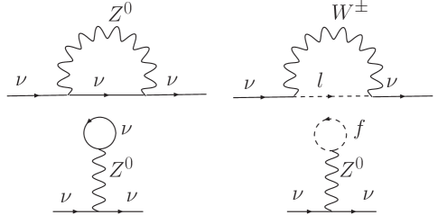
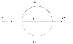
Figure 1: Left: one loop contributions to the self energy, the diagrams in the second line yield $\Sigma^{tad}$. These contributions are of $\mathcal{O}(G_{F})$. Right: two loops contribution of $\mathcal{O}(G^{2}_{F})$ to the self-energy in Fermi’s effective field theory limit, with internal lines corresponding to hadrons and the charged lepton, or alternatively quarks and the charged lepton above the QCD phase transition.

In a medium at temperature $T$ the real part of the one-loop contributions to $S(k,\omega)$ is of the form[47, 53, 14, 8]

$$S_{R}(k,\omega)=(\omega+k)\,G_{F}T^{3}\left[L+\frac{T}{M^{2}_{W}}\left(a\omega+bk\right)\right]$$ (60)

where $L$ is a function of the asymmetries of the fermionic species and $a,b$ simple coefficients, all of which may be read from the results in ref.[47, 8, 53]. Assuming that all asymmetries are of the same order as the baryon asymmetry in the early Universe $L\sim 10^{-9}$ the term $\propto T/M^{2}_{W}$ in (60) for $\omega\sim k\sim T$ dominates over the asymmetry term for $T\gtrsim 3\,\mathrm{MeV}$[47, 53] and in what follows we neglect the CP violating terms associated with the lepton asymmetry.

The imaginary part to one loop order is obtained from a Cutkosky cut (discontinuity) of the diagrams with vector boson exchange shown on the left side in figure (2) and is determined by the processes $W\rightarrow l_{a}\overline{\nu}_{a},Z\rightarrow\overline{\nu}_{a}\nu_{a}$. Both of these contributions are exponentially suppressed at temperatures $T\ll M_{W,Z}$, hence the one-loop contributions to the imaginary part of $S(k;\omega)$ is negligible for temperatures well below the electroweak scale. The two loop contribution to the imaginary part is obtained from the discontinuity cut of the two loop diagram with internal hadron or quark and charged lepton lines in figure (1). Some of the processes that contribute to the imaginary part in this order are for example neutron $\beta$ decay $n\rightarrow p+e^{+}+\overline{\nu}$ and its inverse, along with scattering processes in the medium. The imaginary part of the self-energy for these contributions on-shell is proportional to $G^{2}_{F}\,k\,T^{4}$[47, 14] at temperatures $T\ll M_{W}$. Therefore in this temperature range

$$S_{I}(k,\omega)\sim(\omega+k)\,G^{2}_{F}\,k\,T^{4}\,.$$ (61)

The consistency and validity of perturbation theory and of Fermi’s effective field theory for scales $\omega,k,T\ll M_{W}$ entail the following inequality

$$S_{I}(k,\omega)\ll S_{R}(k,\omega)\,.$$ (62)

For example near the neutrino mass shell for ultrarelativistic neutrinos with $\omega\sim k$, assuming $L\sim 10^{-9}$ and discarding this CP violating contribution for $T>3\,\mathrm{MeV}$ because it is subleading, we find

$$\frac{S_{I}(k,\omega)}{S_{R}(k,\omega)}\sim g^{2}$$ (63)

with $g$ the standard model weak coupling. This discussion is relevant for the detailed understanding when the quantum Zeno effect is operative (see section (4) below).

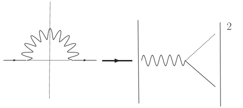
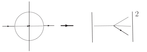
Figure 2: Contributions to the imaginary part of the self energy, the vertical line represents a Cutkosky cut. Left: discontinuity from the one loop contributions to the self energy of $\mathcal{O}(G_{F})$, from the decay of vector bosons for example $W\rightarrow l\overline{\nu}$. Right: discontinuity from the two loops contribution of $\mathcal{O}(G^{2}_{F})$, arising for example from $n\rightarrow p+e^{+}+\overline{\nu}_{e}$ or similar processes at the quark level.

The propagator $G(k;\omega)$ for negative helicity neutrinos is found to be given by

$$G(k;\omega)=\frac{1}{2\beta}\Bigg{[}\frac{1}{\alpha-\beta}-\frac{1}{\alpha+\beta}\Bigg{]}\,\left(\begin{array}[]{cc}\alpha+\beta\cos 2\theta_{m}&-\beta\sin 2\theta_{m}\\ -\beta\sin 2\theta_{m}&\alpha-\beta\cos 2\theta_{m}\\ \end{array}\right)\,,$$ (64)

where we have suppressed the arguments for economy of notation, and defined

$$\alpha = \omega^{2}-k^{2}-\overline{M}^{\,2}+\frac{1}{2}S_{R}(k,\omega)+\frac{i}{2}S_{I}(k,\omega)\,,$$ (65)

$$\beta = \frac{\delta M^{2}}{2}\Bigg{[}\Big{(}\cos 2\theta-\frac{S_{R}(k,\omega)}{\delta M^{2}}-i\frac{S_{I}(k,\omega)}{\delta M^{2}}\Big{)}^{2}+\sin^{2}2\theta\Bigg{]}^{\frac{1}{2}}\,,$$ (66)

$$\theta_{m} \equiv \theta^{(-1)}_{m}(k,s=-i\omega+\epsilon)\,.$$ (67)

The inequality (62) licenses us to write $\beta$ consistently up to $\mathcal{O}(G^{2}_{F})$ as

$$\beta\simeq\frac{\delta M^{2}}{2}\rho(k,\omega)-\frac{i}{2}S_{I}(k,\omega)\cos 2\theta_{m}\,,$$ (68)

where

$$\rho(k,\omega)=\Bigg{[}\Big{(}\cos 2\theta-\frac{S_{R}(k,\omega)}{\delta M^{2}}\Big{)}^{2}+\sin^{2}2\theta\Bigg{]}^{\frac{1}{2}}\,.$$ (69)

Equation (64) makes manifest that $G(k;\omega)$ is strongly peaked at the values of $\omega$ for which $\alpha=\pm\beta$. These determine the position of the complex poles in the analytic continuation. In the relativistic approximation $k\gg M_{1,2}$ we find:

• For $\alpha=\beta$:

  $$\omega_{1}(k)=E_{1}(k)-i\,\frac{\Gamma_{1}(k)}{2}$$ (70)

  with

  $$E_{1}(k) \approx k+\frac{1}{2k}\left[\overline{M}^{\,2}+\frac{\delta M^{2}}{2}\rho(k)-\frac{S_{R}(k)}{2}\right]$$ (71)

  $$\frac{\Gamma_{1}(k)}{2} = \frac{\Gamma_{aa}(k)}{2}\cos^{2}\theta_{m}(k)\,$$ (72)

• For $\alpha=-\beta$:

  $$\omega_{2}(k)=E_{2}(k)-i\frac{\Gamma_{2}(k)}{2}$$ (73)

  with

  $$E_{2}(k) \approx k+\frac{1}{2k}\left[\overline{M}^{\,2}-\frac{\delta M^{2}}{2}\rho(k)-\frac{S_{R}(k)}{2}\right]$$ (74)

  $$\frac{\Gamma_{2}(k)}{2} = \frac{\Gamma_{aa}(k)}{2}\sin^{2}\theta_{m}(k)\,.$$ (75)

where

$$\rho(k)\equiv\Bigg{[}\Big{(}\cos 2\theta-\frac{S_{R}(k,\omega=k)}{\delta M^{2}}\Big{)}^{2}+\sin^{2}2\theta\Bigg{]}^{\frac{1}{2}}\,,$$ (76)

and $\Gamma_{aa}(k)$ is the standard model result for the scattering rate of the active neutrino species[8, 47, 41, 42]

$$\frac{\Gamma_{aa}(k)}{2}=\frac{S_{I}(k,\omega=k)}{2k}=\frac{1}{4}\mathrm{Tr}(\gamma^{0}-\vec{\gamma}\cdot\hat{\textbf{ k}})\mathrm{Im}{\Sigma}_{aa}(\vec{k},\omega=k)\sim G^{2}_{F}\,T^{4}\,k$$ (77)

and $\theta_{m}(k)=\theta^{(h=-1)}_{m}(k,s=-ik)$ is the mixing angle in the medium for negative helicity neutrinos of energy $\omega\sim k$ in the relativistic limit. The relations (72,75) are the same as those recently found in reference[46].

Combining all the results we find

$$\left(\begin{array}[]{c}\nu_{a}(\vec{k},t)\\ \nu_{s}(\vec{k},t)\\ \end{array}\right) =\Bigg{[}e^{-iE_{1}(k)t}\,e^{-\frac{\Gamma_{1}(k)}{2}t}\,\frac{1}{2}\left(\begin{array}[]{cc}1+\cos 2\theta_{m}(k)&-\sin 2\theta_{m}(k)\\ -\sin 2\theta_{m}(k)&1-\cos 2\theta_{m}(k)\\ \end{array}\right)+$$ (87)

$$e^{-iE_{2}(k)t}\,e^{-\frac{\Gamma_{2}(k)}{2}\,t}\,\frac{1}{2}\left(\begin{array}[]{cc}1-\cos 2\theta_{m}(k)&\sin 2\theta_{m}(k)\\ \sin 2\theta_{m}(k)&1+\cos 2\theta_{m}(k)\\ \end{array}\right)\Bigg{]}\left(\begin{array}[]{c}\nu_{a}(\vec{k},0)\\ \nu_{s}(\vec{k},0)\\ \end{array}\right)$$

This expression can be written in the following more illuminating manner,

$$\left(\begin{array}[]{c}\nu_{a}(\vec{k},t)\\ \nu_{s}(\vec{k},t)\\ \end{array}\right)=U(\theta_{m}(k))\left(\begin{array}[]{cc}e^{-iE_{1}(k)t}\,e^{-\frac{\Gamma_{1}(k)}{2}t}&0\\ 0&e^{-iE_{2}(k)t}\,e^{-\frac{\Gamma_{2}(k)}{2}\,t}\\ \end{array}\right)U^{-1}(\theta_{m}(k))\left(\begin{array}[]{c}\nu_{a}(\vec{k},0)\\ \nu_{s}(\vec{k},0)\\ \end{array}\right)\,,$$ (88)

where $U(\theta_{m}(k))$ is the mixing matrix (12) but in terms of the mixing angle in the medium.

In obtaining the above expressions we have neglected perturbative corrections from wave function renormalization and replaced $\omega+k\sim 2k$ thus neglecting terms that are subleading in the relativistic limit, and the imaginary part in $\omega$, which although it is of $\mathcal{O}(G^{2}_{F})$, yields the effective Wigner-Weisskopf approximation[46].

2.4 Physical interpretation:

The above results have the following clear physical interpretation. The active (a) and sterile (s) neutrino fields in the medium are linear combinations of the fields associated with the $1,2$ quasiparticle modes with dispersion relations $E_{1,2}(k)$ and damping rates $\Gamma_{1,2}(k)$ respectively, on the mass shell of the quasiparticle modes the relation between them is the usual one for neutrinos propagating in a medium with an index of refraction, namely

$$\nu_{a}(\vec{k},t) = \cos\theta_{m}(k)~{}\nu_{1}(\vec{k},t)+\sin\theta_{m}(k)~{}\nu_{2}(\vec{k},t)$$ (89)

$$\nu_{s}(\vec{k},t) = \cos\theta_{m}(k)~{}\nu_{2}(\vec{k},t)-\sin\theta_{m}(k)~{}\nu_{1}(\vec{k},t)\,.$$ (90)

These relations between the expectation values of flavor fields and the fields associated with the propagating quasiparticle modes in the medium are obtained from the diagonalization of the neutrino propagator on the mass shell of the quasiparticle modes. These are recognized as the usual relations between flavor and “mass” fields in a medium with an index of refraction.

At temperatures much higher than that at which a resonance occurs (and for $k\sim T$) $\theta_{m}(k)\sim\pi/2$ then $\nu_{a}\sim\nu_{2}$, and the active neutrino features a damping rate $\Gamma_{2}\sim\Gamma_{aa}$ while the sterile neutrino $\nu_{s}\sim\nu_{1}$ with a damping rate $\Gamma_{1}=\Gamma_{aa}\cos^{2}\theta_{m}(k)\ll\Gamma_{aa}$. In the opposite limit for temperatures much lower than that of the resonance and for very small vacuum mixing angles $\nu_{a}\sim\nu_{1}$ and features a damping rate $\Gamma_{1}\sim\Gamma_{aa}$ while $\nu_{s}\sim\nu_{2}$ with a damping rate $\Gamma_{2}\sim\Gamma_{aa}\sin^{2}\theta\ll\Gamma_{aa}$. Thus it is clear that in both limits the active neutrino has the larger damping rate and the sterile one the smallest one. This physical interpretation confirms that there must be two widely different time scales for relaxation in the high and low temperature limits, the longest time scale or alternatively the smallest damping rate always corresponds to the sterile neutrino. This is obviously in agreement with the expectation that sterile neutrinos are much more weakly coupled to the plasma than the active neutrinos for $\sin 2\theta_{m}(k)\sim 0$. This analysis highlights that two time scales must be expected on physical grounds, not just one, the decoherence time scale, which only determines the suppression of the overlap between the propagating states in the mixed neutrino state.

The solution (87) can also be obtained from an effective Schroedinger-like equation but with an effective Weisskopf-Wigner Hamiltonian[46], not for the quantum states, which are not decaying, but for the ensemble averages,

$$i\frac{d}{dt}\left(\begin{array}[]{c}\nu_{a}(\vec{k},t)\\ \nu_{s}(\vec{k},t)\\ \end{array}\right)=\mathcal{H}_{ww}\left(\begin{array}[]{c}\nu_{a}(\vec{k},t)\\ \nu_{s}(\vec{k},t)\\ \end{array}\right)$$ (91)

where the Weisskopf-Wigner effective Hamiltonian is

$$\mathcal{H}_{ww}=\Big{(}k+\frac{\overline{M}^{2}}{2k}\Big{)}\mathbb{I}+\frac{\delta M^{2}}{4k}\left(\begin{array}[]{cc}\cos 2\theta&-\sin 2\theta\\ -\sin 2\theta&-\cos 2\theta\\ \end{array}\right)-\frac{1}{2k}\Big{(}S_{R}(k)+iS_{I}(k)\Big{)}\left(\begin{array}[]{cc}1&0\\ 0&0\\ \end{array}\right)\,.$$ (92)

Although this form of the time evolution looks similar to the usual quantum mechanical one, we emphasize that this equation of motion is for the ensemble averages of the neutrino operators and $S_{R,I}$ are obtained from the self-energy on the mass shell of ultrarelativistic neutrinos. This self energy is an ensemble average of correlation functions of the operators that describe the degrees of freedom in the medium. This time evolution is an a posteriori consequence of the field-theoretical analysis, which unambiguously reveals the time evolution. While the description afforded by the Schroedinger-like equation for the ensemble averages with a non-hermitian Weisskopf-Wigner Hamiltonian is simpler, it can only be rigorously justified through the detailed study presented above.

The emergence of two time scales can also be gleaned in the pioneering work on sterile neutrino production of ref.[40] (see eqn. (10) in that reference) which in this reference where obtained within a phenomenological Wigner-Weisskopf approximation akin to (91,92). Our quantum field theory study based on the full density matrix and the neutrino propagator in the medium provides a consistent and systematic treatment of propagation in the medium that displays both time scales and provides a derivation of the effective Schroedinger-like evolution with the Weisskopf-Wigner Hamiltonian[46].

3 Quantum Zeno effect

3.1 Real time interpretation and general conditions

Consider a density matrix in which the expectation value of the active neutrino field is non-vanishing, but that of the sterile neutrino field vanishes at the initial time $t=0$, namely $\nu_{a}(\vec{k},0)\neq 0~{};~{}\nu_{s}(\vec{k},0)=0$. Then it is clear from equation (87) that flavor off-diagonal density matrix elements develop in time signaling that sterile neutrinos are produced via active-sterile mixing with amplitude

$$\nu_{s}(\vec{k},t)=-\frac{1}{2}\sin 2\theta_{m}(k)\Bigg{[}e^{-iE_{1}(k)t}\,e^{-\frac{\Gamma_{1}(k)}{2}t}\,-e^{-iE_{2}(k)t}\,e^{-\frac{\Gamma_{2}(k)}{2}\,t}\Bigg{]}\nu_{a}(\vec{k},0)$$ (93)

From the solution (93) we introduce the generalized transition probability in the medium from the expectation values of the neutrino fields in the density matrix, these are the transition probabilities between ensemble averages of one-particle states of the neutrino fields,

$$P_{a\rightarrow s}(t)=\Bigg{|}\frac{\nu_{s}(\vec{k},t)}{\nu_{a}(\vec{k},0)}\Bigg{|}^{2}=\frac{\sin^{2}2\theta_{m}(k)}{2}\,e^{-\Gamma(k)t}\,\Bigg{[}\cosh(\gamma(k)t)-\cos(\Delta E(k)t)\Bigg{]}$$ (94)

where

$$\Gamma(k) = \frac{1}{2}\Big{(}\Gamma_{1}(k)+\Gamma_{2}(k)\Big{)}=\frac{\Gamma_{aa}(k)}{2}$$ (95)

$$\gamma(k) = \frac{1}{2}\Big{(}\Gamma_{1}(k)-\Gamma_{2}(k)\Big{)}=\frac{\Gamma_{aa}(k)}{2}\cos 2\theta_{m}(k)$$ (96)

$$\Delta E(k) = E_{1}(k)-E_{2}(k)=\frac{\delta M^{2}}{2\,k}\rho(k)$$ (97)

For the analysis that follows it is more convenient to write (94) in the form

$$P_{a\rightarrow s}(k;t)=\frac{\sin^{2}2\theta_{m}(k)}{4}\,\Bigg{[}{e^{-\Gamma_{1}(k)\,t}}+{e^{-\Gamma_{2}(k)\,t}}\,-2\,e^{-\Gamma(k)t}\cos(\Delta E(k)t)\Bigg{]}\,.$$ (98)

The first two terms are obviously the probabilities for the quasiparticle modes $1,2$, while the oscillatory term is the usual interference between these but now damped by the factor $e^{-\Gamma(k)t}$. This form of the transition probability is remarkably similar to the familiar transition probability in $K_{0}-\overline{K}_{0}$ or $B_{0}-\overline{B}_{0}$ oscillations[60, 61]. However we emphasize that (98) is the generalized transition probability extracted from expectation values in the density matrix.

We highlight that the decoherence time scale is precisely $\Gamma^{-1}(k)=2/\Gamma_{aa}(k)$ as anticipated in references[34, 41], since the interference between the two quasiparticle modes is suppressed on this time scale. However, the total transition probability is suppressed on this time scale only if $\Gamma_{1}=\Gamma_{2}=\Gamma$, namely near a resonance. In this case

$$P_{a\rightarrow s}(t)=\sin^{2}2\theta_{m}~{}e^{-\frac{\Gamma_{aa}}{2}\,t}\,\sin^{2}\left[\frac{\Delta E}{2}\,t\right]\,,$$ (99)

which is the result quoted in reference[41] (see eqn. (4)). Under these conditions quantum Zeno suppression occurs when $\Gamma(k)\gg\Delta E(k)$ in which case the decoherence time scale is much smaller than the oscillation time scale and the transition probability is suppressed before $a\rightarrow s$ oscillations take place.

However, far away on either side of the resonance, although the oscillatory interference term is suppressed on the decoherence time scale $\Gamma^{-1}$, the transition probability is not suppressed on this scale but on a much longer time scale, determined by the smaller of $\Gamma_{1,2}$. Only when $\Gamma_{1}=\Gamma_{2}=\Gamma$, namely $\gamma=0$ both the coherence (oscillatory interference term) and the transition probability are suppressed on the decoherence time scale. This phenomenon is displayed in figures (3,4 ) which show the transition probability as a function of time without the prefactor $\sin^{2}2\theta_{m}(k)$ for several values of the ratios $\gamma/\Gamma;\Delta E/\Gamma$.

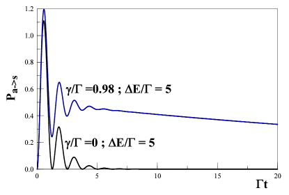
Figure 3: The transition probability $P_{a\rightarrow s}(t)$ (without the prefactor $\sin^{2}2\theta_{m}/2$) vs. $\Gamma t$. The figure depicts the cases $\cos 2\theta_{m}(k)=0.98$ and $\cos 2\theta_{m}(k)=0$ respectively, both with $\Delta E/\Gamma=\delta M^{2}\rho(k)/2k\Gamma=5$. The scale for suppression of the oscillatory interference is $1/\Gamma$ in both cases.

Even for $\Gamma(k)\gg\Delta E(k)$, claimed in the literature [34, 8] to be the condition for quantum Zeno suppression, the transition probability is substantial on time scales much longer than $\Gamma^{-1}$ if $\Gamma_{1}$ and $\Gamma_{2}$ are widely separated, namely if $|\gamma/\Gamma|\sim 1$. This situation is depicted in figure (5). From this analysis we conclude that the conditions for quantum Zeno suppression of $P_{a\rightarrow s}(t)$ are: i): $\Gamma(k)\gg\Delta E(k)$ and ii):) $\gamma(k)\sim 0$, namely $\Gamma_{1}(k)\sim\Gamma_{2}(k)$. These conditions are obtained directly from the time dependence of $P_{a\rightarrow s}(t)$ without taking any time average. We then emphasize that it is not necessary to average the probability over time to recognize the criteria for the quantum Zeno effect, these can be directly gleaned from the time evolution of the probability as originally proposed[33].

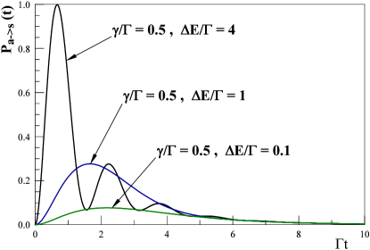
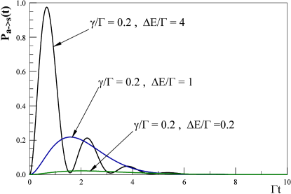
Figure 4: The transition probability $P_{a\rightarrow s}(t)$ (without the prefactor $\sin^{2}2\theta_{m}/2$) vs. $\Gamma t$. The left panel is for $\gamma/\Gamma=0.5$, $\Delta E/\Gamma=4,1,0.1$, the right panel is for $\gamma/\Gamma=0.2$, $\Delta E/\Gamma=4,1,0.2$.

Figure 5: The transition probability $P_{a\rightarrow s}(t)$ (without the prefactor $\sin^{2}2\theta_{m}/2$) vs. $\Gamma t$ in the quantum Zeno limit $\Gamma\gg\Delta E$ for the cases $\cos 2\theta_{m}(k)=0.98,0$ and $\Delta E/\Gamma=\delta M^{2}\rho(k)/2k\Gamma=0.1$. The ramp-up time scale is $\sim 1/\Gamma_{1}\sim 1/\Gamma$. In the left figure the damping time scale is $\sim 1/\Gamma_{2}\sim 50/\Gamma$. The right figure displays the resonant case for which the damping and coherence time scale coincide, when the conditions for quantum Zeno suppression are fulfilled.

From the arguments in reference[41], the effective sterile neutrino production rate is obtained from the average of the transition probability on the decoherence time scale $\tau_{dec}$. Using the result (98) we find instead

$$\Big{\langle}P_{a\rightarrow s}\Big{\rangle}\equiv{\Gamma}\int^{\infty}_{0}P_{a\rightarrow s}(t)\,dt=\frac{\sin^{2}2\theta_{m}}{2}~{}\frac{\left(\frac{\gamma}{{\Gamma}}\right)^{2}+\left(\frac{\Delta E}{{\Gamma}}\right)^{2}}{\left[1-\left(\frac{\gamma}{{\Gamma}}\right)^{2}\right]\left[1+\left(\frac{\Delta E}{{\Gamma}}\right)^{2}\right]}\,,$$ (100)

where $\Gamma,\gamma$ are given by eqns. (95,96) respectively.

This expression features two remarkable differences with the result (5)[41]: the extra terms $(\gamma/\Gamma)^{2}$ in the numerator and $1-(\gamma/\Gamma)^{2}$ in the denominator, both are consequence of the fact that the relaxation is determined by two time scales $\Gamma_{1},\Gamma_{2}$. Only when these scales are equal, namely when $\gamma=0$ the result (5) often used in the literature is recovered.

We note that the result (100) is not singular since $1-(\gamma^{2}/\Gamma^{2})=\sin^{2}2\theta_{m}$, (see also the discussion in section (4.1)).

This analysis leads us to state that the complete conditions for quantum Zeno suppression of the transition probability are that both $\gamma/\Gamma\ll 1$ and $\Delta E/\Gamma\ll 1$. That these are indeed the correct necessary conditions for quantum Zeno suppression can be gleaned from figures (4, 5) which display the transition probability (without the prefactor $\sin^{2}2\theta_{m}/2$) as a function of time for several values of the ratios $\gamma/\Gamma,\Delta E/\Gamma$ without performing the time average.

3.2 High and low temperature limits: assessment of the quantum Zeno condition

In order to establish when the quantum Zeno condition $\Delta E(k)/\Gamma_{aa}(k)\ll 1$ is fulfilled we focus on the cases far away from resonances and, according to the exhaustive analysis of ref.[5, 8] and the constraints from the X-ray background in clusters[29, 30], in the region of parameter space $1\,\mathrm{keV}\lesssim m_{s}\lesssim 10\,\mathrm{keV}$ , $10^{-10}\lesssim\sin^{2}2\theta\lesssim 10^{-6}$. We consider $T\gtrsim 3\,\textrm{MeV}$ for which we can neglect the CP violating asymmetry contribution in (60) assuming that it is of the same order as the baryon asymmetry $L\sim 10^{-9}$[47, 53]. In this regime $\delta M^{2}\sim m^{2}_{s}$, and from (60) we find

$$\frac{S_{R}(k,k)}{\delta M^{2}}\sim 10^{-14}\,\Bigg{(}\frac{T}{\textrm{MeV}}\Bigg{)}^{6}\,\Bigg{(}\frac{k}{T}\Bigg{)}^{2}\,\Bigg{(}\frac{\textrm{keV}}{m_{s}}\Bigg{)}^{2}$$ (101)

Taking $k\sim T$ and $m_{s}\sim 1\,\textrm{keV}$ the MSW resonance $S_{R}(k,k)/\delta M^{2}=1$ occurs at $T_{MSW}\sim 215\,\textrm{MeV}$ (a more precise estimate yields $T\sim 180\,\textrm{MeV}$[5, 8]). For $T\gg T_{MSW}$ corresponding to $S_{R}(k,k)/\delta M^{2}\gg 1$ the active sterile oscillation frequency becomes

$$\Delta E(k)=\frac{\delta M^{2}}{2\,k}\rho(k)\sim\frac{S_{R}(k,k)}{2k}\sim\frac{G_{F}\,T^{4}\,k}{M^{2}_{W}}$$ (102)

From the result (77) for $\Gamma_{aa}(k)$ we find in the high temperature limit $T\gg T_{MSW}$

$$\frac{2\,\Delta E(k)}{\Gamma_{aa}(k)}\sim\frac{G_{F}\,T^{4}\,k}{G^{2}_{F}\,T^{4}\,k\,M^{2}_{W}}\sim\frac{1}{g^{2}}\gg 1$$ (103)

where $g$ is the weak coupling. We note that in the high temperature limit the ratio $\Delta E(k)/\Gamma_{aa}(k)$ becomes independent of $T,k$. This result is in agreement with the conclusions in ref.[48].

In the low temperature limit $3\,\textrm{MeV}\lesssim T\ll T_{MSW}$ it follows that $S_{R}(k,k)/\delta M^{2}\ll 1$ and the active-sterile oscillation frequency is

$$\Delta E(k)\sim\frac{m^{2}_{s}}{2k}$$ (104)

hence the ratio

$$\frac{\Delta E(k)}{\Gamma_{aa}(k)}\sim\frac{m^{2}_{s}}{G^{2}_{F}\,T^{4}\,k^{2}}\sim 10^{16}\,\Bigg{(}\frac{m_{s}}{\textrm{keV}}\Bigg{)}^{2}\,\Bigg{(}\frac{T}{\textrm{MeV}}\Bigg{)}^{-6}\,\Bigg{(}\frac{k}{T}\Bigg{)}^{-2}$$ (105)

which for $k\sim T$ can be simplified to

$$\frac{2\,\Delta E(k)}{\Gamma_{aa}(k)}\sim 10^{2}\Bigg{(}\frac{T_{MSW}}{T}\Bigg{)}^{6}\gg 1\,.$$ (106)

At the MSW resonance $T=T_{MSW}$, $\cos 2\theta_{m}\sim 0$, $\Delta E(k)=m^{2}_{s}\sin 2\theta/2k$ and the ratio becomes

$$\frac{2\,\Delta E(k)}{\Gamma_{aa}(k)}\sim 10^{2}\sin 2\theta\ll 1$$ (107)

for $10^{-5}\lesssim\sin 2\theta\lesssim 10^{-3}$. Therefore at the MSW resonance $\cos 2\theta_{m}(k)\sim 0$ and both conditions for quantum Zeno suppression, $\gamma/\Gamma\ll 1$ , $\Delta E/\Gamma\ll 1$ are fulfilled. However, we point out that near the resonance the oscillation frequency becomes $\Delta E\sim\frac{\delta M^{2}}{2k}|\sin\theta|$ only if the second order corrections to the dispersion relations (real part of the poles) are neglected, therefore if $\Gamma\gg\Delta E$ a reassessment of the perturbative expansion including second order corrections to the dispersion relations is required, since $\Gamma\propto G^{2}_{F}$. Therefore this analysis leads us to unambiguously conclude that with standard model interactions for the active neutrino quantum Zeno suppression is not realizable either at high temperatures, when the matter potential dominates or at very low temperatures where the mixing angle is close to the vacuum value. Such possibility may only emerge very near an MSW resonance, however for small mixing angle this case requires a thorough reassessment of the dispersion relations in the medium including corrections of $\mathcal{O}(G^{2}_{F})$ to the oscillation frequency.

3.3 Validity of the perturbative expansion:

The quantum Zeno condition $\Gamma_{aa}(k)\gg\Delta E(k)$ requires a consistent assessment of the validity of the perturbative expansion in the standard model and or Fermi’s effective field theory. The active neutrino scattering rate $\Gamma_{aa}\propto G^{2}_{F}\,k\,T^{4}$ is a two loops result, while to leading order in weak interactions, the index of refraction contribution to the dispersion relation $S_{R}(k,\omega)$ is of one-loop order[47, 53]. In the high temperature limit when $S_{R}\gg\delta M^{2}\sim m^{2}_{s}$ the active-sterile oscillation frequency is

$$\Delta E(k)\sim\frac{|S_{R}(k,k)|}{2k}$$ (108)

combining this result with equation (77) at high temperature or density where the index of refraction dominates over $\delta M^{2}$, it follows that

$$\frac{\Delta E(k)}{\Gamma_{aa}(k)}\sim\frac{|S_{R}(k,k)|}{S_{I}(k,k)}$$ (109)

for $k\sim T$ the perturbative relation (63) states that this ratio is $\gtrsim 1/g^{2}\gg 1$ where $g$ is the weak gauge coupling. An opposite ratio, namely $\Delta E(k)/\Gamma_{aa}\ll 1$ would entail that the two-loop contribution ($\Gamma_{aa}$) is larger than the one-loop contribution that yields the index of refraction $S_{R}$. Thus quantum Zeno suppression at high temperature when the index of refraction dominates the oscillation frequency necessarily implies a breakdown of the strict perturbative expansion. Such potential breakdown of perturbation theory in the standard model or Fermi’s effective field theory in the quantum Zeno limit has been already observed in a different context by these authors in ref.[48], and deserves deeper scrutiny. We are currently exploring extensions beyond the standard model in which neutrinos couple to scalar fields motivated by Majoron models, in these extensions the coupling to the scalar (Majoron) provides a different scale that permits to circumvent this potential caveat. We expect to report on our results in a forthcoming article[62].

4 Implications for sterile neutrino production in the early Universe:

4.1 Time averaged transition probability, production rate and shortcomings of the rate equation

The effective sterile production rate proposed in ref.[41] and given by eqn. (2) requires the average of the transition probability $P_{a\rightarrow s}(t)$ over the decoherence time scale. Hence, combining (3) with the transition probability in the medium (94,95,96) yields the following time averaged transition probability (compare to eqn. (100))

$$\Big{\langle}P_{a\rightarrow s}\Big{\rangle}=\frac{\sin^{2}2\theta_{m}(k)}{2}~{}~{}\frac{\cos^{2}2\theta_{m}(k)+\Big{(}\frac{2\Delta E(k)}{\Gamma_{aa}(k)}\Big{)}^{2}}{\sin^{2}2\theta_{m}(k)\Bigg{[}1+\Big{(}\frac{2\Delta E(k)}{\Gamma_{aa}(k)}\Big{)}^{2}\Bigg{]}}$$ (110)

We have purposely kept the $\sin^{2}2\theta_{m}(k)$ in the numerator and denominator to highlight the cancelation between this factor arising from the transition probability in the numerator with the factor $1-(\gamma/\Gamma)^{2}$ arising from the total integrated probability in the denominator. The factor $\cos^{2}2\theta_{m}(k)$ in the numerator and the $\sin^{2}2\theta_{m}(k)$ in the denominator are hallmarks of the presence of the two different relaxation rates $\Gamma_{1}(k),\Gamma_{2}(k)$, and are responsible for the difference with the result (5). The extra factor $\sin^{2}2\theta_{m}(k)$ in the denominator signals an enhancement when $\theta_{m}(k)=0,\pi/2$. In the case $\theta_{m}(k)\sim 0$ the relaxation rate $\Gamma_{2}(k)\ll\Gamma_{1}(k)$ whereas for $\theta_{m}(k)\sim\pi/2$ the opposite holds, $\Gamma_{1}(k)\ll\Gamma_{2}(k)$. In either case there is a wide separation between the relaxation rates of the propagating modes in the medium and the longest time scale for relaxation dominates the time integral in (110). This is depicted in fig. (5).

This is an important difference with the result in [41] wherein it was assumed that $\Gamma_{1}=\Gamma_{2}$, in which case $\gamma=0$. For $\theta_{m}(k)\sim 0,\pi/2$, the ratio $\gamma/\Gamma\sim 1$ leads to an enhancement of the time averaged transition probability. The interpretation of this result should be clear. The probability $P_{a\rightarrow s}(t)$ has two distinct contributions, the interference oscillatory term, and the non-oscillatory terms. When one of these non-oscillatory terms features a much longer relaxation time scale, it dominates the integrand at long time after the interference term has become negligible, as shown in figure (5). Therefore the time integral receives the largest contribution from the term with the smallest relaxation rate, this is the origin of the factor $1-(\gamma/\Gamma)^{2}=\sin^{2}2\theta_{m}(k)$ in the denominator.

Taking the kinetic equation that describes sterile neutrino production (1) along with the effective production rate (2) at face value, the new result (110) for the average transition probability yields the effective production rate

$$\Gamma(a\rightarrow s;k)=\frac{\Gamma_{aa}(k)}{4}\,\frac{\cos^{2}2\theta_{m}(k)+\Big{(}\frac{2\Delta E(k)}{\Gamma_{aa}(k)}\Big{)}^{2}}{\Bigg{[}1+\Big{(}\frac{2\Delta E(k)}{\Gamma_{aa}(k)}\Big{)}^{2}\Bigg{]}}\,.$$ (111)

The result of references[41, 42, 8] is retrieved only near an MSW resonance for which $\cos 2\theta_{m}(k)\approx 0$, in this case the relaxation rates become the same and $\gamma=0$. However, accounting for both relaxation rates $\Gamma_{1};\Gamma_{2}$ yields the new result (110,111) which is generally very different from the usual one (5).

The result (111) is in clear contradiction with the analysis in section (2.4) wherein the physical interpretation of the damping rates identify the sterile degrees of freedom as very weakly coupled to the plasma both at high temperature ($\theta_{m}\sim\pi/2$) and low temperature ($\theta_{m}\sim 0$), therefore should feature small production rates. Contrary to this expectation, taking the limit of $\sin 2\theta_{m}(k)\sim 0$ in (111), still yields a non-vanishing sterile neutrino production rate despite the fact sterile neutrinos decouple from the plasma in this limit. The origin of this puzzling result is the time averaged probability $\langle P_{a\rightarrow s}\rangle$ (3) and not any ambiguity in the calculation of the relaxation rates or in the time dependence of the transition probability $P_{a\rightarrow s}(t)$. The time integral in the averaged expression (3) introduces a denominator $\sin^{2}2\theta_{m}(k)$ from the longest time scale, and it is this denominator that is responsible for the enhancement. Thus the unreliability of the result (111) is a direct consequence of using the time-averaged transition probability (3) in the rate equation (1).

The real time analysis presented above clearly suggests that far away from an MSW resonance when $\Gamma_{1}$ and $\Gamma_{2}$ differ widely, $\Gamma^{-1}$ is not the relevant time scale for suppression of the transition probability, but the longest of $\Gamma^{-1}_{1}$ and $\Gamma^{-1}_{2}$ therefore the time averaged transition probability (3) cannot be the correct ingredient in the rate equation. A more suitable definition of the average transition probability under these circumstances should be

$$\langle P_{a\rightarrow s}\rangle=\Gamma_{sm}\,\int^{\infty}_{0}P_{a\rightarrow s}(t)dt$$ (112)

where $\Gamma_{sm}$ is the smallest of $\Gamma_{1,2}$. In a non-expanding cosmology this would indeed be the correct definition of an average transition probability, however in the early Universe as the temperature diminishes upon cosmological expansion, $\Gamma_{sm}$ changes with time crossing from $\Gamma_{1}$ over to $\Gamma_{2}$ at the resonance and the alternative definition (112) would imply a “rate” with a sliding averaging time scale that changes rapidly near an MSW resonance. One can instead provide yet another suitable definition of an averaged transition rate

$$\langle P_{a\rightarrow s}\rangle=\frac{\Gamma_{1}\,\Gamma_{2}}{\Gamma_{1}+\Gamma_{2}}\,\int^{\infty}_{0}P_{a\rightarrow s}(t)dt\,.$$ (113)

When the two rates differ widely the prefactor always approximates the smaller one. Since

$$\frac{\Gamma_{1}\,\Gamma_{2}}{\Gamma_{1}+\Gamma_{2}}=\frac{\Gamma_{aa}}{4}\left[1-\frac{\gamma^{2}(k)}{\Gamma^{2}(k)}\right]$$ (114)

this definition would cancel the enhancement from the $\sin^{2}2\theta_{m}(k)$ in the denominator in (110) (still leaving the $\cos^{2}2\theta_{m}(k)$ in the numerator), but it misses the correct definition of the average rate by a factor $2$, namely by $100\%$, in the region of the resonance where $\Gamma_{1}=\Gamma_{2}=\Gamma_{aa}/2$.

Obviously the ambiguity in properly defining a time averaged transition probability stems from the wide separation of the time scales associated with the damping of the quasiparticle modes, far away from an MSW resonance. Near the resonance both time scales become comparable and there is no ambiguity in the averaging scale. Complicating this issue further is the fact that in the early Universe these time scales are themselves time dependent as a consequence of the cosmological expansion and feature a rapid crossover behavior at an MSW resonance.

4.2 Caveats of the kinetic description.

It is important to highlight the main three different aspects at the origin of the enhanced production rate given by equation (111) in the high temperature regime, for $\theta_{m}(k)\sim\pi/2$: i) the assumption of the validity of the usual rate equation in terms of a time-averaged transition probability wherein the relevant time scale for averaging is the decoherence time scale $1/\Gamma$, ii) the result of a complete self-energy calculation that yields two time scales which are widely different far away from an MSW resonance, in particular at very high and very low temperatures, iii) the generalized transition probability in the medium (98) obtained from expectation values in the full density matrix, rather than the usual quantum mechanical expression in terms of single particle states. The real time study of the transition probability shows that the oscillatory interference term is suppressed on the decoherence time scale $1/\Gamma$, but also that this is not the relevant time scale for the suppression of the transition probability far away from an MSW resonance. The transition probability actually grows during $1/\Gamma$ reaches its maximum on this time scale and remains near this value for a long time interval between $1/\Gamma$ and $1/\Gamma_{sm}$ where $\Gamma_{sm}$ is the smaller of $\Gamma_{1},\Gamma_{2}$. The enhanced rate emerges when taking for granted the definition of the time-averaged probability in terms of the decoherence scale but including in this expression the correct form of the transition probability (98). As discussed above, alternative definitions of a time-averaged rate could be given, but all of them have caveats when applied to sterile neutrino production in the early Universe.

However, we emphasize, that the underlying physical reason for the enhancement does not call for a simple redefinition of the rate but for a full reassessment of the kinetic equation of sterile neutrino production. The important fact is that the wide separation of scales prevent a consistent description in terms of a simple rate in the kinetic equation, a rate implies only one relevant time scale for the build-up or relaxation of population, whereas our analysis reveals two widely different scales that are of the same order only near an MSW resonance.

Kinetic rate equations are generally a Markovian limit of more complicated equations in which the transition probability in general features a non-linear time dependence . Only when the non-linear aspects of the time dependence of the transition probability are transients that disappear faster than the scale of build-up or relaxation an average transition probability per unit time, namely a rate, can be defined and the memory aspects associated with the time evolution of the transition probability can be neglected. This is not the case if there is a wide separation of scales, and under these circumstances the assumptions leading to the kinetic equation (1) must be revised and its validity questioned, very likely requiring a reassessment of the kinetic description. This situation becomes even more pressing in the early Universe. In the derivation of the average probability in ref.[41] the rate $\Gamma_{aa}$ (denoted by $\tau_{0}$ in that reference) is taken as a constant in the time integral in the average. This is a suitable approximation if the integrand falls off in the time scale $1/\Gamma_{aa}$, since this time scale is shorter than the Hubble expansion time scale for $T>1\,\textrm{MeV}$. However, if there is a much longer time scale, when one of the relaxation rates is very small, as is the case depicted in fig.(5), then this approximation cannot be justified and a full time-dependent kinetic description beyond a simple rate equation must be sought.

Thus we are led to conclude that the simple rate equation (1) based on the time-averaged transition probability (3) is likely incorrect far away from MSW resonances.

An alternative kinetic description based on a production rate obtained from quantum field theory has recently been offered[44] and seems to yield a result very different for the rate equation (1) in terms of the time-averaged transition probability. However, this alternative description focuses on the hadronic contribution near the MSW resonance, and as such cannot yet address the issue of the widely separated time scales far away from it. A full quantum field theoretical treatment far away from an MSW resonance which systematically and consistently treats the two widely different time scales is not yet available.

Thus we conclude that while the result for the rate (111) is a direct consequence of including the correct transition probability $P_{a\rightarrow s}(t)$ given by (98) into the rate equation (1), our field theoretical analysis of the full neutrino propagator in the medium, and the real time evolution of the transition probability, extracted from the full density matrix leads us to challenge the validity of the simple rate equation (1) with (2) to describe sterile neutrino production in the early Universe away from an MSW resonance.

5 Conclusions:

Motivated by the cosmological importance of sterile neutrinos, we reconsider an important aspect of the kinetics of sterile neutrino production via active-sterile oscillations at high temperature: quantum Zeno suppression of the sterile neutrino production rate.

Within an often used kinetic approach to sterile neutrino production, the production rate involves two ingredients: the active neutrino scattering rate $\Gamma_{aa}$ and a time averaged active-sterile transition probability $\langle P_{a\rightarrow s}\rangle$[39, 40, 41, 42, 8] in the case of one sterile and one active neutrino.

Unlike the usual treatment in terms of a truncated $2\times 2$ density matrix for flavor degrees of freedom, we study the dynamics of active-sterile transitions directly from the full real time evolution of the quantum field density matrix. Active-sterile transitions are studied as an initial value problem wherein the main ingredient is the full neutrino propagator in the medium, obtained directly from the quantum density matrix and includes the self-energy up to $\mathcal{O}(G^{2}_{F})$. The correct dispersion relations and damping rates of the quasiparticles modes are obtained from the neutrino propagator in the medium. We introduce a generalization of the active-sterile transition probability from the expectation values of the neutrino field operators in the density matrix.

There are three main results from our study:

• I): The damping rates of the two different propagating modes in the medium are given by

  $$\Gamma_{1}(k)=\Gamma_{aa}(k)\cos^{2}\theta_{m}(k)\,;\,\Gamma_{2}(k)=\Gamma_{aa}(k)\sin^{2}\theta_{m}(k)$$ (115)

  where $\Gamma_{aa}(k)\propto G^{2}_{F}\,k\,T^{4}$ is the active neutrino scattering rate and $\theta_{m}(k)$ is the mixing angle in the medium. The dispersion relations are the usual ones with the index of refraction correction[47], plus perturbatively small two-loop corrections of $\mathcal{O}(G^{2}_{F})$. We give a simple physical explanation for this result: for very high temperature when $\theta_{m}\sim\pi/2$, $\nu_{a}\sim\nu_{2};\nu_{s}\sim\nu_{1}$ and $\Gamma_{2}\sim\Gamma_{aa};\Gamma_{1}\ll\Gamma_{aa}$. In the opposite limit of very low temperature and small vacuum mixing angle $\theta_{m}\sim 0$ , $\nu_{a}\sim\nu_{1};\nu_{s}\sim\nu_{2}$ and $\Gamma_{1}\sim\Gamma_{aa};\Gamma_{2}\ll\Gamma_{aa}$. Thus in either case the sterile neutrino is much more weakly coupled to the plasma than the active one.

• II): We study the active-sterile transition probability $P_{a\rightarrow s}(t)$ directly in real time from the time evolution of expectation values of the neutrino field operators in the density matrix. The result is given by

  $$P_{a\rightarrow s}(k;t)=\frac{\sin^{2}2\theta_{m}(k)}{4}\,\Bigg{[}{e^{-\Gamma_{1}(k)\,t}}+{e^{-\Gamma_{2}(k)\,t}}\,-2\,e^{-\frac{1}{2}(\Gamma_{1}(k)+\Gamma_{2}(k))t}\cos(\Delta E(k)t)\Bigg{]}\,.$$ (116)

  The real time analysis shows that even when $\Gamma(k)\gg\Delta E(k)$, which in the literature [34, 8] is taken to indicate quantum Zeno suppression, the transition probability is substantial on time scales much longer than $\Gamma^{-1}$ if $\Gamma_{1}$ and $\Gamma_{2}$ are widely separated. While the oscillatory interference term is suppressed by the decoherence time scale $1/\Gamma(k)=2/\Gamma_{aa}(k)$ in agreement with the results of [34, 41], at very high or low temperature this is not the relevant time scale for the suppression of the transition probability, which is given by $1/\Gamma_{sm}$ with $\Gamma_{sm}$ the smaller between $\Gamma_{1},\Gamma_{2}$. We obtain the complete conditions for quantum Zeno suppression: i) $2\Delta E(k)/\Gamma_{aa}\ll 1$ where $\Delta E(k)$ is the oscillation frequency in the medium, and ii) $\Gamma_{1}\sim\Gamma_{2}$. This latter condition is only achieved near an MSW resonance. Furthermore we studied consistently up to second order in standard model weak interactions, in which temperature regime the quantum Zeno condition $\Gamma_{aa}(k)\gg\Delta E(k)$ is fulfilled. We find that for $m_{s}\sim\textrm{keV}$ and $10^{-5}\lesssim\sin 2\theta\lesssim 10^{-3}$[5, 8, 42] the opposite condition, $\Gamma_{aa}(k)\ll\Delta E(k)$ is fulfilled in the high temperature limit $T\gg T_{MSW}\sim 215\,\textrm{MeV}$, as well as in the low temperature regime $3\,\textrm{MeV}\lesssim T\ll T_{MSW}$. We therefore conclude that the quantum Zeno conditions are may only be fulfilled near an MSW resonance for $T\sim T_{MSW}$ but a firmer assessment of this possibility requires to include the $\mathcal{O}(G^{2}_{F})$ corrections to the index of refraction.

• III): Inserting the result (116) into the expressions for the time averaged transition probability (3) and the sterile neutrino production rate (2) yields an expression for this rate that is enhanced at very high or low temperature given by equation (111) instead of the result (5) often used in the literature. The surprising enhancement at high or low temperature implied by (111) originates in two distinct aspects: i) the assumption of the validity of the rate kinetic equation in terms of a time-averaged transition probability with an averaging time scale determined by the decoherence scale $2/\Gamma_{aa}$, and ii) inserting the result (116) into the definition of the time-averaged transition probability. The enhancement is a distinct result of the fact that at very high or low temperatures the decoherence time scale is not the relevant scale for suppression of $P_{a\rightarrow s}$ but either $1/\Gamma_{1}$ or $1/\Gamma_{2}$ whichever is longer in the appropriate temperature regime. Our analysis shows that far away from the region of MSW resonance, the transition probability reaches its maximum on time scale $1/\Gamma(k)$, remains near this value during a long time scale $1/\Gamma_{sm}\gg 1/\Gamma$. We have also argued that in the early Universe the definition of a time averaged transition probability is ambiguous far away from MSW resonances. Our analysis leads us to conclude that the simple rate equation (1) in terms of the production rate (2), ( 3) is likely incorrect far away from MSW resonances.

We emphasize and clarify an important distinction between the results summarized above. Whereas ${\bf I}$ and ${\bf II}$ are solidly based on a consistent and systematic quantum field theory calculation of the neutrino propagator, the correct equations of motion for the quasiparticle modes in the medium and the time evolution of expectation values of neutrino field operators in the quantum density matrix, the results summarized in ${\bf III}$ are a consequence of the assumption on the validity of the kinetic description based on the simple rate equation (1) with an effective rate (2) in terms of the time-averaged transition probability (3). The enhancement of the sterile production rate arising from this assumption, along with the ambiguity in properly defining a time-averaged transition probability in an expanding cosmology in the temperature regime far away from a MSW resonance all but suggest important caveats in the validity of the kinetic description for sterile neutrino production in terms of a simple rate equation in this regime. Our analysis suggests that a deeper understanding of possible quantum Zeno suppression at high temperature requires a reassessment of the validity of the perturbative expansion in the standard model or in Fermi’s effective field theory. Further studies of these issues are in progress.

- [1] C. W. Kim and A. Pevsner, Neutrinos in Physics and Astrophysics, (Harwood Academic Publishers, USA, 1993).
- [2] R. N. Mohapatra and P. B. Pal, Massive Neutrinos in Physics and Astrophysics, (World Scientific, Singapore, 2004).
- [3] M. Fukugita and T. Yanagida, Physics of Neutrinos and Applications to Astrophysics, (Springer-Verlag Berlin Heidelberg 2003).
- [4] G. G. Raffelt, Stars as Laboratories for Fundamental Physics, (The University of Chicago Press, Chicago, 1996); astro-ph/0302589; New Astron.Rev. 46, 699 (2002); hep-ph/0208024.
- [5] S. Dodelson and L. M. Widrow, Phys. Rev. Lett. 72, 17 (1994).
- [6] T. Asaka, M. Shaposhnikov, A. Kusenko, Phys. Lett. B 638, 401 (2006).
- [7] X. Shi, G. M. Fuller, Phys. Rev. Lett. 83, 3120 (1999).
- [8] K. Abazajian, G. M. Fuller, M. Patel, Phys. Rev. D64, 023501 (2001).
- [9] A. D. Dolgov and S. H. Hansen, Astropart. Phys. 16, 339 (2002).
- [10] K. Abazajian, G. M. Fuller, Phys. Rev. D66, 023526 (2002).
- [11] K. Abazajian, Phys. Rev. D73, 063506 (2006), ibid, 063513 (2006).
- [12] P. Biermann, A. Kusenko, Phys. Rev. Lett. 96, 091301 (2006).
- [13] K. Abazajian, S. M. Koushiappas, Phys. Rev. D74 023527 (2006).
- [14] A. D. Dolgov, Phys. Rept. 370, 333 (2002); Surveys High Energ.Phys. 17 91 (2002).
- [15] J. Lesgourgues, S. Pastor, Phys.Rept. 429 307, (2006).
- [16] G. Raffelt, G. Sigl, Astropart.Phys. 1, 165 (1993).
- [17] S. Hannestad, hep-ph/0602058.
- [18] P. L. Biermann, F.l Munyaneza,astro-ph/0609388; astro-ph/0702164;astro-ph/0702173;
- [19] J. Hidaka, G. M. Fuller, astro-ph/0609425.
- [20] C. J. Smith, G. M. Fuller, C. T. Kishimoto, K. Abazajian, astro-ph/0608377.
- [21] C. T. Kishimoto, G. M. Fuller, C. J. Smith, astro-ph/0607403.
- [22] A. Kusenko, G. Segre, Phys. Rev. D59, 061302, (1999).
- [23] G. M. Fuller, A. Kusenko, I. Mociouiu, S. Pascoli, Phys. Rev. D68, 103002 (2003).
- [24] A. A. Aguilar-Arevalo et.al. (MiniBooNE collaboration) arXiv:0704.1500 [hep-ex].
- [25] C. Athanassopoulos et.al. (LSND collaboration), Phys.Rev.Lett. 81, 1774 (1998).
- [26] A. Aguilar et.al. (LSND collaboration), Phys.Rev. D64 , 112007 (2001).
- [27] M. Maltoni, T. Schwetz, arXiv:0705.0107 [hep-ph].
- [28] K. Abazajian, G. M. Fuller, W. H. Tucker, Astrop. J. 562, 593 (2001).
- [29] A. Boyarsky, A Neronov, O Ruchayskiy, M. Shaposhnikov, Mon.Not.Roy.Astron.Soc. 370, 213 (2006); JETP Lett. 83 , 133 (2006); Phys.Rev. D74, 103506 (2006); A. Boyarsky, A. Neronov, O. Ruchayskiy, M. Shaposhnikov, I. Tkachev, astro-ph/0603660; A. Boyarsky, J. Nevalainen, O. Ruchayskiy, astro-ph/0610961; A. Boyarsky, O. Ruchayskiy, M. Markevitch, astro-ph/0611168.
- [30] S. Riemer-Sorensen, K. Pedersen, S. H. Hansen, H. Dahle, arXiv:astro-ph/0610034; S. Riemer-Sorensen, S. H. Hansen and K. Pedersen, Astrophys. J. 644 (2006) L33 (arXiv:astro-ph/0603661).
- [31] K. N. Abazajian, M. Markevitch, S. M. Koushiappas, R. C. Hickox, astro-ph/0611144.
- [32] F. Bezrukov, M. Shaposhnikov, hep-ph/0611352.
- [33] B. Misra, E. C. C. Sudarshan, J. Math. Phys. 18, 756 (1977).
- [34] R. A. Harris, L. Stodolsky, Phys. Lett. B116, 464 (1982); L. Stodolsky, Phys.Rev. D36:2273,1987.
- [35] G. Raffelt, G. Sigl, L. Stodolsky, Phys. Rev. Lett. 70, 2363 (1993).
- [36] G.Sigl and G.Raffelt, Nucl.Phys.B 406, 423 (1993).
- [37] A. Dolgov, Sov. J. Nucl. Phys. 33, 700 (1981); R. Barbieri, A. Dolgov, Nucl. Phys. B349, 743 (1991), (see also [14]).
- [38] K. Enqvist, K. Kainulainen, J. Maalampi, Nucl. Phys. B349, 754 (1991); Phys. Lett. B244, 186 (1990); K. Enqvist, K. Kainulainen, M. Thompson, Nucl. Phys. B373, 498 (1992).
- [39] K. Kainulainen, Phys. Lett. B244, 191 (1990).
- [40] J. Cline, Phys. Rev. Lett. 68, 3137 (1992).
- [41] R. Foot, R. R. Volkas, Phys. Rev. D55, 5147 (1997).
- [42] P. Di Bari, P. Lipari, M. Lusignoli, Int. J. Mod. Phys. A15, 2289 (2000).
- [43] R. R. Volkas, Y. Y. Y. Wong, Phys. Rev. D62, 093024 (2000); K. S. M. Lee, R. R. Volkas, Y. Y. Y. Wong, ibid 093025 (2000).
- [44] T. Asaka, M. Laine and M. Shaposhnikov, JHEP 0606 (2006) 053; JHEP 0701 (2007) 091.
- [45] S. Blanchet, P. Di Bari, G.G. Raffelt, hep-ph/0611337.
- [46] D. Boyanovsky, C. M. Ho, Phys. Rev. D75, 085004 (2007).
- [47] D. Notzold and G. Raffelt, Nucl. Phys. B307, 924 (1988).
- [48] D. Boyanovsky, C. M. Ho, Astropart.Phys. 27 (2007) 99.
- [49] J. Schwinger, J. Math. Phys. 2, 407 (1961).
- [50] K. T. Mahanthappa, Phys. Rev. 126, 329 (1962); P. M. Bakshi and K. T. Mahanthappa, J. Math. Phys. 41, 12 (1963).
- [51] L. V. Keldysh, JETP 20, 1018 (1965).
- [52] See also the following reviews: K. Chou, Z. su, B. Hao and L. Yu, Phys. Rept. 118, 1 (1985); A. Niemi and G. Semenoff, Ann. Phys. (NY), 152, 105 (1984); N. P. Landsmann and C. G. van Weert, Phys. Rept. 145, 141 (1985); J. Rammer and H. Smith, Rev. of Mod. Phys. 58, 323 (1986).
- [53] C. M. Ho, D. Boyanovsky, H. J. de Vega, Phys.Rev. D72 , 085016 (2005); C. M. Ho, D. Boyanovsky, Phys.Rev. D73, 125014 (2006).
- [54] A. Fetter and D. Walecka, Quantum Theory of Many Particle Systems, (McGraw-Hill, San Francisco 1971); G. D. Mahan, Many Particle Physics, (Plenum Press, New York, 1990).
- [55] J. I. Kapusta, Finite Temperature Field Theory, (Cambridge Monographs on Mathematical Physics, Cambridge University Press 1989); M. Le Bellac, Thermal Field Theory (Cambridge Monographs on Mathematical Physics, Cambridge University Press 1996).
- [56] D. Boyanovsky, H. J. de Vega and R. Holman, Proceedings of the Second Paris Cosmology Colloquium, Observatoire de Paris, June 1994, pp. 127-215, H. J. de Vega and N. Sanchez, Editors (World- Scientific, 1995); Advances in Astrofundamental Physics, Erice Chalonge Course, N. Sanchez and A. Zichichi Editors, (World Scientific, 1995); D. Boyanovsky, H. J. de Vega, R. Holman, D.-S. Lee and A. Singh, Phys. Rev. D51, 4419 (1995); D. Boyanovsky, H. J. de Vega, R. Holman and J. Salgado, Phys. Rev. D54, 7570 (1996). D. Boyanovsky, H. J. de Vega, C. Destri, R. Holman and J. Salgado, Phys. Rev. D57, 7388 (1998).
- [57] D. Boyanovsky, H. J. de Vega and R. Holman, Proceedings of the Second Paris Cosmology Colloguium, Observatoire de Paris, June 1994, pp. 127-215, H. J. de Vega and N. Sanchez, Editors (World Scientific, 1995); Advances in Astrofundamental Physics, Erice Chalonge Course, N. Sanchez and A. Zichichi Editors, (World Scientific, 1995); D. Boyanovsky, H. J. de Vega, R. Holman and D.-S. Lee, Phys. Rev. D52, 6805 (1995).
- [58] S. Y.-Wang, D. Boyanovsky, H. J. de Vega, D.-S. Lee and Y. J. Ng, Phys. Rev. D61, 065004 (2000); D. Boyanovsky, H. J. de Vega, D.-S.Lee, Y.J. Ng and S.-Y. Wang, Phys. Rev. D59, 105001 (1999).
- [59] H. A. Weldon, Phys. Rev. D26, 2789 (1982); Phys. Rev. D28, 2007 (1983); Phys. Rev. D40, 2410 (1989).
- [60] See the recent review by R. Fleischer, hep-ph/0608010.
- [61] For a thorough pedagogical description see: A. Seiden, Particle Physics: A comprehensive Introduction, Addison Wesley, (San Francisco, 2004).
- [62] D. Boyanovky, C. M. Ho, in preparation.