Determining the unitarity triangle angle $\gamma$ with a four-body amplitude analysis of $\rm B^{\pm}\to(K^{+}K^{-}\pi^{+}\pi^{-})_{D}\,K^{\pm}$ decays

Abstract

We explain how a four-body amplitude analysis of the $\rm D$ decay products in the mode $\rm B^{\pm}\to(K^{+}K^{-}\pi^{+}\pi^{-})_{D}\,K^{\pm}$ is sensitive to the unitarity triangle angle $\gamma$. We present results from simulation studies which show that a precision on $\gamma$ of $15^{\circ}$ is achievable with 1000 events and assuming a value of $0.10$ for the parameter $r_{B}$.

1 Introduction

A precise measurement of the unitarity triangle angle $\gamma$ is one of the most important goals of CP violation experiments. $\gamma$ is defined as arg$(-V^{\ast}_{ub}V_{ud}/V_{cb}^{\ast}V_{cd})$, where $V_{ij}$ are the elements of the Cabibbo-Kobayashi-Maskawa (CKM) mixing matrix. In the Wolfenstein convention [1] $\gamma=$ arg$(V_{ub}^{\ast})$.

A class of promising methods to measure $\gamma$ exists which exploits the interference between the amplitudes leading to the decays $\rm B^{-}\to D^{0}K^{-}$ and $\rm B^{-}\to\bar{D}^{0}K^{-}$ (Figure 1), where the $\rm D^{0}$ and $\rm\bar{D}^{0}$ are reconstructed in a common final state. This final state may be, for example, a CP eigenstate such as $\rm K^{+}K^{-}$ (‘GLW method’) [2], or a non-CP eigenstate such as $\rm K^{+}\pi^{-}$, which can be reached both through a doubly Cabibbo-suppressed $\rm D^{0}$ decay and a Cabibbo-favoured $\rm\bar{D}^{0}$ decay (‘ADS method’) [3]. Recent attention has focused on self-conjugate three-body final states, in particular $\rm D\to K_{S}\pi^{+}\pi^{-}$ . Here a Dalitz analysis of the resonant substructure in the $\rm K_{S}\pi^{+}\pi^{-}$ system allows $\gamma$ to be extracted [4]. The B-factory experiments have used this method to obtain the first interesting direct constraints on $\gamma$ [6, 7].

Figure 1: The diagrams for $\rm B^{-}\to D^{0}K^{-}$ and $\rm B^{-}\to\bar{D}^{0}K^{-}$. There is a relative phase of $\delta_{B}\,-\,\gamma$ between the two amplitudes, and a relative magnitude of $r_{B}$.

Here we explore the potential of determining $\gamma$ through a four-body amplitude analysis of the $\rm D$ decay products in the mode $\rm B^{\pm}\to(K^{+}K^{-}\pi^{+}\pi^{-})_{D}\,K^{\pm}$. CP studies involving amplitude analyses of four-body systems have been proposed elsewhere [4], and strategies already exist for $\rm B^{\pm}\to DK^{\pm}$ approaches exploiting singly-Cabibbo suppressed decays [5]. Our method benefits from a final state that involves only charged particles, which makes it particularly suitable for experiments at hadron colliders, most notably LHCb.

This paper is organised as follows. In Section 2 we summarise the essential features of $\rm B^{\pm}\to DK^{\pm}$ decays, and state the present knowledge of the parameters involved, and of the decay $\rm D\to K^{+}K^{-}\pi^{+}\pi^{-}$. In Section 3 a full model of $\rm B^{\pm}\to(K^{+}K^{-}\pi^{+}\pi^{-})_{D}\,K^{\pm}$ decays is developed, which is then used within a simulation study to estimate the precision on $\gamma$ which may be obtained through a four-body amplitude analysis. We conclude in Section 4.

2 $\rm B^{\pm}\to DK^{\pm}$ decays and $\rm D\to K^{+}K^{-}\pi^{+}\pi^{-}$

Let us define the amplitudes of the two diagrams illustrated in Figure 1 as follows

$$A(\rm B^{-}\to D^{0}K^{-}) \equiv A_{B},$$ (1)

$$A(\rm B^{-}\to\bar{D}^{0}K^{-}) \equiv A_{B}r_{B}e^{i(\delta_{B}-\gamma)}.$$ (2)

Here the strong phase of $A_{B}$ is set to zero by convention, and $\delta_{B}$ is the difference of strong phases between the two amplitudes. $\gamma$ represents the weak phase difference between the amplitudes, where contributions to the CKM elements of order $\lambda^{4}$ and higher (with $\lambda$ being the sine of the Cabibbo angle) have been neglected. In the CP-conjugate transitions $\gamma\to-\gamma$, whereas $\delta_{B}$ remains unchanged. $r_{B}$ is the relative magnitude of the colour-suppressed $\rm B^{-}\to\bar{D}^{0}K^{-}$ process to the colour-favoured $\rm B^{-}\to D^{0}K^{-}$ transition. Preliminary indications as to the values of $\gamma$, $\delta_{B}$ and $r_{B}$ come from the $\rm B^{\pm}\to DK^{\pm},D\to K_{S}\pi^{+}\pi^{-}$ analyses performed at the B-factories [6, 7]. Fits to the ensemble of hadronic flavour data also provide indirect constraints on the value of $\gamma$ [8, 9]. These results lead us to assume values of $\gamma=60^{\circ}$ and $\delta_{B}=130^{\circ}$ for the illustrative sensitivity studies presented in Section 3. We set $r_{B}$ to $0.10$, which is the approximate average of the Dalitz results and the lower values favoured by the ADS and GLW analyses [10, 11].

Results have recently been reported from an amplitude analysis of the decay $\rm D\to K^{+}K^{-}\pi^{+}\pi^{-}$ [12], which shows that the dominant contributions come from $\rm D\to AP$ and $\rm D\to VV$ modes. Earlier measurements of $\rm D\to K^{+}K^{-}\pi^{+}\pi^{-}$ were published in [13]. Our sensitivity studies for the $\gamma$ extraction, presented in Section 3, are based on the results found in [12].

The branching ratio of the mode $\rm B^{\pm}\to(K^{+}K^{-}\pi^{+}\pi^{-})_{D}\,K^{\pm}$ can be estimated as the product of the two meson decays, and found to be $9.2\times 10^{-7}$ [14]. This channel is particularly well matched to the LHCb experiment, on account of the kaon-pion discrimination provided by the RICH system, and the absence of any neutrals in the final state, which allows for good reconstruction efficiency and powerful vertex constraints. Consideration of the trigger and reconstruction efficiencies of similar topology decays reported in [15] leads to the expectation of sample sizes of more than 1000 events per year of operation.

3 Estimating the $\gamma$ sensitivity in
$\rm B^{\pm}\to(K^{+}K^{-}\pi^{+}\pi^{-})_{D}\,K^{\pm}$ decays

In this section we formulate a model to describe $\rm B^{\pm}\to(K^{+}K^{-}\pi^{+}\pi^{-})_{D}\,K^{\pm}$ decays. This model neglects $\rm D^{0}-\bar{D}^{0}$ oscillations and CP violation in the $\rm D$ system, which is a good approximation in the Standard Model. The model is then used in a simulation study to estimate the sensitivity with which $\gamma$ can be determined from an analysis of $\rm B^{\pm}\to(K^{+}K^{-}\pi^{+}\pi^{-})_{D}\,K^{\pm}$ events.

3.1 Decay Model

In the same way as the kinematics of a three-body decay can be fully described by two variables (Dalitz Plot), typically $s_{12}=(p_{1}+p_{2})^{2}$, $s_{23}=(p_{2}+p_{3})^{2}$, where $p_{1},p_{2},p_{3}$ are the 4-momenta of the final state particles, so can a four-body decay be described by five variables. In this paper we use the following convention for labelling the particles involved in the D decay and their 4-momenta:

Decay:	$\mathrm{D}$	$\to$	$\mathrm{K^{+}}$	$\mathrm{K^{-}}$	$\mathrm{\pi^{+}}$	$\mathrm{\pi^{-}}$,
Label:	0		1	2	3	4 ,
4-mom. :	$p_{0}$		$p_{1}$	$p_{2}$	$p_{3}$	$p_{4}$ .

We also define:

$$s_{ij} \equiv (p_{i}+p_{j})^{2}\,,$$

$$s_{ijk} \equiv (p_{i}+p_{j}+p_{k})^{2}\,,$$

$$t_{ij} \equiv (p_{i}-p_{j})^{2}\,.$$ (3)

We then choose a set of five variables to describe the decay kinematics: $t_{01}=s_{234}$, $s_{12}$, $s_{23}$, $s_{34}$ and $t_{40}=s_{123}$. From these variables all other invariant masses $s_{ij},s_{ijk}$, and, for a given frame of reference, all momenta $p_{i}$ can be calculated.

In contrast to the phase space density for three-body decays, which is uniform in terms of the usual parameters $s_{12},s_{23}$, four-body phase space density, $d\phi/dt_{01}ds_{12}ds_{23}ds_{34}dt_{40}$, is not flat in 5 dimensions, but proportional to the square-root of the inverse of the 4-dimensional Grahm determinant [17]:

$$\frac{d\phi}{dt_{01}ds_{12}ds_{23}ds_{34}dt_{40}}=$$ (8)

$$\frac{\pi^{2}}{32m_{0}^{2}}\left(-\left|\begin{array}[]{cccc}x_{11}&x_{12}&x_{13}&x_{14}\\ x_{21}&x_{22}&x_{23}&x_{24}\\ x_{31}&x_{32}&x_{33}&x_{34}\\ x_{41}&x_{42}&x_{43}&x_{44}\\ \end{array}\right|\right)^{-\frac{1}{2}},$$

where $x_{ij}\equiv p_{i}\cdot p_{j}=\frac{1}{2}\left(s_{ij}-m_{i}^{2}-m_{j}^{2}\right)$.

The total decay amplitude for the $\mathrm{D^{0}}$ decay to the $\rm K^{+}K^{-}\pi^{+}\pi^{-}$ final state is the sum over all individual amplitudes $A_{k}$ to each set of intermediate states $k$, weighted by a complex factor $|c_{k}|e^{i\phi_{k}}$

$$A_{D^{0}}=\sum_{k}|c_{k}|e^{i\phi_{k}}A_{k}\,.$$ (9)

An analysis of the $\rm D^{0}\to K^{+}K^{-}\pi^{+}\pi^{-}$ decay amplitude is reported in [12], which fits 10 separate contributions. In this analysis, however, no distinction is made between the modes $\rm D^{0}\to K_{1}(1270)^{+}K^{-}$, $\rm K_{1}(1400)^{-}K^{+}$ and $\rm K^{*}(892)^{0}K^{-}\pi^{+}$, and those decays to the CP-conjugate final states. In our study we base $|c_{k}|$ and $\phi_{k}$ on the values found in [12], but consider different scenarios for the relative contributions of the above modes. In order to label these scenarios we make the definitions

$$R_{K_{1}(1270)K} \equiv \frac{|c_{K_{1}(1270)^{+}K^{-}}|^{2}}{|c_{K_{1}(1270)^{-}K^{+}}|^{2}}$$ (10)

and

$$\Delta\phi_{K_{1}(1270)K} \equiv \phi_{K_{1}(1270)^{+}K^{-}}$$ (11)

$$- \phi_{K_{1}(1270)^{-}K^{+}}.$$

We define similar variables for the $\rm D^{0}\to K_{1}(1400)^{\pm}K^{\mp}$ and $\rm D^{0}\to K^{*}(892)^{0}K^{\pm}\pi^{\mp}$ decays. Our default scenario assumes the arbitrary values $R_{K_{1}(1270)K}=R_{K_{1}(1400)K}=R_{K^{*}(892)^{0}K\pi}=1$, $\Delta\phi_{K_{1}(1270)K}=39^{\circ}$, $\Delta\phi_{K_{1}(1400)K}=211^{\circ}$ and $\Delta\phi_{K^{*}(892)^{0}K\pi}=115^{\circ}$.

The amplitudes $A_{k}$ are constructed as a product of form factors ($F_{l}$), relativistic Breit-Wigner functions ($BW$), and spin amplitudes ($s_{l}$) which account for angular momentum conservation, where $l$ is the angular momentum of the decay vertex. Therefore the decay amplitude with a single resonance is given by

$$A=F_{l}\cdot s_{l}\cdot BW\,,$$ (12)

(where the subscript $k$ has now been omitted), and a decay amplitude with two resonances $\alpha$ and $\beta$ is written

$$A=s_{l}\cdot F_{l\;\alpha}\cdot BW_{\alpha}\cdot F_{l\;\beta}\cdot BW_{\beta}.$$ (13)

For $F_{l}$ we use Blatt-Weisskopf damping factors [16] and for $s_{l}$ we use the Lorentz invariant amplitudes [18], which depend both on the spin of the resonance(s) and the orbital angular momentum.

With these definitions, the total decay amplitude for $\mathrm{B^{-}\to DK^{-},D\to K^{+}K^{-}\pi^{+}\pi^{-}}$ is given by

$$A^{-} = A\left(\mathrm{B^{-}\to\left(K^{+}K^{-}\pi^{+}\pi^{-}\right)_{D}K^{-}}\right)$$ (14)

$$= A_{B}\left(A_{D^{0}}+r_{B}e^{i\left(\delta_{B}-\gamma\right)}\overline{A_{D^{0}}}\right)$$

$$= A_{B}\Big{(}A_{D^{0}}\left(t_{01},s_{12},s_{23},s_{34},t_{40}\right)$$

$$+\,r_{B}e^{i\left(\delta_{B}-\gamma\right)}\cdot$$

$$A_{D^{0}}\left(t_{02},s_{12},s_{14},s_{34},t_{30}\right)\Big{)}.$$

The corresponding expression for the CP conjugate decay is

$$A^{+} = A\left(\mathrm{B^{+}\to\left(K^{+}K^{-}\pi^{+}\pi^{-}\right)_{D}K^{+}}\right)$$ (15)

$$= A_{B}\left(\overline{A_{D^{0}}}+r_{B}e^{i\left(\delta_{B}+\gamma\right)}A_{D^{0}}\right)$$

$$= A_{B}\Big{(}A_{D^{0}}\left(t_{02},s_{12},s_{14},s_{34},t_{30}\right)$$

$$+\,r_{B}e^{i\left(\delta_{B}+\gamma\right)}\cdot$$

$$A_{D^{0}}\left(t_{01},s_{12},s_{23},s_{34},t_{40}\right)\Big{)}.$$

The total probability density function for a $\mathrm{B^{-}\to\left(K^{+}K^{-}\pi^{+}\pi^{-}\right)_{D}K^{-}}$ event is then given by

$$P^{-}=N|A^{-}|^{2}\frac{d\phi}{dt_{01}ds_{12}ds_{23}ds_{34}dt_{40}},$$ (16)

(with an equivalent expression for $\mathrm{B^{+}}$ decays) where $N$ is an appropriate normalisation factor which may be obtained through numerical integration.

3.2 Simulation Study

To estimate the statistical precision achievable with this method, we generated several simulation samples which we then fitted to determine the parameters of interest, most notably $\gamma$. The samples were generated neglecting background and detector effects. Figure 2 shows the projections of the chosen kinematical variables for 200k events, separately for $\rm B^{+}$ and $\rm B^{-}$ decays, and the CP-asymmetry, defined as the number of $\rm B^{+}$ events minus the number of $\rm B^{-}$ events, normalised by the sum. In these projections the observable CP violation is small, typically being at the few percent level only. Full sensitivity to $\gamma$ is obtained through a likelihood fit to all five variables.

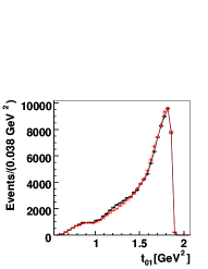
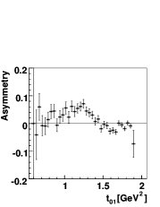
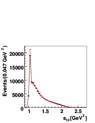
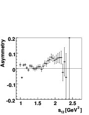
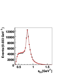
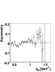
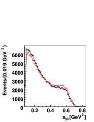
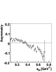
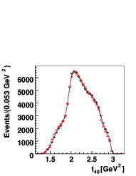
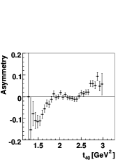
Figure 2: Distributions (left) of 200k simulated events for the 5 kinematical variables shown for $\rm B^{+}$ (solid) and $\rm B^{-}$ (dashed) decays separately. Also shown (right) are the asymmetries between the $\rm B^{+}$ and $\rm B^{-}$ distributions, where the asymmetry is defined as the number of $\rm B^{-}$ decays minus the number of $\rm B^{+}$ decays normalised by the sum.

A log-likelihood function is defined as:

$$\log(\mathcal{L})=\sum\limits_{\mathrm{all\;B^{-}}}\log(P^{-}_{i})+\sum\limits_{\mathrm{all\;B^{+}}}\log(P^{+}_{j}),$$ (17)

where the probability density functions are defined as in expression 16, and the sums run over all B candidates in the sample. The function was maximised for each sample using the MINUIT package [19], with $r_{B}$, $\delta_{B}$ and $\gamma$ as the free parameters. (It is assumed that all parameters associated with the D decay model are known.) Each sample contained 1000 events. A scan of the negative log-likelihood, plotted for $\gamma$ against $\delta_{B}$ is shown for a typical sample in Figure 3. The function is well behaved with a minimum close to the input value and a second solution at $\gamma-180^{\circ}$ and $\delta_{B}-180^{\circ}$. Also shown is a scan for $\gamma$ against $r_{B}$.

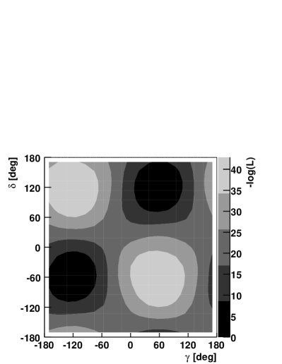
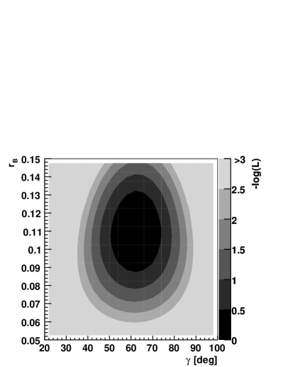
Figure 3: Negative log-likelihood shown for $\gamma$ against $\delta_{B}$ (top) and $\gamma$ against $r_{B}$ (bottom) for a typical simulated experiment of 1000 events. The input values are at $\gamma=60^{\circ}$, $\delta_{B}=130^{\circ}$ and $r_{B}=0.10$.

For each sample the fitted parameters and the assigned errors were recorded. The reliability of the fit result was studied for each variable by constructing the ‘pull distribution’, which is the difference between the fitted and input parameter, divided by the assigned error. The means and RMS widths of the pull distributions are displayed in Table 1 and are seen to be compatible with 0 and 1 respectively. This indicates that the log-likelihood fit is unbiased and the returned errors are reliable. The fit errors are also included in Table 1, averaged over all fits. $\gamma$ is extracted with a precision of $14^{\circ}$. There is very little correlation between the three fit parameters, as is clear from the contours in Figure 3.

Table 1: Result from 218 simulated experiments, showing the average assigned error, and the mean and width of the pull distribution.

	Error		Pull mean		Pull width
$\gamma$	$14.4$$\pm$	$0.7^{\circ}$	$0.13$$\pm$	$0.07$	$1.10$$\pm$	$0.05$
$\delta_{B}$	$14.3$$\pm$	$0.5^{\circ}$	$0.10$$\pm$	$0.07$	$1.09$$\pm$	$0.05$
$r_{B}$	$0.023$$\pm$	$0.001$	$0.11$$\pm$	$0.06$	$0.95$$\pm$	$0.05$

Table 2: Dependence of $\gamma$ fit results on the value of $r_{B}$, showing the average assigned error and the means and widths of the pull distributions.

$r_{B}$	Error		Pull mean		Pull width
$0.05$	$24.4$$\pm$	$0.6^{\circ}$	$0.12$$\pm$	$0.21$	$1.05$$\pm$	$0.15$
$0.10$	$14.4$$\pm$	$0.7^{\circ}$	$0.13$$\pm$	$0.07$	$1.10$$\pm$	$0.05$
$0.15$	$8.8$$\pm$	$0.2^{\circ}$	$0.00$$\pm$	$0.29$	$0.96$$\pm$	$0.21$
$0.20$	$7.2$$\pm$	$0.1^{\circ}$	$-0.06$$\pm$	$0.22$	$1.11$$\pm$	$0.16$

The size of the interference effects in $\rm B^{\pm}\to DK^{\pm}$ decays, and hence the sensitivity of the fit to $\gamma$, depends on the value of $r_{B}$. To investigate this dependence several 1000 event samples were generated with different values of $r_{B}$ between 0.05 and 0.20. These samples were then fitted as previously. The fit result on $\gamma$ and associated uncertainty for each $r_{B}$ value are shown in Table 2. It can be seen that the $\gamma$ error varies approximately linearly with the inverse of $r_{B}$.

Table 3: Statistical uncertainty on $\gamma$ for various values of $R$ and $\Delta\phi$. These parameters are defined in expressions 10 and 11 with the same values being used for $\rm K_{1}(1270)K$, $\rm K_{1}(1270)K$ and $\rm K^{\star}(892)^{0}K\pi$.

$R$	$\Delta\phi$
	$0^{\circ}$	$90^{\circ}$	$180^{\circ}$	$270^{\circ}$
$0$	$14^{\circ}$	/	/	/
$0.25$	$18^{\circ}$	$14^{\circ}$	$19^{\circ}$	$13^{\circ}$
$0.50$	$27^{\circ}$	$13^{\circ}$	$18^{\circ}$	$13^{\circ}$
$1.00$	$23^{\circ}$	$13^{\circ}$	/	$13^{\circ}$
$2.00$	$21^{\circ}$	$14^{\circ}$	$19^{\circ}$	$14^{\circ}$

Table 4: Statistical uncertainty on $\gamma$ for various $R$ values and different $\Delta\phi$ scenarios. The same $R$ values are being used for $\rm K_{1}(1270)K$, $\rm K_{1}(1400)K$ and $\rm K^{\star}(892)^{0}K\pi$. The scenarios for $\Delta\phi$ are given in the text.

$R$	$\Delta\phi$ scenario
	1	2	3	4
$0.25$	$14^{\circ}$	$19^{\circ}$	$14^{\circ}$	$13^{\circ}$
$0.50$	$14^{\circ}$	$17^{\circ}$	$14^{\circ}$	$15^{\circ}$
$1.00$	$12^{\circ}$	$18^{\circ}$	$26^{\circ}$	$20^{\circ}$
$2.00$	$13^{\circ}$	$14^{\circ}$	$16^{\circ}$	$19^{\circ}$

As explained in Section 3.1 the fitted model reported in [12] does not distinguish between the relative contribution of certain $\rm D$ decay amplitudes and their CP-conjugate final states. The importance of this unknown information on the fit sensitivity was assessed by generating and fitting 1000 event simulated datasets with different values of the $R$ and $\Delta\phi$ parameters defined in expressions 10 and 11. In varying these parameters the overall contribution of each mode and its CP-conjugate state, eg. $|A({\rm D^{0}\to K_{1}(1270)^{+}K^{-}})\,+\,A({\rm D^{0}\to K_{1}(1270)^{-}K^{+}})|^{2}$, was kept constant. The results for the uncertainty on $\gamma$ are shown in Table 3 in the case where a common value of $R$ and $\Delta\phi$ is taken for the three final states under consideration. In a further study the phase shift $\Delta\phi$ was allowed to take different values between the three modes. Four scenarios were considered with the following arbitrary (randomly chosen) sets of values for $\Delta\phi_{K_{1}(1270)K}$, $\Delta\phi_{K_{1}(1400)K}$ and $\Delta\phi_{K^{\star}(892)^{0}K\pi}$ respectively:

1. 39^∘, 211^∘ and 115^∘ (default);

2. 53^∘, 108^∘ and 15^∘;

3. 55^∘, 344^∘ and 173^∘;

4. 209^∘, 339^∘ and 87^∘.

The statistical uncertainties found on $\gamma$ for these scenarios are given in Table 4. For both Table 3 and Table 4 only a single experiment was performed at each point in parameter space, hence the stated error carries an uncertainty of a few degrees. However any minor variation in result arising from the exact value of the fitted $r_{B}$ parameter, experiment-to-experiment, has been corrected for by using the dependence observed in the study reported in Table 2.

It can be seen that the precision of the fit is fairly uniform over parameter space, with a typical value of $15^{\circ}$. In certain cases however the precision is worse, particularly when $R=1$ and/or $\Delta\phi=0$. More detailed studies of $\rm D\to K^{+}K^{-}\pi^{+}\pi^{-}$ decays are therefore needed to reliably estimate the instrinsic sensitivity of $\rm B^{\pm}\to(K^{+}K^{-}\pi^{+}\pi^{-})_{D}\,K^{\pm}$ for a $\gamma$ measurement. However, variations in other aspects of the $\rm D\to K^{+}K^{-}\pi^{+}\pi^{-}$ decay structure were found to have limited consequences for the fit precision.

Finally it was investigated what biases would be introduced in the $\gamma$ extraction through incorrect knowledge of the decay model. Experiments were performed in which the datasets were generated with the full model in the default scenario, but fitted with a model which omitted all the decay amplitudes with a contribution less than 3% to the overall rate. Shifts of up to $8^{\circ}$ were observed in the measured value of $\gamma$. This value can be considered as an upper bound to any final systematic uncertainty, as it will be possible to accumulate very large samples of $\rm D\to K^{+}K^{-}\pi^{+}\pi^{-}$ events at the LHC, which will allow the decay model to be refined and improved with respect to the one assumed here. Additional information will also become available from CP-tagged $\rm D$ decays at facilities operating at the $\psi(3770)$ resonance [20].

4 Conclusions

We have shown that the decay $\rm B^{\pm}\to(K^{+}K^{-}\pi^{+}\pi^{-})_{D}\,K^{\pm}$ can be used to provide an interesting measurement of the unitarity triangle angle $\gamma$. With 1000 events and assuming a value of $r_{B}=0.10$ it is possible to measure $\gamma$ with a precision of around $15^{\circ}$. The exact sensitivity achievable depends on the relative contributions of certain unmeasured modes in the $\rm D$ decay model. The final state, involving only charged particles, and kaons in particular, is well suited to LHCb. A full reconstruction study is necessary to estimate reliably the expected event yields and the level of background.

Finally we remark that the same technique of a four-body amplitude analysis in $\rm B^{\pm}\to DK^{\pm}$ decays can be applied to other modes, most notably the ‘ADS’ channel $\rm D\to K^{\pm}\pi^{\mp}\pi^{+}\pi^{-}$.

Acknowlegements

We are grateful to David Asner, Robert Fleischer and Alberto Reis for valuable discussions. We also acknowledge the support of the Particle Physics and Astronomy Research Council, UK.

References

• [1] L. Wolfenstein, Phys. Rev. Lett. 51, (1993) 1945.
• [2] M. Gronau and D. London, Phys. Lett. B 253, (1991) 483; M. Gronau and D. Wyler, Phys. Lett. B 265, (1991) 172.
• [3] D. Atwood, I. Dunietz and A. Soni, Phys. Rev. Lett. 78 (1997) 3257; D. Atwood, I. Dunietz and A. Soni, Phys. Rev. D 63 (2001) 036005.
• [4] A. Giri, Y. Grossman, A. Soffer and J. Zupan, Phys. Rev. D 68 (2003) 054018.
• [5] Y. Grossman, Z. Ligeti and A. Soffer, Phys. Rev. D 67 (2003) 071301.
• [6] BABAR Collaboration, B. Aubert et al., hep-ex/0607104; Phys. Rev. Lett 95 (2005) 121802.
• [7] Belle Collaboration, A. Poluektov et al., Phys. Rev. D 73 (2006) 112009; Phys. Rev. D 70 (2004) 072003.
• [8] CKMfitter Group, J. Charles et al., Eur. Phys. J. C 41 (2004) 1. Updated results at http://www.slac.standford.edu/xorg/
• [9] UTFit Collaboration, M. Bona et al., JHEP 0507 (2005) 028. Updated results at http://www.utfit.org
• [10] BABAR Collaboration, B. Aubert et al., Phys. Rev. D 72 (2005) 032004; Phys. Rev. D 73 (2006) 051105.
• [11] BELLE Collaboration, K. Abe et al., hep-ex/0508048; Phys. Rev. D 73 (2006) 051106.
• [12] FOCUS Collaboration, J. Link et al., Phys. Lett. B 610 (2005) 225.
• [13] E791 Collaboration, E.M. Aitala et al., Phys. Lett. B 423 (1998) 185.
• [14] W.M. Yao et al., Journal of Physics G 33, (2006) 1.
• [15] LHCb Collaboration, LHCC-2003-030, CERN, Geneva.
• [16] J.M. Blatt and V.F. Weisskopf, Theoretical Nuclear Physics, John Wiley & Sons, New York, 1952.
• [17] E. Byckling and K. Kajantie, Particle Kinematics, John Wiley & Sons, New York, 1973.
• [18] MARK-III Collaboration, D.Β Coffman et al., Phys.Β Rev.Β D 45 (1992) 2196.
• [19] F. James, MINUIT: function minimization and error analysis, CERN, Geneva 1994.
• [20] See for example a discussion of the use of CP-tagged $\rm D^{0}$ decays in a $\rm D\to K_{S}\pi^{+}\pi^{-}$ analysis: A. Bondar and A. Poluektov, Eur. Phys. J. C47 (2006) 347.