Abstract

In this article, we take the point of view that the charmed axial-vector meson $D_{s1}(2460)$ is the conventional $c\bar{s}$ meson and calculate the strong coupling constant $g_{D_{s1}D^{*}K}$ in the framework of the light-cone QCD sum rules approach. The numerical values of strong coupling constants $g_{D_{s1}D^{*}K}$ and $g_{D_{s0}DK}$ are very large, and support the hadronic dressing mechanism. Just like the scalar mesons $f_{0}(980)$ and $a_{0}(980)$, the scalar meson $D_{s0}(2317)$ and axial-vector meson $D_{s1}(2460)$ may have small $c\bar{s}$ kernels of the typical $c\bar{s}$ meson size, the strong couplings to the hadronic channels (or the virtual mesons loops) may result in smaller masses than the conventional $c\bar{s}$ mesons in the constituent quark models, and enrich the pure $c\bar{s}$ states with other components.

PACS numbers: 12.38.Lg; 13.25.Jx; 14.40.Cs

Key Words: $D_{s1}(2460)$, light-cone QCD sum rules

1 Introduction

The two strange-charmed mesons $D_{s0}(2317)$ and $D_{s1}(2460)$ with the spin-parity $0^{+}$ and $1^{+}$ respectively can not be comfortably identified as the quark-antiquark bound states in the spectrum of the constituent quark models, they have triggered hot debate on their nature, under-structures and whether it is necessary to introduce the exotic states [1, 2]. The masses of the $D_{s0}(2317)$ and $D_{s1}(2460)$ are significantly lower than the masses of the $0^{+}$ and $1^{+}$ states respectively from the quark models and lattice simulations [3]. The difficulties to identify the $D_{s0}(2317)$ and $D_{s1}(2460)$ states with the conventional $c\overline{s}$ mesons are rather similar to those appearing in the light scalar mesons below $1GeV$. The light scalar mesons are the subject of an intense and continuous controversy in clarifying the hadron spectroscopy[4], the more elusive things are the constituent structures of the $f_{0}(980)$ and $a_{0}(980)$ mesons with almost the degenerate masses. The mesons $D_{s0}(2317)$ and $D_{s1}(2460)$ lie just below the $DK$ and $D^{\ast}K$ threshold respectively, which are analogous to the situation that the scalar mesons $a_{0}(980)$ and $f_{0}(980)$ lie just below the $K\bar{K}$ threshold and couple strongly to the nearby channels. The mechanism responsible for the low-mass charmed mesons may be the same as the light scalar nonet mesons, the $f_{0}(600)$, $f_{0}(980)$, $a_{0}(980)$ and $K^{\ast}_{0}(800)$ [5, 6, 7, 8]. There have been a lot of explanations for their nature, for example, the conventional $c\bar{s}$ states [9, 10], two-meson molecular states [11], four-quark states [12], etc. If we take the scalar mesons $a_{0}(980)$ and $f_{0}(980)$ as four quark states with the constituents of scalar diquark-antidiquark sub-structures, the masses of the scalar nonet mesons below $1GeV$ can be naturally explained [7, 8].

There are other possibilities besides the four-quark state explanations, for example, the scalar mesons $a_{0}(980)$, $f_{0}(980)$, $D_{s0}(2317)$ and the axial-vector meson $D_{s1}(2460)$ may have bare $P-$wave $q\overline{q}$ and $c\bar{s}$ kernels with strong coupling to the nearby thresholds respectively, the $S-$wave virtual intermediate hadronic states (or the virtual mesons loops) play a crucial role in the composition of those bound states (or resonances due to the masses below or above the thresholds). The hadronic dressing mechanism (or unitarized quark models) takes the point of view that the mesons $f_{0}(980)$, $a_{0}(980)$, $D_{s0}(2317)$ and $D_{s1}(2460)$ have small $q\bar{q}$ and $c\bar{s}$ kernels of the typical $q\bar{q}$ and $c\bar{s}$ mesons size respectively. The strong couplings to the virtual intermediate hadronic states (or the virtual mesons loops) may result in smaller masses than the conventional scalar $q\bar{q}$ and $c\bar{s}$ mesons in the constituent quark models, enrich the pure $q\bar{q}$ and $c\bar{s}$ states with other components [13, 14]. Those mesons may spend part (or most part) of their lifetime as virtual $K\bar{K}$, $DK$ and $D^{*}K$ states [5, 6, 13, 14]. Despite what constituents they may have, we have the fact that they lie just a little below the $K\bar{K}$, $DK$ and $D^{*}K$ thresholds respectively, the strong interactions with the $K\bar{K}$, $DK$ and $D^{*}K$ thresholds will significantly influence their dynamics, although the decays $D_{s0}(2317)\rightarrow DK$ and $D_{s1}(2460)\rightarrow D^{*}K$ are kinematically suppressed. It is interesting to investigate the possibility of the hadronic dressing mechanism.

In our previous work, we take the point of view that the scalar mesons $f_{0}(980)$, $a_{0}(980)$ and $D_{s0}(2317)$ are the conventional $q\bar{q}$ and $c\bar{s}$ state respectively, and calculate the values of the strong coupling constants $g_{f_{0}KK}$, $g_{a_{0}KK}$, and $g_{D_{s0}DK}$ within the framework of the light-cone QCD sum rules approach [5, 6]. The large values of the strong coupling constants support the hadronic dressing mechanism. In this article, we take the axial-vector meson $D_{s1}(2460)$ as the conventional $c\bar{s}$ state, and calculate the value of the strong coupling constant $g_{D_{s1}D^{*}K}$ in the framework of the light-cone QCD sum rules approach and study the possibility of the hadronic dressing mechanism in the axial-vector channel. The light-cone QCD sum rules approach carries out the operator product expansion near the light-cone $x^{2}\approx 0$ instead of the short distance $x\approx 0$ while the non-perturbative matrix elements are parameterized by the light-cone distribution amplitudes which classified according to their twists instead of the vacuum condensates [15, 16]. The non-perturbative parameters in the light-cone distribution amplitudes are calculated by the conventional QCD sum rules and the values are universal [17].

The article is arranged as: in Section 2, we derive the strong coupling constant $g_{D_{s1}D^{*}K}$ within the framework of the light-cone QCD sum rules approach; in Section 3, the numerical result and discussion; and in Section 4, conclusion.

2 Strong coupling constant $g_{D_{s1}D^{*}K}$ with light-cone QCD sum rules

In the following, we write down the definition for the strong coupling constant $g_{D_{s1}D^{*}K}$ ,

$$\langle D_{s1}(p+q)|D^{*}(p)K(q)\rangle=-ig_{D_{s1}D^{*}K}\eta^{*}_{\alpha}\epsilon^{\alpha}=-iM_{D_{s1}}\hat{g}_{D_{s1}D^{*}K}\eta^{*}_{\alpha}\epsilon^{\alpha}\,\,,$$ (1)

where the $\epsilon_{\alpha}$ and $\eta_{\alpha}$ are the polarization vectors of the mesons $D^{*}$ and $D_{s1}(2460)$ respectively. The mass of the $D_{s1}(2460)$ $M_{D_{s1}}$ can serve as an energy scale, we factorize the $M_{D_{s1}}$ from the $g_{D_{s1}D^{*}K}$. We study the strong coupling constant $g_{D_{s1}D^{*}K}$ with the two-point correlation function $\Pi_{\mu\nu}(p,q)$,

$$\Pi_{\mu\nu}(p,q) = i\int d^{4}x\,e^{-iq\cdot x}\,\langle 0|T\left\{J^{V}_{\mu}(0){J^{A}_{\nu}}^{+}(x)\right\}|K(p)\rangle\,,$$ (2)

$$J^{V}_{\mu}(x) = {\bar{u}}(x)\gamma_{\mu}c(x)\,,$$ (3)

$$J^{A}_{\mu}(x) = {\bar{s}}(x)\gamma_{\mu}\gamma_{5}c(x)\,,$$ (4)

where the vector current $J^{V}_{\mu}(x)$ and the axial-vector current $J^{A}_{\mu}(x)$ interpolate the vector meson $D^{*}$ and the axial-vector meson $D_{s1}(2460)$ respectively, the external $K$ state has four momentum $p_{\mu}$ with $p^{2}=m_{K}^{2}$. The correlation function $\Pi_{\mu\nu}(p,q)$ can be decomposed as

$$\Pi_{\mu\nu}(p,q) = i\Pi g_{\mu\nu}+\Pi_{1}(p_{\mu}q_{\nu}+p_{\nu}q_{\mu})+\cdots$$ (5)

due to the Lorentz invariance.

According to the basic assumption of current-hadron duality in the QCD sum rules approach [17], we can insert a complete series of intermediate states with the same quantum numbers as the current operators $J^{V}_{\mu}(x)$ and $J^{A}_{\mu}(x)$ into the correlation function $\Pi_{\mu\nu}(p,q)$ to obtain the hadronic representation. After isolating the ground state contributions from the pole terms of the mesons $D_{s1}(2460)$ and $D^{*}$, we get the following result,

$$\Pi_{\mu\nu} = \frac{\langle 0|J^{V}_{\mu}(0)\mid D^{*}(q+p)\rangle\langle D^{*}|D_{s1}K\rangle\langle D_{s1}(q)|{J^{A}_{\nu}}^{+}(0)|0\rangle}{\left[M_{D^{*}}^{2}-(q+p)^{2}\right]\left[M_{D_{s1}}^{2}-q^{2}\right]}+\cdots$$ (6)

$$= -\frac{ig_{D_{s1}D^{*}K}f_{D^{*}}f_{D_{s1}}M_{D^{*}}M_{D_{s1}}}{\left[M_{D^{*}}^{2}-(q+p)^{2}\right]\left[M_{D_{s1}}^{2}-q^{2}\right]}g_{\mu\nu}+\cdots,$$

where the following definitions have been used,

$$\langle 0|J^{V}_{\mu}(0)|D^{*}\rangle = f_{D^{*}}M_{D^{*}}\epsilon_{\mu}\,,$$

$$\langle 0|J^{A}_{\mu}(0)|D_{s1}\rangle = f_{D_{s1}}M_{D_{s1}}\eta_{\mu}\,,$$

here the $f_{D^{*}}$ and $f_{D_{s1}}$ are the weak decay constants of the $D^{*}$ and $D_{s1}(2460)$ respectively. The vector current $J^{V}_{\mu}(x)$ and axial-vector current $J^{A}_{\mu}(x)$ have non-vanishing couplings to the scalar meson $D_{0}$ and pseudoscalar meson $D_{s}$, respectively,

$$\langle 0|J^{V}_{\mu}(0)|D_{0}(q)\rangle = f_{D_{0}}q_{\mu}\,,$$

$$\langle 0|J^{A}_{\mu}(0)|D_{s}(q)\rangle = if_{D_{s}}q_{\mu}\,,$$

where the $f_{D_{0}}$ and $f_{D_{s}}$ are the weak decay constants. The $\Pi_{1}$ with the tensor structure $p_{\mu}q_{\nu}+p_{\nu}q_{\mu}$ receives contribution from the mesons $D_{0}$ and $D_{s}$ besides the $D^{*}$ and $D_{s1}(2460)$, we choose the tensor structure $g_{\mu\nu}$ for analysis to avoid possible contaminations from the scalar and pseudoscalar mesons. In Eq.(6), we have not shown the contributions from the high resonances and continuum states explicitly as they are suppressed due to the double Borel transformation.

In the following, we briefly outline the operator product expansion for the correlation function $\Pi_{\mu\nu}(p,q)$ in perturbative QCD theory. The calculations are performed at the large space-like momentum regions $(q+p)^{2}\ll 0$ and $q^{2}\ll 0$, which correspond to the small light-cone distance $x^{2}\approx 0$ required by the validity of the operator product expansion approach. We write down the propagator of a massive quark in the external gluon field in the Fock-Schwinger gauge firstly [18],

$$\langle 0|T\{q_{i}(x_{1})\,\bar{q}_{j}(x_{2})\}|0\rangle = i\int\frac{d^{4}k}{(2\pi)^{4}}e^{-ik(x_{1}-x_{2})}$$ (7)

$$\left\{\frac{\not\!k+m}{k^{2}-m^{2}}\delta_{ij}-\int\limits_{0}^{1}dv\,g_{s}\,G^{\mu\nu}_{ij}(vx_{1}+(1-v)x_{2})\right.$$

$$\left.\Big{[}\frac{1}{2}\frac{\not\!k+m}{(k^{2}-m^{2})^{2}}\sigma_{\mu\nu}-\frac{1}{k^{2}-m^{2}}v(x_{1}-x_{2})_{\mu}\gamma_{\nu}\Big{]}\right\}\,,$$

where the $G_{\mu\nu}$ is the gluonic field strength, and the $g_{s}$ denotes the strong coupling constant. Substituting the above $c$ quark propagator and the corresponding $K$ meson light-cone distribution amplitudes into the correlation function $\Pi_{\mu\nu}(p,q)$ in Eq.(2) and completing the integrals over the variables $x$ and $k$, finally we obtain the analytical result, which is given explicitly in the appendix.

In calculation, the two-particle and three-particle $K$ meson light-cone distribution amplitudes have been used [15, 16, 18, 19, 20], the explicitly expressions are given in the appendix. The parameters in the light-cone distribution amplitudes are scale dependent and can be estimated with the QCD sum rules approach [15, 16, 18, 19, 20]. In this article, the energy scale $\mu$ is chosen to be $\mu=1GeV$.

Now we perform the double Borel transformation with respect to the variables $Q_{1}^{2}=-q^{2}$ and $Q_{2}^{2}=-(p+q)^{2}$ for the correlation function $\Pi$ in Eq.(6), and obtain the analytical expression of the invariant function in the hadronic representation,

$$B_{M_{2}^{2}}B_{M_{1}^{2}}\Pi = -i\frac{g_{D_{s1}D^{*}K}f_{D^{*}}f_{D_{s1}}M_{D^{*}}M_{D_{s1}}}{M_{1}^{2}M_{2}^{2}}\exp\left[-\frac{M^{2}_{D_{s1}}}{M_{1}^{2}}-\frac{M^{2}_{D^{*}}}{M_{2}^{2}}\right]+\cdots,$$ (8)

here we have not shown the contributions from the high resonances and continuum states explicitly for simplicity. In order to match the duality regions below the thresholds $s_{0}$ and $s_{0}^{\prime}$ for the interpolating currents $J^{V}_{\mu}(x)$ and $J^{A}_{\mu}(x)$ respectively, we can express the correlation function $\Pi$ at the level of quark-gluon degrees of freedom into the following form,

$$\Pi = \int dsds^{\prime}\frac{\rho(s,s^{\prime})}{[s-(q+p)^{2}][s^{\prime}-q^{2}]}\,,$$ (9)

then perform the double Borel transformation with respect to the variables $Q_{1}^{2}$ and $Q_{2}^{2}$ directly. However, the analytical expression of the spectral density $\rho(s,s^{\prime})$ is hard to obtain, we have to resort to some approximations. As the contributions from the higher twist terms are suppressed by more powers of $\frac{1}{m_{c}^{2}-(q+up)^{2}}$, the net contributions of the three-particle (quark-antiquark-gluon) twist-3 and twist-4 terms are of minor importance, about $20\%$, the continuum subtractions will not affect the results remarkably. The dominating contribution comes from the two-particle twist-3 term involving the $\varphi_{p}(u)$. We preform the same trick as Refs.[18, 21] and expand the amplitude $\varphi_{p}(u)$ in terms of polynomials of $1-u$,

$$\varphi_{p}(u)=\sum_{k=0}^{N}b_{k}(1-u)^{k}=\sum_{k=0}^{N}b_{k}\left(\frac{s-m_{c}^{2}}{s-q^{2}}\right)^{k},$$ (10)

then introduce the variable $s^{\prime}$ and the spectral density is obtained. In the decay $B\to\chi_{c0}K$, the factorizable contribution is zero and the non-factorizable contributions from the soft hadronic matrix elements are too small to accommodate the experimental data [22], the contributions of the three-particle (quark-antiquark-gluon) distribution amplitudes of the mesons are always of minor importance comparing with the two-particle (quark-antiquark) distribution amplitudes in the light-cone QCD sum rules. In our previous work, we study the four form-factors $f_{1}(Q^{2})$, $f_{2}(Q^{2})$, $g_{1}(Q^{2})$ and $g_{2}(Q^{2})$ of the $\Sigma\to n$ in the framework of the light-cone QCD sum rules approach up to twist-6 three-quark light-cone distribution amplitudes and obtain satisfactory results [23]. In the light-cone QCD sum rules, we can neglect the contributions from the valence gluons and make relatively rough estimations.

After straightforward calculations, we obtain the final expression of the double Borel transformed correlation function $\Pi(M_{1}^{2},M_{2}^{2})$ at the level of quark-gluon degrees of freedom. The masses of the charmed mesons are $M_{D_{s1}}=2.46GeV$ and $M_{D^{*}}=2.01GeV$, $\frac{M_{D^{*}}}{M_{D^{*}}+M_{D_{s1}}}\approx 0.45$, there exists an overlapping working window for the two Borel parameters $M_{1}^{2}$ and $M_{2}^{2}$, it’s convenient to take the value $M_{1}^{2}=M_{2}^{2}$. We introduce the threshold parameter $s_{0}$ and make the simple replacement,

$$e^{-\frac{m_{c}^{2}+u_{0}(1-u_{0})m_{K}^{2}}{M^{2}}}\rightarrow e^{-\frac{m_{c}^{2}+u_{0}(1-u_{0})m_{K}^{2}}{M^{2}}}-e^{-\frac{s_{0}}{M^{2}}}$$

to subtract the contributions from the high resonances and continuum states [18], finally we obtain the sum rule for the strong coupling constant $g_{D_{s1}D^{*}K}$,

$$g_{D_{s1}D^{*}K} = \frac{1}{f_{D^{*}}f_{D_{s1}}M_{D^{*}}M_{D_{s1}}}\exp\left(\frac{M^{2}_{D_{s1}}}{M_{1}^{2}}+\frac{M^{2}_{D^{*}}}{M_{2}^{2}}\right)\left\{\left[\exp\left(-\frac{BB}{M^{2}}\right)-\exp\left(-\frac{s_{0}}{M^{2}}\right)\right]\right.$$ (11)

$$f_{K}\left[\frac{m_{c}m_{K}^{2}M^{2}}{m_{u}+m_{s}}\varphi_{p}(u_{0})+\frac{m_{K}^{2}(M^{2}+m_{c}^{2})}{8}\frac{d}{du_{0}}A(u_{0})-\frac{M^{4}}{2}\frac{d}{du_{0}}\phi_{K}(u_{0})\right]$$

$$-\exp\left(-\frac{BB}{M^{2}}\right)\left[f_{K}m_{c}^{2}m_{K}^{2}\int_{0}^{u_{0}}dtB(t)\right.$$

$$+m_{K}^{2}\int_{0}^{u_{0}}d\alpha_{s}\int_{u_{0}-\alpha_{s}}^{1-\alpha_{s}}d\alpha_{g}\frac{(u_{0}f_{K}m_{K}^{2}\Phi+f_{3K}m_{c}\phi_{3K})(1-\alpha_{s}-\alpha_{g},\alpha_{s},\alpha_{g})}{\alpha_{g}}$$

$$+f_{K}m_{K}^{2}M^{2}\frac{d}{du_{0}}\int_{0}^{u_{0}}d\alpha_{s}\int_{u_{0}-\alpha_{s}}^{1-\alpha_{s}}d\alpha_{g}\frac{(A_{\parallel}-V_{\parallel})(1-\alpha_{s}-\alpha_{g},\alpha_{s},\alpha_{g})}{2\alpha_{g}}$$

$$-f_{K}m_{K}^{2}M^{2}\frac{d}{du_{0}}\int_{0}^{u_{0}}d\alpha_{s}\int_{u_{0}-\alpha_{s}}^{1-\alpha_{s}}d\alpha_{g}A_{\parallel}(1-\alpha_{s}-\alpha_{g},\alpha_{s},\alpha_{g})\frac{\alpha_{s}+\alpha_{g}-u_{0}}{\alpha_{g}^{2}}$$

$$+f_{K}m_{K}^{4}\left(\int_{0}^{1-u_{0}}d\alpha_{g}\int^{u_{0}}_{u_{0}-\alpha_{g}}d\alpha_{s}\int_{0}^{\alpha_{s}}d\alpha+\int^{1}_{1-u_{0}}d\alpha_{g}\int^{1-\alpha_{g}}_{u_{0}-\alpha_{g}}d\alpha_{s}\int_{0}^{\alpha_{s}}d\alpha\right)$$

$$\left[\frac{1}{\alpha_{g}}\left(3-\frac{2m_{c}^{2}}{M^{2}}\right)\Phi+\frac{4m_{c}^{2}}{M^{2}}\frac{\alpha_{s}+\alpha_{g}-u_{0}}{\alpha_{g}^{2}}(A_{\perp}+A_{\parallel})\right](1-\alpha-\alpha_{g},\alpha,\alpha_{g})$$

$$-f_{K}m_{K}^{4}u_{0}\frac{d}{du_{0}}\left(\int_{0}^{1-u_{0}}d\alpha_{g}\int^{u_{0}}_{u_{0}-\alpha_{g}}d\alpha_{s}\int_{0}^{\alpha_{s}}d\alpha+\int^{1}_{1-u_{0}}d\alpha_{g}\int^{1-\alpha_{g}}_{u_{0}-\alpha_{g}}d\alpha_{s}\int_{0}^{\alpha_{s}}d\alpha\right)$$

$$\frac{\Phi(1-\alpha-\alpha_{g},\alpha,\alpha_{g})}{\alpha_{g}}$$

$$-f_{K}m_{K}^{4}\int_{1-u_{0}}^{1}d\alpha_{g}\int_{0}^{\alpha_{g}}d\beta\int_{0}^{1-\beta}d\alpha\left[\Phi(1-\alpha-\beta,\alpha,\beta)\frac{1-u_{0}}{\alpha_{g}^{2}}\left(4-\frac{2m_{c}^{2}}{M^{2}}\right)\right.$$

$$\left.+\frac{4m_{c}^{2}}{M^{2}}\frac{(1-u_{0})^{2}}{\alpha_{g}^{3}}(A_{\parallel}+A_{\perp})(1-\alpha-\beta,\alpha,\beta)\right]$$

$$\left.\left.+f_{K}m_{K}^{4}\frac{d}{du_{0}}\int_{1-u_{0}}^{1}d\alpha_{g}\int_{0}^{\alpha_{g}}d\beta\int_{0}^{1-\beta}d\alpha\Phi(1-\alpha-\beta,\alpha,\beta)\frac{u_{0}(1-u_{0})}{\alpha_{g}^{2}}\right]\right\},$$

where

$$BB = m_{c}^{2}+u_{0}(1-u_{0})m_{K}^{2}\,,$$

$$u_{0} = \frac{M_{1}^{2}}{M_{1}^{2}+M_{2}^{2}}\,,$$

$$M^{2} = \frac{M_{1}^{2}M_{2}^{2}}{M_{1}^{2}+M_{2}^{2}}\,,$$ (12)

here we write down only the analytical result without the technical details . The term proportional to the $M^{4}\frac{d}{du_{0}}\phi_{K}(u_{0})$ in Eq.(11) depends heavily on the asymmetry coefficient $a_{1}(\mu)$ of the twist-2 light-cone distribution amplitude $\phi_{K}(u)$ in the limit $u_{0}=\frac{1}{2}$, if we take the value $a_{1}(\mu)=0.06\pm 0.03$ [19, 20], no stable sum rules can be obtained, the value of the $g_{D_{s1}D^{*}K}$ changes significantly with the variation of the Borel parameter $M^{2}$. In this article, we take the assumption that the $u$ and $s$ quarks have symmetric momentum distributions and neglect the coefficient $a_{1}(\mu)$. The existence of such a term is not a bad thing. The $D_{s1}(2460)$ lies below the $D^{*}K$ threshold, it is impossible to measure the strong coupling constant $g_{D_{s1}D^{*}K}$ directly, the corresponding beauty doublet $(0^{+},1^{+})$ $B_{s0}$ and $B_{s1}$ may lie above the $BK$ and $B^{*}K$ thresholds respectively. Once the experimental data of the $B_{s0}$, $B_{s1}$ and the related strong coupling constants are available, we can compare the values of the $g_{B_{s1}B^{*}K}$ from the QCD sum rules with the ones from the experiment, and verify whether or not the coefficient $a_{1}(\mu)$ can be safely neglected. That will put severe constraint on the value of the $a_{1}(\mu)$. With the simple replacement

$$m_{c} \rightarrow m_{b}\,,$$

$$M_{D_{s1}} \rightarrow M_{B_{s1}}\,,$$

$$M_{D^{*}} \rightarrow M_{B^{*}}\,,$$

$$f_{D_{s1}} \rightarrow f_{B_{s1}}\,,$$

$$f_{D^{*}} \rightarrow f_{B^{*}}$$ (13)

in Eq.(11), we can obtain the QCD sum rule for the strong coupling constant $g_{B_{s1}B^{*}K}$.

3 Numerical result and discussion

The parameters are taken as $m_{s}=(140\pm 10)MeV$, $m_{q}=(5.6\pm 1.6)MeV$, $m_{c}=(1.25\pm 0.10)GeV$, $\lambda_{3}=1.6\pm 0.4$, $f_{3K}=(0.45\pm 0.15)\times 10^{-2}GeV^{2}$, $\omega_{3}=-1.2\pm 0.7$, $\eta_{4}=0.6\pm 0.2$, $\omega_{4}=0.2\pm 0.1$, $a_{2}=0.25\pm 0.15$ [15, 16, 18, 19, 20], $f_{K}=0.160GeV$, $m_{K}=498MeV$, $M_{D_{s1}}(2460)=2.46GeV$, $M_{D^{*}}=2.01GeV$, $f_{D^{*}}=(0.24\pm 0.02)GeV$ [18], and $f_{D_{s1}}=(0.225\pm 0.020)GeV$ [10]. The duality threshold $s_{0}$ in Eq.(11) is taken as $s_{0}=(6.8-7.2)GeV^{2}$ to avoid possible contaminations from the high resonances and continuum states, it is reasonable for the narrow $D_{s1}(2460)$ $\sqrt{s_{0}}=(2.6-2.7)GeV>M_{D_{s1}}$, furthermore, in this region, the numerical result is not sensitive to the threshold parameter $s_{0}$. The Borel parameters are chosen as $M_{1}^{2}=M_{2}^{2}=(6-14)GeV^{2}$ and $M^{2}=(3-7)GeV^{2}$, in those regions, the value of the strong coupling constant $g_{D_{s1}D^{*}K}$ is rather stable from the sum rule in Eq.(11) with the simple subtraction, which is shown in Figs.(1-2).

The uncertainties of the four parameters $m_{u}$, $m_{c}$, $\lambda_{3}$ and $\omega_{3}$ can only result in small uncertainties for the numerical values. The main uncertainties come from the seven parameters $f_{3K}$, $m_{s}$, $f_{D^{*}}$, $f_{D_{s1}}$, $a_{2}$, $\eta_{4}$ and $\omega_{4}$, the variations of those parameters (except for the $a_{2}$) can lead to large changes for the numerical values, about $(5-10)\%$, which are shown in the Fig.1. The uncertainties of the three hadronic parameters $f_{3K}$, $f_{D^{*}}$, $f_{D_{s1}}$ and the two light-cone distribution parameters $\eta_{4}$, $\omega_{4}$ can be pined down with the improved QCD sum rules or more experimental data, however, it is a difficult work.

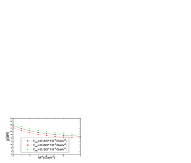
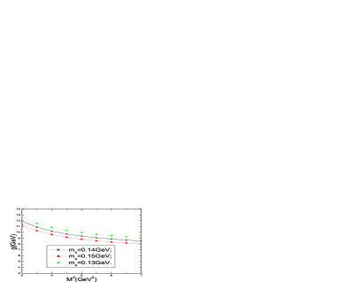
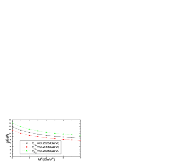
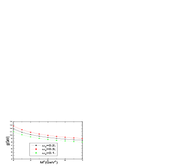
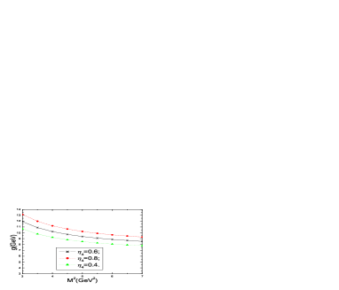
Figure 1: The $g_{D_{s1}D^{*}K}$ with the parameters $f_{3K}$, $m_{s}$, $f_{D^{*}}$, $f_{D_{s1}}$, $\omega_{4}$ and $\eta_{4}$ respectively.

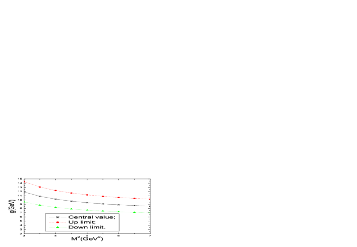
Figure 2: The $g_{D_{s1}D^{*}K}$ with the Borel parameter $M^{2}$.

Taking into account all the uncertainties from the thirteen parameters $m_{s}$, $m_{q}$, $m_{c}$, $\lambda_{3}$, $f_{3K}$, $\omega_{3}$, $\eta_{4}$, $\omega_{4}$, $a_{2}$, $f_{D^{*}}$, $f_{D_{s1}}$, $s_{0}$ and $M^{2}$, finally we obtain the numerical result of the strong coupling constant,

$$g_{D_{s1}D^{*}K} = (10.5\pm 3.5)GeV\,,$$ (14)

$$\hat{g}_{D_{s1}D^{*}K} = 4.3\pm 1.4\,,$$ (15)

the uncertainty is large, about $30\%$. The large values of the strong coupling constants $g_{D_{s0}DK}$ ($g_{D_{s0}DK}=(9.6\pm 2.4)GeV$ [6]) and $g_{D_{s1}D^{*}K}$ obviously support the hadronic dressing mechanism , the scalar meson $D_{s0}(2317)$ and axial-vector meson $D_{s1}(2460)$ (just like the scalar mesons $f_{0}(980)$ and $a_{0}(980)$, see Ref.[5]) can be taken as having small scalar and axial-vector $c\bar{s}$ kernels of typical meson size with large virtual $S$-wave $DK$ and $D^{*}K$ cloud respectively. In Ref.[24], the authors analyze the unitarized two-meson scattering amplitudes from the heavy-light chiral Lagrangian, and observe that the scalar meson $D_{s0}(2317)$ and axial-vector meson $D_{s1}(2460)$ appear as the bound state poles with the strong coupling constants $g_{D_{s0}DK}=10.203GeV$ and $g_{D_{s1}D^{*}K}=10.762GeV$. Our numerical results $g_{D_{s0}DK}=(9.6\pm 2.4)GeV$ and $g_{D_{s1}D^{*}K}=(10.5\pm 3.5)GeV$ are certainly reasonable and can make robust predictions. However, we take the point of view that the meson $D_{s0}(2317)$ ($D_{s1}(2460)$) be bound state in the sense that it appears below the $DK$ ($D^{*}K$) threshold, its constituents may be the bare $c\bar{s}$ state, the virtual $DK$ ($D^{*}K$) pair and their mixing, rather than the $DK$ ($D^{*}K$) bound state. In Ref.[25], the authors take the point of view that the $D_{s0}(2317)$ is the scalar $c\bar{s}$ meson and calculate the mass $M_{D_{s0}}$ with the QCD sum rules approach by taking into account the contribution of the $DK$ continuum, the effects of the $DK$ continuum can pull the mass down remarkably, and the value of the $M_{D_{s0}}$ is in good agreement with experimental data. Our numerical values of the strong coupling constants $g_{D_{s0}DK}$ and $g_{D_{s1}D^{*}K}$ are approximately equal, the spin symmetry of the heavy quarks works rather well, the contribution of the $D^{*}K$ continuum may pull the mass $M_{D_{s1}}$ down remarkably. One can analyze the value of the $M_{D_{s1}}$ in the framework of the QCD sum rules with the axial-vector current $J^{A}_{\mu}(x)$ by including the contribution of the $D^{*}K$ continuum.

4 Conclusion

In this article, we take the point of view that the charmed mesons $D_{s0}(2317)$ and $D_{s1}(2460)$ are the conventional $c\bar{s}$ mesons and calculate the strong coupling constant $g_{D_{s1}D^{*}K}$ within the framework of the light-cone QCD sum rules approach. The numerical values of the strong coupling constants $g_{D_{s1}D^{*}K}$ and $g_{D_{s0}DK}$ are compatible with the existing estimations, the large values support the hadronic dressing mechanism. The uncertainty of the value of the $g_{D_{s1}D^{*}K}$ is large, about $30\%$, it comes from the uncertainties of the thirteen parameters $m_{s}$, $m_{q}$, $m_{c}$, $\lambda_{3}$, $f_{3K}$, $\omega_{3}$, $\eta_{4}$, $\omega_{4}$, $a_{2}$, $f_{D^{*}}$, $f_{D_{s1}}$, $s_{0}$ and $M^{2}$, while the main uncertainty comes from the seven parameters $f_{3K}$, $m_{s}$, $f_{D^{*}}$, $f_{D_{s1}}$, $a_{2}$, $\eta_{4}$ and $\omega_{4}$, the variations of those parameters (except for the $a_{2}$) can lead to large changes for the numerical values, about $(5-10)\%$, refining those parameters is of great importance, improved QCD sum rules and more experimental data may pin down the uncertainties.

Just like the scalar mesons $f_{0}(980)$ and $a_{0}(980)$, the scalar meson $D_{s0}(2317)$ and the axial-vector meson $D_{s1}(2460)$ may have small $c\bar{s}$ kernels of typical $c\bar{s}$ meson size. The strong couplings to virtual intermediate hadronic states (or the virtual mesons loops) can result in smaller masses than the conventional $0^{+}$ and $1^{+}$ mesons in the constituent quark models, enrich the pure $c\bar{s}$ states with other components. The $D_{s0}(2317)$ and $D_{s1}(2460)$ may spend part (or most part) of their lifetimes as virtual $DK$ and $D^{*}K$ states, respectively.

Appendix

The analytical expression of the $\Pi$ at the level of the quark-gluon degrees of freedom,

$$\Pi = -\frac{f_{K}m_{c}m_{K}^{2}}{m_{u}+m_{s}}\int_{0}^{1}du\frac{\varphi_{p}(u)}{AA}+f_{K}m_{c}^{2}m_{K}^{2}\int_{0}^{1}du\int_{0}^{u}dt\frac{B(t)}{AA^{2}}$$ (16)

$$+\frac{f_{K}}{2}\int_{0}^{1}du\left\{\phi_{K}(u)\frac{d}{du}\log AA+\frac{A(u)m_{K}^{2}}{4}\frac{d}{du}\left[\frac{1}{AA}+\frac{m_{c}^{2}}{AA^{2}}\right]\right\}$$

$$+m_{K}^{2}\int_{0}^{1}dv\int_{0}^{1}d\alpha_{g}\int_{0}^{1-\alpha_{g}}d\alpha_{s}$$

$$\frac{\left[f_{K}m_{K}^{2}u\Phi+f_{3K}m_{c}\phi_{3K}\right](1-\alpha_{s}-\alpha_{g},\alpha_{s},\alpha_{g})}{AA^{2}}\mid_{u=\alpha_{s}+(1-v)\alpha_{g}}$$

$$-\frac{f_{K}m_{K}^{2}}{2}\int_{0}^{1}dv\int_{0}^{1}d\alpha_{g}\int_{0}^{1-\alpha_{g}}d\alpha_{s}\left[(1-2v)A_{\parallel}-V_{\parallel}\right](1-\alpha_{s}-\alpha_{g},\alpha_{s},\alpha_{g})$$

$$\frac{d}{du}\frac{1}{AA}\mid_{u=\alpha_{s}+(1-v)\alpha_{g}}$$

$$+f_{K}m_{K}^{4}\int_{0}^{1}dv\int_{0}^{1}d\alpha_{g}\int_{0}^{1-\alpha_{g}}d\alpha_{s}\int_{0}^{\alpha_{s}}d\alpha\Phi(1-\alpha-\alpha_{g},\alpha,\alpha_{g})$$

$$\left\{\frac{4}{AA^{2}}-\frac{4m_{c}^{2}}{AA^{3}}+u\frac{d}{du}\frac{1}{AA^{2}}\right\}_{u=\alpha_{s}+(1-v)\alpha_{g}}$$

$$-f_{K}m_{K}^{4}\int_{0}^{1}dvv\int_{0}^{1}d\alpha_{g}\int_{0}^{\alpha_{g}}d\beta\int_{0}^{1-\beta}d\alpha\Phi(1-\alpha-\beta,\alpha,\beta)$$

$$\left\{\frac{4}{AA^{2}}-\frac{4m_{c}^{2}}{AA^{3}}+u\frac{d}{du}\frac{1}{AA^{2}}\right\}_{u=1-v\alpha_{g}}$$

$$+8f_{K}m_{c}^{2}m_{K}^{4}\int_{0}^{1}dvv\int_{0}^{1}d\alpha_{g}\int_{0}^{1-\alpha_{g}}d\alpha_{s}\int_{0}^{\alpha_{s}}d\alpha(A_{\parallel}+A_{\perp})(1-\alpha-\alpha_{g},\alpha,\alpha_{g})$$

$$\frac{1}{AA^{3}}\mid_{u=\alpha_{s}+(1-v)\alpha_{g}}$$

$$-8f_{K}m_{c}^{2}m_{K}^{4}\int_{0}^{1}dvv^{2}\int_{0}^{1}d\alpha_{g}\int_{0}^{\alpha_{g}}d\beta\int_{0}^{1-\beta}d\alpha(A_{\parallel}+A_{\perp})(1-\alpha-\beta,\alpha,\beta)$$

$$\frac{1}{AA^{3}}\mid_{u=1-v\alpha_{g}}\,\,,$$

where

$$AA = m_{c}^{2}-(q+up)^{2}\,,$$

$$\Phi = A_{\parallel}+A_{\perp}-V_{\parallel}-V_{\perp}\,.$$ (17)

The light-cone distribution amplitudes of the $K$ meson are defined by

$$\langle 0|{\bar{u}}(0)\gamma_{\mu}\gamma_{5}s(x)|K(p)\rangle = if_{K}p_{\mu}\int_{0}^{1}due^{-iup\cdot x}\left\{\phi_{K}(u)+\frac{m_{K}^{2}x^{2}}{16}A(u)\right\}$$

$$+f_{K}m_{K}^{2}\frac{ix_{\mu}}{2p\cdot x}\int_{0}^{1}due^{-iup\cdot x}B(u)\,,$$

$$\langle 0|{\bar{u}}(0)i\gamma_{5}s(x)|K(p)\rangle = \frac{f_{K}m_{K}^{2}}{m_{s}+m_{u}}\int_{0}^{1}due^{-iup\cdot x}\varphi_{p}(u)\,,$$

$$\langle 0|{\bar{u}}(0)\sigma_{\mu\nu}\gamma_{5}s(x)|K(p)\rangle = i(p_{\mu}x_{\nu}-p_{\nu}x_{\mu})\frac{f_{K}m_{K}^{2}}{6(m_{s}+m_{u})}\int_{0}^{1}due^{-iup\cdot x}\varphi_{\sigma}(u)\,,$$

$$\langle 0|{\bar{u}}(0)\sigma_{\alpha\beta}\gamma_{5}g_{s}G_{\mu\nu}(vx)s(x)|K(p)\rangle = f_{3K}\left\{(p_{\mu}p_{\alpha}g^{\bot}_{\nu\beta}-p_{\nu}p_{\alpha}g^{\bot}_{\mu\beta})-(p_{\mu}p_{\beta}g^{\bot}_{\nu\alpha}\right.$$

$$\left.-p_{\nu}p_{\beta}g^{\bot}_{\mu\alpha})\right\}\int{\cal D}\alpha_{i}\phi_{3K}(\alpha_{i})e^{-ip\cdot x(\alpha_{s}+v\alpha_{g})}\,,$$

$$\langle 0|{\bar{u}}(0)\gamma_{\mu}\gamma_{5}g_{s}G_{\alpha\beta}(vx)s(x)|K(p)\rangle = p_{\mu}\frac{p_{\alpha}x_{\beta}-p_{\beta}x_{\alpha}}{p\cdot x}f_{K}m_{K}^{2}$$

$$\int{\cal D}\alpha_{i}A_{\parallel}(\alpha_{i})e^{-ip\cdot x(\alpha_{s}+v\alpha_{g})}$$

$$+f_{K}m_{K}^{2}(p_{\beta}g_{\alpha\mu}-p_{\alpha}g_{\beta\mu})$$

$$\int{\cal D}\alpha_{i}A_{\perp}(\alpha_{i})e^{-ip\cdot x(\alpha_{s}+v\alpha_{g})}\,,$$

$$\langle 0|{\bar{u}}(0)\gamma_{\mu}g_{s}\tilde{G}_{\alpha\beta}(vx)s(x)|K(p)\rangle = p_{\mu}\frac{p_{\alpha}x_{\beta}-p_{\beta}x_{\alpha}}{p\cdot x}f_{K}m_{K}^{2}$$ (18)

$$\int{\cal D}\alpha_{i}V_{\parallel}(\alpha_{i})e^{-ip\cdot x(\alpha_{s}+v\alpha_{g})}$$

$$+f_{K}m_{K}^{2}(p_{\beta}g_{\alpha\mu}-p_{\alpha}g_{\beta\mu})$$

$$\int{\cal D}\alpha_{i}V_{\perp}(\alpha_{i})e^{-ip\cdot x(\alpha_{s}+v\alpha_{g})}\,,$$

where the operator $\tilde{G}_{\alpha\beta}$ is the dual of the $G_{\alpha\beta}$, $\tilde{G}_{\alpha\beta}={1\over 2}\epsilon_{\alpha\beta\mu\nu}G^{\mu\nu}$ and ${\cal{D}}\alpha_{i}$ is defined as ${\cal{D}}\alpha_{i}=d\alpha_{1}d\alpha_{2}d\alpha_{3}\delta(1-\alpha_{1}-\alpha_{2}-\alpha_{3})$. The light-cone distribution amplitudes are parameterized as

$$\phi_{K}(u,\mu) = 6u(1-u)\left\{1+a_{1}C^{\frac{3}{2}}_{1}(2u-1)+a_{2}C^{\frac{3}{2}}_{2}(2u-1)+a_{4}C^{\frac{3}{2}}_{4}(2u-1)\right\}\,,$$

$$\varphi_{p}(u,\mu) = 1+\left\{30\eta_{3}-\frac{5}{2}\rho^{2}\right\}C_{2}^{\frac{1}{2}}(2u-1)$$

$$+\left\{-3\eta_{3}\omega_{3}-\frac{27}{20}\rho^{2}-\frac{81}{10}\rho^{2}a_{2}\right\}C_{4}^{\frac{1}{2}}(2u-1)\,,$$

$$\varphi_{\sigma}(u,\mu) = 6u(1-u)\left\{1+\left[5\eta_{3}-\frac{1}{2}\eta_{3}\omega_{3}-\frac{7}{20}\rho^{2}-\frac{3}{5}\rho^{2}a_{2}\right]C_{2}^{\frac{3}{2}}(2u-1)\right\}\,,$$

$$\phi_{3K}(\alpha_{i},\mu) = 360\alpha_{u}\alpha_{s}\alpha_{g}^{2}\left\{1+\lambda_{3}(\alpha_{u}-\alpha_{s})+\omega_{3}\frac{1}{2}(7\alpha_{g}-3)\right\}\,,$$

$$V_{\parallel}(\alpha_{i},\mu) = 120\alpha_{u}\alpha_{s}\alpha_{g}\left(v_{00}+v_{10}(3\alpha_{g}-1)\right)\,,$$

$$A_{\parallel}(\alpha_{i},\mu) = 120\alpha_{u}\alpha_{s}\alpha_{g}a_{10}(\alpha_{s}-\alpha_{u})\,,$$

$$V_{\perp}(\alpha_{i},\mu) = -30\alpha_{g}^{2}\left\{h_{00}(1-\alpha_{g})+h_{01}\left[\alpha_{g}(1-\alpha_{g})-6\alpha_{u}\alpha_{s}\right]\right.$$

$$\left.+h_{10}\left[\alpha_{g}(1-\alpha_{g})-\frac{3}{2}\left(\alpha_{u}^{2}+\alpha_{s}^{2}\right)\right]\right\}\,,$$

$$A_{\perp}(\alpha_{i},\mu) = 30\alpha_{g}^{2}(\alpha_{u}-\alpha_{s})\left\{h_{00}+h_{01}\alpha_{g}+\frac{1}{2}h_{10}(5\alpha_{g}-3)\right\},$$

$$A(u,\mu) = 6u(1-u)\left\{\frac{16}{15}+\frac{24}{35}a_{2}+20\eta_{3}+\frac{20}{9}\eta_{4}\right.$$

$$+\left[-\frac{1}{15}+\frac{1}{16}-\frac{7}{27}\eta_{3}\omega_{3}-\frac{10}{27}\eta_{4}\right]C^{\frac{3}{2}}_{2}(2u-1)$$

$$\left.+\left[-\frac{11}{210}a_{2}-\frac{4}{135}\eta_{3}\omega_{3}\right]C^{\frac{3}{2}}_{4}(2u-1)\right\}+\left\{-\frac{18}{5}a_{2}+21\eta_{4}\omega_{4}\right\}$$

$$\left\{2u^{3}(10-15u+6u^{2})\log u+2\bar{u}^{3}(10-15\bar{u}+6\bar{u}^{2})\log\bar{u}\right.$$

$$\left.+u\bar{u}(2+13u\bar{u})\right\}\,,$$

$$g_{K}(u,\mu) = 1+g_{2}C^{\frac{1}{2}}_{2}(2u-1)+g_{4}C^{\frac{1}{2}}_{4}(2u-1)\,,$$

$$B(u,\mu) = g_{K}(u,\mu)-\phi_{K}(u,\mu)\,,$$ (19)

where

$$h_{00} = v_{00}=-\frac{\eta_{4}}{3}\,,$$

$$a_{10} = \frac{21}{8}\eta_{4}\omega_{4}-\frac{9}{20}a_{2}\,,$$

$$v_{10} = \frac{21}{8}\eta_{4}\omega_{4}\,,$$

$$h_{01} = \frac{7}{4}\eta_{4}\omega_{4}-\frac{3}{20}a_{2}\,,$$

$$h_{10} = \frac{7}{2}\eta_{4}\omega_{4}+\frac{3}{20}a_{2}\,,$$

$$g_{2} = 1+\frac{18}{7}a_{2}+60\eta_{3}+\frac{20}{3}\eta_{4}\,,$$

$$g_{4} = -\frac{9}{28}a_{2}-6\eta_{3}\omega_{3}\,,$$ (20)

here $C_{2}^{\frac{1}{2}}$, $C_{4}^{\frac{1}{2}}$ and $C_{2}^{\frac{3}{2}}$ are Gegenbauer polynomials, $\eta_{3}=\frac{f_{3K}}{f_{K}}\frac{m_{q}+m_{s}}{M_{K}^{2}}$ and $\rho^{2}={m_{s}^{2}\over M_{K}^{2}}$ [15, 16, 18, 19, 20].

References

- [1] B. Aubert et al [BABAR Collaboration], Phys. Rev. Lett. 90 (2003) 242001; B. Aubert et al [BABAR Collaboration], Phys. Rev. D69 (2004) 031101; D. Besson et al [CLEO Collaboration], Phys. Rev. D68 (2003) 032002; P. Krokovny et al [BELLE Collaboration], Phys. Rev. Lett. 91 (2003) 262002.
- [2] E. S. Swanson, Phys. Rept. 429 (2006) 243; P. Colangelo, F. De Fazio, R. Ferrandes, Mod. Phys. Lett. A19 (2004) 2083; and references therein.
- [3] S. Godfrey and N. Isgur, Phys. Rev. D32 (1985) 189; S. Godfrey and R. Kokoshi, Phys. Rev. D43 (1991) 1679; G. S. Bali, Phys. Rev. D68 (2003) 071501; A. Dougall, R. D. Kenway, C. M. Maynard and C. Mc-Neile, Phys. Lett. B569 (2003) 41.
- [4] S. Godfray and J. Napolitano, Rev. Mod. Phys. 71 (1999) 1411; F. E. Close and N. A. Tornqvist, J. Phys. G28 (2002) R249.
- [5] P. Colangelo and F. D. Fazio, Phys. Lett. B559 (2003) 49; Z. G. Wang , W. M. Yang, S. L. Wan, Eur. Phys. J. C37 (2004) 223.
- [6] Z. G. Wang, S. L. Wan, Phys. Rev. D73 (2006) 094020; Z. G. Wang, S. L. Wan, Phys. Rev. D74 (2006) 014017.
- [7] R. L. Jaffe, Phys. Rept. 409 (2005) 1; C. Amsler and N. A. Tornqvist, Phys. Rept. 389 (2004) 61; and references therein.
- [8] T. V. Brito, F. S. Navarra, M. Nielsen and M. E. Bracco, Phys. Lett. B608 (2005) 69; Z. G. Wang, W. M. Yang and S. L. Wan, J. Phys. G31 (2005) 971; Z. G. Wang and W. M. Yang, Eur. Phys. J. C42 (2005) 89.
- [9] A. Hayashigaki and K. Terasaki, hep-ph/0411285; S. Narison, Phys. Lett. B605 (2005) 319; A. Deandrea, G. Nardulli and A. Polosa, Phys. Rev. D68 (2003) 097501; P. Colangelo and F. De Fazio, Phys. Lett. B570 (2003) 180; S. Godfrey, Phys. Lett. B568 (2003) 254; Fayyazuddin and Riazuddin, Phys. Rev. D69 (2004) 114008; W. Wei, P. Z. Huang and S. L. Zhu, hep-ph/0510039; W. Bardeen, E. Eichten and C. Hill, Phys. Rev. D68 (2003) 054024; Y. B. Dai, C. S. Huang, C. Liu and S. L. Zhu, Phys. Rev. D68 (2003) 114011; T. Mehen, R. P. Springer, Phys. Rev. D70 (2004) 074014.
- [10] P. Colangelo, F. De Fazio, A. Ozpineci, Phys. Rev. D72 (2005) 074004.
- [11] T. Barnes, F. E. Close and H. J. Lipkin, Phys. Rev. D68 (2003) 054006; A. P. Szczepaniak, Phys. Lett. B567 (2003) 23.
- [12] H. Y. Cheng and W. S. Hou, Phys. Lett. B566 (2003) 193; K. Terasaki, Phys. Rev. D68 (2003) 011501; L. Maiani, F. Piccinini, A. D. Polosa, V. Riquer, Phys. Rev. D71 (2005) 014028; T. Browder, S. Pakvasa and A.A. Petrov, Phys. Lett. B578 (2004) 365; U. Dmitrasinovic, Phys. Rev. D70 (2004) 096011; Phys. Rev. Lett. 94 ( 2005) 162002; A. Hayashigaki and K. Terasaki, hep-ph/0410393; R. L. Jaffe and F. Wilczek, Phys. Rev. Lett. 91 (2003) 232003; Z. G. Wang, S. L. Wan, Nucl. Phys. A778 (2006) 22; M. E. Bracco, A. Lozea, R. D. Matheus, F. S. Navarra and M. Nielsen, Phys. Lett. B624 (2005) 217; H. Kim and Y. Oh, Phys. Rev. D72 (2005) 074012.
- [13] N. A. Tornqvist, Z. Phys. C68 (1995) 647; M. Boglione and M. R. Pennington, Phys. Rev. Lett 79 (1997) 1998; N. A. Tornqvist, hep-ph/0008136; N. A. Tornqvist and A. D. Polosa, Nucl. Phys. A692 (2001) 259; A. Deandrea, R. Gatto, G. Nardulli, A. D. Polosa and N. A. Tornqvist, Phys. Lett. B502 (2001) 79; F. De Fazio and M. R. Pennington, Phys. Lett. B521 (2001) 15; M. Boglione and M. R. Pennington, Phys. Rev. D65 (2002) 114010 .
- [14] E. van Beveren, G. Rupp, Phys. Rev. Lett. 91 (2003) 012003; D. S. Hwang, D. W. Kim , Phys. Lett. B601 (2004) 137; Yu. A. Simonov, J. A. Tjon, Phys. Rev. D70 (2004) 114013; E. E. Kolomeitsev, M. F. M. Lutz, Phys. Lett. B582 (2004) 39; J. Hofmann, M. F. M. Lutz , Nucl. Phys. A733 (2004) 142.
- [15] I. I. Balitsky, V. M. Braun and A. V. Kolesnichenko, Nucl. Phys. B312 (1989) 509; V. L. Chernyak and I. R. Zhitnitsky, Nucl. Phys. B345 (1990) 137; V. L. Chernyak and A. R. Zhitnitsky, Phys. Rept. 112 (1984) 173; V. M. Braun and I. E. Filyanov, Z. Phys. C44 (1989) 157; V. M. Braun and I. E. Filyanov, Z. Phys. C48 (1990) 239.
- [16] V. M. Braun, hep-ph/9801222; P. Colangelo and A. Khodjamirian, hep-ph/0010175.
- [17] M. A. Shifman, A. I. Vainshtein and V. I. Zakharov, Nucl. Phys. B147 (1979) 385, 448; L. J. Reinders, H. Rubinstein and S. Yazaki, Phys. Rept. 127 (1985) 1; S. Narison, QCD Spectral Sum Rules, World Scientific Lecture Notes in Physics 26.
- [18] V. M. Belyaev, V. M. Braun, A. Khodjamirian and R. Rückl, Phys. Rev. D51 (1995) 6177.
- [19] P. Ball, JHEP 9901 (1999) 010.
- [20] V. M. Braun, A. Lenz, Phys. Rev. D70 (2004) 074020; P. Ball, R. Zwicky, Phys. Lett. B633 (2006) 289; P. Ball, R. Zwicky, JHEP 0602 (2006) 034; P. Ball, V. M. Braun, A. Lenz, JHEP 0605 (2006) 004.
- [21] H. Kim, S. H. Lee and M. Oka, Prog. Theor. Phys. 109 (2003) 371.
- [22] L. Li, Z. G. Wang, T. Huang, Phys. Rev. D70 (2004) 074006; B. Melic, Phys. Lett. B591 (2004) 91.
- [23] Z. G. Wang, J. Phys. G34 (2007) 493.
- [24] F. K. Guo, P. N. Shen, H. C. Chiang, R. G. Ping, Phys. Lett. B641 (2006) 278; F. K. Guo, P. N. Shen, H. C. Chiang, hep-ph/0610008.
- [25] Y. B. Dai, S. L. Zhu, Y. B. Zuo, hep-ph/0610327.