Abstract

The four self-couplings $\lambda_{hhh}$, $\lambda_{hhH}$, $\lambda_{hHH}$, $\lambda_{HHH}$ and decay width $\Gamma(H\to hh)$ are calculated taken into account one-loop $t,b,c$ - (s)quarks, $\tau$ - (s)lepton corrections in the framework of the Minimal Supersymmetric Standard Model (MSSM). By the example of self-couplings dependencies from $\mathrm{tg}\beta$ and $M_{A}$, it is shown, that calculated corrections can give the essential contribution to self-couplings and decay width determined at one-loop level. The radiative corrections account becomes necessary condition for performance of Higgs potential reconstruction procedure and experimental confirmation of Higgs mechanism.

1 Introduction

Higgs Mechanism is a crucial element in construction of modern realistic gauge models in quantum field theory [?–?]. Today, however, the given mechanism has not received direct experimental confirmation. One of steps in program of experimental confirmation of Higgs mechanism realization in nature is an experimental determination of Higgs self-couplings, predicted in framework of the model [10]. The given task becomes more actual in supersymmetric extensions of Standard model (SM) where the structure of self-couplings is also defined by supersymmetry principles. The last ones also have no experimental confirmation.

There are many processes in the MSSM, which amplitudes and total cross sections are defined by Higgs self-couplings. In the ideal case all the processes could be realized on future high luminosity colliders and it would be possible to determine self-couplings by their measured cross sections. In practice, not all the cross sections will be large enough, to be accessible experimentally. In works [?–?] it has been shown, that Higgs self-couplings $\lambda_{hhh},\lambda_{hhH}$ have maximal areas of sensitivity to determination in elementary processes at high-energy $e^{+}e^{-}$ – colliders.

There is special interest to the trilinear self-coupling $\lambda_{hhH}$, because one defines width of decay $H\rightarrow hh$ (at tree level):

$$\Gamma(H\to hh)=\frac{\lambda_{hhH}^{2}}{32\pi M_{H}}\sqrt{1-\frac{4M_{h}^{2}}{M_{H}^{2}}},$$ (1)

where $M_{\{h,H\}}$ – masses of CP-even Higgs bosons $h,H$. The given channel is the basic mode of heavy Higgs boson decay in part of the parameter space with $H$ masses between 200 and 350 GeV and for moderate values of $\mathrm{tg}\beta$ [15]. The resonant $H$ decay enhances the production cross sections for $e^{+}e^{-}$ - processes with $hh$-final states by an order of magnitude [11] thus improving the potential for the measurement of the Higgs self-coupling $\lambda_{Hhh}$. Moreover this decay increases the cross sections of LHC processes with the same final states by up to 2 orders of magnitude [16].

Necessity for the precise theoretical prediction of possible values of Higgs self-couplings has pushed many experts to calculation the parameters taken into account one-loop corrections in various perturbation approaches. For instance, Higgs self-couplings have been calculated in Renormalization Group Approach (RGA) [?–?], taken into account leading logarithmic $t-\tilde{t}$ one-loop corrections; in Effective Potential Approach (EPA) with using $t-\tilde{t}$ one-loop corrections [?] and $t-\tilde{t}$, $b-\tilde{b}$ one-loop corrections [?]; in Feynman Diagram Approach (FDA) taken into account both $t-\tilde{t}$ one-loop corrections [23] and complete set of one-loop corrections for $\lambda_{hhh},\lambda_{HHH}$ self-couplings [?–?]. It is shown, that $b-\tilde{b}$ one-loop corrections are essential at large $\mathrm{tg}\beta$ and should be taken into account. Summarizing the previous work, it is possible to approve, that one-loop radiative corrections to the trilinear Higgs self-couplings with lightest Higgs boson ($h$) can be rather significant and their account essentially modifies final results for observables.

The decay width $\Gamma(H\rightarrow hh)$ has been calculated with use of one-loop results for Higgs self-couplings [14, 26]. It is demonstrated, that calculated corrections to self-couplings essentially increase values of $\Gamma(H\rightarrow hh)$ for $M_{H}\leq 500$ GeV and moderate values of $\mathrm{tg}\beta$.

The main goal of the present work is calculation of four Higgs self-couplings $\lambda_{hhh}$, $\lambda_{hhH}$, $\lambda_{hHH}$, $\lambda_{HHH}$ and decay width $\Gamma(H\to hh)$ taken into account Yukawa one-loop $t,b,c$ - (s)quarks, $\tau$ - (s)lepton corrections in FDA. We consider that account of $\tau-\tilde{\tau}$-, $c-\tilde{c}$ - loops is expedient, because Yukawa couplings of $b$-quark and $\tau$-lepton have identical structure and masses of these particles and $c$-quark have one order. We neglect Yukawa contributions of other particles since their masses much less than masses specified particles. Interest to the goal is caused by the analysis of Higgs potential modification by means of the one-loop corrections account (not considered earlier), and use on-shell renormalization scheme, based on the results of work [27]. The scheme has not been used in calculations of radiative corrections for Higgs self-couplings in general case.

2 MSSM Higgs sector at tree level

The Higgs sector in MSSM includes two doublets of scalar fields ⁾:

$$\begin{array}[]{cc}H_{1}\!=\!\begin{pmatrix}\!\frac{1}{\sqrt{2}}(v_{1}+\phi_{1}^{0}-i\chi_{1}^{0})\\ -\phi_{1}^{-}\!\end{pmatrix},\hskip 8.53581ptH_{2}\!=\!\begin{pmatrix}\!\phi_{2}^{+}\\ \frac{1}{\sqrt{2}}(v_{2}+\phi_{2}^{0}+i\chi_{2}^{0})\end{pmatrix}.\end{array}$$

They are characterized by hypercharge $Y_{1}=-Y_{2}=-1$ and vacuum expectation values $v_{1}$, $v_{2}$. A part of lagrangian (Higgs potential) contains mass terms and terms of scalar fields interactions is determined by next expression

$$V_{\rm Higgs} = m_{1}^{2}\,|H_{1}|^{2}+m_{2}^{2}\,|H_{2}|^{2}-m_{12}^{2}\,\left(\epsilon_{ij}\,H_{1}^{i}\,H_{2}^{j}+{\rm h.c.}\right)+$$ (2)

$$+ \frac{1}{8}(g_{1}^{2}+g_{2}^{2})\,\left(|H_{1}|^{2}-|H_{2}|^{2}\right)^{2}+\frac{1}{2}\,g_{2}^{2}\,|H_{1}^{\dagger}\,H_{2}|^{2},$$

$m_{1}^{2}$, $m_{2}^{2}$, $m_{12}^{2}$ – soft SUSY-breaking parameters, $g_{1}$, $g_{2}$ – $U_{Y}(1)$ and $SU_{L}(2)$ – gauge constants; $\epsilon_{11}=\epsilon_{22}=0,\,\epsilon_{12}=-\epsilon_{21}=1$.

For observables calculation it is necessary to proceed to basis of physical fields by means of the following rotations in initial scalar fields space (Higgs potential diagonalization):

$$\begin{pmatrix}\phi_{1}^{0}\\ \phi_{2}^{0}\end{pmatrix}=D(\alpha)\begin{pmatrix}H^{0}\\ h^{0}\end{pmatrix},\hskip 2.84526pt\begin{pmatrix}\chi_{1}^{0}\\ \chi_{2}^{0}\end{pmatrix}=D(\beta)\begin{pmatrix}G^{0}\\ A^{0}\end{pmatrix},\hskip 2.84526pt\begin{pmatrix}\phi_{1}^{\pm}\\ \phi_{2}^{\pm}\end{pmatrix}=D(\beta)\begin{pmatrix}G^{\pm}\\ H^{\pm}\end{pmatrix}.$$ (3)

In expression (3) $D(\alpha),D(\beta)$ – matrixes of $O(2)$ – rotations, $G^{0}$, $G^{\pm}$– Goldstone modes. The MSSM Higgs physical states are represented by: 1) two $CP$-even neutral states $\{h^{0},H^{0}\}$, 2) one $CP$-odd neutral state $A^{0}$, and 3) two charge states $H^{\pm}$.

Higgs potential (2) contains two free parameters after diagonalization (3): a tangent of mixing angle $\beta$ and $A^{0}$-boson mass, $M_{A}$ which are defined by the following expressions:

$$\mathrm{tg}\beta=\frac{v_{2}}{v_{1}},\hskip 14.22636ptM_{A}^{2}=m_{12}^{2}(\mathrm{tg}\beta+\mathrm{ctg}\beta).$$

The masses of other Higgs states are represented as follows

$$m_{h,H}^{2}\!=\!\frac{1}{2}\left[M_{A}^{2}+M_{Z}^{2}\mp\sqrt{(M_{A}^{2}+M_{Z}^{2})^{2}-4M_{Z}^{2}M_{A}^{2}\cos^{2}2\beta}\hskip 2.84526pt\right]\!,\hskip 5.69054ptm_{H^{\pm}}^{2}\!=\!M_{A}^{2}+M_{W}^{2},$$

$M_{\{W,Z\}}$ – masses of $W$-,$Z$-bosons. Mixing angles $\alpha$ and $\beta$ are connected by next expression

$$\mathrm{tg}2\alpha=\mathrm{tg}2\beta\frac{M_{A}^{2}+M_{Z}^{2}}{M_{A}^{2}-M_{Z}^{2}},\hskip 14.22636pt-\frac{\pi}{2}<\alpha<0.$$

A part of Higgs sector lagrangian, included triple Higgs bosons ($h^{0},H^{0}$) interactions looks as follows

$$\mathcal{L}_{Int}^{(3)}\!\! = \!\!\frac{\lambda_{hhh}^{(0)}}{3!}h^{0}h^{0}h^{0}+\frac{\lambda_{hhH}^{(0)}}{2!}h^{0}h^{0}H^{0}+\frac{\lambda_{hHH}^{(0)}}{2!}h^{0}H^{0}H^{0}+\frac{\lambda_{HHH}^{(0)}}{3!}H^{0}H^{0}H^{0}.$$ (4)

The main parameters characterized intensities of Higgs boson interactions are Higgs self-couplings $\{\lambda_{ijk}^{(0)}\}$. The trilinear Higgs self-couplings for given bosons at tree level are:

$$\left.\begin{array}[]{ll}\lambda_{hhh}^{(0)}=3\lambda_{0}s_{(\beta+\alpha)}c_{2\alpha},&\lambda_{hhH}^{(0)}=\lambda_{0}[2s_{2\alpha}s_{(\alpha+\beta)}-c_{2\alpha}c_{(\alpha+\beta)}],\\[5.69054pt] \lambda_{hHH}^{(0)}=-\lambda_{0}[2c_{(\beta+\alpha)}s_{2\alpha}+s_{(\beta+\alpha)}c_{2\alpha}],&\lambda_{HHH}^{(0)}=3\lambda_{0}c_{(\beta+\alpha)}c_{2\alpha},\end{array}\right\},$$ (7)

where $\lambda_{0}=M_{Z}^{2}/v$, $v=\sqrt{v_{1}^{2}+v_{2}^{2}}$, $s_{x}=\sin x,\,c_{x}=\cos x$. The Higgs self-coupling structure is modified when we include radiative corrections in view.

3 Higgs self-couplings calculation at one-loop level

3.1 Vertex functions at one-loop level

The central object of further investigations is $n$-point Vertex Function (VF), which in one-loop approximation is represented as

$$\Gamma^{(n)}_{[\mathrm{R}]}=\Gamma^{(n)}_{[\mathrm{0}]}+\hat{\Gamma}^{(n)}_{[\mathrm{1}]},$$ (8)

where first term $\Gamma^{(n)}_{[\mathrm{0}]}$ determines VF at tree level, (for $n=3$ it coincides with self-coupling of system (7)). Second term in (8) defines renormalized one-loop contribution in vertex function and is shown as sum of all considered one-loop corrections (summation on types of diagrams ($i$) and on sets of virtual particles fields – $\{j\}$) and counterterm:

$$\hat{\Gamma}^{(n)}_{[\mathrm{1}]}=\sum_{i,\{j\}}\Delta\Gamma_{i,\{j\}}^{(\mathrm{n})}+\delta\Gamma^{(n)}.$$

All types of one-loop diagrams contributing to the one-, two- and three-point Vertex Functions are submitted on fig. 1. Calculation of corrections is fulfilled in t’ Hooft-Feynman gauge with use of a standard set of Feynman rules [28].

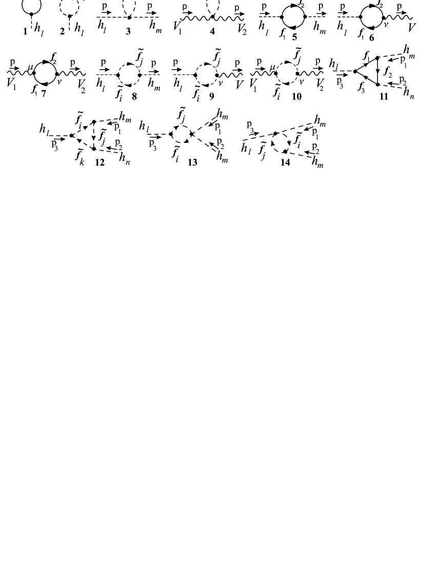
Figure 1: generic Yukawa one-loop diagrams contributing to the one-, two- and three-point Vertex Functions.

3.2 On-shell - renormalization of vertex function

For definition of counterterm $\delta\Gamma^{(n)}$ we shall use standard On-shell renormalization scheme [27]. Structure of counterterms is fixed by system of standard renormalization conditions for

• self-energies of gauge bosons $Z,\,W,\gamma$, and Higgs boson $A$;

• mixing energies $A-Z$,$\gamma-Z$;

• residue conditions for $A,\,\gamma$-bosons propagators;

• the renormalization of $\mathrm{tg}\beta$ in such a way that the relation $\mathrm{tg}\beta=v_{2}/v_{1}$ is valid for the one-loop Higgs minima;

• the tadpole conditions for vanishing renormalized tadpoles, i.e. the sum of the one-loop tadpole diagrams for $h^{0}$, $H^{0}$ and the corresponding tadpole counterterm is equal to zero.

Solving the received system of 11 linearized equations concerning initial counterterms, we have received the following results for counterterms of three-point Higgs Vertex functions:

$$\!\!\!\!\textstyle\delta\Gamma_{hhh}=\frac{3g_{2}M_{Z}^{2}}{4M_{W}^{2}}\left[\Big{(}-3M_{W}\Sigma_{A}^{\prime}(M_{A}^{2})+\frac{1}{M_{W}s_{w}^{2}}(1-2s_{w}^{2})\Sigma_{W}(M_{W}^{2})+\frac{M_{W}}{M_{Z}^{2}s_{w}^{2}}(-1+3s_{w}^{2})\times\right.$$

$$\!\!\!\!\textstyle\times\Sigma_{Z}(M_{Z}^{2})+M_{W}\Sigma_{\gamma}^{\prime}(0)-\frac{2s_{w}}{M_{Z}}\Sigma_{\gamma Z}(0)\Big{)}c_{2\alpha}s_{(\alpha+\beta)}+\frac{M_{W}}{2M_{Z}s_{2\beta}}\Sigma_{AZ}(M_{A}^{2})\Big{(}-s_{(\alpha-3\beta)}+$$

$$\!\!\!\!\left.\textstyle+3s_{(3\alpha-\beta)}-7s_{(\alpha+\beta)}+s_{(3(\alpha+\beta))}\Big{)}\right],$$

$$\!\!\!\!\textstyle\delta\Gamma_{hhH}=\frac{g_{2}M_{Z}^{2}}{4M_{W}^{2}}\left[\Big{(}-\frac{3}{2}M_{W}\Sigma_{A}^{\prime}(M_{A}^{2})-\frac{1}{2M_{W}s_{w}^{2}}(-1+2s_{w}^{2})\Sigma_{W}(M_{W}^{2})+\frac{M_{W}}{2M_{Z}^{2}s_{w}^{2}}(-1+3s_{w}^{2})\times\right.$$

$$\!\!\!\!\textstyle\times\Sigma_{Z}(M_{Z}^{2})+\frac{M_{W}}{2}\Sigma_{\gamma}^{\prime}(0)-\frac{s_{w}}{M_{Z}}\Sigma_{\gamma Z}(0)\Big{)}(c_{(\alpha-\beta)}-3c_{(3\alpha+\beta)})+\frac{M_{W}}{2M_{Z}s_{2\beta}}\Sigma_{AZ}(M_{A}^{2})\Big{(}c_{(\alpha-3\beta)}-$$

$$\!\!\!\!\textstyle\left.-9c_{(3\alpha-\beta)}+7c_{(\alpha+\beta)}-3c_{(3(\alpha+\beta))}\Big{)}\right],$$

$$\!\!\!\!\textstyle\delta\Gamma_{hHH}=\frac{g_{2}M_{Z}^{2}}{4M_{W}^{2}}\left[\Big{(}\frac{3}{2}M_{W}\Sigma_{A}^{\prime}(M_{A}^{2})+\frac{1}{2M_{W}s_{w}^{2}}(-1+2s_{w}^{2})\Sigma_{W}(M_{W}^{2})+\frac{M_{W}}{2M_{Z}^{2}s_{w}^{2}}(-1+3s_{w}^{2})\times\right.$$

$$\!\!\!\!\textstyle\times\Sigma_{Z}(M_{Z}^{2})+\frac{M_{W}}{2}\Sigma_{\gamma}^{\prime}(0)+\frac{s_{w}}{M_{Z}}\Sigma_{\gamma Z}(0)\Big{)}(s_{(\alpha-\beta)}+3s_{(3\alpha+\beta)})-\frac{M_{W}}{2M_{Z}s_{2\beta}}\Sigma_{AZ}(M_{A}^{2})\Big{(}s_{(\alpha-3\beta)}+$$

$$\!\!\!\!\textstyle\left.+9s_{(3\alpha-\beta)}+7s_{(\alpha+\beta)}+3s_{(3(\alpha+\beta))}\Big{)}\right],$$

$$\!\!\!\!\textstyle\delta\Gamma_{HHH}=\frac{3g_{2}M_{Z}^{2}}{4M_{W}^{2}}\left[\Big{(}-3M_{W}\Sigma_{A}^{\prime}(M_{A}^{2})+\frac{1}{M_{W}s_{w}^{2}}(1-2s_{w}^{2})\Sigma_{W}(M_{W}^{2})+\frac{M_{W}}{M_{Z}^{2}s_{w}^{2}}(-1+3s_{w}^{2})\times\right.$$

$$\!\!\!\!\textstyle\times\Sigma_{Z}(M_{Z}^{2})+M_{W}\Sigma_{\gamma}^{\prime}(0)-\frac{2s_{w}}{M_{Z}}\Sigma_{\gamma Z}(0)\Big{)}c_{2\alpha}c_{(\alpha+\beta)}+\frac{M_{W}}{2M_{Z}s_{2\beta}}\Sigma_{AZ}(M_{A}^{2})\Big{(}c_{(\alpha-3\beta)}+$$

$$\!\!\!\!\left.\textstyle+3c_{(3\alpha-\beta)}+7c_{(\alpha+\beta)}+c_{(3(\alpha+\beta))}\Big{)}\right].$$

In last system $s_{w}=\sin\theta_{w}$, $\theta_{w}$ – Weinberg angle.

3.3 Decay Amplitude calculation at one-loop level

Calculation of decay width at one-loop level is reduced to calculation of process amplitude $\mathcal{A}_{H\to hh}$, since one defines expression for decay width as

$$\Gamma(H\rightarrow hh)=\frac{\left|\mathcal{A}_{H\to hh}\right|^{2}}{32\pi M_{H}}\sqrt{1-\frac{4M_{h}^{2}}{M_{H}^{2}}},$$ (9)

where $M_{h},M_{H}$ – masses of $CP$-even Higgs physical states in the corresponding approximation, being real parts of the following equation roots:

$$\left[p^{2}-m^{2}_{h}+\hat{\Sigma}_{hh}(p^{2})\right]\left[p^{2}-m^{2}_{H}+\hat{\Sigma}_{HH}(p^{2})\right]-\left[\hat{\Sigma}_{hH}(p^{2})\right]^{2}=0.$$

For determination of $\mathcal{A}_{H\to hh}$ we shall make transition to basis of renormalized fields by means of $Z$-matrix

$$\begin{pmatrix}h\\ H\\ \end{pmatrix}\mapsto\begin{pmatrix}Z_{hh}^{\frac{1}{2}}&Z_{hH}^{\frac{1}{2}}\\ Z_{Hh}^{\frac{1}{2}}&Z_{HH}^{\frac{1}{2}}\\ \end{pmatrix}\begin{pmatrix}h_{R}\\ H_{R}\\ \end{pmatrix}$$

in lagrangian (4) in which are included Higgs self-couplings at one-loop level. Isolating the coefficient at product $h_{R}h_{R}H_{R}$, we derive expression for amplitude of process

$${\cal A}=Z^{\frac{1}{2}}_{HH}\left[Z^{\frac{1}{2}}_{hh}\right]^{2}\Gamma_{hhH}^{[I]}+2Z^{\frac{1}{2}}_{HH}Z^{\frac{1}{2}}_{hh}Z^{\frac{1}{2}}_{Hh}\Gamma_{hHH}^{[I]}+Z^{\frac{1}{2}}_{hH}\left[Z^{\frac{1}{2}}_{hh}\right]^{2}\Gamma_{hhh}^{[I]}.$$ (10)

Taking into account next on-shell condition: real part of residue from propagator in a pole should be equal to unit, it is possible to show, that $Z$-matrix elements are represented as follows:

$$\begin{array}[]{ll}Z^{\frac{1}{2}}_{hh}=1-\hat{\Sigma}\,^{\prime}_{hh}(M_{h}^{2}),&Z^{\frac{1}{2}}_{hH}=-\hat{\Sigma}_{hH}(M_{H}^{2})/(M_{H}^{2}-M_{h}^{2}),\\[5.69054pt] Z^{\frac{1}{2}}_{Hh}=-\hat{\Sigma}_{hH}(M_{h}^{2})/(M_{h}^{2}-M_{H}^{2}),&Z^{\frac{1}{2}}_{HH}=1-\hat{\Sigma}\,^{\prime}_{HH}(M_{H}^{2}).\end{array}$$

4 Numerical results and analysis

Let’s consider numerical results for self-couplings and decay width derived by scheme of calculation, presented in previous sections.

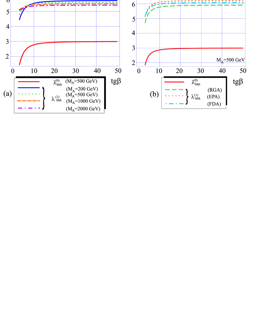
Figure 2: dependence from $\mathrm{tg}\beta$ of (a) new results for self-coupling $\lambda_{hhh}$ (in units $\lambda_{0}$); (b) RGA results [18, 19, 20], EPA results [21], FDA complete one-loop results [24, 25] for $A_{f}=1$ TeV, $\mu=0.5$ TeV, $M_{\tilde{Q}}=$ $M_{\tilde{U}}=$ $M_{\tilde{D}}=$ $M_{\tilde{L}}=$ $M_{\tilde{R}}=1$  TeV, $\sqrt{p_{3}^{2}}=(2M_{h}+10)$ GeV.

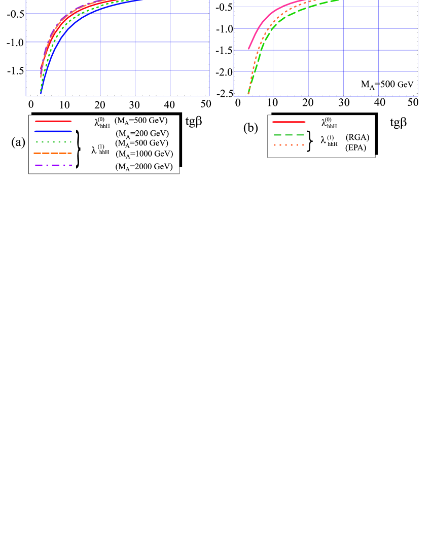
Figure 3: dependence from $\mathrm{tg}\beta$ of (a) new results for self-coupling $\lambda_{hhH}$ (in units $\lambda_{0}$); (b) RGA results [18, 19, 20], EPA results [21] for $A_{f}=1$ TeV, $\mu=0.5$ TeV, $M_{\tilde{Q}}=$ $M_{\tilde{U}}=$ $M_{\tilde{D}}=$ $M_{\tilde{L}}=$ $M_{\tilde{R}}=1$  TeV, $\sqrt{p_{3}^{2}}=(2M_{h}+10)$ GeV.

Dependence $\lambda_{hhh}$ (in units $\lambda_{0}=M_{Z}^{2}/v$) from $\mathrm{tg}\beta$ for four values of $M_{A}$ is represented on fig. 2.(a). Obviously, one-loop contribution essentially modifies tree-level result for any value $M_{A}$. The problem of significant corrections to the given self-coupling has been investigated in details in [23]; the exhaustive explanation to the specified phenomenon has been given. On fig. 2.(b) RGA results [18, 19, 20], EPA results [21], FDA complete one-loop results [24, 25] are shown. The new results are most consistent with RGA results. Difference between new results and FDA complete one-loop results [24, 25] is determined by non-leading one-loop corrections with virtual gauge bosons, Higgs bosons, chargino, neutralino (discrepancy is about $\leq 0.25\lambda_{0}$). All investigating Higgs self-couplings very weakly depend from $M_{A},\mu,A_{f},M_{S}$, therefore we will not demonstrate these dependencies.

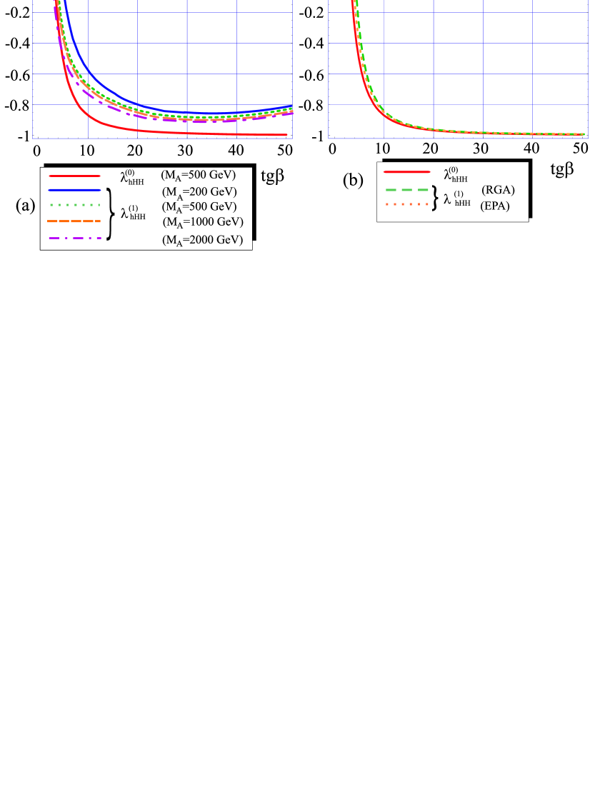
Figure 4: dependence from $\mathrm{tg}\beta$ of (a) new results for self-coupling $\lambda_{hHH}$ (in units $\lambda_{0}$); (b) RGA results [18, 19, 20], EPA results [21] for $A_{f}=1$ TeV, $\mu=0.5$ TeV, $M_{\tilde{Q}}=$ $M_{\tilde{U}}=$ $M_{\tilde{D}}=$ $M_{\tilde{L}}=$ $M_{\tilde{R}}=1$  TeV, $\sqrt{p_{3}^{2}}=(M_{h}+M_{H}+10)$ GeV.

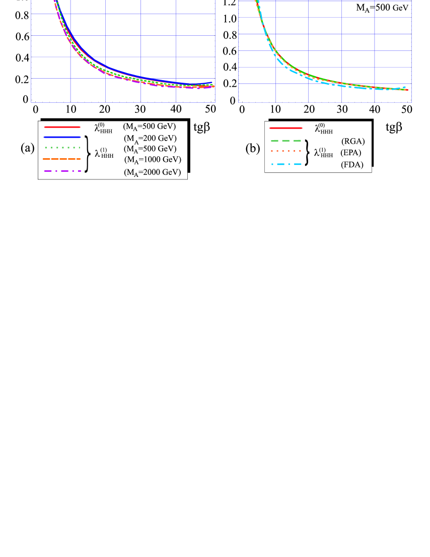
Figure 5: dependence from $\mathrm{tg}\beta$ of (a) new results for self-coupling $\lambda_{HHH}$ (in units $\lambda_{0}$); (b) RGA results [18, 19, 20], EPA results [21], FDA complete one-loop results [24, 25] for $A_{f}=1$ TeV, $\mu=0.5$ TeV, $M_{\tilde{Q}}=$ $M_{\tilde{U}}=$ $M_{\tilde{D}}=$ $M_{\tilde{L}}=$ $M_{\tilde{R}}=1$  TeV, $\sqrt{p_{3}^{2}}=(2M_{H}+10)$ GeV.

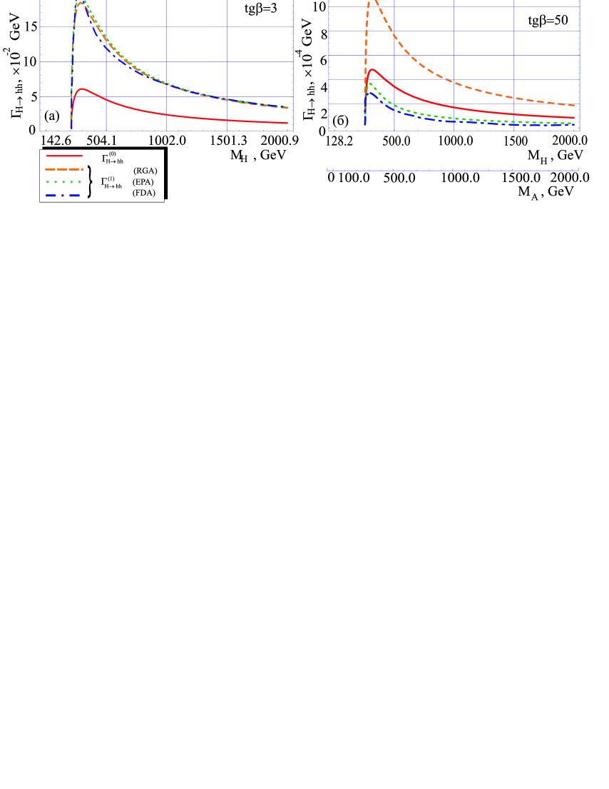
Figure 6: dependence of decay width from Higgs boson mass ($M_{h}$,$M_{H}$, $M_{A}$). for (a) $\mathrm{tg}\beta=3$, (b) $\mathrm{tg}\beta=50$ and $A_{f}=1$ TeV, $\mu=0.5$ TeV, $M_{\tilde{Q}}=$ $M_{\tilde{U}}=$ $M_{\tilde{D}}=$ $M_{\tilde{L}}=$ $M_{\tilde{R}}=1$ TeV.

On fig. 3(a)-(b) the curves of dependence $\lambda_{hhH}(\mathrm{tg}\beta)$ are demonstrated. Apparently, one-loop contributions in this case are not so large as in previous case. Maximal value of correction is reached for small values $M_{A}$ and $\mathrm{tg}\beta$. It is necessary to note, that our results in the specified area of values $M_{A}$ and $\mathrm{tg}\beta$ are less then values RGA and EPA results. This fact is caused by nonzero value $p_{3}$, impulse of virtual Higgs boson.

Fig. 4 demonstrates the curves of dependence $\lambda_{hHH}(\mathrm{tg}\beta)$, which are given in different perturbative approaches. Our curves testify to significant size of the corrections as against predecessors results. The reason for that – display of threshold effects. It is well known, correct description of observables near threshold of production is achieved only in Feynman diagram approach. Our results are derived at $\sqrt{p_{3}^{2}}=(M_{h}+M_{H}+10)$ GeV, that corresponds to threshold region. There is one more feature – at large $\mathrm{tg}\beta$ we can observe significant increase of Higgs self-coupling, calculated at one-loop level. This is a result of $b\tilde{b}$, $\tau\tilde{\tau}$ – loop corrections growth. The last fact is bright confirmation of necessity in the given one-loop contributions account.

As for one-loop corrections for self-couplings $\lambda_{HHH}$, that ones are small. Growth of loop corrections at large $\mathrm{tg}\beta$ and threshold effect are not shown almost, since calculation is carried out for more heavy particles.

The dependence of decay width $\Gamma(H\to hh)$ from mass of neutral Higgs boson(s) at various values $\mathrm{tg}\beta$ is submitted on fig. 6.(a)-(b). Fine agreement of different approaches results we can see at $\mathrm{tg}\beta=3$. The reason is obvious, dominating contributions into final result for decay width are $t\tilde{t}$ – corrections which are taken into account in all approaches. At $\mathrm{tg}\beta=50$ results EPA and FDA are close. Discrepancy is caused only by the account of $b\tilde{b}$, $\tau\tilde{\tau}$ - loop contributions in FDA.

Fig. 7.(a)-(f) demonstrates sensitivity areas of $\Gamma_{H\to hh}$ for fix limit value, represented in plane $\mathrm{tg}\beta-M_{A}$. It is necessary to note, that our results have ”more good” behaviour than outcomes of [26], since the region where $\Gamma(H\to hh)\geq 0.15$ (GeV) (in our results) lays in the interval of heavier $M_{A}$. It is more preferable case for recent experimental restrictions and theoretical scenarios.

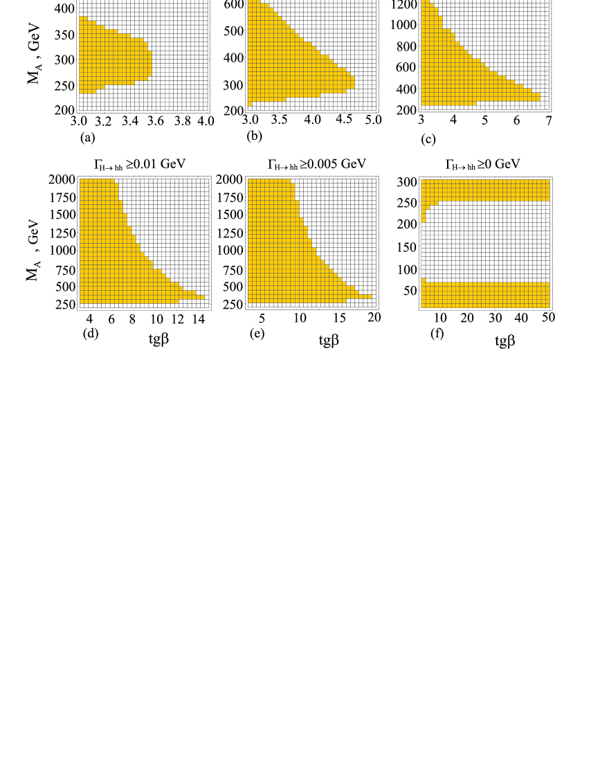
Figure 7: (a)-(f) sensitivity areas of $\Gamma_{H\to hh}$ for fix limit value, represented in plane $\mathrm{tg}\beta-M_{A}$, for $A_{f}=1$ TeV, $\mu=0.5$ TeV, $M_{\tilde{Q}}=M_{\tilde{U}}=M_{\tilde{D}}=M_{\tilde{L}}=M_{\tilde{R}}=1$  TeV.

5 Conclusions

Thus dependencies of Higgs-self couplings $\lambda_{hhh}$, $\lambda_{hhH}$, $\lambda_{hHH}$, $\lambda_{HHH}$ and decay width $\Gamma(H\to hh)$ from $\mathrm{tg}\beta$, $M_{A}$ have been analysed in present work. It has been shown, that one-loop results can essentially differ from tree-level ones. Applying for the precision comparative analysis of theoretical and experimental results with goal of self-couplings determination, it is necessary to use at least one-loop approximation. Last fact becomes a necessary condition of Higgs potential reconstruction and experimental confirmation of Higgs mechanism realization in nature.

References

- [1] Goldstone J. Field theories with ”superconductor” solutions // Nuovo Cimento. 1961. V. 19. P. 154-164.
- [2] Nambu Y., Jona-Lasinio G. Dynamical model of elementary particles based on an analogy with superconductivity. I // Phys. Rev. 1961. V. 122. P. 345-358.
- [3] Goldstone J., Salam A., Weinberg S. Broken symmetries // Phys. Rev. 1962. V. 127. P. 965-970.
- [4] Higgs P.W. Broken symmetries, massless particles and gauge fields // Phys. Lett. 1964. V. 12. P. 132-133.
- [5] Higgs P.W. Broken symmetries and the masses of gauge bosons // Phys. Rev. Lett. 1964. V. 13. P. 508-509.
- [6] Higgs P.W. Spontaneous symmetry breakdown without massless bosons // Phys. Rev. 1966. V. 145. P. 1156-1163.
- [7] R. Brout, E. Englert Broken symmetry and the mass of gauge vector mesons // Phys. Rev. Lett. 1964. V. 13. P. 321-322.
- [8] Guralnik G.S., Hagen C.R., Kibble T.W.B. Global conservation laws and massless particles // Phys. Rev. Lett. 1964. V. 13. P. 585-587.
- [9] Kibble T.W.B. Symmetry breaking in nonabelian gauge theories // Phys. Rev. 1967. V. 155. P. 1554-1561.
- [10] Zerwas P.M. Physics with an e+ e- linear collider at high luminosity // Eprint:hep-ph/0003221. 26pp.
- [11] Djouadi A., Haber H. E., Zerwas P. M. Multiple production of MSSM neutral higgs bosons at high-energy e+ e- colliders // Phys. Lett. B 1996. V. 375. P. 203-212.
- [12] Djouadi A., Kilian W., Mühlleitner M. and Zerwas P.M. Testing Higgs selfcouplings at e+ e- linear colliders // Eur. Phys. J. 1999. C 10. P. 27-43.
- [13] Djouadi A., Kilian W., Mühlleitner M. and Zerwas P.M. Production of neutral higgs boson pairs at LHC // Eur. Phys. J. 1999. C 10. P. 45-49.
- [14] Osland P., Pandita P. N. Measuring the trilinear couplings of MSSM neutral higgs bosons at high-energy e+ e- colliders // Phys. Rev. 1999. D V. 59. P. 055013. 18pp; Measuring trilinear Higgs couplings in the MSSM // E-print: hep-ph/9902270. 12pp; Multiple Higgs production and measurement of Higgs trilinear couplings in the MSSM // E-print: hep-ph/9911295. 12pp.
- [15] Djouadi A., Kalinowski J. and Zerwas P.M. Two and three-body decay modes of SUSY Higgs particles. // Z. Phys. 1996. C 70. P. 435-448.
- [16] Djouadi A., Kalinowski J. and Zerwas P.M. Exploring the SUSY Higgs sector at e+ e- linear colliders: A Synopsis // Z. Phys. 1993. C 57 P. 569-584.
- [17] Haber H.E. and Hempfling R. Can the mass of the lightest Higgs boson of the minimal supersymmetric model be larger than ? // Phys. Rev. Lett. 1991. V. 66. P. 1815-1818.
- [18] Haber H.E., Hempfling R. Nir Y. The decay in the minimal supersymmetric model // Phys. Rev. D 1992. V. 46. P. 3015-3024.
- [19] Ellis J., Ridolfi G. and Zwirner F. Radiative corrections to the masses of supersymmetric Higgs bosons // Phys. Lett. B 1991. V. 257. P. 83-91.
- [20] Okada Y., Yamaguchi M. and Yanagida T. Upper bound of the lightest Higgs boson mass in the minimal supersymmetric standard model // Prog. Theor. Phys. 1991. V. 85. P. 1-6.
- [21] Barger V., Berger M. S., Stange A. L. and Phillips R. J. N. Supersymmetric higgs boson hadroproduction and decays including radiative corrections //Phys. Rev. D 1992. V. 45. P. 4128-4147;
- [22] Kunszt Z. and Zwirner F. Testing the Higgs sector of the minimal supersymmetric standard model at large hadron colliders // Nucl. Phys. B 1992. V. 385. P. 3-75.
- [23] Hollik W., Penaranda S. Yukawa coupling quantum corrections to the selfcouplings of the lightest MSSM Higgs boson //Eur. Phys. J. 2002. C 23. P. 163-172.
- [24] Dolgopolov M.V., Philippov Yu.P. The trilinear neutral Higgs self-couplings in the MSSM. Complete one-loop analysis // Vestnik of Samara State University / Samara, ”Samara University”, 2-nd special realise 2003. P.87-95; hep-ph/0310263, 2003. 6pp.
- [25] Dolgopolov M.V., Philippov Yu.P. Vertex functions of the three-partial interaction of Higgs bosons , in MSSM: one-loop analysis // Yad. Fiz. 2004. V.67. 3. P. 609-613.
- [26] Brignole A., Zwirner F. Radiative corrections to the decay in the minimal supersymmetric standard model // Phys. Lett. B 1993. V. 299. P. 72-82.
- [27] Dabelstein A. The one loop renormalization of the MSSM higgs sector and its application to the neutral scalar higgs masses // Z. Phys. 1995. C 67. P. 495-512.
- [28] J. F. Gunion, H. E. Haber, G. Kane, and S. Dawson, The Higgs Hunter’s Guide (Addison-Wesley, 1990).
- [29] Brignole A. Radiative corrections to the supersymmetric charged Higgs boson mass // Phys. Lett. B 1992. V. 277. P. 313-323.
- [30] Brignole A. Radiative corrections to the supersymmetric neutral Higgs boson masses // Phys. Lett. B 1992. V. 281. P. 284-294.