Mass Determination in Cascade Decays Using Shape Formulas

Abstract

In SUSY scenarios with invisible LSP, sparticle masses can be determined from fits to the endpoints of invariant mass distributions. Here we discuss possible improvements by using the shapes of the distributions. Positive results are found for multiple-minima situations and for mass regions where the endpoints do not contain sufficient information to obtain the masses.

1 Introduction

In R-parity conserving supersymmetric models sparticles are produced in pairs at the collision point, then decay in cascades, resulting in a number of Standard Model particles as well as two Lightest Supersymmetric Particles (LSPs), one for each primary sparticle. If the LSPs leave the detector without a trace, as is the case in most scenarios of this type, the event cannot be fully reconstructed. This in turn prevents a direct measurement of the sparticle masses from mass peaks. The foreseen way to obtain these masses in such scenarios, is through endpoint measurements of invariant mass distributions Hinchliffe:1996iu ; Bachacou:1999zb ; Allanach:2000kt ; Lester:2001zx ; Gjelsten:2004ki ; Weiglein:2004hn ; Gjelsten:2005aw . Particularly suited is the cascade decay ${\tilde{q}_{L}}\to{\tilde{\chi}^{0}_{2}}q\to{\tilde{l}_{R}}{l_{\rm n}}q\to{\tilde{\chi}^{0}_{1}}{l_{\rm f}}{l_{\rm n}}q$ which for a large share of SUSY models and parameters is kinematically allowed and appears at a rate sufficient for study. Four invariant mass distributions can be constructed from the visible decay products, $m_{ll}$, $m_{qll}$, $m_{ql({\rm high})}$ and $m_{ql({\rm low})}$.

Once the endpoints have been measured, the masses can be found. However, measuring an endpoint is not trivial. A fit must be made to the edge region of the distribution. Such a fit necessarily involves a signal and a background hypothesis. If these are not in good correspondence with the true shapes, it is expected that the endpoint fitting may introduce large systematic uncertainties. While a straight-line hypothesis sometimes performs well, the fact that each distribution can take on a large variety of shapes Gjelsten:2004ki ; Gjelsten:2005aw really is a limiting factor, especially since a mismeasurement of an endpoint by 10 GeV can easily multiply to 40 GeV in the resulting masses. Without an appropriate signal hypothesis the endpoint method is incomplete. The many studies undertaken so far reflect this in that they have mainly focused on determining the statistical error, which can be fairly well estimated by a straight line, putting off the systematics of the fitting procedure for later investigations. With the recent advent of an analytic description of the shapes of these mass distributions Miller:2005zp , the time for such investigations has come closer.

2 Masses from shapes

The completion of the endpoint method requires formulas for the edge-region part of the distributions expressed by the endpoints. The shape formulas are however written in terms of the sparticle masses. Fitting the distributions gives the masses directly without any recourse to the endpoints. The considerable difference in approach asks for a comparison between the two methods. We here investigate the matter for the mSUGRA point SPS 1a Allanach:2002nj . In order for the characteristics of the methods to easily shine through, we make a simple comparison, with no background included, and no detector effects. The comparison is based on histograms generated randomly from the shape formulas taken from Miller:2005zp convoluted with a gaussian of width 2 GeV for $m_{ll}$ and 10 GeV for the other distributions. The selected procedure and numbers mimic the effect of sparticle widths, initial and final-state radiation, detector effects etc. The same procedure is also invoked for the shape-fitting process. The normalisation of the histograms corresponds roughly to the ultimate statistics expected for an LHC experiment.

	Nominal	Fitted	Error	Inflated error
$m^{\rm max}_{ll}$	77.07	77.13	0.04	0.04
$m^{\rm max}_{ql({\rm high})}$	375.8	378.9	0.4	1.2
$m^{\rm max}_{ql({\rm low})}$	298.5	304.2	0.8	2.4
$m^{\rm max}_{qll}$	425.9	432.3	0.3	0.9

Table 1: Endpoint values and errors [in GeV] for SPS 1a.

Endpoint method

For the endpoint analysis a straight-line fit is used to obtain the statistical uncertainty. Table 1 shows the nominal values together with the fitted values and the errors obtained. A second set of errors, three times the statistical ones, except for $m^{\rm max}_{ll}$, is included to give a slightly more realistic situation. The discrepancy between the nominal and the fitted endpoints reminds us of the problem with endpoint fitting.

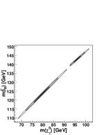
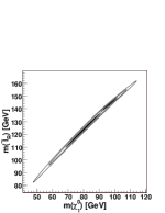
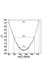
Figure 1: SPS 1a comparison. Left (Middle): endpoint method for the first (second) set or errors. Two minima are found, the correct one situated at ${m_{\tilde{\chi}^{0}_{1}}}=96$ GeV, the false at ${m_{\tilde{\chi}^{0}_{1}}}=80$ GeV. Right: shape fit to the same distributions. The false minimum is not present.

Figure 1 (left and middle) shows the resulting 1, 2 and 3$\sigma$ contours in the ${m_{\tilde{\chi}^{0}_{1}}}$–${m_{\tilde{l}_{R}}}$ plane for the two sets of errors. The nominal endpoint values are used, not the fitted ones. From these figures the main characteristics of the endpoint method are apparent: the occurrence of multiple solutions Gjelsten:2004ki ; Gjelsten:2005sv and strong mass correlation reflecting the fact that mass differences are accurately determined while the overall scale only poorly so.

Shape method

Since the background is expected to be more prominent for lower invariant masses, only the higher part of the distributions are used in the shape fit. The result of the fit is given by the $\chi^{2}$-function in Fig. 1 (right). Notice that the false solution is absent. The shape difference for the two mass sets is apparently sufficient to discriminate between them. Whether or not this situation holds for a more realistic analysis remains to be seen. The shape difference between these two points is below mSUGRA average Raklev2006 . The precision on the overall mass scale returned by the shape fit is roughly as for the endpoint approach using the second error set, except for the false solution present in the endpoint case which stretches to very low masses. Finally it is found that also for the shape fitting method the resulting masses are very correlated, constraining mass differences much more than masses. More study is however needed to compare the degree of correlation to that obtained from the endpoint method.

3 When endpoints are not enough

In some regions of mass space the four endpoints are no longer linearly independent due to $(m^{\rm max}_{qll})^{2}=(m^{\rm max}_{ll})^{2}+(m^{\rm max}_{ql({\rm high})})^{2}$. When this happens, which is for regions (2,3), (3,1) and (3,2) in the notation of Gjelsten:2004ki , curves exist in the four-dimensional mass space on which all mass points produce the same endpoints. In region (3,2) the curve is given by

$${m_{\tilde{l}_{R}}^{2}}=\frac{{m_{\tilde{\chi}^{0}_{1}}^{2}}}{2-A},\phantom{ee}{m_{\tilde{\chi}^{0}_{2}}^{2}}={m_{\tilde{l}_{R}}^{2}}+\frac{(m^{\rm max}_{ll})^{2}}{A-1},\phantom{ee}{m_{\tilde{q}_{L}}^{2}}={m_{\tilde{l}_{R}}^{2}}+\frac{(m^{\rm max}_{qll})^{2}}{A-1},\phantom{ee}A=\left(\frac{m^{\rm max}_{ql({\rm high})}}{m^{\rm max}_{ql({\rm low})}}\right)^{2}$$ (1)

From one mass set new mass sets on the curve can be generated by keeping the endpoints fixed, then changing ${m_{\tilde{\chi}^{0}_{1}}}$ and calculating the other masses.

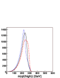
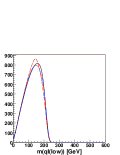
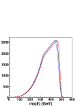
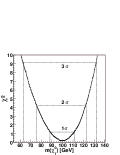
Figure 2: Left to right: $m_{ql({\rm high})}$, $m_{ql({\rm low})}$ and $m_{qll}$ for three points in region (3,2), all having the same endpoints, but different distributions. Right: $\chi^{2}$-function from fitting the shapes has minimum at the correct ${m_{\tilde{\chi}^{0}_{1}}}$. Only smearing is applied, no statistical fluctuations, therefore $\chi^{2}_{\min}=0$.

Under these circumstances four endpoint measurements do not impose sufficient constraints to obtain the masses. Extra information is however available from the shapes. Figure 2 (three leftmost) shows the relevant gaussian-convoluted (width 10 GeV) mass distributions for the mass set $({m_{\tilde{\chi}^{0}_{1}}},{m_{\tilde{l}_{R}}},{m_{\tilde{\chi}^{0}_{2}}},{m_{\tilde{q}_{L}}})=(100,300,500,600)$ GeV (black, solid), and two sets on the line (1) defined by increasing (blue, dotted) and decreasing (red, dashed) ${m_{\tilde{\chi}^{0}_{1}}}$ by 30 GeV. While the endpoints are the same, the shapes are seen to differ. (The $m_{ll}$ distribution is not shown as its shape is always the same.)

Based on the distributions of the original mass set (${m_{\tilde{\chi}^{0}_{1}}}=100$ GeV, black solid), histograms are generated, assuming a similar number of events as for the previous SPS 1a investigations. Figure 2 (right) shows the $\chi^{2}$ function from a shape fit to these distributions. The histograms contain no statistical fluctuations, which is why the minimum is at $\chi^{2}=0$. Adding statistical fluctuations will lift $\chi^{2}_{\min}$ from zero, but the conclusion stays the same: A clear minimum is found for the correct masses in this region where the endpoints alone can not bring the masses.

4 Conclusion

We have investigated the use of shape formulas to obtain the sparticle masses in scenarios where the LSP is undetected. Comparison with the standard endpoint method was made for the mSUGRA point SPS 1a. The extra solution at ${m_{\tilde{\chi}^{0}_{1}}}=80$ GeV which is returned by the endpoint inversion, is absent in the shape-fitting results. The strong correlation in the resulting masses remains: Mass differences are accurately determined while the overall mass scale has larger uncertainties. It was furthermore shown that the use of shapes allows for masses to be determined in regions of mass space where the endpoints alone do not suffice due to linear interdependence. In conclusion, the use of shapes to determine masses constitute a very promising approach. More study is needed. It is particularly important to understand what impact the distortion of the invariant mass distributions, particularly from selection cuts and various backgrounds, will have on the proposed shape fitting technique.

References

- (1) I. Hinchliffe, F. E. Paige, M. D. Shapiro, J. Soderqvist and W. Yao, Phys. Rev. D 55 (1997) 5520 [arXiv:hep-ph/9610544].
- (2) H. Bachacou, I. Hinchliffe and F. E. Paige, Phys. Rev. D 62 (2000) 015009 [arXiv:hep-ph/9907518].
- (3) B. C. Allanach, C. G. Lester, M. A. Parker and B. R. Webber, JHEP 0009 (2000) 004 [arXiv:hep-ph/0007009].
- (4) C. G. Lester, CERN-THESIS-2004-003.
- (5) B. K. Gjelsten, D. J. Miller and P. Osland, JHEP 0412 (2004) 003 [arXiv:hep-ph/0410303].
- (6) G. Weiglein et al. [LHC/LC Study Group], Phys. Rept. 426 (2006) 47 [arXiv:hep-ph/0410364].
- (7) B. K. Gjelsten, D. J. Miller and P. Osland, JHEP 0506 (2005) 015 [arXiv:hep-ph/0501033].
- (8) D. J. Miller, P. Osland and A. R. Raklev, JHEP 0603 (2006) 034 [arXiv:hep-ph/0510356].
- (9) B. C. Allanach et al., in Proc. of the APS/DPF/DPB Summer Study on the Future of Particle Physics (Snowmass 2001) ed. N. Graf, Eur. Phys. J. C 25 (2002) 113 [eConf C010630 (2001) P125] [arXiv:hep-ph/0202233].
- (10) B. K. Gjelsten, D. J. Miller and P. Osland, arXiv:hep-ph/0507232; arXiv:hep-ph/0511008.
- (11) B. K. Gjelsten, D. J. Miller, P. Osland, A. R. Raklev, to appear in Proc. of the XXXIII International Conference on High Energy Physics (ICHEP’06), Moscow, Russia, 26 July–2 August 2006 [arXiv:hep-ph/0611080].