Heavy Quark Mass Effects in Deep Inelastic Scattering and Global QCD Analysis

Abstract:

A new implementation of the general PQCD formalism of Collins, including heavy quark mass effects, is described. Important features that contribute to the accuracy and efficiency of the calculation of both neutral current (NC) and charged current (CC) processess are explicitly discussed. This new implementation is applied to the global analysis of the full HERA I data sets on NC and CC cross sections, with correlated systematic errors, in conjunction with the usual fixed-target and hadron collider data sets. By using a variety of parametrizations to explore the parton parameter space, robust new parton distribution function (PDF) sets (CTEQ6.5) are obtained. The new quark distributions are consistently higher in the region $x\sim 10^{-3}$ than previous ones, with important implications on hadron collider phenomenology, especially at the LHC. The uncertainties of the parton distributions are reassessed and are compared to the previous ones. A new set of CTEQ6.5 eigenvector PDFs that encapsulates these uncertainties is also presented.

1 Introduction

Global QCD analysis of the parton structure of the nucleon has made significant progress in recent years. However, there remain many gaps in our knowledge of the parton distribution functions (PDFs), especially with regard to the strange, charm and bottom degrees of freedom. The uncertainties of the PDFs remain large in both the very small-$x$ and the large-$x$ regions—in general for all flavors, but particularly for the gluon.  Uncertainties due to the input PDFs will be one of the dominant sources of uncertainty in some precision measurements (such as the $W$ mass) [1], as well as in studying signals and backgrounds for New Physics searches at the Fermilab Tevatron and the CERN Large Hadron Collider (LHC). Thus, improving the accuracy of the global QCD analysis of PDFs is a high priority task for High Energy Physics.

With the accumulation of extensive precision deep inelastic scattering (DIS) cross section measurements of both the neutral current (NC) and charged current (CC) processes at HERA I (and even more precise data from HERA II to come soon), it is necessary to employ reliable theoretical calculations that match the accuracy of the best data in the global analysis.  In the perturbative QCD framework (PQCD), this requires, among other things, a proper treatment of the heavy quark mass parameters. There are many aspects to a proper treatment of general mass effects, involving both dynamics (consistent factorization in PQCD, with quark massess) and kinematics (physical phase space constraints with heavy flavor masses that are not satisfied by the simplest implementation of the zero-mass parton model formula). Some aspects of these considerations have been applied in existing work on global QCD analysis; however, in most cases, not all relevant effects have been consistently taken into account.

In this paper, we present a systematic discussion of the relevant physics issues, and provide a new implementation of the general formalism for all DIS processes in a unified framework (Sec. 2). We show the magnitude of the mass effects, compared to the conventional zero-mass (ZM) parton formalism (Sec. 3). We then apply this simple implementation of the general mass formalism to a precise global analysis of PDFs, including the full HERA I cross section data sets for both NC and CC processes, and taking into account all available correlated systematic errors (Sec. 4). We investigate in some depth the parametrization dependence of the global analysis, assess the uncertainties of the PDFs in the new analysis, and compare the new results with those of CTEQ6.1 [2] (which was based on the ZM parton formalism) and other current PDFs [3] (Sec. 5). The results, designated as CTEQ6.5 PDFs, have important implications for hadron collider phenomenology at the Tevatron and the LHC. Finally, we summarize our main results, discuss their limitations, and mention the challenges ahead (Sec. 7). Some preliminary results of this investigation have been presented at the DIS2006 Workshop [4].

2 General Mass PQCD:
Formalism and Implementation

The quark-parton picture is based on the factorization theorem of PQCD. The conventional proof of the factorization theorem proceeds from the zero-mass limit for all the partons—a good approximation at energy scales (generically designated by $Q$) far above all quark mass thresholds (designated by $M_{i}$). This clearly does not hold when $Q/M_{i}$ is of order 1. It has been recognized since the mid-1980’s that a consistent treatment of heavy quarks in PQCD over the full energy range from $Q\lesssim M_{i}$ to $Q\gg M_{i}$ can be formulated [5]. (This is most clearly seen in the CWZ renormalization scheme [6].) The basic physics ideas were further developed in [7]; this approach has become generally known as the ACOT scheme. In 1998, Collins gave a general proof (order-by-order to all orders of perturbation theory) of the factorization theorem that is valid for non-zero quark masses [8]. The resulting theoretical framework is conceptually simple: it represents a straightforward generalization of the conventional zero-mass (ZM) modified minimal subtraction ($\overline{MS}$) formalism. This general mass (GM) formalism is what we shall adopt.

The implementation of the general mass formalism requires attention to a number of details, both kinematical and dynamical, that can affect the accuracy of the calculation. Physical considerations are important to ensure that the right choices are made between perturbatively equivalent alternatives that may produce noticeable differences in practical applications. We now systematically describe these considerations, and spell out the specifics of the new implementation used in our study.  For simplicity, we shall often focus on the charm quark, and consider the relevant issues relating to the calculation of structure functions at a renormalization and factorization scale $\mu$ (usually chosen to be equal to $Q$) in the neighborhood of the charm mass $M_{c}$. The same considerations apply to the other heavy quarks, and to the calculation of cross sections.

2.1 The Factorization Formula

Let the total inclusive differential cross section for a general DIS scattering process be written as

$$\frac{d^{2}\sigma}{dxdy}=N\sum_{\lambda}\,L_{\lambda}(x,y)F^{\lambda}(x,Q)$$ (1)

where $F^{\lambda}(x,Q)$ are structure functions representing the forward Compton amplitudes for the exchanged vector bosons on the target nucleon, $L_{\lambda}(x,y)$ are kinematic factors originating from the (calculable) lepton scattering vertices, and $N$ is an overall factor dependent on the particular process. We follow the notation of Ref. [9], from which detailed formulas for the above factors can be found. The PQCD factorization theorem for the structure functions has the general form

$$F^{\lambda}(x,Q^{2})=\sum_{a}f^{a}\otimes\widehat{\omega}_{a}^{\lambda}=\sum_{a}\int_{\zeta}^{1}{\frac{d\xi}{\xi}}\ f^{a}(\xi,\mu)\ \widehat{\omega}_{a}^{\lambda}\left(\frac{x}{\xi},\frac{Q}{\mu},\frac{M_{i}}{\mu},\alpha_{s}(\mu)\right).$$ (2)

Here, the summation is over the active parton flavor label $a$, $f^{a}(x,\mu)$ are the parton distributions at the factorization scale $\mu$, $\widehat{\omega}_{a}^{\lambda}$ are the Wilson coefficients (or hard-scattering amplitudes) that can be calculated order-by-order in perturbation theory, and we have implicitly set the renormalization and factorization scales to be the same. The lower limit of the convolution integral $\zeta$ is usually taken to be $x=Q^{2}/2q\cdot p$—the Bjorken $x$—in the conventional ZM formalism; but this choice needs to be re-considered when the Wilson coefficients include heavy quark mass effects, as we shall do in Sec. 2.4 below. In most applications, it is convenient to choose $\mu=Q$; but there are circumstances in which a different choice becomes useful. For DIS at order $\alpha_{s}$ and beyond, the results are known to be quite insensitive to the choice of $\mu$.

2.2 The (Scheme-dependent) Parton Distributions and Summation over Parton Flavors

The summation $\sum_{a}$ over “parton flavor” label $a$ in the factorization formula, Eq. (2), is determined by the factorization scheme chosen to define the Parton Distributions $f_{a}(x,\mu)$.

In the fixed flavor number scheme (FFNS), one sums over $a=g,u,\bar{u},d,\bar{d},...$ up to $n_{f}$ flavors of quarks, where $n_{f}$ is held at a fixed value ($3,4,...$). For a given $n_{f}$ (say $n_{f}=3)$, the $n_{f}$-FFNS has only a limited range of applicability, since, at order $m$ of the perturbative expansion, the Wilson coefficients contain logarithm terms of the form $\alpha_{s}^{m}\ln^{m}(Q/M_{i})$ for $i>n_{f}$, which is not infrared safe as $Q$ becomes large compared to the renormalized mass of the heavy quark $M_{i}$ (e.g. $M_{c,b}$, in the $n_{f}=3$ example).

The more general variable flavor number scheme (VFNS), as defined in Collins’ general framework [5, 8], is really a composite scheme: it consists of a series of FFNS’s matched at conveniently chosen match points $\mu_{i}$, one for each of the heavy quark thresholds. At $\mu_{i}$, the $n_{f}$-flavor scheme is matched to the $(n_{f}+1)$-flavor scheme by a set of perturbatively calculable finite renormalizations of the coupling parameter $\alpha_{s}$, the mass parameters $\left\{M_{i}\right\}$, and the parton distribution functions $\left\{f^{a}\right\}$. The matching scale $\mu_{i}$ can, in principle, be chosen to be any value, as long as it is of the order of $M_{i}$. In practice, it is usually chosen to be $\mu_{i}=M_{i}$, since it has been known that, in the commonly used (VFNS) $\overline{MS}$ scheme, all the renormalized quantities mentioned above are continuous at this point up to NLO in the perturbative expansion [5]. Normally, when the VFNS is applied at a factorization scale $\mu$ that lies in the interval ($\mu_{n_{f}},\mu_{n_{f}+1}$), the $n_{f}$-flavor scheme is used. Thus the number of active parton flavors depends on the scale $\mu$—henceforth denoted by $n_{f}(\mu)$—and it increases by one when $\mu$ crosses the threshold $\mu_{i+1}$ from below.

PQCD in the VFNS is free of large logarithms of the kind mentioned above for the FFNS—it is infrared safe, and hence remains reliable, at all scales $\mu$ ($\sim Q$) $\gg\Lambda_{QCD}$. In this scheme, the range of summation over “$a$” in the factorization formula, Eq. (2), is $0,1,...,n_{f}(\mu)$, where $0$ represents the gluon, $1$ represents $u$ and $\bar{u}$, etc.

Our implementation of the general mass formalism includes both FFNS and VFNS. In practice, however, for reasons already mentioned, we shall mostly use the VFNS. The definition of parton distributions in the scheme described above is exactly the same as that of previous CTEQ PDFs, all being based on [5]. (It is also shared, essentially, by most global analysis groups, e.g. MRST [10].) The improvements of the formalism over previous analyses reside in the consistent and systematic treatment of mass effects in the Wilson coefficients and in the phase space integral of Eq. (2) that we shall now describe and clarify.

2.3 The Summation over (Physical) Final-state Flavors

For total inclusive structure functions, the factorization formula, Eq. (2), contains an implicit summation over all possible quark flavors in the final state. One can write,

$$\hat{\omega}_{a}=\sum_{b}\hat{\omega}_{a}^{b}$$ (3)

where “$b$” denotes final state flavors, and $\hat{\omega}_{a}^{b}$ is the perturbatively calculable hard cross section for an incoming parton “$a$” to produce a final state containing flavor “$b$ ”. (Cf. the Feynman diagrams contributing to the calculation of the hard cross section in Sec. 2.5 below. A caveat on the definition of $\hat{\omega}_{a}^{b}$, is described in Sec. 2.6.)

It is important to emphasize that “$b$” labels quark flavors that can be produced physically in the final state; it is not a parton label in the sense of initial-state parton flavors described in the previous subsection. The latter (labelled $a$) is a theoretical construct and scheme-dependent (e.g. it is fixed at three for the 3-flavor scheme); whereas the final-state sum (over $b$) is over all flavors that can be physically produced. The initial state parton “$a$” does not have to be on the mass-shell. But the final state particles “$b$” should be on-mass-shell in order to satisfy the correct kinematic constraints and yield physically meaningful results. Thus, in implementing the summation over final states, the most relevant scale is $W$—the CM energy of the virtual Compton process—in contrast to the scale $Q$ that controls the initial state summation over parton flavors (see next subsection).

The distinction between the two summations is absent in the simplest implementation of the conventional (i.e., textbook) zero-mass parton formalism: if all quark masses are set to zero to begin with, then all flavors can be produced in the final state.  This distinction becomes blurred in a zero-mass (ZM) VFNS—the one commonly used in the literature (including previous CTEQ analyses)—where the number of effective parton flavors is incremented as the scale parameter $\mu$ crosses a heavy quark threshold, but other kinematic and dynamic mass effects are omitted.  Thus, the implementation of the ZM VFNS by different groups can be different, depending on how the final-state summation is carried out. This detail is usually not spelled out in the relevant papers.

It should be obvious that, in a proper implementation of the general mass (GM) formalism, the distinction between the initial-state and final-state summation must be unambiguously, and correctly, observed.  For instance, even in the 3-flavor regime (when $c$ and $b$ quarks are not counted as partons), the charm and bottom flavors still need to be counted in the final state—at LO via $W^{+}+d/s\rightarrow c$ or $W^{-}+u/c\rightarrow b$, and at NLO via the gluon-fusion processes such as $W^{+}+g\rightarrow\bar{s}+c$ or $\gamma+g\rightarrow c\bar{c}\,(b\bar{b})$, provided there is enough CM energy to produce these particles.

This issue immediately suggests that one must also give careful consideration to the proper treatment of the integral over the final-state phase space and other kinematical effects in the problem.

2.4 Kinematic Constraints and Rescaling

Once mass effects are taken into account, kinematic constraints have a significant impact on the numerical results of the calculation; in fact, they represent the dominant factor in the threshold regions of the phase space.  In DIS, with heavy flavor produced in the final state, the simplest kinematic constraint that comes to mind is

$$W-M_{N}>\sum_{f}~{}M_{f}$$ (4)

where $W$ is the CM energy of the vector-boson–nucleon scattering process, $M_{N}$ is the nucleon mass, and the right-hand side is the sum of all masses in the final state. Since $W$ is related to the familiar kinematic variables ($x,Q$) by $W^{2}-M_{N}^{2}=Q^{2}(1-x)/x$, this constraint can be imposed by a step function $\theta(W-M_{N}-\sum_{f}M_{f})$ condition on the right-hand side of Eq. (2), irrespective of how, or whether, mass effects are incorporated in the convolution integral. Although that simple approach would represent an improvement over ignoring the kinematic constraint Eq. (4), it is too crude, and can lead to undesirable discontinuities.

A much better physically motivated approach is based on the idea of rescaling. The simplest example is given by charm production in the LO CC process $W+s\rightarrow c$. It is well-known that, when the final state charm quark is put on the mass shell, the appropriate momentum fraction variable for the incoming strange parton, $\chi$ in Eq. (2), is not the Bjorken $x$, but rather $\chi=x(1+M_{c}^{2}/Q^{2})$ [11]. This is commonly called the rescaling variable.

The generalization of this idea to the more prevalent case of NC processes, say $\gamma/Z+c\rightarrow c$ (or any other heavy quark), took a long time to emerge [12], because this partonic process implies the existence of a hidden heavy particle—the $\bar{c}$—in the target fragment. The key observation was, heavy objects buried in the target fragment are still a part of the final state, hence must be included in the phase space constraint, Eq. (4). Taking this effect into account, and expanding to the more general case of $\gamma/Z+c\rightarrow c+X$, where $X$ contains only light particles, it was proposed that the convolution integral in Eq. (2) should be over the momentum fraction range $\chi_{c}<\xi<1$, where

$$\chi_{c}=x\left(1+\frac{4M_{c}^{2}}{Q^{2}}\right)\ \ .$$ (5)

In the most general case where there are any number of heavy particles in the final state, the corresponding variable is (cf. Eq. (4))

$$\chi=x\left(1+\frac{\left(\Sigma_{f}~{}M_{f}\right)^{2}}{Q^{2}}\right)\ \ .$$ (6)

This rescaling prescription has been referred to as ACOT$\chi$ in the recent literature [12, 10].

Fig. 1 helps to visualize the physical effects of rescaling for charm production in NC DIS.

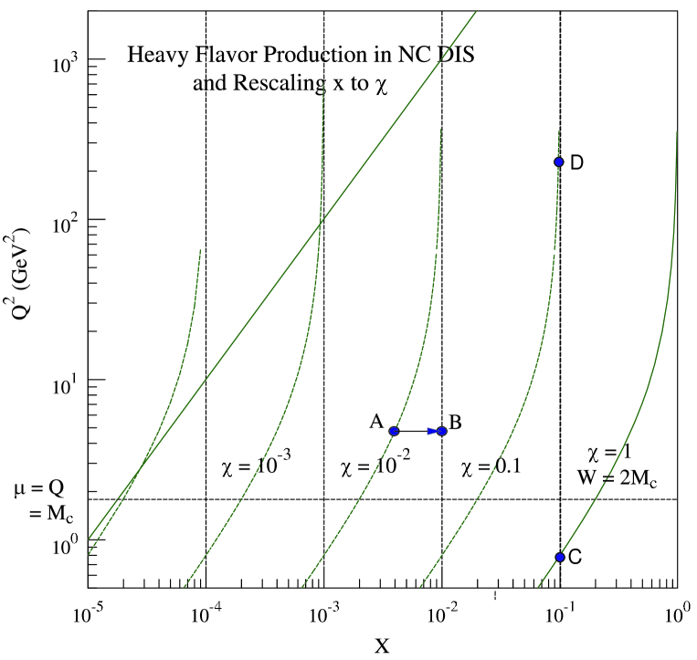
Figure 1: Kinematics of rescaling due to $M_{c}$ in the $(x,Q)$ plane for NC DIS. The curves are constant $\chi$ ($\chi_{c}$) lines. They asymptotically approach the corresponding Bjorken $x$ values (vertical lines). The solid diagonal straight line marks the kinematic reach of HERA.

In this plot, we show constant $x$ and constant $\chi_{c}$ lines. The threshold for producing charm corresponds to the line $W=2M_{c}$ (lower right corner), which coincides with $\chi_{c}=1$. Far above threshold, $\chi_{c}\simeq x$. Close to the threshold, $\chi_{c}$ can be substantially larger than $x$. For fixed (and sufficiently large) $x$, as $Q$ increases (along a vertical line upward in the plot, such as $x=0.1$), the threshold is crossed at $Q^{2}=4M_{c}^{2}\,x/(1-x)$ (point C on the plot), beyond which $\chi_{c}$ decreases, approaching $x$ asymptotically (point D on the plot). For fixed $Q$, as $x$ decreases from $1$ (along a horizontal line to the left), the threshold is crossed at $x=\left(1+{4M_{c}^{2}}/{\,Q^{2}}\right)^{-1}$, below which $\chi_{c}$ is shifted relative to $x$ according to Eq. (5) or (6).

Rescaling shifts the momentum variable in the parton distribution function $f^{a}(\xi,\mu)$ in Eq. (2) to a higher value than in the zero-mass case. For instance, at LO, the structure functions at a given point A are proportional to $f(x,Q)$ in the ZM formalism; but, with ACOT$\chi$ rescaling, this becomes $f(\chi_{c},Q)$. The shift $x\rightarrow\chi_{c}$ is equivalent to moving point A to point B in Fig. 1.

In the region where $\left(\Sigma_{f}\,M_{f}\right)^{2}/Q^{2}$ is not too small, especially when $f(\xi,\mu)$ is a steep function of $\xi$, this rescaling can substantially change the numerical result of the calculation.  It is straightforward to show that, when one approaches a given threshold ($M_{N}+\Sigma_{f}~{}M_{f}$) from above, the corresponding rescaling variable $\chi\rightarrow 1$. Since generally $f^{a}(\xi,\mu)\longrightarrow 0$ as $\xi\rightarrow 1$, rescaling ensures a smoothly vanishing threshold behavior for the contribution of the heavy quark production term to all structure functions. This results in a universal, and intuitively physical, realization of the threshold kinematic constraint for all heavy flavor production processes.

2.5 Hard Scattering Amplitudes and the SACOT Scheme

The last quantity in the general formula Eq. (2) that we need to discuss is the hard scattering amplitude $\widehat{\omega}_{a}^{\lambda}\left(x,\frac{Q}{\mu},\frac{M_{i}}{\mu},\alpha_{s}(\mu)\right)$. These amplitudes are perturbatively calculable. To facilitate the discussion, consider the special case of charm production in a neutral current process. At LO and NLO, the Feynman diagrams that contain at least one heavy quark ($c$ or $\bar{c}$) in the final state are depicted in Fig. 2 for both the 3-flavor (lower) and 4-flavor (upper) schemes.

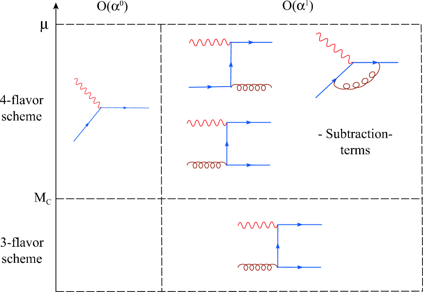
Figure 2: Partonic processes included in the theoretical $n_{f}$-flavor scheme calculations ($n_{f}=3,4$) at order $\alpha_{s}^{0}$ and $\alpha_{s}^{1}$. Generalization to higher orders is straightforward.

For $\mu<M_{c}$, the 3-flavor scheme applies. In this scheme, there is no charm parton in the initial state. The only diagram contributing to charm production at order $\alpha_{s}$ is the gluon fusion diagram. If $M_{c}$ is kept as nonzero, the hard scattering amplitude is finite; and the calculation is relatively straightforward. The hard scattering amplitude depends only on ($x,Q/M_{c}$), not on the factorization scale $\mu$.

For $\mu>M_{c}$, the 4-flavor scheme applies. The LO subprocess $\gamma/Z+c\rightarrow c$, with a charm parton in the initial state, is of order $\alpha_{s}^{0}$. It represents the resummed result of collinear singularities of the form $\alpha_{s}^{n}\ln^{n}(\mu/M_{c})$, $n=1,2,...$, from Feynman diagrams of all orders in $n$. Since the $\alpha_{s}\ln(\mu/M_{c})$ terms due to the NLO diagrams shown in Fig. 2 are already included in the resummation, they must be subtracted to avoid double-counting. These are denoted by the “subtraction terms” in Fig. 2. The subtraction term associated with the gluon-initiated diagram is of the form $\alpha_{s}\ln(\mu/M_{c})\omega^{0}(M_{c})\int_{\chi}^{1}(d\xi/\xi)\,g(\xi,\mu)P_{gq}(\chi/\xi)$ where $\omega^{0}(M_{c})$ is the LO hard scattering amplitude and $P_{gq}$ is the $g\rightarrow q$ splitting function of QCD evolution at order $\alpha_{s}$. The specific choices adopted for $\chi$, $\mu$, and the $M_{c}$ dependence of $\omega^{0}(M_{c})$ together precisely define the chosen factorization scheme. To be consistent, the same prescription must be used in evaluating the LO term, which takes the form $c(\chi,\mu)\,\omega^{0}(M_{c})$, where$c(\chi,\mu)$ is the charm parton distribution (cf. Eq. (13) in Appendix A).

The relation between the choice of $\chi$ (in the form of the rescaling variable $\chi_{c}$) and the proper treatment of kinematics was discussed in the previous subsection (Cf. also Appendix A). The freedom associated with the choice of the $M_{c}$ dependence of the hard scattering amplitudes was discussed in Refs. [8, 13]. The simplest choice that retains full accuracy can be stated succinctly as: keep the heavy quark mass dependence in the Wilson coefficients for partonic subprocesses with only light initial state partons ($g,u,d,s$); but use the zero-mass Wilson coefficients for subprocesses that have an initial state heavy quark ($c,b$). This is known as the SACOT scheme. For the 4-flavor scheme to order $\alpha_{s}$ (NLO), this calculational scheme entails: (a) keep the full $M_{c}$ dependence of the gluon fusion subprocess; (b) for NC scattering ($\gamma/Z$ exchanges), set all quark masses to zero in the quark-initiated subprocesses; and (c) for CC scattering ($W_{\pm}$ exchange), set the initial-state quark masses to zero, but keep the final-state quark masses on shell (Cf. [7, 13]).

2.6 Choice of Factorization Scale

The final choice that has to be made is that of factorization scale $\mu$, which connects the (soft) parton distributions and the hard scattering amplitude. Provided the matching between the LO and the subtraction terms are correctly implemented as described above (Sec. 2.5), the difference due to different choices of $\mu$ is formally of one order higher than that of the perturbative calculation—as long as $\mu$ is of the same order of magnitude as the physical hard scattering scale, say $Q$.  However, in the threshold region, the scale dependence can be quite sensitive to the treatment of kinematics because of heavy quark mass effects.  On the other hand, it was shown in Ref. [12] that, once the kinematics are handled correctly according to the ACOT$\chi$ prescription (Secs. 2.2–2.4), the $\mu$ dependence of the overall calculation becomes very mild.

In the conventional ZM formalism, the natural choice of the hard scale (the typical virtuality) for the DIS process is $Q$. Hence $\mu=Q$ is almost universally used in all practical calculations. In the GM formalism, we should re-examine the possible choices.

The total inclusive structure function $F_{i}^{tot}$ is infrared safe. Consider the simple case of just one effective heavy flavor, charm (i.e. below the bottom and top production thresholds),

$$F_{i}^{tot}=F_{i}^{light}+F_{i}^{c}\ ,$$ (7)

for any given flavor-number scheme (i.e. 3-flavor, 4-flavor, … etc.). If we use the same factorization scale $\mu$ for both terms, then the sum is insensitive to the value of $\mu$—the logarithmic $\mu$-dependence of the individual terms cancel each other.  Since the right-hand side of Eq. (7) is dominated by the light-flavor term $F_{i}^{light}$, and the natural choice of scale for this term is $\mu=Q$, it is reasonable to use this choice for both terms.  This turns out to be a good choice in practice as well, since the resulting $F_{i}^{tot}$ is then continuous across the boundary separating the 3-flavor region ($\mu<M_{c}$) from the 4-flavor region ($\mu>M_{c}$)—the line $Q=M_{c}$ in Fig. 1.

Experimentally, the semi-inclusive DIS structure functions for producing a charm particle in the final state $F_{i}^{c}$ is often presented. Unfortunately, theoretically, $F_{i}^{c}(x,Q,M_{c})$ is not infrared safe beyond NLO. One may nonetheless perform comparison of NLO theory with experiment with the understanding that the results are intrinsically less reliable, and they can be sensitive to the choice of parameters. The analytic expressions for $F_{i}^{c}$ in PQCD suggest that the typical virtuality for this process is $\sqrt{Q^{2}+M_{c}^{2}}$ instead of $Q$. For the factorization scale in this case, the choice $\mu=\sqrt{Q^{2}+M_{c}^{2}}$ appears to be natural. This choice has the added advantage that $\mu>M_{c}$ for all physical values of $Q$; hence, in practice, with this choice, one stays always in the 4-flavor regime, avoiding the need to make a transition from 3- to 4-flavor calculations when $Q$ crosses the value $M_{c}$, cf. Fig. 1.

3 Differences between ZM and GM calculations

The GM version of the $n$-flavor scheme calculation reduces to the conventional ZM one when the hard scale $Q$ is much larger than the quark mass $M_{n}$. Thus differences between the two schemes are only expected to be noticeable in the $Q\sim M_{n}$ region. Similarly, the differences between the GM and ZM versions of the VFNS should occur mostly around the charm, bottom and top threshold regions of the $(x,Q)$ plane.

In general, among the various mass effects described in the previous section, the most significant one numerically is that due to rescaling, $f(x,\mu)\rightarrow f(\chi,\mu)$. The size of this effect depends on: (i) the size of the shift $x\rightarrow\chi$; and (ii) the rate of change of $f(x,\mu)$ at the relevant value of $x$.  As can be seen from Fig. 1, the size of the shift $x\rightarrow\chi$ is largest when $Q\sim M_{n}$. According to (ii) above, however, this effect will be significant only when $f(x,\mu)$ is large and rapidly varying in $x$. As we shall see below, this effect shows up most prominantly at small $x$.

In the left panel of Fig. 3, we show the fractional differences between the GM and ZM calculations for $F_{2}^{\gamma}(x,Q)$ over the $(x,Q)$ plane. The magnitude of the fractional difference (in percentage) is represented by the color coding shown along the right vertical axis, and by the dashed contour lines.  The light solid curves are constant $\chi$ lines, taking into account the $c$ and $b$ quark masses. The kinematic boundary (blue line) corresponds to the HERA energy reach. We see that the expectations of the previous paragraph are borne out.

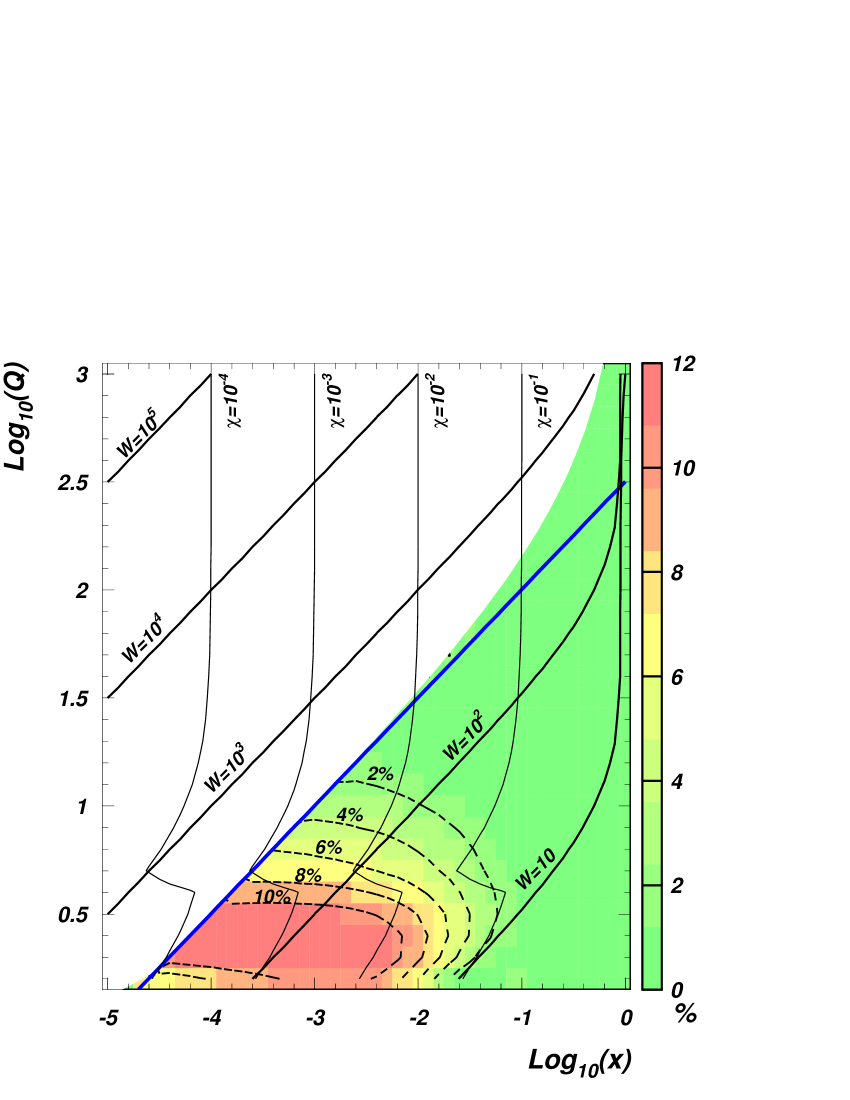
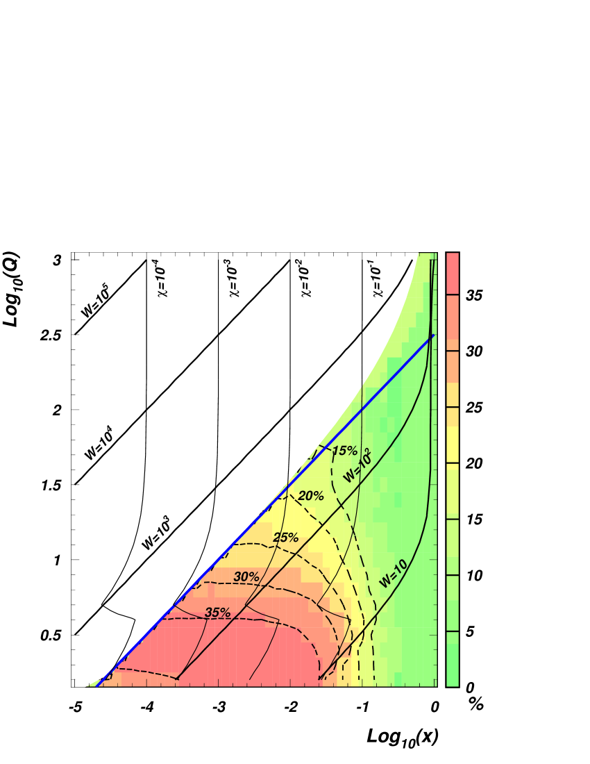
Figure 3: Fractional differences in percentages between the general-mass (GM) and zero-mass (ZM) calculations of $F_{2}^{\gamma}$ (left plot) and $F_{L}^{\gamma}$ (right plot), represented by color coding marked along the right-side vertical axis and by the dashed contour curves.

Mass effects can be more readily seen for physical quantities that vanish in the ZM limit. The most obvious example is the longitudinal structure function in DIS, $F_{L}(x,Q)$, which vanishes at LO in the ZM formalism. It is therefore useful to examine the importance of mass effects in $F_{L}$ quantitatively. In the right panel of Fig. 3, we show the fractional differences between the GM and ZM calculations for $F_{L}^{\gamma}(x,Q)$ over the ($x,Q$) plane.  Compared to the $F_{2}$ case, we see that, in addition to the effects of rescaling, the mass effects in the hard scattering is quite prominent. (Notice the different vertical scales of the two plots.) We see that the differences are more noticeable and spread wider in the charm and bottom threshold region than for the $F_{2}$ case, due to the additional mass effects in the hard scattering amplitude.

The differences between the GM and ZM calculations demonstrated here will have an impact on the global QCD analysis of PDFs, since the precision DIS data sets from both fixed-target and HERA cover the kinematic region highlighted in the above plots. Going from a ZM to a GM global analysis, the PDFs will undergo some re-alignment among themselves. And, for reasons described above, noticeable differences in the predictions for $F_{L}$ are expected.

4 New Global Analysis

We now apply the improved implementation of the GM formalism to the global QCD analysis of the full HERA I DIS cross section data sets (cf. next subsection), along with fixed-target DIS, Drell-Yan (DY) data sets and Tevatron Run I inclusive jet production data sets that were used in previous CTEQ global PDF studies, in order to obtain the most precisely determined parton distributions possible.

4.1 Input to the Analysis

Previous CTEQ global analyses of PDFs used structure function data for all available DIS experiments. By now, both H1 and ZEUS experiments have published detailed cross section data from the HERA I runs (1994 - 2000) for both NC and CC processes. We are able to use these cross section data directly in the global analysis, so that the new analysis is free of the model-dependent assumptions that usually go into the extraction of structure functions. This is important since, in addition to the dominant $F_{2}^{\gamma,\gamma Z}$, we can also gain model-independent information on the longitudinal and parity violating structure functions $F_{L}^{\gamma,\gamma Z}$ and $F_{3}^{\gamma Z}$ from this more comprehensive study. For this new effort to yield more accurate PDFs, and to produce more reliable predictions on the various structure functions mentioned above, it is crucial to use the available correlated systematic errors in the global analysis, as we shall discuss below.

The HERA I cross section data sets that are included in this analysis consist of the total inclusive NC and CC DIS processes, as well as the semi-inclusive DIS processes with tagged final state charm and bottom mesons. They are listed in Table I.

H1 94-97 CC $\sigma_{tot}$ [14] 96-97 NC $\sigma_{tot}$ [15] NC $F_{2}^{c}$ [16] 98-99 $e^{-}p$ NC $\sigma_{tot}$ [17] CC $\sigma_{tot}$ [17] 99-00 $e^{+}p$ NC $\sigma_{tot}$ [18] CC $\sigma_{tot}$ [18] NC $\sigma_{c}$ [19, 20] NC $\sigma_{b}$ [19, 20] $e^{-}p$ NC $\sigma_{tot}$ [18] ZEUS 94-97 $e^{+}p$ CC $\sigma_{tot}$ [21] 96-97 NC $\sigma_{tot}$ [22] NC $F_{2}^{c}$ [23] 98-99 $e^{-}p$ NC $\sigma_{tot}$ [24] CC $\sigma_{tot}$ [25] NC $F_{2}^{c}$ [26] 99-00 $e^{+}p$ NC $\sigma_{tot}$ [27] CC $\sigma_{tot}$ [28]

Table 1: HERA I table sets used in the global analysis.

These data are supplemented by fixed-target and hadron collider data sets used in the previous CTEQ global fits: BCDMS, NMC, CCFR, E605 (DY), E866 proton-deuteron DY ratio, CDF $W$-lepton asymmetry, and CDF/D0 inclusive jet production. Details and references to these can be found in Ref. [2]. We adopt the same $Q$- and $W$- cuts on experimental data as in Ref. [2]; and the stability of our results with respect to varying these cuts has been studied and reported in Ref. [29].

4.2 Parametrization of non-perturbative initial PDFs

The parametrization of the non-perturbative parton distribution functions is an important aspect of global QCD analysis since the robustness and reliability of the resulting PDFs depends on a delicate balance between allowing enough flexibility in the functional forms adopted to represent the unknown physics on the one hand, and avoiding over-parametrization that exceeds the constraining power of the available experimental input on the other.

For this round of analysis, we have carefully re-examined this issue, and tried a variety of functional forms, including exploring the number of degrees of freedom associated with each parton flavor that current experimental data can constrain. (A more detailed discussion is given in Sec. 5 on quantifying uncertainties). Results that are common to many reasonable choices of parametrization are considered trustworthy; the most representative among the stable fits are then chosen as the new standards. This effort results in some minor streamlining of the parametrization used in previous CTEQ analyses [2]. Details are given in Appendix B.

As with the previous analysis, we choose the input scale of $\mu_{0}=1.3$ GeV (which is also the charm quark mass, $M_{c}$, used in our calculations). We assume the strange and anti-strange quarks are equal to each other ($s=\bar{s}$), and are proportional to the non-strange sea combination $(\bar{u}+\bar{d})$ at $\mu_{0}$. We find that, within the current global analysis setup, the proportionality constant $\kappa$ (defined as $(s+\bar{s})/(\bar{u}+\bar{d})$) is only weakly constrained. For the purpose of the current analysis, we use the common value of $\kappa=0.5$ (at $\mu_{0}=1.3$ GeV) that is well within the allowed range. Finally, as in all existing global analyses, we assume the $c$ and $b$ distributions to be zero at the scale corresponding to their masses, and are generated by QCD evolution above that.

4.3 New Global Fits

The new global fit with the improved theoretical calculation and more extensive DIS data sets results in even better agreement between theory and experiment than the previous fits of CTEQ6M/CTEQ6.1M [2], CTEQ6HQ [30], and CTEQ6AB [31]. This is an important confirmation of the standard model (SM) in general, and the general mass PQCD formalism described in Sec. 2 in particular.

We choose a new central fit, designated as CTEQ6.5M, and 40 sets of eigenvector PDFs that form an orthonormal basis characterizing estimated uncertainties in the parton parameter space according to the Hessian method described in [32, 2]. We shall describe the characteristics of the central fit in this section, and the full eigenvector sets in a later section on uncertainties (Sec. 5).

The experimental data that have the most influence on the determination of the PDFs are, as is well known, the precision DIS total inclusive measurements, along with the DY experiments (sea quarks), $W$ lepton asymmetry measurements (flavor differentiation), and collider inclusive jet production measurements (gluon). New to the current global analysis (in addition to the replacement of NC structure functions by the more complete cross section data) are the HERA CC total inclusive and NC tagged heavy flavor inclusive structure functions and cross sections. These new data sets are fit quite well in the new round of global analyses, demonstrating the consistency of the underlying PQCD framework. However, due to the limited statistics available for these processes, they do not provide any readily identifiable constraints within the confines of the general global analysis procedure. More dedicated studies, with targeted techniques, may be needed to uncover potential physical implications of these data and their HERA II successors. We shall not pursue these in this paper.

As examples of the new fits to the HERA I cross section data, we show two plots comparing the H1 and ZEUS 1999-2000 $e^{+}p$ NC reduced cross section data sets with the CTEQ6.5M fit.

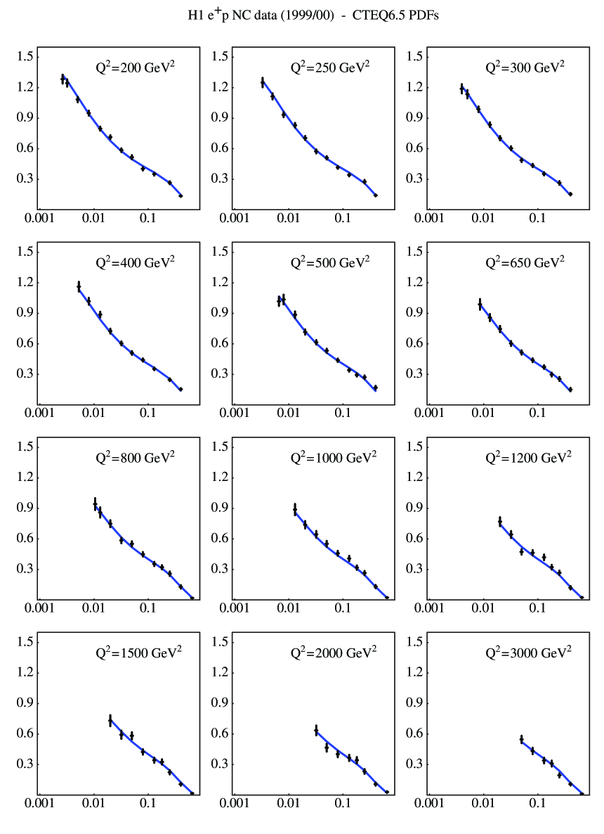
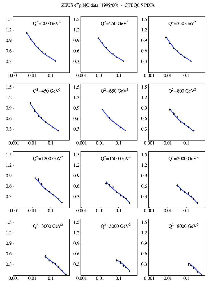
Figure 4: Comparison of the H1 (left) and ZEUS (right) 1999-2000 $e^{+}p$ NC reduced cross section data sets with the CTEQ6.5M fit.

The $\chi^{2}/$Npts (number of data points) for the two data sets are 169/147 and 94/90 respectively. The H1 data set has 6 sources of correlated systematic errors $\{r_{i},i=1,6\}$. The optimal shifts of these errors for the CTEQ6.5M fit are $\{r_{i}\}=\{0.378$, $-0.173$, $0.413$, $0.329$, $0.544$, $-0.515\}$—all within one $\sigma$, and $\sum_{i=1}^{6}r_{i}^{2}=1.012$. (The definition of the $r_{i}$ parameters, as used in our treatment of correlated errors, can be found in Appendix B of [2].) The ZEUS data set has 8 correlated systematic errors. The corresponding shifts are $\{r_{i}\}=\{0.096$, $-0.110$, $-0.048$, $0.385$, $-0.068$, $-0.651$, $-0.376$, $-1.334\}$—with only the last one being above 1, and $\sum_{i=1}^{8}r_{i}^{2}=2.522$. Both are quite reasonable. This pattern is typical for other HERA data sets. Details are available upon request to the authors.

4.4 New Parton Distributions

Since both the updates in theory and in experimental input in this global analysis represent incremental improvements over the previous CTEQ effort, rather than major modifications, we do not expect drastic shifts in the resulting PDFs. In the following discussions, we will focus on the few notable differences and their physical implications.

To highlight the changes in the PDFs, we present the ratio of the new CTEQ6.5M distributions and the corresponding CTEQ6.1M ones, compared to the previously estimated uncertainty bands of the latter. Figure 5 shows the d-quark, u-quark and gluon distributions at $Q=2$ GeV. The CTEQ6.5M/CTEQ6.1M ratios are represented by the solid curves.

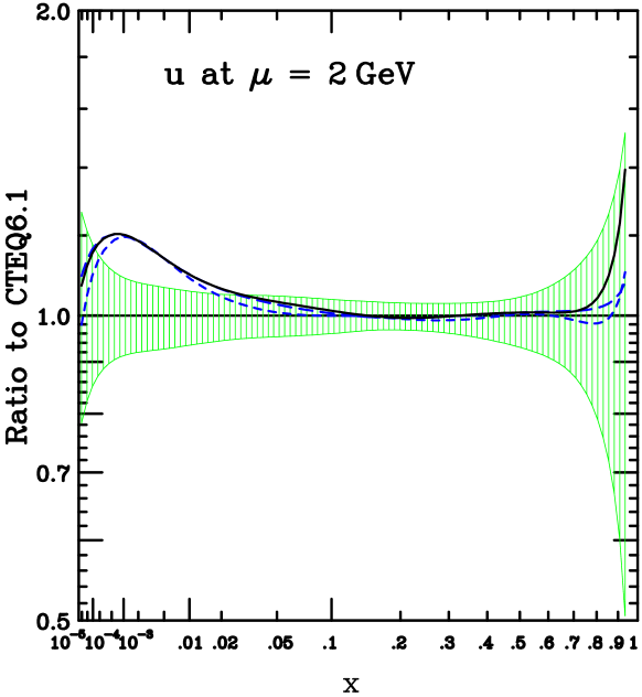
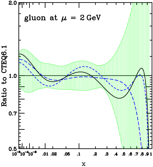
Figure 5: CTEQ6.5M $u,d$ and $g$ distributions (solid curves) at scale $\mu=2$ GeV normalized to the corresponding ones from CTEQ6.1M. The shaded areas represent the estimated uncertainty band from the CTEQ6.1 analysis. The dashed curves represent alternative, equally viable, candidates for this round of global analysis with slightly different parametrization forms than CTEQ6.5M.

To illustrate the universal behavior of the new fits, we also include two dashed curves in each plot, representing equivalent good fits with alternative parametrizations mentioned earlier (second paragraph of Sec. 4.2). We do not show separate results on the sea and the valence distributions, since the $u$- and $d$-quark distributions are dominated by the former at small $x$, and the latter at large $x$—both visible in the existing plots.

We see from Fig. 5 that the new PDFs are indeed generally within the previously estimated uncertainty bands, demonstrating consistency with previous analyses. There is, however, a notable departure of the new quark distributions from the old ones in the region $x\sim 10^{-3}$. At the peaks of the ratio curves, the new distributions are up to 20% larger than CTEQ6.1M, and a factor of two outside the previously estimated error bands. This feature is shared by all choices of alternative parametrizations (and by all 40 sets of eigenvector PDFs to be discussed in the next section).

It is not surprising to see a shift in the extracted quark PDFs in the small-$x$ and low-$Q$ region, since this is where the theoretical treatment of quark mass effect matters (cf. Sec. 3, particularly the left plot of Fig. 3). To see that this shift is indeed caused by mass effects in the new calculation, we compare $F_{2}(x,Q^{2}=4$ GeV${}^{2})$ calculated using CTEQ6.5M PDFs with the general-mass and the zero-mass Wilson coefficients, both normalized to the CTEQ6.1M result (which was obtained in the ZM formalism) in Fig. 6.

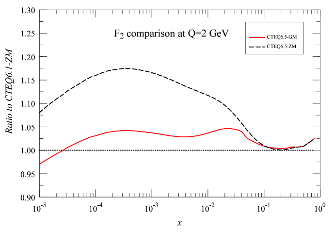
Figure 6: Comparison of theoretical calculations of $F_{2}$ using CTEQ6.1M in the ZM formalism (horizontal line of 1.00), CTEQ6.5M in the GM formalism (solid curve), and CTEQ6.5M in the ZM formalism (dashed curve).

The difference between the two CTEQ6.5M calculations is broadly in the small-$x$ region, and it is of similar order of magnitude to that seen in Fig. 5. Since the GM calculation (solid curve) yields lower values than the ZM calculation (dashed curve), the new CTEQ6.5M quark PDFs are pushed up in the new global analysis (cf. Fig. 5) in order to fit the same DIS data. The deviation of the GM CTEQ6.5M prediction is not far from the ZM CTEQ6.1M result (horizontal reference line, $1.00$) in Fig. 6 since both are obtained by fits to the data. However, they are not identical because there are several differences between the old and new global fits—DIS cross sections vs. structure functions as input, parametrization, etc.—in addition to the treatment of heavy quark mass effects.

The heavy quark mass effects diminish with increasing $Q^{2}$. However, their effect on the analysis of experiments at low $Q^{2}$ produces a change in the PDFs even at larger $Q^{2}$.

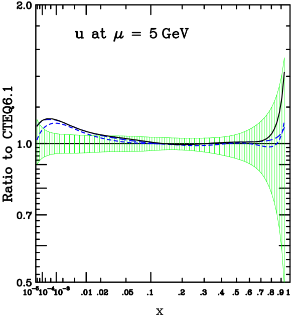
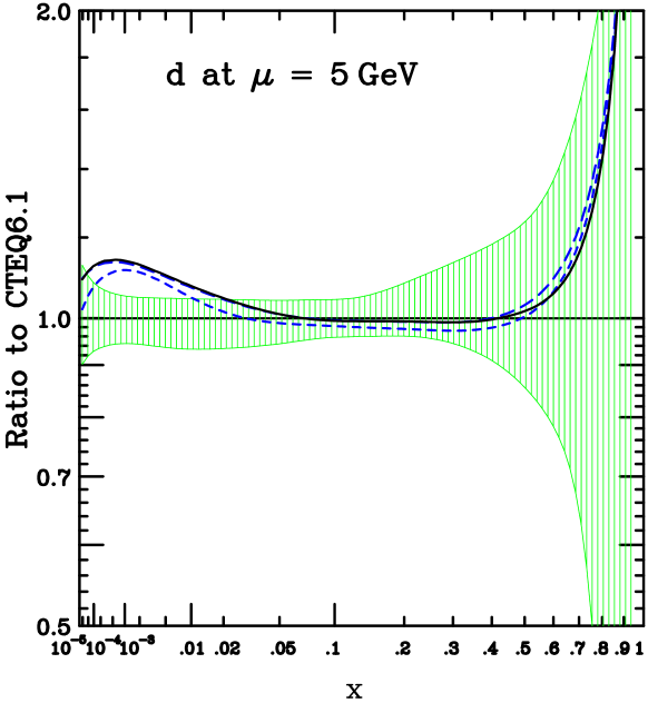
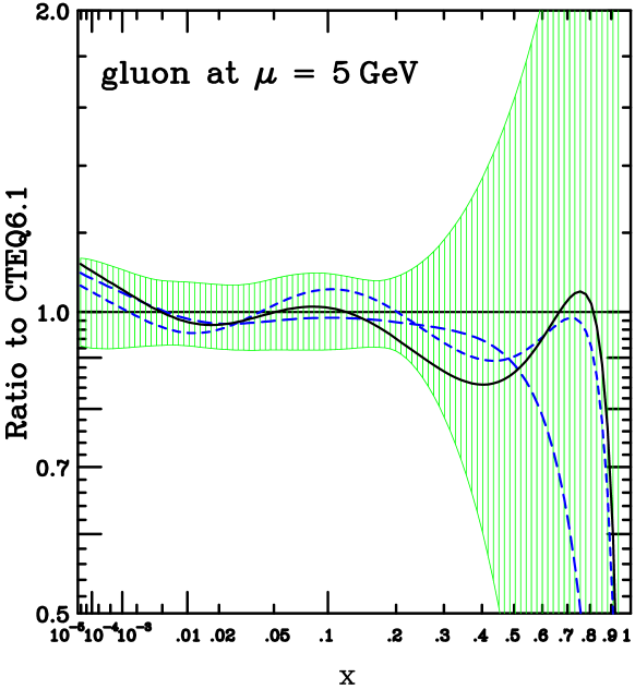
Figure 7: Same as Fig. 5, except that the PDFs are at the scale $\mu=5$ GeV.

Figure 7 shows the same comparisons at the scale $Q^{2}=25\,\mathrm{GeV}^{2}$. We see that the difference between CTEQ6.5M and CTEQ6.1M remains significant at this scale. Even at $Q^{2}\sim 10^{4}\,\mathrm{GeV}^{2}$, the CTEQ6.5 quark PDFs are higher than CTEQ6.1 by $\sim 5-6\%$ for $x\sim 10^{-3}$—approximately the CTEQ6.1 uncertainty at these $(x,Q)$ values. This can result in significant increases in physical predictions on hadron collider cross sections that are sensitive to PDFs in this $x$ range, e.g. for $W/Z$ production at the LHC, the increase is $\sim 8\%$, cf. Sec. 6.

4.5 Mass effects, Low-$Q^{2}$ HERA data, and Correlated systematic errors

The noticeable changes in the quark distributions at low $x$ and $Q$ also suggest a closer examination of the comparison of the new theoretical predictions with the precision DIS data in this region, particularly because the longitudinal structure function is expected to play a substantive role in the understanding of the low $x$ and $Q$ HERA cross section data.

Among the high precision HERA I data sets, the 1996-97 $e^{+}p$ NC reduced cross section measurements include data in the low $x$ and $Q$ region. We examine these data sets (from H1 [15] and ZEUS [22] ) in a little more detail. The CTEQ6.5 fit to the H1 data set has $\chi^{2}/\mathrm{Npts}=107\,/\,115$; the shifts of the 5 correlated systematic errors are $\{r_{i}\}=\{0.218$, $1.361$, $-0.472$, $0.374$, $1.581\}$ with $\sum r_{i}^{2}=4.763$. The corresponding numbers for the ZEUS data set are $\chi^{2}/\mathrm{Npts}=279\,/\,227$; the shifts of the 10 correlated systematic errors are $\{r_{i}\}=\{-1.575$, $-0.573$, $-1.407$, $-0.263$, $-0.025$, $-1.203$, $1.278$, $0.425$, $-0.258$, $0.238\}$, with $\sum r_{i}^{2}=8.244$. Aside from the somewhat high overall $\chi^{2}$ for the ZEUS data set (which was also seen in the previous round of CTEQ6.1 analysis using the corresponding $F_{2}$ data set), these numbers indicate reasonable fits.

In Fig. 8, we show the data from each experiment from the four lowest $Q$-bins that pass our $Q>2\,\mathrm{GeV}$ cut, normalized to the CTEQ6.5M fit.

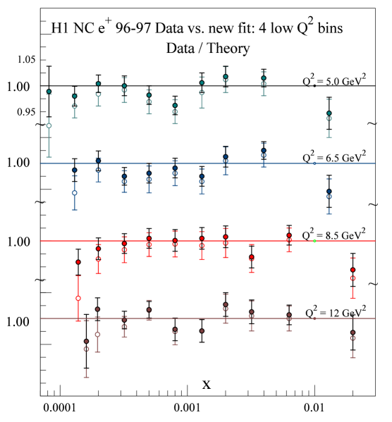
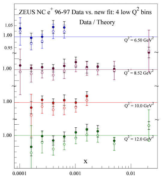
Figure 8: Four low $Q$ bins of the H1 and ZEUS 1996-97 NC cross section data sets compared to the CTEQ6.5M fit. Open circles: the ratio data/theory; solid dots: the same data points shifted by correlated systematic errors. (See text.)

The comparison with H1 data (left plot) shows a pattern of “turnover” of experimental data points (open circles) at low $x$ with respect to the theory for all four $Q^{2}$ bins. (For given $E$ and $Q$, low $x$ corresponds to high $y$.) However, this discrepancy disappears when correlated systematic errors are included in the analysis, as seen from the fact that the solid dots (representing data corrected by systematic errors) fit rather well the theory predictions (the horizontal lines corresponding to $1.00$ for the ratio). The values for the overall $\chi^{2}$ of this fit as well as the systematic shifts given in the previous paragraph support this observation.

The comparison of the ZEUS data to the CTEQ6.5M fit (right plot) does not show the same systematic low-$x$ turnover. Instead, data (open circles) in the three higher $Q$ bins are generally below the theory prediction. Again, we see that the differences between the two go away when correlated systematic errors are included in the analysis (solid dots). We get acceptable fits in all bins with reasonable systematic shifts.

The low-$Q$ and high-$y$ HERA data has been the subject of special analyses by both H1 and ZEUS collaborations, mainly in the context of extracting the longitudinal structure function $F_{L}(x,Q)$. Results of QCD fits performed in this regard [15, 33], appear to be similar to those shown above. Detailed comparison, however, is not possible at present since details of the theoretical input to the HERA analyses (e.g. issues related to mass effects described in Sec. 2) has not been specified. As we have shown, heavy quark mass effects are important in this kinematic region.  It would be useful for all future analyses to include the mass effects.

The observed low-$x$ turnover of the H1 data has been considered a potential problem for global analyses by the MRST group [34, 35]. This difficulty does not seem to arise in our analysis. Two possible sources could be responsible for this difference: (i) although both analyses include quark mass effects, the implementations are not the same (cf. [10], compared to Sec. 2); (ii) our inclusion of correlated systematic errors in the analysis is responsible for bringing theory and experiment into agreement, as demonstrated in Fig. 8. A more detailed study of these issues is clearly called for.

5 Uncertainties on New Parton Distributions

Using the new theory implementation and experimental input, we have also performed a detailed study of the uncertainties of the PDFs, following the Hessian method of [36, 32, 37, 2].  This involves finding a set of eigenvector PDFs that characterize the uncertainties of the parton distributions around the “best fit” in the parton parameter space.

To ensure that this procedure will yield meaningful results, we first carry out a series of studies to match our fitting parametrizations with theoretical and experimental constraints: (i) first we make sure that the best fit is robust by checking that the quality of the global fit cannot be significantly improved by increasing the number of free parameters or changing the functional forms; (ii) next, we identify “flat directions” in the resulting parameter space (representing degrees of freedom that are not constrained by current experimental input) by diagonalizing the Hessian matrix and examining its variation along the eigenvector directions; (iii) using that information, we freeze an appropriate subset of parameters and re-diagonalize the Hessian matrix, which characterizes the quadratic dependence of $\chi^{2}$ on the fitting parameters in the neighborhood of the minimum. The number of eigenvectors that can reasonably be determined is around 20—the same as was used in the CTEQ6.1 analysis.

To arrive at a quantitative estimate of the range of uncertainties in the parton parameter space, we examine the global $\chi_{\mathrm{global}}^{2}$ that is used by the fitting program as a measure of the overall “goodness-of-fit”, as the parameters are varied in the neighborhood of the global minimum. In defining $\chi_{\mathrm{global}}^{2}$, we include weight factors for a few experiments that have only a small number of data points. The eigenvectors and the weights are arrived at by the iterative method of Ref. [36] so that an adequate fit to every data set is maintained as far out as possible along the eigenvector directions. This allows us to estimate a confidence range by the condition that, within this range, the fit to every data set is within its 90% confidence level.

In this way we generate the final eigenvector PDF sets so that they span the 90% confidence range for the contributing data sets. The procedure is similar to that formulated in Refs. [37, 32, 2] (which contains more details). There are 40 eigenvector sets, corresponding to displacements from the central fit in the “$+$” or “$-$” senses along each of the eigenvector directions. PDF uncertainty limits for a 90% confidence range for physical predictions can be calculated from these sets by computing the prediction for each of the 40 sets, and adding the approximately 20 upward (downward) deviations in quadrature to obtain the upper (lower) limit.

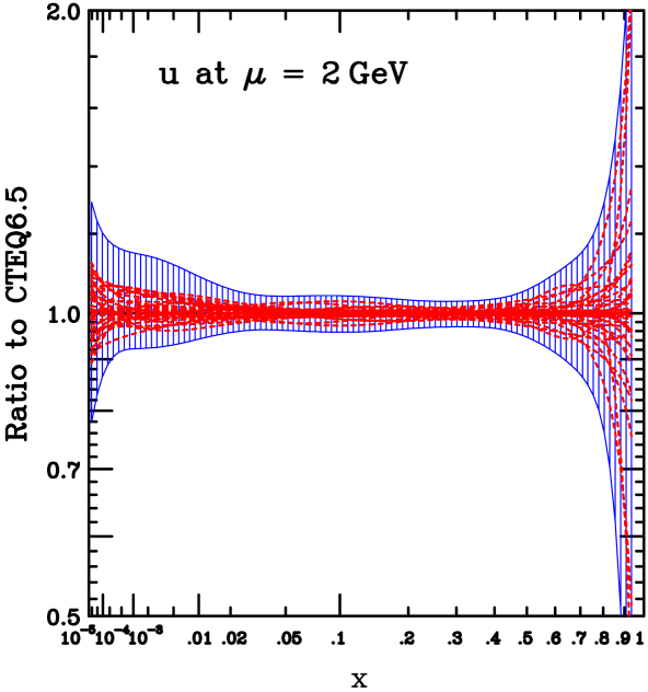
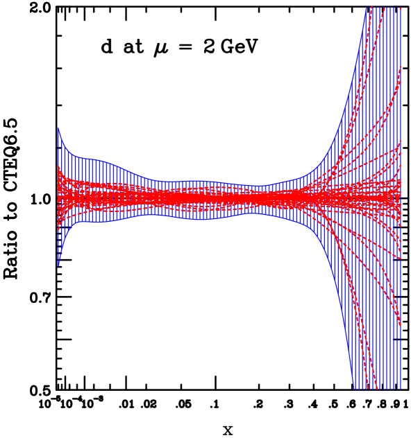
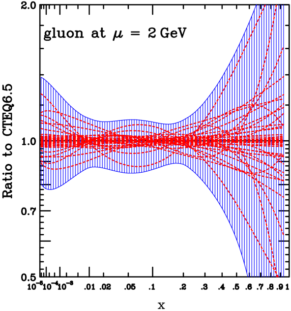
Figure 9: CTEQ6.5 PDF uncertainty bands and eigenvector PDF sets.

Figure 9 shows the uncertainty bands determined by this method for $u$, $d$, and $g$ PDFs at the scale $Q^{2}=4\,\mathrm{GeV}^{2}$. The lines represent each of the 40 sets of eigenvector PDFs normalized to the central fit. The upper (lower) edges of the shaded uncertainty region is obtained by adding in quadrature the contributions from eigenvector sets that lie above (below) the central fit at each particular $x$. We observe that, in some cases (such as for the gluon at large $x$), the uncertainty band is dominated by a single pair of eigenvector PDFs, corresponding to the two senses along a single eigenvector direction.

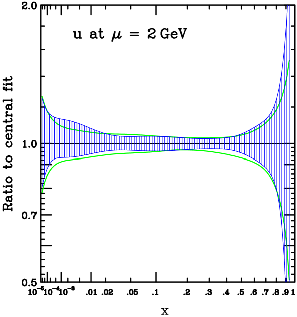
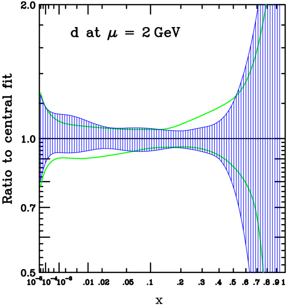
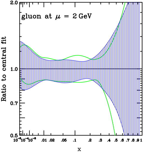
Figure 10: CTEQ6.5 PDF uncertainty bands compared to those of CTEQ6.1.

Figure 10 shows the same uncertainty bands as above, together with curves that show the fractional uncertainty range from CTEQ6.1 that was determined by a similar procedure. This shows that the two estimates of PDF uncertainties are broadly comparable with each other, with a slight tightening of the uncertainty ranges of $d$ quark and gluon distributions in certain $x$ regions. Of more interest is a comparison of estimated uncertainties of physical predictions. We shall discuss these in Sec. 6 below.

Because of the improved theoretical and experimental input to this new global analysis, as well as the much more thorough study of its parametrization dependence, we now have greater confidence in these uncertainty estimates than before. Wider applications of the new results to Standard Model and New Physics processes at hadron colliders will be pursued.

To compare some currently used PDFs to that of CTEQ6.5, Figure 11

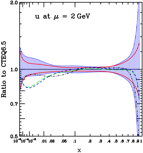
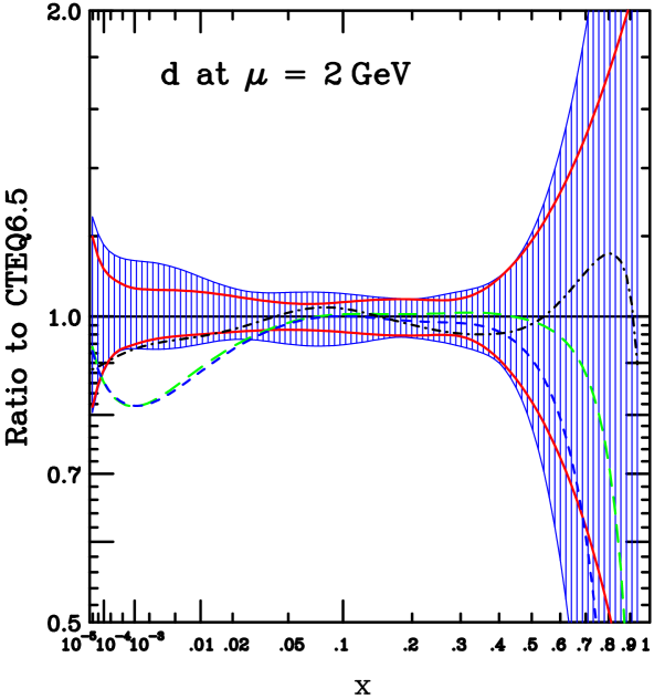
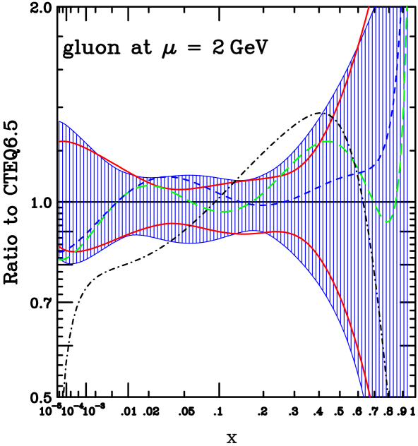
Figure 11: Same CTEQ6.5 PDF uncertainty bands compared to: (i) the CTEQ6.1M (green long-dash line), CTEQ6A118 (blue short-dash) and MRST04 (black dash-dotted) PDFs; and (ii) upper and lower edges (red solid lines) of similar uncertainty bands generated with reduced number of fitting parameters (see text).

shows CTEQ6.1M (dashed curves), CTEQ6A118 (central fit of the CTEQ6 “$\alpha_{s}$ series” [31]), and MRST04 [3] PDFs as ratios to CTEQ6.5M. We note that the previous CTEQ PDFs lie mainly within the new uncertainty bands—except at $x\sim 10^{-3}$ for the reasons discussed in the various subsections of Sec. 4. The MRST04 quark PDFs are closer to CTEQ6.5 in the $x\sim 10^{-3}$ region than CTEQ6.1M and CTEQ6AB, presumably because both CTEQ6.5 and MRST04 include mass effects (albeit using different prescriptions) while the other two are in the ZM formalism. The MRST04 gluon PDFs are within the CTEQ6.5 uncertainty band at large-$x$; but they are outside the band around $x=0.3$ and at small $x$.

As mentioned earlier, as a part of our investigation on the robustness of our results, we have performed uncertainty analysis using different number of variable parameters. (Other global analysis groups have always used fewer variables.) We found the resulting ranges of uncertainty stable if this number is greater than 16. To show how the results may be affected by too restrictive choices of parameters, Figure 11 also include two curves (red) that correspond to the edges of the uncertainty bands using only 11 free parameters. We see that these bands are considerably narrower than the stable results represented by the CTEQ6.5 bands. In other words, over-restricting the degrees of freedom in the input parametrization at $\mu_{0}$ can significantly overestimate how well the PDFs are measured.

6 Implications for Hadron Collider Physics

The new PDFs have significant implications for hadron collider phenomenology at the Tevatron and the LHC. We shall mention one example here: the benchmark $W$ production total cross section $\sigma_{W}$.

The higher quark distributions in CTEQ6.5 for $x\sim 10^{-3}$ lead to an increase in the predicted values for $\sigma_{W}$ over those based on CTEQ6.1: for Tevatron Run II, we get $\Delta\sigma_{W}/\sigma_{W}=3.5\%$; and for the LHC, $\Delta\sigma_{W}/\sigma_{W}=8\%$. The significant increase of the predicted $\sigma_{W}$ at the LHC reflects the fact that it is directly dependent on PDFs in the region $x\sim 10^{-3}$.

It is also interesting to compare the uncertainties of these predictions as estimated by the Hessian method. For the Tevatron, we find this uncertainty to be $\mathrm{+}3.1/\mathrm{-}3.0\%$ for CTEQ6.5, compared to $\mathrm{+}3.8/\mathrm{-}4.4\%$ estimated using CTEQ6.1. For the LHC, the uncertainty is $\mathrm{+}4.9/\mathrm{-}4.1\%$ for CTEQ6.5, compared to $\mathrm{+}5.2/\mathrm{-}5.9\%$ for CTEQ6.1. Thus there is a notable reduction in the uncertainty ranges. This is perhaps related to a better determination of the correlations between different parton flavors, in addition to the obvious connection to the uncertainties of the individual PDFs (which are rather comparable for CTEQ6.1 and CTEQ6.5) shown in Figure 10.

Detailed results on W/Z production, including differential distributions, and implications of these new PDFs on other SM and New Physics processes for hadron colliders will be explored in a separate study.

7 Summary and Outlook

We have updated both the theoretical and experimental input to the CTEQ global QCD analysis in this work. On the theory side, we have used a newly implemented systematic approach to PQCD, including heavy quark mass effects according to the general formalism of Collins [8]. Experimentally, we have used all available precision HERA I cross section data sets, along with well-established fixed target and hadron collider experimental data. Correlated systematic errors, whenever available, are fully incorporated in the analysis. In performing this analysis, we have extensively studied the effects due to changes of the functional form for the initial parton distributions, and to changes in the number of free parameters allowed in the fits, in order to arrive at stable and physically meaningful results.

One noticeable common feature of the new parton distributions, compared to the previous ones, is the change in the $u$ and $d$ quark distributions around $x\sim 10^{-3}$ at low $Q$. This results from the inclusion of mass effects in the theory, in conjunction with the improved (model independent) HERA cross section data, over the previous analysis (using $F_{2}$ data that inevitably involve assumption about $F_{L}$ for their extraction).

Within the general-mass PQCD framework, we find broad consistency between the extensive data sets incorporated in this analysis. This permits us to arrive at 90% confidence level estimates of the uncertainties of PDFs around the chosen central fit, CTEQ6.5M. These uncertainties are encapsulated in 40 sets of eigenvector PDFs that span the neighborhood of the central fit in the parton parameter space. We found the new uncertainty bands of the PDFs are slightly narrower than the previous ones, but are generally of the same order of magnitude.

While progress towards better-determined PDFs in a more precisely formulated PQCD framework has clearly been made, it is worthwhile to mention some of the limitations of current global analysis of PDFs that call for continued advances in both theory and experiment. First, due to rather weak existing experimental constraints of the strange quarks, we have assumed in this work that $(s+\bar{s})$ is of the same shape as $(\bar{u}+\bar{d})$ and fixed the proportionality constant $\kappa$ at the initial scale $Q_{0}$ during the fit. In principle, better constraints on $\kappa$, and on the possible difference between $s$ and $\bar{s}$, can come from recent neutrino scattering experiments by NuTeV [38] and Chorus [39]. However, many open questions pertaining to the consistency between existing experimental data sets (including those from the “old” experiments CDHSW and CCFR), nuclear target corrections, and other issues make the use of these data controversial at present. A dedicated study on the strangeness sector, designed to delineate the range of uncertainties of both $s(x)$ and $\bar{s}(x)$, will require a somewhat different tactic, focused on the most relevant degrees of freedom. In the same vein, we have assumed that all heavy quark partons ($c$ and $b$) are generated radiatively by QCD evolution (mainly gluon splitting) at the initial scale $Q_{0}$. This assumption is not well defined quantitatively, because it depends on the choice of $Q_{0}$. Furthermore the assumption itself may be questioned—does intrinsic charm exist in the proton? The charm and bottom degrees of freedom can be investigated phenomenologically within the general-mass PQCD framework described here, and is currently under investigation [40].

There has been considerable discussion in recent literature [41] about extending global QCD analysis to higher orders in $\alpha_{s}$. This interest is spurred, on the one hand, by the final availability of the NNLO evolution kernel [42], and on the other hand, by the calculation of NNLO Wilson coefficients for various hard scattering processes, such as Higgs production [43]. In the global analysis of PDFs, NNLO becomes important, and, by implication, necessary to include, when the theoretical corrections to NLO calculations are comparable to the errors on the corresponding input experimental data. For DIS and DY processes used in current global analysis, this happens only in the small-$x$ region [42]. However, near boundaries of the kinematic region, such as small $x$, the relatively large corrections are generally associated with higher powers of large logarithms in PQCD. These are symptoms of the breakdown of the fixed-order perturbation expansion and the need to resum these logarithms in order to achieve stable and reliable results. Thus, efforts to expand global QCD analysis to higher orders must go hand-in-hand with work to incorporate resummation effects (not only confined to small $x$) in the theoretical framework. The importance of much development work along both lines is evident.

The new CTEQ6.5 PDF sets, including the eigenvector sets discussed in Sec. 5, will be made available at the CTEQ web site (http://cteq.org/) and through the LHAPDF system (http://hepforge.cedar.ac.uk/lhapdf/). Because the GM formalism used in this analysis represents a better approximation to QCD, compared to the previously used ones, the new PDFs are expected to be closer to the true values than previous ones. In physical applications at energy scales much larger than $M_{c}$ and $M_{b}$, these PDFs can be convoluted with commonly available hard-scattering cross sections calculated in the ZM formalism to obtain reliable predictions, because quark mass effects in the Wilson coefficients will be negligible. However, for quantitative comparison of a theoretical calculation to precision DIS data, in the region where $M_{c}/Q$ and $M_{b}/Q$ are not very small, the GM formalism described in Sec. 2 must be applied to the hard scattering cross section together with CTEQ6.5 PDFs in order to obtain accurate results.

Acknowledgements

We thank John Collins, Stefan Kretzer, and Carl Schmidt for discussions about the general PQCD framework, particularly the implementation of the general mass scheme; and Joey Huston for discussions on various issues about global analysis, as well as on the presentation of our results.

This work was supported in part by the U.S. National Science Foundation under awards PHY-0354838 and PHY-0555545; and by National Science Council of Taiwan under grant 94(95)-2112-M-133-001.

Appendix A Rescaling

We give here an intuitive derivation of the rescaling prescription (ACOT$\chi$) in the context of NC charm production. The general idea is applicable to other heavy flavor production processes, as will become clear later. As mass effects are only relevant at energy scales comparable to the heavy quark mass (charm in our case), we will focus in this region where the physically dominant mechanism for charm production is the gluon fusion process $\gamma^{\ast}g\rightarrow c\bar{c}$. The graphical representation of this process is shown as the first term in Fig. 12.

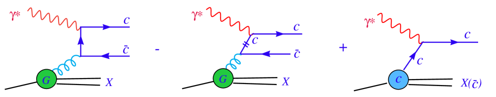
Figure 12: Contributions to charm production in NC DIS scattering and the physical origin of the rescaling variable in the PQCD approach.

The analytic expression for this contribution to the physical structure function is

$${\alpha_{s}(\mu)\int_{\chi_{c}}^{1}\frac{dz}{z}g(z,\mu)\omega_{\gamma^{\ast}g\rightarrow c\bar{c}}^{1}(\frac{\chi_{c}}{z},Q,M_{c})\rule{0.0pt}{12.91663pt}}$$ (8)

where ${\alpha_{s}\omega_{\gamma^{\ast}g\rightarrow c\bar{c}}^{1}}$ is the order ${\alpha_{s}}$ partonic cross section, ${g(z,\mu)}$ is the gluon distribution function. The lower limit of the convolution integral is determined by the boundary of the final state phase space integration; it is

$$\chi_{c}=x(1+4M_{c}^{2}/Q^{2})$$ (9)

with $x$ being the Bjorken $x$. We recognize that this is just the rescaling variable Eq. (6) of Sec. 2.4. For the gluon-fusion subprocess, it follows strictly from kinematics, once we include the mass of the heavy quarks into consideration.

The gluon fusion term by itself is not infrared safe at high energies.  In this limit, the infrared unsafe part comes from the collinear configuration in the final state phase space integration. The singular part of ${\omega_{\gamma^{\ast}g\rightarrow c\bar{c}}^{1}}$ is of the form

$${\omega_{\gamma^{\ast}g\rightarrow c\bar{c}}^{1}(z,,Q,M_{c})\rightarrow\ln(\frac{Q}{M_{c}})P_{g\rightarrow c}(z)\;\omega_{\gamma^{\ast}c\rightarrow c}^{0}}$$ (10)

where${\;\omega_{\gamma^{\ast}c\rightarrow c}^{0}}$ represents the order $\alpha_{s}^{0}$ process $\gamma^{\ast}c\rightarrow c$ (upper vertex of vector-boson coupling to quark); and ${P_{g\rightarrow c}(z)}$ is the $g\rightarrow c$ splitting function. This collinear singularity of the $\gamma^{\ast}g\rightarrow c\bar{c}$ contribution can be removed by a subtraction term of the form

$$-{\alpha_{s}(\mu)\ln(\frac{\mu}{M_{c}})\int_{\zeta}^{1}\frac{dz}{z}g(z,\mu)P_{g\rightarrow c}(\frac{\zeta}{z})\;\omega_{\gamma^{\ast}c\rightarrow c}^{0}}$$ (11)

with the introduction of the factorization scale $\mu$ (generally chosen to be of order $Q$). This term is represented by the second graph in Fig. 12, where the mark on the internal charm parton line signifies that its momentum $k$ is collinear to the gluon and $k^{2}\approx 0$. For the purpose of cancelling the collinear singularity of the gluon-fusion term at high energies (the Bjorken limit), the variable $\zeta$ in this expression can be any expression provided $\zeta\rightarrow x$ in that limit. In fact, conventionally, it is taken to be just $x$. The trouble with this choice is that in the other limit—near the threshold region where $W$ and $Q$ are of the order of $M_{c}$—the subtraction term knows nothing about the kinematics of $c\bar{c}$ pair production, hence bears no relation to the physical structure function. The combined result of Eqs. (8) and (11) is then completely artificial, hence unphysical, in this region. To remedy this problem, one only needs to realize the origin of the subtraction term, and make the obvious choice

$$\zeta=\chi_{c}=x(1+4M_{c}^{2}/Q^{2})$$ (12)

that is appropriate for the parent gluon-fusion contribution, Eq. (8). With this choice of the scaling variable $\zeta$, the subtraction term, Eq. (11) behaves correctly both in the high-energy and the low-energy regions.

To complete the derivation, we need to turn to the third diagram of Fig. 12, which represents the simple order-$\alpha_{s}^{0}$ $\gamma^{\ast}c\rightarrow c$ parton process in the 4-flavor scheme. From the perspective of the preceding discussion, this term arises from resumming the collinear and soft singularities to all orders in the perturbation expansion. The leading term in this expansion is given by Eq. (11) above (with a positive sign). The resummed result, as illustrated by the diagram, is just

$${c(\zeta,\mu)\;\omega_{\gamma^{\ast}c\rightarrow c}^{0}}$$ (13)

Here, the choice of the scaling variable $\zeta$ should be dictated by similar considerations as above: at high energies, $\zeta$ must reduce to the Bjorken $x$; and in the threshold region, the combined contribution from Eq. (13) and the subtraction term, Eq. (11), must be of higher order in $\alpha_{s}$. The naive (and common) choice $\zeta=$ $x$ satisfies the first criterion, but not the second. For the same reason discussed before, the choice $\zeta=\chi_{c}$, Eq. (12), satisfies both; hence it is the physically sensible one to use.

With the use of the rescaling variable $\zeta=\chi_{c}$ for the LO $\gamma^{\ast}c\rightarrow c$ term and the subtraction term, the sum of the three contributions in Fig. 12 reduces, by definition, to the gluon fusion contribution in the threshold region, as it should; and it approaches the conventional zero-mass PQCD form, LO ($\gamma^{\ast}c\rightarrow c$) + (NLO correction), in the high energy limit, as it should. From this perspective, one sees clearly the dual role of the subtraction term: in the threshold region, it overlaps substantially with the LO ($\gamma^{\ast}c\rightarrow c$) contribution to make the gluon fusion subprocess the primary production mechanism; and in the high energy limit, it overlaps with the singular part of the $\gamma^{\ast}g\rightarrow c\bar{c}$ contribution, and thus helps to render the combined order $\alpha_{s}$ terms infrared safe (and yield the true NLO correction to the perturbative expansion).

Appendix B Parametrization

The parametrization of the parton distributions at $\mu_{0}$ that was used to obtain the CTEQ5 and CTEQ6 parton distributions contained 5 shape parameters (apart from normalization) for each flavor. However, the global analysis data sets were not sufficiently constraining to determine all of these parameters, so a number of them were frozen at some particular values.

In the current effort to match the theoretical parametrization with experimental constraints, we achieve the same goal by adopting a simpler form with 4 shape parameters for the valence quarks $u_{v}(x)$, $d_{v}(x)$, and the gluon $g(x)$:

$$f(x)=a_{0}\,x^{a_{1}}\,(1-x)^{a_{2}}\,\mathrm{e}^{a_{3}x\,+\,a_{4}x^{2}}\;.$$ (14)

This can be seen as a plausible generalization of the conventional minimal form

$$f_{0}(x)=a_{0}\,x^{a_{1}}\,(1-x)^{a_{2}}\;,$$ (15)

which combines Regge behavior at $x\rightarrow 0$ and spectator counting behavior at $x\rightarrow 1$ in an economical way.

Both functions, (14) and (15), are conveniently positive definite. The following modified logarithmic derivatives of these functions are simple polynomials in $x$,

$$\phi_{0}(x)=-x\,(1-x)\,\frac{d\ln f_{0}}{dx}=-a_{1}+b_{1}x\;,$$ (16)

and

$$\phi(x)=-x\,(1-x)\,\frac{d\ln f}{dx}=-a_{1}+b_{1}x+b_{2}x^{2}+b_{3}x^{3}\;,$$ (17)

where the coefficients $\left\{b_{i}\right\}$ are simple linear combinations of the original ones $\left\{a_{i}\right\}$ in the exponent of Eq. (14). So the form Eq. (14) corresponds to generalizing the logarithmic derivative from a linear function $\phi_{0}(x)$ to a cubic polynomial $\phi(x)$, and follows in the spirit of using polynomials to approximate unknown functions that have no known singularities. The only practical question is whether this polynomial generalization contains enough flexibility to represent the physical PDFs that we are trying to determine. Our investigation indicates that this is the case, since significantly better fits cannot be achieved by introducing additional parameters or by changing the functional forms.

We continue to use the same parametrizations for $\bar{u}$, $\bar{d}$ that were used in CTEQ6. As mentioned in the text (Sec. 4.2), we continue to use the approximation $s(x)=\bar{s}(x)\propto\bar{u}(x)+\bar{d}(x)$. The full set of formulas for the initial PDFs at $\mu_{0}=1.3\,\mathrm{GeV}$ is

$$u_{v}(x),d_{v}(x),g(x) = A_{0}\,x^{A_{1}-1}\,(1-x)^{A_{2}}\,\mathrm{e}^{-A_{3}(1-x)^{2}\,+\,A_{4}x^{2}}$$ (18)

$$\bar{u}(x)+\bar{d}(x) = \textstyle{\frac{1}{2}}\,A_{0}\,x^{A_{1}-1}\,(1-x)^{A_{2}}\,\mathrm{e}^{A_{3}x}\,(1+x\mathrm{e}^{A_{4}})^{A_{5}}$$ (19)

$$\bar{d}(x)/\bar{u}(x) = \mathrm{e}^{A_{1}}\,x^{A_{2}-1}\,(1-x)^{A_{3}}\;+\;(1+A_{4}x)\,(1-x)^{A_{5}}$$ (20)

$$s(x)=\bar{s}(x) = \textstyle{\frac{1}{2}}\,\kappa\,(\bar{u}(x)+\bar{d}(x))$$ (21)

$$c(x)=\bar{c}(x)=b(x)=\bar{b}(x) = 0$$ (22)

(Notes regarding these formulas: the parameter $A_{1}$ is shifted from the $a_{1}$ above to make it correspond in definition to the standard Regge intercept; the parameters $a_{3}$ and $a_{4}$ are replaced by linear combinations $A_{3}$ and $A_{4}$ to reduce their correlation in the fitting by making them control behavior at large and small $x$; the parameter $A_{4}$ in $\bar{u}+\bar{d}$ is defined using an exponential form to ensure positivity of the PDFs.)

For concreteness, we give in Table II the coefficients that correspond to the central fit CTEQ6.5M. The value of $\kappa$ is $0.5$; and the strong coupling constant $\alpha_{s}(M_{Z})$ is $0.118$. We use $M_{c}=1.3\,\mathrm{GeV}$, $M_{b}=4.5\,\mathrm{GeV}$.

	$A_{0}$	$A_{1}$	$A_{2}$	$A_{3}$	$A_{4}$	$A_{5}$
$u_{v}$	$5.76388$	$0.64416$	$2.31531$	$0.74528$	$-2.14868$
$d_{v}$	$3.65786$	$0.62677$	$3.31531$	$0.87977$	$-2.37338$
$g$	$0.09974$	$0.22853$	$4.00000$	$-4.23974$	$8.64169$
$\bar{d}+\bar{u}$	$0.29563$	$-0.22165$	$12.09400$	$6.46763$	$4.51075$	$0.26278$
$\bar{d}/\bar{u}$		$11.49257$	$5.64186$	$17.00000$	$19.41872$	$9.45863$

References

- [1] T. Q. W. Group et al., “Tevatron-for-LHC report of the QCD working group,” arXiv:hep-ph/0610012.
- [2] J. Pumplin, D. R. Stump, J. Huston, H. L. Lai, P. Nadolsky and W. K. Tung, JHEP 0207, 012 (2002) [hep-ph/0201195]; D. Stump, J. Huston, J. Pumplin, W. K. Tung, H. L. Lai, S. Kuhlmann and J. F. Owens, JHEP 0310, 046 (2003) [hep-ph/0303013].
- [3] A. D. Martin, R. G. Roberts, W. J. Stirling and R. S. Thorne, Phys. Lett. B 604, 61 (2004) [hep-ph/0410230] and references therein.
- [4] W.K. Tung, Talk in Structure Function Work Group, DIS2006, Tsukuba, Japan, to be published in the proceedings.
- [5] J. C. Collins and W. K. Tung, Nucl. Phys. B 278, 934 (1986).
- [6] J. Collins, F. Wilczek, and A. Zee, Phys. Rev. D 18, 242 (1978).
- [7] M. A. G. Aivazis, J. C. Collins, F. I. Olness and W. K. Tung, Phys. Rev. D 50, 3102 (1994) [hep-ph/9312319].
- [8] J. C. Collins, Phys. Rev. D58, 094002 (1998) [hep-ph/9806259].
- [9] M. A. G. Aivazis, F. I. Olness and W. K. Tung, Phys. Rev. D 50, 3085 (1994) [hep-ph/9312318].
- [10] R. S. Thorne, Phys. Rev. D 73, 054019 (2006) [hep-ph/0601245], and references therein.
- [11] R. M. Barnett, Phys. Rev. Lett. 36, 1163 (1976); T. Gottschalk, Phys. Rev. D 23, 56 (1981).
- [12] W. K. Tung, S. Kretzer and C. Schmidt, J. Phys. G 28, 983 (2002) [hep-ph/0110247].
- [13] M. Kramer, F. I. Olness and D. E. Soper, Phys. Rev. D 62, 096007 (2000) [hep-ph/0003035].
- [14] C. Adloff et al. [H1 Collaboration], Eur. Phys. J. C 13, 609 (2000) [hep-ex/9908059].
- [15] C. Adloff et al. [H1 Collaboration], Eur. Phys. J. C 21, 33 (2001) [hep-ex/0012053].
- [16] C. Adloff et al. [H1 Collaboration], Phys. Lett. B 528, 199 (2002) [hep-ex/0108039].
- [17] C. Adloff et al. [H1 Collaboration], Eur. Phys. J. C 19, 269 (2001) [hep-ex/0012052].
- [18] C. Adloff et al. [H1 Collaboration], Eur. Phys. J. C 30, 1 (2003) [hep-ex/0304003].
- [19] A. Aktas et al. [H1 Collaboration], Eur. Phys. J. C 40, 349 (2005) [hep-ex/0411046].
- [20] A. Aktas et al. [H1 Collaboration], Eur. Phys. J. C 45, 23 (2006) [hep-ex/0507081].
- [21] J. Breitweg et al. [ZEUS Collaboration], Eur. Phys. J. C 12, 411 (2000) [Erratum-ibid. C 27, 305 (2003)] [hep-ex/9907010].
- [22] S. Chekanov et al. [ZEUS Collaboration], Eur. Phys. J. C 21, 443 (2001) [hep-ex/0105090].
- [23] J. Breitweg et al. [ZEUS Collaboration], Eur. Phys. J. C 12, 35 (2000) [hep-ex/9908012].
- [24] S. Chekanov et al. [ZEUS Collaboration], Eur. Phys. J. C 28, 175 (2003) [hep-ex/0208040].
- [25] S. Chekanov et al. [ZEUS Collaboration], Phys. Lett. B 539, 197 (2002) [Erratum-ibid. B 552, 308 (2003)] [hep-ex/0205091].
- [26] S. Chekanov et al. [ZEUS Collaboration], Phys. Rev. D 69, 012004 (2004) [hep-ex/0308068].
- [27] S. Chekanov et al. [ZEUS Collaboration], Phys. Rev. D 70, 052001 (2004) [hep-ex/0401003].
- [28] S. Chekanov et al. [ZEUS Collaboration], Eur. Phys. J. C 32, 1 (2003) [hep-ex/0307043].
- [29] J. Huston, J. Pumplin, D. Stump and W. K. Tung, JHEP 0506, 080 (2005) [hep-ph/0502080].
- [30] S. Kretzer, H. L. Lai, F. I. Olness and W. K. Tung, Phys. Rev. D 69, 114005 (2004) [hep-ph/0307022].
- [31] J. Pumplin, A. Belyaev, J. Huston, D. Stump and W. K. Tung, JHEP 0602, 032 (2006) [hep-ph/0512167].
- [32] J. Pumplin et al., Phys. Rev. D 65, 014013 (2002) [hep-ph/0101032].
- [33] N. Gogitidze, J. Phys. G 28, 751 (2002) [hep-ph/0201047];
- [34] R. S. Thorne, hep-ph/0511351.
- [35] A. D. Martin, W. J. Stirling and R. S. Thorne, Phys. Lett. B 635, 305 (2006) [hep-ph/0601247].
- [36] J. Pumplin, D. R. Stump and W. K. Tung, Phys. Rev. D 65, 014011 (2002) [hep-ph/0008191].
- [37] D. Stump et al., Phys. Rev. D 65, 014012 (2002) [hep-ph/0101051].
- [38] M. Tzanov et al. [NuTeV Collaboration], Phys. Rev. D 74, 012008 (2006) [hep-ex/0509010].
- [39] G. Onengut et al. [CHORUS Collaboration], Phys. Lett. B 632, 65 (2006).
- [40] W.K. Tung, Talk in joint Structure-Function/Heavy-Quarks Work Group, DIS2006, Tsukuba, Japan, to be published in the proceedings; J. Pumplin, H.L. Lai, and W.K. Tung, “The Charm Content of the Parton Structure of the Nucleon”, in preparation.
- [41] See, for example, Proceedings of DIS2006, XIV International Workshop on Deep Inelastic Scattering, Tsukuba, Japan. (Talks and proceedings articles are avaible at http://www-conf.kek.jp/dis06/.)
- [42] A. Vogt, S. Moch and J. A. M. Vermaseren, Nucl. Phys. B 691, 129 (2004) [hep-ph/0404111];
- [43] C. Anastasiou, K. Melnikov and F. Petriello, Phys. Rev. Lett. 93, 262002 (2004) [arXiv:hep-ph/0409088].
- [44] V. Chekelian, C. Gwenlan and R. S. Thorne, hep-ph/0607116; and references therein.