CPHT-RR083.1006

UB-ECM-PF06/32

hep-ph/0611176

Deeply Virtual Compton Scattering on a Photon
and Generalized Parton Distributions in the Photon

S. Friot ^a, B. Pire ^b and L. Szymanowski ^b,c,d

^a Departament d’Estructura i Constituents de la Matèria, Facultat de Física, 08028 Barcelona, Spain
^b Centre de Physique Théorique, École Polytechnique, CNRS, 91128 Palaiseau, France
^c Université de Liège, B4000 Liège, Belgium
^d Soltan Institute for Nuclear Studies, Warsaw, Poland

We consider deeply virtual Compton scattering on a photon target, in the generalized Bjorken limit, at the Born order and in the leading logarithmic approximation. We interpret the result as a factorized amplitude of a hard process described by handbag diagrams and anomalous generalized parton distributions in the photon. This anomalous part, with its characteristic $\ln(Q^{2})$ dependence, is present both in the DGLAP and in the ERBL regions. As a consequence, these generalized parton distributions of the photon obey DGLAP-ERBL evolution equations with an inhomogeneous term.

1 Introduction

The photon is a fascinating object for QCD studies. Among its many aspects, its parton distributions have been the subject of much work since the seminal paper by Witten [1]. The mixing of the non local electromagnetic operator $F^{\mu\nu}(z)F^{\mu\nu}(0)$ with the $\bar{\psi}(z)\psi(0)$ quark-antiquark one, on the light-cone, yields quite unique features in the analysis of the imaginary part of the forward $\gamma^{*}\gamma\to\gamma^{*}\gamma$ amplitude. A renormalization group analysis allows then to define a parton distribution in the photon which factorizes in the structure functions measured in inclusive deep inelastic scattering (DIS). The pointlike nature of the photon enables one to fully determine its leading expression in $\ln Q^{2}$, through a Born order calculation in $\alpha_{em}$ and an inhomogeneous QCD evolution equation which can be solved in the leading logarithmic approximation without assuming an additional initial condition.

In this work we uncover an analogous structure in the case of the generalization of the Bjorken scaling regime of exclusive hard reactions such as the amplitude for deeply virtual Compton scattering (DVCS), $\gamma^{*}\gamma\to\gamma\gamma$. At first sight, this looks unrealistic since QED gauge invariance demands that all diagrams contributing to the DVCS amplitude be considered and not all of them have a topology compatible with a partonic interpretation based on the QCD collinear factorization of the scattering amplitude. We show nevertheless how to define the anomalous generalized parton distributions (GPDs) in the photon. It can serve as a basis for a reliable perturbative calculation of a GPD, which is of utmost importance to test various features of GPDs such as sum rules, crossing properties [2] with generalized distribution amplitudes [3] and positivity limits [4].

Moreover, the parton distributions in the photon have turned out to be of experimental importance in a number of accessible processes, both in $e^{+}e^{-}$ annihilation and in photoproduction. In the same spirit and even if DVCS on the photon seems to be more a subject for an academic study than for a phenomenological analysis of forthcoming data, it may turn out that other exclusive reactions with photon GPDs (e.g. $\gamma^{*}\gamma\to\rho\gamma$) are feasible. Let us stress, nevertheless, that the phenomenological use of the photon GPDs requires to include non-pointlike, hadronic contributions, which effectively goes beyond the leading logarithmic approximation considered below.

2 The DVCS process

Deeply virtual Compton scattering on a photon target

$$\gamma^{*}(q)\gamma(p_{1})\to\gamma(q^{\prime})\gamma(p_{2})$$ (1)

involves, at leading order in $\alpha_{em}$, and zeroth order in $\alpha_{S}$ the six Feynman diagrams of Fig. 1 with quarks in the loop.

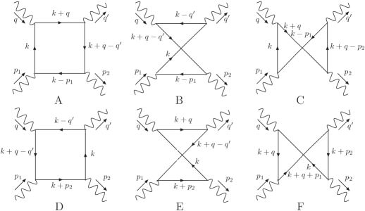
Figure 1: The Born order diagrams for $\gamma^{*}\;\gamma\to\gamma\;\gamma$

Our aim in this section is to calculate this amplitude and present it in the form of an integral over the quark momentum fraction $x$. Since we found this calculation rather instructive, we shall describe with some details how we perform it on the example of the box diagram of Fig. 1A and then exhibit the total result coming from the sum of the six diagrams. For simplicity, we restrict in this short paper to the case where $\Delta_{T}$, the transverse part of $\Delta\doteq p_{2}-p_{1}$, vanishes, that is zero scattering angle (but still non-forward kinematics). We expect to generalize the kinematics in a future work. Our conventions for the kinematics are the following:

$$q=-2\xi p+n\ ,~{}~{}~{}~{}~{}~{}~{}~{}~{}~{}q^{\prime}=n\ ,$$

$$p_{1}=(1+\xi)p\ ,~{}~{}~{}~{}~{}~{}~{}~{}~{}~{}p_{2}=p_{1}+\Delta=(1-\xi)p\ ,$$

where $p$ and $n$ are two light-cone vectors and $2p\cdot n=s=\frac{Q^{2}}{2\xi}$.

The momentum $k$ in the quark loop is chosen to be

$$k^{\mu}\doteq(x+\xi)p^{\mu}+\beta n^{\mu}+k_{T}\ ,$$

with $k_{T}^{2}=-{\mathbb{k}^{2}}$.

The amplitude of the process $\gamma^{*}\gamma\rightarrow\gamma\gamma$ with one virtual and three real photons can be written as

$$A\doteq\,\epsilon_{\mu}\epsilon^{\prime*}_{\nu}{\epsilon_{1}}_{\alpha}{\epsilon^{*}_{2}}_{\beta}T^{\mu\nu\alpha\beta},$$ (2)

where in our kinematics the four photon polarization vectors $\epsilon(q)$, $\epsilon^{\prime*}(q^{\prime})$, $\epsilon_{1}(p_{1})$ and $\epsilon^{*}_{2}(p_{2})$ are transverse. The tensorial decomposition of $T^{\mu\nu\alpha\beta}$ reads [5]

$$T^{\mu\nu\alpha\beta}(\Delta_{T}=0)=\frac{1}{4}g^{\mu\nu}_{T}g^{\alpha\beta}_{T}W_{1}+\frac{1}{8}\left(g^{\mu\alpha}_{T}g^{\nu\beta}_{T}+g^{\nu\alpha}_{T}g^{\mu\beta}_{T}-g^{\mu\nu}_{T}g^{\alpha\beta}_{T}\right)W_{2}+\frac{1}{4}\left(g^{\mu\alpha}_{T}g^{\nu\beta}_{T}-g^{\mu\beta}_{T}g^{\alpha\nu}_{T}\right)W_{3}\,,$$ (3)

and it involves three scalar functions $W_{i}$, $i=1,2,3$.

The integration over $k$ is performed as usual within the Sudakov representation, using

$$d^{4}k=\frac{s}{2}dxd\beta d^{2}k_{T}=\frac{\pi s}{2}dxd\beta d{\mathbb{k}^{2}}$$

Let us present in some details our calculations for diagram A, and afterwards only give final results for the other diagrams. We start with the straightforward calculation of the imaginary part of $W_{i}$ for this diagram. Performing the $d\beta$ and $d{\bf k}^{2}$ integrations with the help of the $\delta$-functions defined by Cutkosky rules, we get for the symmetric $W_{1}$ projection $g^{\mu\nu}_{T}g^{\alpha\beta}_{T}$ :

$$Disc\,W_{1}^{A}=\frac{i}{\pi}e_{q}^{4}N_{C}\int\frac{dx}{x-\xi}\frac{(x^{2}+\bar{x}^{2}-\xi^{2})}{1-\xi^{2}}\;,$$ (4)

where the $x-$integration range is restricted by the positivity conditions attached to the $\delta$-functions, to

$$\xi+\frac{m^{2}}{s}<x<1-\frac{m^{2}}{s}\;.$$ (5)

This leads for this diagram to

$$Disc\,W_{1}^{A}=2i{\cal I}m\,{W}_{1}^{A}=-\frac{i}{\pi}e_{q}^{4}N_{C}\frac{(1-\xi)^{2}}{1-\xi^{2}}\log\frac{m^{2}}{Q^{2}}\;,$$ (6)

where we restricted ourselves to the logarithmic terms and traded $s$ for $Q^{2}$ in the argument of the logarithm.

The corresponding result for the discontinuity of $W_{3}$ attached to the $\mu\leftrightarrow\nu$ antisymmetric tensorial structure is

$$Disc\,W_{3}^{A}=2i{\cal I}m\,W_{3}^{A}=\frac{i}{\pi}e_{q}^{4}N_{C}\frac{(1-\xi)^{2}}{1-\xi^{2}}\log\frac{m^{2}}{Q^{2}}\;,$$ (7)

and the third discontinuity $Disc\,W_{2}^{A}$ vanishes.

The calculation of the real part ${\cal R}e\,W_{1}^{A}$ is more involved. We get for ${\cal R}e\,W_{1}^{A}$

$${\cal R}e\;i\frac{se_{q}^{4}N_{C}}{32\pi^{3}}\int\frac{dx\;d\beta\;d{\mathbb{k}^{2}}\;\;\;TrA_{1}}{[(k+q)^{2}-m^{2}+i\eta][(k-p_{1})^{2}-m^{2}+i\eta](k^{2}-m^{2}+i\eta)[(k+\Delta)^{2}-m^{2}+i\eta]}\,,$$ (8)

where $TrA_{1}=Tr(\gamma_{T}^{\nu}(\hat{k}+\hat{q}+m)\gamma_{T}^{\nu}(\hat{k}+m)\gamma_{T}^{\alpha}(\hat{k}-\hat{p}_{1}+m)\gamma_{T}^{\alpha}(\hat{k}+\hat{q}-\hat{n}+m)\;$.

We first integrate in $\beta$ using the Cauchy theorem. The propagators induce poles in the complex $\beta$-plane with values

$$\beta_{1} = \frac{{\mathbb{k}^{2}}+m^{2}-i\eta}{s(x+\xi)}~{}~{}~{}~{}~{}~{}~{}~{}~{}~{}\beta_{2}=-1+\frac{{\mathbb{k}^{2}}+m^{2}-i\eta}{s(x-\xi)}$$

$$\beta_{3} = \frac{{\mathbb{k}^{2}}+m^{2}-i\eta}{s(x-\xi)}~{}~{}~{}~{}~{}~{}~{}~{}~{}~{}\beta_{4}=\frac{{\mathbb{k}^{2}}+m^{2}-i\eta}{s(x-1)}\;.$$ (9)

Since the four poles are all below the real axis for $x>1$ and all above the real axis for $x<-\xi$, the only region where the amplitude may not vanish is $1>x>-\xi$. In this way we identify two different regions :

• the DGLAP region where $\xi<x<1$, for which one may close the contour in the upper half plane and get the contribution of the pole $\beta_{4}$ ,

• the ERBL region where $-\xi<x<\xi$, for which one may close the contour in the lower half plane and get the contribution of the pole $\beta_{1}$ .

A number of technical simplifications are now helpful. The integral over ${\mathbb{k}^{2}}$ in Eq. (8) is UV divergent. On the other hand, it is a well-known classical result of QED that the sum of integrals corresponding to the six diagrams of Fig. 1 is finite, so we will separate UV divergent terms of each diagram in an algebraic way. One easily verifies that, at the leading logarithmic approximation we are interested in, the trace may be simplified by taking the limit $m^{2}\to 0$. The integral in Eq. (8) may then be written as

$$I^{A}=I^{A}_{4}+I^{A}_{1}=2i\pi\int_{\xi}^{1}dx\,\int\,d{\mathbb{k}^{2}}\frac{TrA_{1}(\beta=\beta_{4})}{DA_{\beta 4}}-2i\pi\int_{-\xi}^{\xi}dx\,\int\,d{\mathbb{k}^{2}}\frac{TrA_{1}(\beta=\beta_{1})}{DA_{\beta 1}}\;,$$ (10)

with the pole values of the propagators :

$$DA_{\beta 4} = \frac{s({\mathbb{k}^{2}}+m^{2})^{2}(1-\xi^{2})((1-\xi)({\mathbb{k}^{2}}+m^{2})+s(1-x)(\xi-x))}{(1-x)^{2}}$$

$$DA_{\beta 1} = \frac{-2s({\mathbb{k}^{2}}+m^{2})^{2}\xi(1+\xi)(2\xi({\mathbb{k}^{2}}+m^{2})+s(\xi^{2}-x^{2}))}{(\xi+x)^{2}}\;.$$

The traces are simple polynomials in ${\mathbb{k}^{2}}$, which may be written as ($i=1,4$) $TrA_{1}(\beta=\beta_{i})\sim\alpha_{i}{\mathbb{k}^{4}}+\gamma_{i}Q^{2}{\mathbb{k}^{2}}+\delta_{i}Q^{4}$. Power counting in ${\mathbb{k}^{2}}$ shows that the $\alpha_{i}{\mathbb{k}^{4}}$ term in these integrals is ultraviolet divergent. Our aim is to recover the UV finiteness of the sum of diagrams before performing the integration over $x$. For this, we simply separate the ultraviolet divergent part of the integrand, $\frac{\alpha_{i}{\mathbb{k}^{4}}}{DA_{\beta i}}$. This yields for the diagram A and the DGLAP region $\xi<x<1$ (at the leading logarithm level)

$$I^{A}_{4}=2i\pi\int_{\xi}^{1}dx\,\int\,d{\bf k}^{2}\frac{TrA^{r}_{1}(\beta=\beta_{4})}{DA_{\beta 4}}+2i\pi\int_{\xi}^{1}dx\int d{\mathbb{k}^{2}}\frac{\alpha_{4}{\mathbb{k}^{4}}}{DA_{\beta 4}}\;,$$ (11)

with the regularized numerator $TrA^{r}_{1}(\beta=\beta_{4})=\gamma_{4}Q^{2}{\mathbb{k}^{2}}+\delta_{4}Q^{4}$. Simple algebra leads then to:

$$I^{A}_{4}=\int_{\xi}^{1}dx\frac{2(x^{2}+(1-x)^{2}-\xi^{2})}{\pi\,s\,(1-\xi^{2})(\xi-x)}\log\frac{m^{2}}{Q^{2}}+2i\pi\int_{\xi}^{1}dx\int d{\mathbb{k}^{2}}\frac{\alpha_{4}{\mathbb{k}^{4}}}{DA_{\beta 4}}\;.$$ (12)

The corresponding result for the ERBL region is

$$I^{A}_{1}=\int_{-\xi}^{\xi}dx\frac{(x+\xi)(\xi-2x+1)}{\pi\,s\,\xi(1+\xi)(x-\xi)}\log\frac{m^{2}}{Q^{2}}+2i\pi\int_{-\xi}^{\xi}dx\int d{\mathbb{k}^{2}}\frac{\alpha_{1}{\mathbb{k}^{4}}}{DA_{\beta 1}}\;.$$ (13)

The same procedure is applied to the five other diagrams of Fig. 1. Diagrams B and C contribute to the same regions $\xi<x<1$ and $-\xi<x<\xi$ as diagram A. Diagrams D, E, F contribute to the ”antiquark” regions $-1<x<-\xi$ and $-\xi<x<\xi$. The results for diagrams B, D and E are similar to the one for diagram A. It is worth emphasizing that diagrams C and F in our leading logarithmic approximation contribute only to the ultraviolet divergent contribution and not to any $\log\frac{m^{2}}{Q^{2}}$ terms. This fact will lead to a handbag dominance interpretation of the leading logarithmic result, as discussed later on.

At this point, we observe that the ultraviolet divergent contributions cancel out, before integration in the $x$ variable, and moreover separately in the two sets of diagrams (A, B, C) and (D, E, F).

The final result of our calculation of the real part of the DVCS amplitude reads

$${\cal R}e\,W_{1} = \frac{e_{q}^{4}\,N_{C}}{2\,\pi^{2}}\int_{-1}^{1}\,dx\frac{2\,x}{(x-\xi)(x+\xi)}\left[\theta(x-\xi)\frac{x^{2}+(1-x)^{2}-\xi^{2}}{1-\xi^{2}}\right.\;$$ (14)

$$+ \left.\theta(\xi-x)\theta(\xi+x)\frac{x(1-\xi)}{\xi(1+\xi)}-\theta(-x-\xi)\frac{x^{2}+(1+x)^{2}-\xi^{2}}{1-\xi^{2}}\;\right]\ln\frac{m^{2}}{Q^{2}}\;.$$

The real parts of $W_{2}$ and $W_{3}$ are calculated in the same way. We get

$${\cal R}e\,W_{2}=0$$ (15)

and

$${\cal R}e\,W_{3} = \frac{e_{q}^{4}\,N_{C}}{2\,\pi^{2}}\int_{-1}^{1}\,dx\frac{2\xi}{(x-\xi)(x+\xi)}\left[\theta(x-\xi)\frac{x^{2}-(1-x)^{2}-\xi^{2}}{1-\xi^{2}}\;\right.$$ (16)

$$- \left.\theta(\xi-x)\theta(\xi+x)\frac{1-\xi}{1+\xi}\;+\theta(-x-\xi)\frac{x^{2}-(1+x)^{2}-\xi^{2}}{1-\xi^{2}}\;\right]\ln\frac{m^{2}}{Q^{2}}\;.$$

The real and imaginary parts of the amplitudes may be put together in the simple form :

$$W_{1} = \frac{e_{q}^{4}\,N_{C}}{2\,\pi^{2}}\int_{-1}^{1}\,dx\frac{2\,x}{(x-\xi+i\eta)(x+\xi-i\eta)}\left[\theta(x-\xi)\frac{x^{2}+(1-x)^{2}-\xi^{2}}{1-\xi^{2}}\;\right.$$ (17)

$$+ \left.\theta(\xi-x)\theta(\xi+x)\frac{x(1-\xi)}{\xi(1+\xi)}-\theta(-x-\xi)\frac{x^{2}+(1+x)^{2}-\xi^{2}}{1-\xi^{2}}\;\right]\ln\frac{m^{2}}{Q^{2}}$$

and

$$W_{3} = \frac{e_{q}^{4}\,N_{C}}{2\,\pi^{2}}\int_{-1}^{1}\,dx\frac{2\xi}{(x-\xi+i\eta)(x+\xi-i\eta)}\left[\theta(x-\xi)\frac{x^{2}-(1-x)^{2}-\xi^{2}}{1-\xi^{2}}\;\right.$$ (18)

$$- \left.\theta(\xi-x)\theta(\xi+x)\frac{1-\xi}{1+\xi}\;+\theta(-x-\xi)\frac{x^{2}-(1+x)^{2}-\xi^{2}}{1-\xi^{2}}\;\right]\ln\frac{m^{2}}{Q^{2}}\;.$$

We now want to interpret this result from the point of view of QCD factorization based on the operator product expansion, yet still in the zeroth order of the QCD coupling constant and in the leading logarithmic approximation. For this, we write for any function ${\cal F}(x,\xi)$ the obvious identity :

$${\cal F}(x,\xi)\;\log\frac{m^{2}}{Q^{2}}={\cal F}(x,\xi)\;\log\frac{m^{2}}{M_{F}^{2}}+{\cal F}(x,\xi)\;\log\frac{M_{F}^{2}}{Q^{2}}\;,$$ (19)

where $M_{F}$ is an arbitrary factorization scale. We will show below that the first term with $\log\frac{m^{2}}{M_{F}^{2}}$ may be identified with the quark content of the photon, whereas the second term with $\log\frac{M_{F}^{2}}{Q^{2}}$ corresponds to the so-called photon content of the photon, coming from the matrix element of the two photon correlator $A_{\mu}(-\frac{z}{2})A_{\nu}(\frac{z}{2})$ which contributes at the same order in $\alpha_{em}$ as the quark correlator to the scattering amplitude. Choosing $M_{F}^{2}=Q^{2}$ will allow to express the DVCS amplitude only in terms of the quark content of the photon.

3 QCD factorization of the DVCS amplitude on the photon

To understand the results of Eqs. (17-18) within the QCD factorization, we first consider two quark non local correlators on the light cone and their matrix elements between real photon states :

$$F^{q}=\int\frac{dz}{2\pi}e^{ixz}\langle\gamma(p^{\prime})|\bar{q}(-\frac{z}{2}N)\gamma.Nq(\frac{z}{2}N)|\gamma(p)\rangle$$ (20)

and

$$\tilde{F}^{q}=\int\frac{dz}{2\pi}e^{ixz}\langle\gamma(p^{\prime})|\bar{q}(-\frac{z}{2}N)\gamma.N\gamma^{5}q(\frac{z}{2}N)|\gamma(p)\rangle$$ (21)

where we note $N=n/n.p$ and where we neglected, for simplicity of notation, both the electromagnetic and the gluonic Wilson lines.

There also exists the photon correlator $F^{N\mu}(-\frac{z}{2}N)F^{\nu N}(\frac{z}{2}N)$ (where $F^{N\mu}=N_{\nu}F^{\nu\mu}$), which mix with the quark operators [1], but contrarily to the quark correlator matrix element, the photonic one begins at order $\alpha_{em}^{0}$, as seen for instance in the symmetric case :

$$\int\frac{dz}{2\pi}e^{ixz}\langle\gamma(p_{2})|F^{N\mu}(-\frac{z}{2}N)F^{\nu N}(\frac{z}{2}N)g_{T\mu\nu}|\gamma(p_{1})\rangle=-g_{T}^{\mu\nu}\epsilon_{\mu}(p_{1})\epsilon^{*}_{\nu}(p_{2})(1-\xi^{2})[\delta(1+x)+\delta(1-x)]\;.$$ (22)

The quark correlator matrix elements, calculated in the lowest order of $\alpha_{em}$ and $\alpha_{S}$, suffer from ultraviolet divergences, which we regulate through the usual dimensional regularization procedure, with $d=4+2\epsilon$. We obtain (with $\frac{1}{\hat{\epsilon}}=\frac{1}{\epsilon}+\gamma_{E}-\log 4\pi$)

$$F^{q}=\frac{N_{C}\,e_{q}^{2}}{4\pi^{2}}g_{T}^{\mu\nu}\epsilon_{\mu}(p_{1})\epsilon^{*}_{\nu}(p_{2})\left[\frac{1}{\hat{\epsilon}}+\log{m^{2}}\right]F(x,\xi)\,,$$ (23)

with

$$F(x,\xi)=\frac{x^{2}+(1-x)^{2}-\xi^{2}}{1-\xi^{2}}\theta(1>x>\xi)-\frac{x^{2}+(1+x)^{2}-\xi^{2}}{1-\xi^{2}}\theta(-\xi>x>-1)+\frac{x(1-\xi)}{\xi+\xi^{2}}\theta(\xi>x>-\xi)$$ (24)

for the $\mu\leftrightarrow\nu$ symmetric (polarization averaged) part. The corresponding results for the antisymmetric (polarized) part read

$$\tilde{F}^{q}=\frac{N_{C}\,e_{q}^{2}}{4\pi^{2}}(-i\epsilon^{\mu\nu pN})\epsilon_{\mu}(p_{1})\epsilon^{*}_{\nu}(p_{2})\left[\frac{1}{\hat{\epsilon}}+\log m^{2}\right]\tilde{F}(x,\xi)$$ (25)

with

$$\tilde{F}(x,\xi)=\frac{x^{2}-(1-x)^{2}-\xi^{2}}{1-\xi^{2}}\theta(1>x>\xi)+\frac{x^{2}-(1+x)^{2}-\xi^{2}}{1-\xi^{2}}\theta(-\xi>x>-1)-\frac{1-\xi}{1+\xi}\theta(\xi>x>-\xi)\;.$$ (26)

Let us stress again that here we concentrate only on the leading logarithmic behaviour and thus focus on the divergent parts and their associated logarithmic functions. The ultraviolet divergent parts are removed through the renormalization procedure involving both quark and photon correlators (see for example [6]). The $\frac{1}{\hat{\epsilon}}$ terms in Eqs. (23, 25) define the non-diagonal element $Z_{\bar{q}q\;FF}$ of the multiplicative matrix of renormalization constants $Z$. The $\frac{1}{\hat{\epsilon}}$ terms are then subtracted by the renormalization of quark operators. The renormalization procedure introduces a renormalization scale which we here identify with a factorization scale $M_{F}$ in the factorized form of the amplitude (see Eq. (30) below). Imposing the renormalization condition that the renormalized quark correlator matrix element vanishes when the factorization scale $M_{F}=m$, we get from Eq. (23) for the renormalized matrix element (20)

$$F^{q}_{R}=\frac{N_{C}\,e_{q}^{2}}{4\pi^{2}}g_{T}^{\mu\nu}\epsilon_{\mu}(p_{1})\epsilon_{\nu}(p_{2})\log{\frac{m^{2}}{M_{F}^{2}}}F(x,\xi)\;,$$ (27)

and a similar result for the antisymmetric case of Eq. (25):

$$\tilde{F}^{q}_{R}=\frac{N_{C}\,e_{q}^{2}}{4\pi^{2}}(-i\epsilon^{\mu\nu pN})\epsilon_{\mu}(p_{1})\epsilon_{\nu}(p_{2})\log{\frac{m^{2}}{M_{F}^{2}}}\tilde{F}(x,\xi)\;.$$ (28)

Eqs. (27, 28) permit us to define the generalized quark distributions in the photon, $H_{i}^{q}(x,\xi,0)$, as

$$F^{q}_{R}=-g_{T}^{\mu\nu}\epsilon_{\mu}(p_{1})\epsilon^{*}_{\nu}(p_{2})H_{1}^{q}(x,\xi,0)\;,\;\;\;\;\tilde{F}^{q}_{R}=i\epsilon^{\mu\nu pN}\epsilon_{\mu}(p_{1})\epsilon^{*}_{\nu}(p_{2})H_{3}^{q}(x,\xi,0)\;.$$ (29)

and to write the quark contribution to the DVCS amplitude as a convolution of coefficient functions and distributions $H_{i}^{q}$

$$W^{q}_{1}=\int\limits_{-1}^{1}dxC_{V}^{q}(x)H_{1}^{q}(x,\xi,0)\;\,,~{}~{}~{}~{}~{}~{}~{}~{}~{}~{}W^{q}_{3}=\int\limits_{-1}^{1}dxC_{A}^{q}(x)H_{3}^{q}(x,\xi,0)\;,$$ (30)

where the Born order coefficient functions $C_{V/A}^{q}$ attached to the quark-antiquark symmetric and antisymmetric correlators are the usual hard process amplitudes :

$$C_{V/A}^{q}=-2e_{q}^{2}\left(\frac{1}{x-\xi+i\eta}\pm\frac{1}{x+\xi-i\eta}\right)\;.$$ (31)

We recover in that way the $\ln\frac{m^{2}}{M_{F}^{2}}$ term in the right hand side of Eq. (19).

The photon operator contribution to the DVCS amplitude at the order $\alpha_{em}^{2}$ considered here, involves a new coefficient function calculated at the factorization scale $M_{F}$, which plays the role of the infrared cutoff, convoluted with the photon correlator (22) or with its antisymmetric counterpart. The results of these convolutions effectively coincide with the amplitudes calculated in Section 2 with the quark mass replaced by the factorization scale $m\to M_{F}$, and leads to the second term in the right hand side of Eq. (19). The triviality of Eq. (19) in fact hides the more general independence of the scattering amplitude on the choice of the scale $M_{F}$ which is controlled by the renormalization group equation.

We still have the freedom to fix the factorization scale $M_{F}^{2}$ in any convenient way. Choosing $M_{F}^{2}=Q^{2}$ kills the logarithmic terms coming from the photon correlator, so that the DVCS amplitude is written (at least, in the leading logarithmic approximation) solely in terms of the quark correlator, recovering a partonic interpretation of the process, see e.g. [7].

4 The GPDs of the photon and their QCD evolution equations

We have thus demonstrated that it is legitimate to define the Born order generalized quark distributions in the photon at zero $\Delta_{T}$ as

$$H_{1}^{q}(x,\xi,0) = \frac{N_{C}\,e_{q}^{2}}{4\pi^{2}}\left[\theta(x-\xi)\frac{x^{2}+(1-x)^{2}-\xi^{2}}{1-\xi^{2}}\;\right.$$ (32)

$$+ \left.\theta(\xi-x)\theta(\xi+x)\frac{x(1-\xi)}{\xi(1+\xi)}\;-\theta(-x-\xi)\frac{x^{2}+(1+x)^{2}-\xi^{2}}{1-\xi^{2}}\right]\;\ln\frac{Q^{2}}{m^{2}}$$

$$H_{3}^{q}(x,\xi,0) = \frac{N_{C}\,e_{q}^{2}}{4\pi^{2}}\left[\theta(x-\xi)\frac{x^{2}-(1-x)^{2}-\xi^{2}}{1-\xi^{2}}\;\right.$$ (33)

$$- \left.\theta(\xi-x)\theta(\xi+x)\frac{1-\xi}{1+\xi}\;+\theta(-x-\xi)\frac{x^{2}-(1+x)^{2}-\xi^{2}}{1-\xi^{2}}\right]\;\ln\frac{Q^{2}}{m^{2}}\;.$$

Since we focussed on the logarithmic factors, we only obtained the anomalous part of these GPDs. Their $x-$ and $\xi-$dependence are shown on Figs. 2 and 3. The $\xi\to 0$ limit of Eqs. (32, 33) leads to the usual anomalous Born order quark content of the photon. The $H_{i}^{q}(x,\xi,0)$ GPDs are continuous functions of $x$ at the points $x=\pm\xi$, but their derivatives are not.

On can verify that these GPDs obey the usual polynomiality conditions

$$\int\,dx\,x^{2p+1}\,H_{1}^{q}(x,\xi,0) \sim \frac{1}{p+1}-\frac{1}{(2p+3)(p+2)}\left[\frac{3p+4}{p+1}\xi^{2p+2}+2\sum_{m=0}^{p}\xi^{2m}\right]\;$$

$$\int\,dx\,x^{2p}\,H_{3}^{q}(x,\xi,0) \sim \frac{2}{2p+1}-\frac{2}{(2p+1)(p+1)}\sum_{m=0}^{p}\xi^{2m}\;,$$ (34)

the other moments vanish.

Figure 2: The unpolarized anomalous photon GPD $H_{1}^{q}/(N_{C}\,e_{q}^{2}/(4\pi^{2})\,\ln\frac{Q^{2}}{m^{2}})$ at Born order and $\Delta_{T}=0$ for $\xi=0$ (full line), $0.1$ (long dashed line), $0.3$ (middle dashed line), $0.5$ (small dashed line).

Figure 3: The polarized anomalous photon GPD $H_{3}^{q}/(N_{C}\,e_{q}^{2}/(4\pi^{2})\,\ln\frac{Q^{2}}{m^{2}})$ at Born order and $\Delta_{T}=0$ for $\xi=0$ (full line), $0.1$ (long dashed line), $0.3$ (middle dashed line) $0.5$ (small dashed line).

Switching on QCD, the photon GPDs evolve from this QED-like parton model result through modified DGLAP-ERBL evolution equations

$$\mu^{2}\,\frac{d}{d\,\mu^{2}}H_{i}^{q}(x,\xi,0)=f_{i}^{q}(x,\xi)+\int\limits_{-1}^{1}\,dx^{\prime}\frac{1}{\xi}\,V_{NS}\left(\frac{x}{\xi},\frac{x^{\prime}}{\xi}\right)H_{i}(x^{\prime},\xi,0)\;,$$ (35)

where $f_{i}^{q}(x,\xi)$ are defined by the r.h.s. of Eqs. (32, 33), as the corresponding functions which multiply $\ln Q^{2}/m^{2}$. The QCD kernel $V_{NS}$ is well-known [8] to the leading order accuracy

$$V_{NS}(x,x^{\prime})=\frac{\alpha_{s}}{4\,\pi}C_{F}\left[\rho(x,x^{\prime})\left[\frac{1+x}{1+x^{\prime}}\left(1+\frac{2}{x^{\prime}-x}\right)\right]+[x\to-x,x^{\prime}\to-x^{\prime}]\right]_{+}$$

$$\rho(x,x^{\prime})=\theta(x^{\prime}\geq x\geq-1)-\theta(x^{\prime}\leq x\leq-1)\;,$$ (36)

with $C_{F}=(N_{C}^{2}-1)/(2N_{C})$. As in the forward case, the presence of the inhomogeneous term allows to fully evaluate the GPDs. We will address this point in a future work.

5 Conclusions

We derived the leading amplitude of the DVCS (polarization averaged or polarized) process on a photon target. We have shown that the amplitude coefficients $W_{i}^{q}$ factorize in the forms shown in Eq. (30), irrespectively of the fact that the handbag diagram interpretation appears only after cancellation of UV divergencies in the scattering amplitude. We have shown that the objects $H_{i}^{q}(x,\xi,t)$ are matrix elements of non-local quark operators on the light cone, and that they have an anomalous component which is proportional to $\log(Q^{2}/m^{2})$. They thus have all the properties attached to generalized parton distributions, and they obey non-homogeneous DGLAP-ERBL evolution equations.

The extension of the results of this work beyond the leading logarithmic approximation requires taking into account the non-pointlike, hadronic contribution of the photon wave function. In the diagonal case of the photon structure function, it is done in a model dependent way, by invoking the vector meson dominance hypothesis (see second Ref. [1]). This approach encounters, however, well known difficulties related to the impossibility to separate in a precise way those non-pointlike contributions from the next to leading order corrections to the processes with the pointlike coupling of the photon [9]. In the non-diagonal case considered here, we may apply a similar strategy and define non-pointlike photon GPDs by relating them to the vector meson GPDs or to the $\gamma\to$ vector meson transition distribution amplitude [10].

References

• [1] E. Witten, Nucl. Phys. B 120 (1977) 189. For a recent review, see M. Klasen, Rev. Mod. Phys.  74 (2002) 1221 and references therein.
• [2] O. V. Teryaev, Phys. Lett. B 510, 125 (2001).
• [3] M. Diehl et.al., Phys. Rev. Lett.  81, 1782 (1998); M. Diehl, T. Gousset and B. Pire, Phys. Rev. D 62, 073014 (2000); B. Pire and L. Szymanowski, Phys. Lett. B 556, 129 (2003).
• [4] B. Pire, J. Soffer and O. Teryaev, Eur. Phys. J. C 8 (1999) 103; P. V. Pobylitsa, Phys. Rev. D 65 (2002) 114015 and Phys. Rev. D 66 (2002) 094002.
• [5] V. M. Budnev, I. F. Ginzburg, G. V. Meledin and V. G. Serbo, Phys. Rept.  15 (1974) 181.
• [6] C. T. Hill and G. G. Ross, Nucl. Phys. B 148 (1979) 373.
• [7] R. J. DeWitt, L. M. Jones, J. D. Sullivan, D. E. Willen and H. W. Wyld, Phys. Rev. D 19 (1979) 2046 [Erratum-ibid. D 20 (1979) 1751].
• [8] D. Müller et al., Fortsch. Phys. 42, 101 (1994); X. Ji, Phys. Rev.  Lett. 78, 610 (1997); Phys.  Rev.  D55, 7114 (1997); A. V. Radyushkin, Phys.  Rev.  D 56, 5524 (1997); J. Blümlein et al., Phys. Lett. B406, 161 (1997). M. Diehl, Phys. Rept. 388, 41 (2003).
• [9] I. Antoniadis and G. Grunberg, Nucl. Phys. B 213 (1983) 445.
• [10] B. Pire and L. Szymanowski, Phys. Rev. D 71, 111501 (2005); J. P. Lansberg, B. Pire and L. Szymanowski, Phys. Rev. D 73, 074014 (2006).