Radiative Kaon Decay in Chiral Perturbation Theory

Abstract

We analyze the possibility of experimental investigation of new low-energy relations between the values of resonance masses in the meson form factors and the differential rate of radiative kaon decay $K^{+}\to\pi^{+}e^{+}e^{-}(\mu^{+}\mu^{-})$ at the current level of the experimental precision. A set of arguments is listed in favour of that these relations can be a consequence of weak static interactions in the Standard Model.

Dedicated to the 70-th anniversary of professor M.K. Volkov

PACS: 11.30Rd, 12.39.Fe, 12.40.Vv, 13.20.Eb, 13.25.Es, 13.75.Lb

The results were presented at

the 5th NA48 Mini-Workshop on kaon physics

(CERN, December 12, 2006).

Introduction

The radiative kaon decay amplitudes $K^{+}\to\pi^{+}e^{+}e^{-}(\mu^{+}\mu^{-})$ are of great interest of the chiral perturbation theory (ChPT) [1, 2, 3] because in the lowest order of ChPT the decay amplitudes are equal to zero [4, 5, 6, 7, 8]. There two opinions about the next order of ChPT.

The first opinion is that in the next order of ChPT the baryon (or quark) loops dominate [4, 6]. As these fermion loops also determine meson form factors in the low energy region [1], in this case, one can supposes that ChPT calculation [1, 2, 3, 4] points out possible relations between the low energy parameters of meson form factors and the differential rates of the radiative kaon decays. These relations can arise if we keep in the ChPT diagrams the real vector meson propagators and take into account the quantum numbers of the nearest resonances in possible vertices [9, 10].

The second opinion is that in ChPT the meson loops dominate. It was shown [5, 7, 8], in the framework of the accepted approach to Standard Model [11, 12, 13] with the point-like approximation of weak interactions, that these meson loops can completely destruct the meson form factor structure of the radiative kaon decay amplitudes in the low energy region.

In this paper, we show that the situation with ChPT for radiative kaon decay amplitudes is more complicate.There are two types of the meson loops. The first of them are provided by the normal ordering of the weak static interactions, and the second are retarded ones.

Recall that static interactions arise in the Hamiltonian approach to the Standard Model (SM) of electroweak (EW) interactions [14, 15] in contrast to the conventional one [11, 12] based on heuristic Lorentz gauge formulation [16, 13], where the static interactions are absent. These static interactions suppress any retarded meson loop contributions [5, 7, 8] that can destruct the meson form factor structure of the decay amplitudes. The meson loop contributions can be only the tadpole loop diagrams following from the normal ordering of the static interaction. This ordering results in an effective action with $\triangle T=1/2$ rule [17, 18] with one unknown parameter $g_{8}$ that can be fixed from other decays as $g_{8}=5.1$. The dominance of weak static interactions justifies the application of low energy chiral perturbation theory [1, 2, 3] as an efficient method of description of kaon decay processes [4, 5, 6, 18].

In this paper we study the possibility of extracting information about the meson form factors from the $K^{+}\to\pi^{+}e(\mu)^{+}e(\mu)^{-}$ processes at the current level of the experimental precision.

The plan of the paper is the following. In Section 1 we present the explicit expressions for amplitudes of the processes $K^{+}\to\pi^{+}l^{+}l^{-}$ in terms of meson form factors. In Section 2 we discuss possibilities of the corresponding experimental tests. Manifestations of the static interactions in decay rates in SM are discussed in Section 3.

1 Relations between form factors and radiative $K$ decay amplitude in ChPT

1.1 Chiral bosonization of EW interaction

It is conventional to describe weak decays in the framework of electroweak (EW) theory at the quark QCD level including current vector boson weak interactions [11, 12]

$$\mathcal{L}_{(J)}=-(J^{-}_{\mu}W^{+}_{\mu}+J^{+}_{\mu}W^{-}_{\mu})=-\frac{e}{2\sqrt{2}\sin\theta_{W}}(\underline{J}^{-}_{\mu}W^{+}_{\mu}+\underline{J}^{+}_{\mu}W^{-}_{\mu}),$$ (1)

where $\underline{J}^{+}_{\mu}=\bar{d}^{\prime}\gamma_{\mu}(1-\gamma_{5})u,$ $\bar{d}^{\prime}=d\cos\theta_{C}+s\sin\theta_{C}$, and $\theta_{C}$ is the Cabbibo angle ($\sin\theta_{C}=0.223$).

However, a consistent theory of QCD at large distances has not been constructed yet. Therefore, the most efficient method of analysis in kaon decay physics [4, 5, 6, 18] is the ChPT [2, 3]. The quark content of $\pi^{+}$ and $K^{+}$ mesons $\pi^{+}=(\bar{d},u),K^{+}=(\bar{s},u),\overline{K}^{0}=(\bar{s},d)$ leads to the effective chiral hadron currents $\underline{J}^{\pm}_{\mu}$ in the Lagrangian (1)

$$\underline{J}^{\pm}_{\mu}=[\underline{J}^{1}_{\mu}{\pm}i\underline{J}^{2}_{\mu}]\cos\theta_{C}\,+[\underline{J}^{4}_{\mu}{\pm}i\underline{J}^{5}_{\mu}]\,\sin\theta_{C}\,,$$ (2)

where using the Gell-Mann matrices $\lambda^{k}$ one can define the meson current as [2]

$$i\sum\limits\lambda^{k}\underline{J}^{k}_{\mu}=i\lambda^{k}(V^{k}_{\mu}-A^{k}_{\mu})^{k}=F^{2}_{\pi}e^{i\xi}\partial_{\mu}e^{-i\xi},$$ (3)

$$\xi=F_{\pi}^{-1}\sum\limits_{k=1}^{8}M^{k}\lambda^{k}=F_{\pi}^{-1}\left(\begin{array}[]{ccc}\pi^{0}+\dfrac{\eta}{\sqrt{3}}&\pi^{+}\sqrt{2}&K^{+}\sqrt{2}\\ \pi^{-}\sqrt{2}&-\pi^{0}+\dfrac{\eta}{\sqrt{3}}&K^{0}\sqrt{2}\\ K^{-}\sqrt{2}&\overline{K}^{0}\sqrt{2}&-\dfrac{2\eta}{\sqrt{3}}\\ \end{array}\right).$$ (4)

In the first orders in mesons one can write

$$V^{-}_{\mu}=\sqrt{2}\,\,[\,\sin\theta_{C}\,(K^{-}\partial_{\mu}\pi^{0}-\pi^{0}\partial_{\mu}K^{-})\,+\cos\theta_{C}\,(\pi^{-}\partial_{\mu}\pi^{0}-\pi^{0}\partial_{\mu}\pi^{-})\,]+...$$ (5)

and

$$A^{-}_{\mu}=\sqrt{2}\,F_{\pi}\,(\partial^{\mu}K^{-}\sin\theta_{C}+\partial^{\mu}\pi^{-}\cos\theta_{C})+...,$$ (6)

here $F_{\pi}\simeq 92.4$ MeV. The right form of the chiral Lagrangian of the electromagnetic interaction of mesons can be constructed by the covariant derivative $\partial_{\mu}\chi^{\pm}\to D_{\mu}\chi^{\pm}\equiv(\partial_{\mu}\pm ieA_{\mu})\chi^{\pm},$ where $\chi^{\pm}=K^{\pm},\pi^{\pm}$.

We suppose also that the quark content of the mesons determines hadronization of QCD [19, 20] conserving its chiral and gauge symmetries.

1.2 The $K^{+}\to\pi^{+}l^{+}l^{-}$ amplitude

Figure 1: $K^{+}\to\pi^{+}\gamma^{*}$ diagrams for effective Lagrangian.

The result of calculation of the amplitude of the process $K^{+}\to\pi^{+}l^{+}l^{-}$ ($l=e;\mu$) in the framework of the chiral Lagrangian (1)–(6) including phenomenological meson form factors denoted by fat dots in Fig. 1 takes the form

$$T_{(K^{+}\to\pi^{+}l^{+}l^{-})}=2g_{8}eG_{\rm EW}L_{\nu}D^{\gamma(rad)}_{\mu\nu}(q)(k_{\mu}+p_{\mu})\,\,\,{\cal T}(q^{2},k^{2},p^{2}),$$ (7)

where $g_{8}=5.1$ is the effective enhancement coefficient [5, 17],

$$G_{\rm EW}=\frac{\sin\theta_{C}\cos\theta_{C}}{8M^{2}_{W}}\frac{e^{2}}{\sin^{2}\theta_{W}}\equiv\sin\theta_{C}\cos\theta_{C}\frac{G_{F}}{\sqrt{2}},$$ (8)

is the coupling constant, $L_{\mu}=\bar{l}\gamma_{\mu}l$ is leptonic current,

$${\cal T}(q^{2},k^{2},p^{2})=F^{2}_{\pi}\left[\frac{f^{V}_{\pi}(q^{2})k^{2}}{m^{2}_{\pi}-k^{2}-i\epsilon}+\frac{f^{V}_{K}(q^{2})p^{2}}{M^{2}_{K}-p^{2}-i\epsilon}+\frac{f^{A}_{K}(q^{2})+f^{A}_{\pi}(q^{2})}{2}\right],$$ (9)

and $f^{(A,V)}_{\pi,K}(q^{2})$ are meson form factors. On the mass-shell the sum (9) takes the form

$${\cal T}(q^{2},M_{K}^{2},m_{\pi}^{2}) =$$ (10)

$$=\leavevmode\nobreak\ {\cal T}(q^{2}) = F^{2}_{\pi}\Bigg{[}\frac{f^{A}_{K}(q^{2})+f^{A}_{\pi}(q^{2})}{2}-f^{V}_{\pi}(q^{2})+\Big{[}f^{V}_{K}(q^{2})-f^{V}_{\pi}(q^{2})\Big{]}\frac{m_{\pi}^{2}}{M_{K}^{2}-m_{\pi}^{2}}\Bigg{]}.$$

The $K^{+}\to\pi^{+}l^{+}l^{-}$ amplitude vanishes at tree level [4, 5], where the form factors are equal to unity: ${\cal T}(q^{2})|_{f^{V}=f^{A}=1}=0$.

In terms of the two standard Dalitz plot variables $q^{2}$ and $t^{2}$ representing the squares of invariant masses of $l^{+}l^{-}$ and $\pi^{+}l^{+}$ pairs, respectively, the amplitude (10) leads to the following decay rate for the transition $K^{+}\to\pi^{+}l^{+}l^{-}$:

$$\Gamma(q^{2},t^{2})=C\int\limits_{4m^{2}_{l}}^{(M_{K}-m_{\pi})^{2}}dq^{2}\cdot|F(q^{2})|^{2}\int\limits_{t_{min}^{2}(q^{2})}^{t_{max}^{2}(q^{2})}dt^{2}\cdot\eta(q^{2},t^{2}),$$ (11)

where

$$\eta(q^{2},t^{2}) = (2t^{2}+q^{2}-2m_{\pi}^{2}-2m_{l}^{2})(2M_{K}^{2}+2m_{l}^{2}-2t^{2}-q^{2})+$$ (12)

$$+q^{2}(q^{2}-2M_{K}^{2}-2m_{\pi}^{2})$$

and

$$F(q^{2}) = \dfrac{(4\pi)^{2}{\cal T}(q^{2})}{q^{2}}=$$ (13)

$$= \frac{(4\pi F_{\pi})^{2}}{q^{2}}\left[\frac{f^{A}_{K}(q^{2})+f^{A}_{\pi}(q^{2})}{2}-f^{V}_{\pi}(q^{2})+\Big{[}f^{V}_{K}(q^{2})-f^{V}_{\pi}(q^{2})\Big{]}\frac{m_{\pi}^{2}}{M_{K}^{2}-m_{\pi}^{2}}\right].$$

The $t^{2}$-dependence does not contain information about the combination of the form factors $F(q^{2})$, which is of our interest. Integration of (11) over $t^{2}$ yields

$$\Gamma(q^{2})=C\int\limits_{4m^{2}_{l}}^{(M_{K}-m_{\pi})^{2}}{\frac{dq^{2}}{M_{K}^{2}}\rho(q^{2})}|F(q^{2})|^{2}.$$ (14)

Here (see [5])

$$C=\frac{(s_{1}c_{1}c_{3})^{2}g_{8}^{2}G^{2}_{F}}{(4\pi)^{4}}\frac{\alpha^{2}M_{K}^{5}}{24\pi}\Big{|}_{g_{8}=5.1}=1.37\times 10^{-22}\leavevmode\nobreak\ \mbox{\rm GeV},$$ (15)

$$\rho(q^{2}) = \left(1-\frac{4m_{l}^{2}}{q^{2}}\right)^{1/2}\left(1+\frac{2m_{l}^{2}}{q^{2}}\right)\leavevmode\nobreak\ \!\lambda^{3/2}(1,q^{2}/M^{2}_{K},m^{2}_{\pi}/M^{2}_{K}),$$

$$\lambda(a,b,c) = a^{2}+b^{2}+c^{2}-2(ab+bc+ca),$$

and $s_{1}c_{1}c_{3}$ is the product of Cabibbo-Kobayashi-Maskawa matrix elements $V_{ud}V_{us}$.

2 Parameterization of $F(q^{2})$

2.1 Parameterization with meson loops

It follows from (13), taking into account $f_{\pi}^{V}(q^{2})\simeq f_{K}^{V}(q^{2})$ and $f_{\pi}^{A}(q^{2})\simeq f_{K}^{A}(q^{2})$:

$$F(q^{2})=\frac{(4\pi F_{\pi})^{2}}{q^{2}}\left[f^{A}(q^{2})-f^{V}(q^{2})\right].$$ (16)

We discuss the differential $K^{+}\to\pi^{+}l^{+}l^{-}$ decay rate (11, 14) in the ChPT [1, 2] with pion and baryon loop contributions leading to meson form factors [1, 4]:

$$\begin{array}[]{ccl}f^{V}(q^{2})&=&1+M^{-2}_{\rho}q^{2}+\alpha_{0}\Pi_{\pi}(q^{2})+...\leavevmode\nobreak\ ;\\ f^{A}(q^{2})&=&1+M^{-2}_{a}q^{2}+...\end{array}$$ (17)

We parameterize the terms linear in $q^{2}$ (determined by the baryon and meson loops [1, 4, 6, 18]) by the values of resonance masses [22] $M_{\rho}=775.8$ MeV, $I^{G}(J^{PC})=1^{+}(1^{--})$ and $M_{a}=984.7$ MeV, $I^{G}(J^{PC})=1^{-}(0^{++})$,

$$\alpha_{0}=\dfrac{4}{3}\cdot\dfrac{m_{\pi}^{2}}{(4\pi F_{\pi})^{2}}=0.01926,$$ (18)

and the nonlinear term of the pion loop contribution [1, 2] is given by

$$\begin{array}[]{rcll}\Pi_{\pi}(t)&=&(1-\bar{t})\left(\dfrac{1}{\bar{t}}-1\right)^{1/2}\arctan\left(\dfrac{\bar{t}^{1/2}}{(1-\bar{t})^{1/2}}\right)-1,&\bar{t}=\dfrac{t}{(2m_{\pi})^{2}}<1;\\ \Pi_{\pi}(t)&=&\dfrac{\bar{t}-1}{2}\left(1-\dfrac{1}{\bar{t}}\right)^{1/2}\left\{i\pi-\log\dfrac{\bar{t}^{1/2}+(\bar{t}-1)^{1/2}}{\bar{t}^{1/2}-(\bar{t}-1)^{1/2}}\right\}-1,&\bar{t}\geq 1.\end{array}$$ (19)

In order to introduce the resonant behavior of the form factors, the following Padé-type approximations [21] to the expressions (17) are considered:

$$\begin{array}[]{rcl}f_{1}^{V}(q^{2})&=&\gamma\left[1-\{M^{-2}_{\rho}q^{2}+\alpha_{0}\cdot\Pi_{\pi}(q^{2})\}/\gamma\right]^{-1}+(1-\gamma),\\ f_{1}^{A}(q^{2})&=&\left(1-M_{a}^{-2}q^{2}\right)^{-1}.\end{array}$$ (20)

Here the parameter $\gamma=0.85$ effectively accounts for higher order loops, and is chosen such as to put the position of maximum of $f_{1}^{V}(q^{2})$ to $q^{2}=M_{\rho}^{2}$.

2.2 Predictions for integrated and differential decay rates

The form factors (20) lead to the following decay branching ratios and muon/electron ratio $R={\rm Br}(K^{+}\to\pi^{+}\mu^{+}\mu^{-})/{\rm Br}(K^{+}\to\pi^{+}e^{+}e^{-})$:

$${\rm Br}(K^{+}\to\pi^{+}e^{+}e^{-})=3.88\times 10^{-7},\leavevmode\nobreak\ \leavevmode\nobreak\ {\rm Br}(K^{+}\to\pi^{+}\mu^{+}\mu^{-})=1.23\times 10^{-7},\leavevmode\nobreak\ \leavevmode\nobreak\ R=0.318.$$

These branching fractions are highly sensitive to the values of $M_{a}$ and $M_{\rho}$ used in the parameterization:

$$\begin{array}[]{ll}\Delta{\rm Br}(ee)/{\rm Br}(ee)\approx 12(\Delta M_{a}/M_{a}),&\Delta{\rm Br}(\mu\mu)/{\rm Br}(\mu\mu)\approx 10(\Delta M_{a}/M_{a}),\\ \Delta{\rm Br}(ee)/{\rm Br}(ee)\approx-20(\Delta M_{\rho}/M_{\rho}),&\Delta{\rm Br}(\mu\mu)/{\rm Br}(\mu\mu)\approx-17(\Delta M_{\rho}/M_{\rho}).\end{array}$$ (21)

However this sensitivity largely cancels in the muon/electron ratio:

$$\Delta R/R\approx-2(\Delta M_{a}/M_{a}),\leavevmode\nobreak\ \leavevmode\nobreak\ \leavevmode\nobreak\ \Delta R/R\approx 2(\Delta M_{\rho}/M_{\rho}).$$

The sensitivity to the parameter $\gamma$ is smaller than to the resonance masses:

$$\Delta{\rm Br}(ee)/{\rm Br}(ee)\approx-0.5(\Delta\gamma/\gamma),\leavevmode\nobreak\ \leavevmode\nobreak\ \Delta{\rm Br}(\mu\mu)/{\rm Br}(\mu\mu)\approx-0.9(\Delta\gamma/\gamma),\leavevmode\nobreak\ \leavevmode\nobreak\ \Delta R/R\approx-0.4(\Delta\gamma/\gamma).$$

Taking into account that the relative uncertainties of resonance masses $M_{a}$ and $M_{\rho}$ that are about 1%, our predictions can be roughly quantified as follows:

$${\rm Br}(K^{+}\to\pi^{+}e^{+}e^{-}) = (3.9\pm 0.8)\times 10^{-7},$$

$${\rm Br}(K^{+}\to\pi^{+}\mu^{+}\mu^{-}) = (1.2\pm 0.3)\times 10^{-7},$$

$$R = 0.32\pm 0.01.$$

Differential rates of $K^{\pm}\to\pi^{\pm}e^{+}e^{-}$ and $K^{\pm}\to\pi^{\pm}\mu^{+}\mu^{-}$ decays corresponding to the parameterization (20) are presented in Fig. 2 along with the rates calculated extrapolating the available experimental data on $K^{\pm}\to\pi^{\pm}e^{+}e^{-}$ decay [23] using a model [8]. Note that the experimentally accessible kinematic region of the $K^{+}\to\pi^{+}e^{+}e^{-}$ decay is limited by a condition $z=q^{2}/M_{K}^{2}\gtrsim(M_{\pi^{0}}/M_{K})^{2}\approx 0.08$, while for the $K^{\pm}\to\pi^{\pm}\mu^{+}\mu^{-}$ decay the whole kinematic range is accessible.

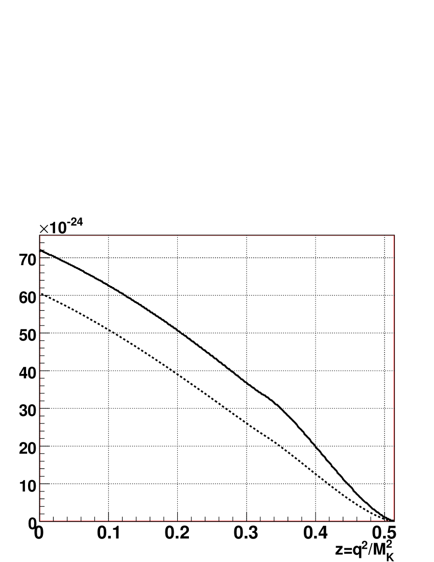
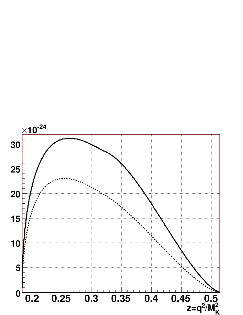
Figure 2: Differential rates of (a) $K^{+}\to\pi^{+}e^{+}e^{-}$ and (b) $K^{+}\to\pi^{+}\mu^{+}\mu^{-}$ decays as functions of $z=q^{2}/M_{K}^{2}$. Solid lines: $F(q^{2})$ parameterization (20); dotted lines: differential distribution measured for $K^{+}\to\pi^{+}e^{+}e^{-}$, $z>0.1$ by [23] and extrapolated for $z<0.1$ and for $K^{+}\to\pi^{+}\mu^{+}\mu^{-}$ using a model [8]. Given the large sensitivity of our calculation to values of $M_{\rho}$ and $M_{a}$, the calculation agrees with the experimental data.

The function $|F(q^{2})|$ determined by the relations (16), (20) is presented in Fig.3. Its shape, being approximated in terms of a linear form factor $F(q^{2})=F_{0}(1+\lambda\cdot q^{2}/M_{K}^{2})$, leads to a form factor varying from a minimum of $\lambda=1.4$ for $z=q^{2}/M_{K}^{2}=0$ to a maximum of $\lambda=4.9$ for a point $z=q^{2}/M_{K}^{2}=0.32$ corresponding to $q^{2}\approx M_{\pi}^{2}$. An effective average form factor slope of the $K^{\pm}\to\pi^{\pm}e^{+}e^{-}$ decay as would be measured by an experiment in the accessible kinematic region $q^{2}>M_{\pi^{0}}^{2}$ is estimated to be $\lambda\approx 2.3$. This value should be subject to variation among different experiments, depending, in particular, on the experimental acceptance as a function of $q^{2}$.

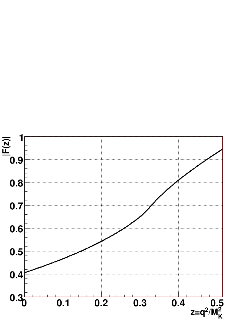
Figure 3: The function $|F(q^{2})|$ determined by the relations (16), (20).

2.3 Prospects for experimental tests

The experimental data for branching fractions, their ratio, and the form factor slope (not considering a slope measurement in the $K^{\pm}\to\pi^{\pm}\mu^{+}\mu^{-}$ channel which is subject to large uncertainties) are [22]:

$${\rm Br}(K^{+}\to\pi^{+}e^{+}e^{-}) = (2.88\pm 0.13)\times 10^{-7},$$

$${\rm Br}(K^{+}\to\pi^{+}\mu^{+}\mu^{-}) = (0.81\pm 0.14)\times 10^{-7},$$

$$R = 0.281\pm 0.050,$$

$$\lambda = 2.14\pm 0.20.$$

The experimental precision of ${\rm Br}(K^{+}\to\pi^{+}e^{+}e^{-})$ is mainly determined by a single measurement [23]. The experimental uncertainty of ${\rm Br}(K^{+}\to\pi^{+}\mu^{+}\mu^{-})$ is dominated by a PDG error scale factor [22] emerging from inconsistency of three measurements [24, 25, 26]. Significant experimental improvements are expected in near future, when the data sample collected by the NA48/2 experiment at CERN is analyzed.

Our predictions for branching fractions of the two decays, their ratio $R$, and the effective form factor slope are in agreement with the experimental data. On the contrary, meson dominance models [27] fail to describe the effective form factor slope, predicting substantially lower slope values.

Monte Carlo simulations involving realistic estimations of experimental conditions show that a deviation of $K^{\pm}\to\pi^{\pm}e^{+}e^{-}$ event distribution predicted by (20) from a distribution corresponding to a linear form factor $F(q^{2})$ (i.e. the predicted dependence of the effective form factor slope $\lambda$ on $q^{2}$) can be experimentally detected with a sample of $\sim 2\cdot 10^{4}$ reconstructed decays, which is not far from the capabilities of the present experiments in terms of kaon flux.

3 Weak static interaction as the origin of enhancement

We listed the set of experimental arguments in favour of that a relation between the form factors and radiative $K$ decay amplitude takes place. In the following part of the paper we would like to show that this relation is not occasional from theoretical point of view.

In any case, we are trying to address the questions: What are contributions of other loop diagrams? What is the origin of the enhancement coefficient $g_{8}$ in the amplitude (7)? What is origin of the coincidence of the resonance parameters with the kaon decay ones?

We show below that a reply to all these questions can be the weak static interaction as a consequence of Dirac like radiation variables in SM.

3.1 The Radiation Variables in Standard Model

As it was shown by Dirac in QED [28], the static interactions in gauge theories are an inevitable consequence of the general principles of QFT, including the vacuum postulate. In order to obtain a physical vacuum as a state with minimal energy, Dirac eliminated all zero momentum fields (with their possible negative contributions into the energy of the system) by solving the Gauss constraint and dressing charged fields by the phase factors (see also [29, 30, 31]). This elimination leads to the radiation variables and the static interactions in both QED and the massive vector boson theory [14].

In particular, in QED the radiation gauge-invariant variables $A^{(\rm R)}_{\mu}(A)=A_{\mu}-\partial_{\mu}\dfrac{1}{\triangle}(\partial_{k}A^{k})$ have propagators $\widetilde{J}^{+}_{\mu}D^{\rm R}_{\mu\nu}(q)\widetilde{J}^{-}_{\nu}=\dfrac{\widetilde{J}^{+}_{0}\widetilde{J}^{-}_{0}}{\vec{q}^{2}}+\left(\delta_{ij}-\dfrac{q_{i}q_{j}}{\vec{q}^{2}}\right)\dfrac{\widetilde{J}^{+}_{i}\widetilde{J}^{-}_{j}}{q^{2}}$; while the Lorentz ones $A^{(\rm L)}_{\mu}(A)=A_{\mu}-\partial_{\mu}\dfrac{1}{\Box}(\partial_{\nu}A^{\nu})$ [13] have propagators $\widetilde{J}_{\mu}^{+}D^{L}_{\mu\nu}(q)\widetilde{J}_{\nu}^{-}=-\widetilde{J}_{\mu}^{+}\dfrac{1}{q^{2}}\left(g_{\mu\nu}-\dfrac{q_{\mu}q_{\nu}}{\Box}\right)\widetilde{J}_{\nu}^{-}$.

In order to demonstrate the inequivalence between the radiation variables and the Lorentz ones, let us consider the electron-positron scattering amplitude $T^{R}=\langle e^{+},e^{-}|\hat{S}|e^{+},e^{-}\rangle$. One can see that the Feynman rules in the radiation gauge give the amplitude in terms of the current $j_{\nu}=\!\bar{e}\gamma_{\nu}e$

$$T^{R}=\frac{J^{2}_{0}}{\mathbf{q}^{2}}+\left(\delta_{ik}-\dfrac{q_{i}q_{k}}{\mathbf{q}^{2}}\right)\frac{J_{i}J_{k}}{q^{2}+i\varepsilon}\equiv\frac{-J^{2}}{q^{2}+i\varepsilon}+\framebox{$\dfrac{(q_{0}J_{0})^{2}-(\mathbf{q}\cdot\mathbf{j})^{2}}{\mathbf{q}^{2}[q^{2}+i\varepsilon]}$}\leavevmode\nobreak\ .$$ (22)

This amplitude coincides with the Lorentz gauge one,

$$T^{L}=-\frac{1}{q^{2}+i\varepsilon}\left[J^{2}-\framebox{$\dfrac{(q_{0}J_{0}-\mathbf{q}\cdot\mathbf{J})^{2}}{q^{2}+i\varepsilon}$}\,\,\right]\leavevmode\nobreak\ ,$$ (23)

when the box terms in Eq. (22) can be eliminated. Thus, the Faddeev equivalence theorem [30] is valid, if the currents are conserved

$$q_{0}{J}_{0}-\mathbf{q}\cdot\mathbf{J}=qJ=0,$$ (24)

and the box terms are eliminated. It just the case, when the R variables are equivalent to the L ones [30]. However, if elementary particles are off their mass-shell (in particular, in bound states) the currents are not conserved.

Radiation variables have vacuum as a state with the minimal energy, whereas the Lorentz ones lose the vacuum postulate as the time component give the negative contribution into the energy. Therefore, Schwinger in [29] … rejected all Lorentz gauge formulations as unsuited to the role of providing the fundamental operator quantization …

Let we believe Schwinger, and consider the massive vector Lagrangian

$${\cal L}=-\frac{1}{2}(\partial_{\mu}W_{\nu}^{+} - \partial_{\nu}W_{\mu}^{+})(\partial_{\mu}W_{\nu}^{-}-\partial_{\nu}W_{\mu}^{-})+M^{2}_{W}W_{\mu}^{+}W_{\mu}^{-}+$$

$$+ \left[J^{-}_{\mu}W_{\mu}^{+}+J^{+}_{\mu}W_{\mu}^{-}\right]\frac{e}{2\sqrt{2}\sin\theta_{W}}$$

in terms of radiation variables [14] $W^{\pm R}_{\mu}=W^{\pm}_{\mu}+\partial_{\mu}[{1}/{(M_{W}^{2}-\triangle)}]\partial_{k}W^{\pm}_{k}$

In this case, instead of the standard propagator [13]

$$\widetilde{J}_{\mu}^{+}D^{L}_{\mu\nu}(q)\widetilde{J}_{\nu}^{-}=-\widetilde{J}_{\mu}^{+}\frac{1}{q^{2}-M_{W}^{2}}\left(g_{\mu\nu}-\frac{q_{\mu}q_{\nu}}{M_{W}^{2}}\right)\widetilde{J}_{\nu}^{-}$$ (25)

we have the radiation one [14]

$$\widetilde{J}^{+}_{\mu}D^{\rm R}_{\mu\nu}(q)\widetilde{J}^{-}_{\nu}=\framebox{$\dfrac{\widetilde{J}^{+}_{0}\widetilde{J}^{-}_{0}}{\vec{q}^{2}+M_{W}^{2}}$}+\left(\delta_{ij}-\frac{q_{i}q_{j}}{\vec{q}^{2}+M_{W}^{2}}\right)\frac{\widetilde{J}^{+}_{i}\widetilde{J}^{-}_{j}}{q^{2}-M_{W}^{2}}$$ (26)

The R–propagator is regular in the limit $M_{W}\rightarrow 0$ and is well behaved for large momenta. In the following we compare two propagators $D_{\mu\nu}^{L}$ and $D_{\mu\nu}^{R}$.

3.2 Weak static interaction as the origin of enhancement

Figure 4: Axial (a) and vector (b) current contribution into $K^{+}\to\pi^{+}$ transition

Let us consider the $K^{+}\to\pi^{+}$ transition amplitude

$$\langle\pi^{+}|-i\int dx^{4}dy^{4}J^{\mu}(x)D_{\mu\nu}^{W}(x-y)J^{\nu}(y)|K^{+}\rangle=i(2\pi)^{4}\delta^{4}(k-p)G_{\rm EW}\Sigma(k^{2}),$$ (27)

in the first order of the EW perturbation theory in the Fermi coupling constant (8) comparing two different W-boson field propagators, the accepted Lorentz (L) propagator (25) and the radiation (R) propagator (26).These propagators give the expressions corresponding to the diagrams in Fig. 4

$$\Sigma(k^{2}) \to \Sigma^{R}(k^{2})=2F^{2}_{\pi}{k^{2}}+2i\int\frac{d^{4}q{M_{W}^{2}}}{(2\pi)^{4}}\frac{k^{2}+(k_{0}+q_{0})^{2}}{(-|\vec{q}|^{2}-M_{W}^{2})[(k+q)^{2}-m^{2}_{\pi}+i\epsilon]},$$ (28)

$$\Sigma(k^{2}) \to \Sigma^{L}(k^{2})=2F^{2}_{\pi}{k^{2}}+2i\int\frac{d^{4}q{M_{W}^{2}}}{(2\pi)^{4}}\frac{(2k_{\mu}+q_{\mu})D^{L}_{\mu\nu}(-q)(2k_{\nu}+q_{\nu})}{(k+q)^{2}-m^{2}_{\pi}+i\epsilon}.$$ (29)

The versions R and L coincide in the case of the axial contribution corresponding to the first diagram in Fig. 4, and they both reduce to the static interaction contribution because

$$k^{\mu}k^{\nu}D^{F}_{\mu\nu}(k)\equiv k^{\mu}k^{\nu}D^{R}_{\mu\nu}(k)=\frac{k_{0}^{2}}{M^{2}_{W}}.$$

However, in the case of the vector contribution corresponding to the second diagram in Fig. 4 the radiation version differs from the Lorentz gauge version (25).

In contrast to the Lorentz gauge version (25), two radiation variable diagrams in Fig. 4 in the rest kaon frame $k_{\mu}=(k_{0},0,0,0)$ are reduced to the static interaction contribution

$$i(2\pi)^{4}\delta^{4}(k-p)G_{\rm EW}\Sigma^{R}(k^{2})=\langle\pi^{+}|-i\int dx^{4}J_{0}(x)\frac{1}{\triangle-M_{W}^{2}}J_{0}(x)|K^{+}\rangle$$ (30)

with the normal ordering of the pion fields which are at their mass-shell, so that

$$\Sigma^{R}(k^{2})=2k^{2}{F^{2}_{\pi}}\left[1+\frac{M_{W}^{2}}{F^{2}_{\pi}(2\pi)^{3}}\int\frac{d^{3}l}{2E_{\pi}(\vec{l})}\frac{1}{M^{2}_{W}+\vec{l}^{2}}\right]\equiv 2k^{2}{F^{2}_{\pi}}g_{8}.$$ (31)

Here $E_{\pi}(\vec{l})=\sqrt{m^{2}_{\pi}+\vec{l}^{2}}$ is the energy of $\pi$-meson and $g_{8}$ is the parameter of the enhancement of the probability of the axial $K^{+}\to\pi^{+}$ transition. The pion mass-shell justifies the application of the low-energy ChPT [1], where the summation of the chiral series can be considered here as the meson form factors [4, 6, 18] $\int\dfrac{d^{3}l}{2E_{\pi}(\vec{l})}\to$ $\int\dfrac{d^{3}lf^{V}_{K}(-(\vec{l})^{2})f^{V}_{\pi}(-(\vec{l})^{2})}{2E_{\pi}(\vec{l})}$.

Using the covariant perturbation theory [32] developed as the series $\underline{J}_{\mu}^{k}(\gamma\oplus\xi)=\underline{J}_{\mu}^{k}(\xi)+F^{2}_{\pi}\partial_{\mu}\gamma^{k}+\gamma^{i}f_{ijk}\underline{J}_{\mu}^{j}(\xi)+O(\gamma^{2})$ with respect to quantum fields $\gamma$ added to $\xi$ as the product $e^{i\gamma}e^{i\xi}\equiv e^{i(\gamma\oplus\xi)}$, one can see that the normal ordering

$$<0|\gamma^{i}(x)\gamma^{i^{\prime}}(y)|0>=\delta^{ii^{\prime}}N(\vec{z}),\leavevmode\nobreak\ \leavevmode\nobreak\ \leavevmode\nobreak\ \leavevmode\nobreak\ N(\vec{z})=\int\frac{d^{3}le^{i\vec{l}\cdot(\vec{z})}}{(2\pi)^{3}2E_{\pi}(\vec{l})},$$

where $\vec{z}=\vec{x}-\vec{y}$, in the product of the currents $\underline{J}_{\mu}^{k}(\gamma\oplus\xi)$ leads to an effective Lagrangian with the rule $\triangle T=1/2$

$$M_{W}^{2}\int d^{3}zg_{8}(|z|)\frac{e^{-M_{W}|\vec{z}|}}{4\pi|\vec{z}|}[\underline{J}_{\mu}^{j}(\xi(x))\underline{J}_{\mu}^{j^{\prime}}(\xi(z+x))(f_{ij1}+if_{ij2})(f_{i^{\prime}j^{\prime}4}-if_{i^{\prime}j^{\prime}5})\delta^{ii^{\prime}}+h.c],$$

where $g_{8}(|z|)=[1+\sum\limits_{I\geq 1}c^{I}N^{I}(\vec{z})]$ is series over the multipaticle intermediate states (this sum is known as the Volkov superpropagator [2, 33]). In the limit $M_{W}\to\infty$, in the lowest order with respect to $M_{W}$, the dependence of $g_{8}(|\vec{z}|)$ and the currents on $\vec{z}$ disappears in the integral of the type of

$$M^{2}_{W}\int d^{3}z\dfrac{g_{8}(|\vec{z}|)e^{-M_{W}|\vec{z}|}}{4\pi|\vec{z}|}=\int_{0}^{\infty}drre^{-r}g_{8}({r}/{M_{W}})\simeq g_{8}(0).$$

In the next order, the amplitudes $K^{0}(\bar{K}^{0})\to\pi^{0}$ arise. Finally, we get the effective Lagrangians [17]

$$\mathcal{L}_{(\Delta T=\frac{1}{2})}=\frac{G_{F}}{\sqrt{2}}g_{8}(0)\cos\theta_{C}\sin\theta_{C}\Big{[}(\underline{J}^{1}_{\mu}+i\underline{J}^{2}_{\mu})(\underline{J}^{4}_{\mu}-i\underline{J}^{5}_{\mu})-(\underline{J}^{3}_{\mu}+\frac{1}{\sqrt{3}}\underline{J}^{8}_{\mu})(\underline{J}^{6}_{\mu}-i\underline{J}^{7}_{\mu})+h.c.\Big{]},$$ (32)

$$\mathcal{L}_{(\Delta T=\frac{3}{2})}=\frac{G_{F}}{\sqrt{2}}\cos\theta_{C}\sin\theta_{C}\Big{[}(\underline{J}^{3}_{\mu}+\frac{1}{\sqrt{3}}\underline{J}^{8}_{\mu})(\underline{J}^{6}_{\mu}-i\underline{J}^{7}_{\mu})+h.c.\Big{]}.$$ (33)

This result shows that the enhancement can be explained by static vector interaction that increases the $K^{+}\to\pi^{+}$ transition by a factor of $g_{8}=g_{8}(0)$, and yields a new term describing the $K^{0}\to\pi^{0}$ transition proportional to $g_{8}-1$.

This Lagrangian with the fit parameter $g_{8}=5$ (i.e. $g_{8}\sin\theta_{C}\cos\theta_{C}\simeq 1$) describes the nonleptonic decays in satisfactory agreement with experimental data [2, 17].

Conclusions

We have investigated the low-energy relations between the values of resonance masses in the meson form factors, and the differential radiative kaon decay $K^{+}\to\pi^{+}e^{+}e^{-}(\mu^{+}\mu^{-})$ rates following from the ChPT [1, 2, 4]. We give non-trivial predictions of muon/electron ratio and the effective form factor slope, which are in agreement with the experimental data.

The high sensitivity of these relations, the low energy status of ChPT, where they arise, and the universality of the enhancement coupling constant $g_{8}$ for all kaon–pion weak transition amplitudes with the rule of selection $\triangle T=1/2$ can be explained by a weak static interaction of massive vector bosons in the Hamiltonian approach to SM [14].

The instantaneous character of weak static interaction in the Hamiltonian SM excludes all retarded diagram contribution in the effective Chiral Perturbation Theory [8] that destruct the form factor structure of the kaon radiative decay rates. The enhancement of kaon–pion transition can be considered as a consequence of normal ordering of all pions in the instantaneous loop on their mass-shells $p^{2}=m^{2}_{\pi}$. The static interaction mechanism of the enhancement of the $\triangle T=1/2$ transitions predicts the coincidence of the meson form factor resonance parameters with the parameters of the radiation kaon decay rates $K^{+}\to\pi^{+}e^{+}e^{-}(\mu^{+}\mu^{-})$ in satisfactory agreement with the experimental data [22, 23].

Therefore, the off-mass-shell kaon-pion transition in the radiation weak kaon decays can be a good probe of the weak static interactions.

Appendix A Appendix A: Calculation of $K^{+}\to\pi^{+}l^{+}l^{-}$ Decay Width

A.1 The Matrix Element

Figure 5: $K^{+}\to\pi^{+}l^{-}l^{+}$ diagram.

The matrix element for the process in Fig. 5 can be obtained by Feynman rules:

$$i\mathcal{M}(K^{+}\to\pi^{+}l^{+}l^{-})=\bar{u}^{s}(q_{-})(-ie\gamma^{\mu})v^{s^{\prime}}(q_{+})\ i\frac{g_{\mu\nu}}{q^{2}}\ <\pi^{+}(p)|J_{em}{{}^{\nu}}|K^{+}(k)>,$$ (34)

after inserting parametrization

$$i\mathcal{M}(K^{+}\to\pi^{+}l^{+}l^{-})=\bar{u}^{s}(q_{-})(-ie\gamma^{\mu})v^{s^{\prime}}(q_{+})\ i\frac{g_{\mu\nu}}{q^{2}}\ eF(kp)(k+p)^{\nu}.$$ (35)

To obtain the square root of matrix element one has to sum over spins

$$\sum_{s,s^{\prime}}|\mathcal{M}|^{2} = \frac{e^{4}|F(kp)|^{2}}{q^{4}}Tr[q_{+}\!\!\!\!/\gamma_{\mu}\!\!\!\!/q_{-}\!\!\!\!/\gamma_{\nu}\!\!\!\!/-m^{2}_{l}\gamma_{\mu}\!\!\!\!/\gamma_{\nu}\!\!\!\!/](p+k)^{\mu}(p+k)^{\nu}$$ (36)

$$= \frac{4e^{4}|F(kp)|^{2}}{q^{4}}[q_{+\mu}q_{-\nu}+q_{+\nu}q_{-\mu}-q_{+}q_{-}g_{\mu\nu}-m^{2}_{l}g_{\mu\nu}](p+k)^{\mu}(p+k)^{\nu}$$

$$= \frac{4e^{4}|F(kp)|^{2}}{q^{4}}[2q_{+}(p+k).q_{-}(p+k)-q_{+}q_{-}(p+k)^{2}-m^{2}_{l}(p+k)^{2}].$$

Next if we define

$$z=\frac{q^{2}}{M_{K}^{2}}=\frac{2q_{+}q_{-}+2m^{2}_{l}}{M_{K}^{2}};\quad x=\frac{(p+q_{-})^{2}}{M_{K}^{2}}=\frac{m_{\pi}^{2}+2pq_{-}+m^{2}_{l}}{M_{K}^{2}};\quad R=\Big{(}\frac{m_{\pi}}{M_{K}}\Big{)}^{2};r_{l}=\Big{(}\frac{m_{l}}{M_{K}}\Big{)}^{2},$$ (37)

where $l=e,\mu$ one obtains

$$\sum|\mathcal{M}|^{2}(z,x) = \frac{2e^{4}F^{2}}{z^{2}}\Big{[}\Big{(}2x+z-2-2r_{l}\Big{)}\Big{(}-2x-z+2R+2r_{l}\Big{)}+z\Big{(}z-2-2R\Big{)}\Big{]},$$

where we used momentum conservation law and relations:

$$k=p+q_{-}+q_{+}=p+q,$$

$$q_{-}q_{+}=\frac{M_{K}^{2}}{2}(z-2r),$$

$$(k+p)^{2}=M_{K}^{2}(2+2R-z),$$

$$(k-p)^{2}=q^{2}=M_{K}^{2}z,$$

$$q_{-}(p+k)=\frac{M_{K}^{2}}{2}(2x+z-2R-2r),$$

$$q_{+}(p+k)=\frac{M_{K}^{2}}{2}(2+2r-z-2x),$$

$$q(p+k)=M_{K}^{2}(1-R).$$

A.2 The decay rate

The phase volume (in the frame of $\vec{k}=0$) is

$$d\Phi = \frac{d^{3}q_{+}d^{3}q_{-}d^{3}p}{2\epsilon_{+}2\epsilon_{-}2\epsilon}\delta^{4}(k-p-q_{+}-q_{-});\qquad\quad d^{4}q_{-}=d^{4}q,$$ (38)

$$= \frac{|\vec{q}_{+}|\epsilon_{+}d\epsilon_{+}d\Omega_{+}}{2\epsilon_{+}}d^{4}qd^{4}p\delta^{4}(k-p-q)\delta((k-q)^{2}-m_{\pi}^{2})\delta((q-q_{+})^{2}-m_{l}^{2}),$$

$$= \frac{|\vec{q}_{+}|d\epsilon_{+}d\Omega_{+}}{2.2M_{K}}\frac{1}{2}|\vec{q}|dq^{2}4\pi\delta\Big{(}q^{2}-2q_{+}q\Big{)};\qquad d\Omega_{+}=2\pi d\cos\theta_{+},$$

$$= \frac{d\epsilon_{+}}{8M_{K}}4\pi dq^{2}\frac{1}{2}2\pi=\frac{dxdz}{16}4\pi 2\pi M_{K}^{2};\qquad q_{+}q=q_{0}\epsilon_{+}-|\vec{q}||\vec{q}_{+}|\cos\theta_{+},$$

and the decay width is

$$d\Gamma = \frac{1}{2M_{K}}\frac{2e^{4}F^{2}}{z^{2}}\Big{[}\Big{(}2x+z-2-2r_{l}\Big{)}\Big{(}-2x-z+2R+2r_{l}\Big{)}+z\Big{(}z-2-2R\Big{)}\Big{]}$$ (39)

$$\times \frac{1}{(2\pi)^{5}}\frac{dxdz}{4}\pi^{2}M_{K}^{2}.$$

$$\frac{d\Gamma}{M_{K}dxdz}=\frac{\alpha^{2}F^{2}}{8\pi z^{2}}\Big{[}\Big{(}2x+z-2-2r_{l}\Big{)}\Big{(}-2x-z+2R+2r_{l}\Big{)}+z\Big{(}z-2-2R\Big{)}\Big{]}.$$

After integration the decay width is

$$\frac{d\Gamma}{M_{K}dz}=\frac{\alpha^{2}}{6\pi z^{3}}\lambda^{\frac{3}{2}}(1,z,R)F^{2}(z)(z+2r)\sqrt{1-\frac{4r}{z}},$$ (40)

where

$$\lambda(1,z,R)=(z^{2}+1+R^{2}-2z-2Rz-2R).$$ (41)

References

• [1] M. Volkov, V. Pervushin, Phys. Lett. B51, 356 (1974).
• [2] M. K. Volkov and V. N. Pervushin, Usp. Fiz. Nauk 120, 363 (1976).
M. K. Volkov and V. N. Pervushin, ‘‘Essentially Nonlinear Field Theory, Dynamical Symmetry and Pion Physics’’, Atomizdat, Moscow, ed. D.I. Blokhintsev, 1979 (in Russian).
• [3] J. Gasser and H. Leutwyler, Ann. of Phys. 158, 142 (1984).
• [4] A.A. Bel’kov, Yu. L. Kalinovsky, V. N. Pervushin, JINR-P2-85-107 (1985).
A.A. Bel’kov et al., Yad. Fis. 44, 690 (1986).
• [5] G. Ecker et al., Nucl. Phys. B291, 692 (1987).
• [6] A.A. Bel’kov et al., Phys. Part. Nucl. 26, 239 (1995).
A.A. Bel’kov, Phys. Part. Nucl. 36, 509 (2005).
• [7] G. Ecker, Prog. Part. Nucl. Phys. 36, 71 (1996); hep-ph/9511412.
• [8] G. D’Ambrosio et al., JHEP 9808, 4 (1998).
• [9] A.Z. Dubničková et al., JINR E2-2006-80, Dubna, 2006; hep-ph/0606005.
• [10] A.Z. Dubničková et al., hep-ph/0611175.
• [11] G. Altarelli and L. Maiani, Phys. Lett. 52B, 351 (1974).
M.K. Gaillard and B.W. Lee, Phys. Rev. Lett. 33, 108 (1974).
• [12] A.I. Vainshtein et al., Yad. Fiz. 24, 820 (1976).
S.S. Gershtein and M. Yu. Khlopov, JETP Lett. 23, 338 (1976).
• [13] D. Bardin and G. Passarino, ‘‘The standard model in the making: precision study of the electroweak interactions’’, Clarendon, Oxford, 1999.
• [14] H.-P. Pavel and V. N. Pervushin, Int. J. Mod. Phys. A14, 2885 (1999).
• [15] B. M. Barbashov et al., hep-th/0611252.
• [16] L. Faddeev and V. Popov, Phys. Lett. B25, 29 (1967).
• [17] Yu.L. Kalinovsky, V.N. Pervushin, Sov. J. Nucl. Phys., 29, 225 (1979).
• [18] A.A. Bel’kov et al., Phys. Lett. B220, 459 (1989).
• [19] Yu.L. Kalinovsky et al., Sov. J. Nucl. Phys. 49, 1059 (1989).
V.N. Pervushin, Nucl. Phys. B (Proc. Supp.) 15, 197 (1990).
• [20] V.N. Pervushin, Phys. Part. Nucl. 34, 348 (2003).
• [21] H. Lehmann, Phys. Lett. 41, 529 (1972).
J. Honerkamp, Nucl. Phys. B36, 130 (1972).
G. Ecker and J. Honerkamp, Nucl. Phys. B52, 211 (1973).
M.K. Volkov and V.N. Pervushin, Nuovo Cimento A27, 277 (1975).
• [22] W.-M. Yao et al. (PDG), J. Phys. G33, 1 (2006).
• [23] R. Appel et al., Phys. Rev. Lett. 83, 4482 (1999).
• [24] S. Adler et al., Phys. Rev. Lett. 79, 4756 (1997).
• [25] H. Ma et al., Phys. Rev. Lett. 84, 2580 (2000).
• [26] H.K. Park et al., Phys. Rev. Lett. 88, 111801 (2002).
• [27] P. Lichard, Phys. Rev. D60, 053007 (1999).
• [28] P.A.M. Dirac, Proc. Roy. Soc. A 114, 243 (1927), Can. J. Phys. 33, 650 (1955).
• [29] J. Schwinger, Phys. Rev. 127, 324 (1962).
• [30] L. Faddeev, T. M. F. 1, 3 (1969).
• [31] N.P. Ilieva, N.S. Han, V.N. Pervushin, Sov. J. Nucl. Phys. 45, 1169 (1987).
N.S. Han, V.N. Pervushin, Mod. Phys. Lett. A2, 367 (1987).
V.N. Pervushin, Nucl. Phys. B (Proc. Supp.) 15, 197 (1990).
• [32] V.N. Pervushin, Theor. Math. Phys. 27, 330 (1977).
D.I. Kazakov, V.N. Pervushin, S.V. Pushkin, J. Phys. A. Math. Gen. 11, 2093 (1978).
• [33] M.K. Volkov, Ann. Phys. (N. Y.) 49, 202 (1968).
C.J. Isham, Abdus Salam, and J. Strathdee, Phys. Rev. D3, 1805 (1971).