Gluon-induced $W$-boson pair production at the LHC

Abstract:

Pair production of $W$ bosons constitutes an important background to Higgs boson and new physics searches at the Large Hadron Collider LHC. We have calculated the loop-induced gluon-fusion process $gg\to W^{*}W^{*}\to{\rm leptons}$, including intermediate light and heavy quarks and allowing for arbitrary invariant masses of the $W$ bosons. While formally of next-to-next-to-leading order, the $gg\to W^{*}W^{*}\to{\rm leptons}$ process is enhanced by the large gluon flux at the LHC and by experimental Higgs search cuts, and increases the next-to-leading order $WW$ background estimate for Higgs searches by about $30\%$. We have extended our previous calculation to include the contribution from the intermediate top-bottom massive quark loop and the Higgs signal process. We provide updated results for cross sections and differential distributions and study the interference between the different gluon scattering contributions. We describe important analytical and numerical aspects of our calculation and present the public GG2WW event generator.

1 Introduction

Vector-boson pair production provides an important background to Higgs boson searches in the $pp\to H\to W^{\ast}W^{\ast}\to{\rm leptons}$ channel at the Large Hadron Collider (LHC). Since for dileptonic $W$ decays no Higgs mass peak can be reconstructed, this background cannot be estimated from measured data via sideband interpolation. Precise theoretical predictions for the irreducible $W$-pair continuum background are hence crucial.

The hadronic production of $W$ pairs has been investigated extensively in the literature (see e.g. Ref. [1]). The next-to-leading order (NLO) QCD corrections to $q\bar{q}\to WW\to\ell\bar{\nu}\bar{\ell^{\prime}}\nu^{\prime}$ have been known for some time [2, 3, 4, 5, 6]. More recently also single-resonant contributions have been included [7], and the NLO calculation has been matched with a parton shower [8] and combined with a summation of soft-gluon effects [9]. Electroweak corrections, which become important at large $WW$ invariant masses, have been computed in Ref. [10].

In this article we present the first complete calculation of the gluon-induced process $gg\to W^{*}W^{*}\to{\rm leptons}$ and study its importance as a background to Higgs searches in the $pp\to H\to WW\to\ell^{+}\ell^{-}p\hskip-5.03125pt\hbox to5.03125pt{\hss$/$\hss}_{T}$ channel. The gluon-induced background process is mediated by quark loops and thus suppressed by two powers of $\alpha_{\rm s}$ relative to quark-antiquark annihilation. Although it formally enters only at next-to-next-to-leading order, the importance of the gluon-fusion process is enhanced by experimental Higgs search cuts. These cuts exploit the longitudinal boost and the spin correlations of the $WW$ system to suppress $W$-pair continuum production through quark-antiquark annihilation [11, 12].

The gluon-fusion contribution to on-shell $W$-pair production, $gg\to WW$, has been computed in Refs. [13, 14, 15]. Here, we present a fully differential calculation of gluon-induced $W$-boson pair production and decay, $gg\to W^{\ast}W^{\ast}\to\ell\bar{\nu}\bar{\ell^{\prime}}\nu^{\prime}$, including the top-bottom massive quark loop contribution and the intermediate Higgs contribution with full spin and decay angle correlations and allowing for arbitrary invariant masses of the $W$ bosons. Partial results of this work have already been presented in Refs. [20, 21]. In Ref. [20] we found that the contributions of the first and second quark generations enhance the NLO $WW$ background prediction for Higgs searches by approximately $30\%$.

In the following we describe details of our calculation, introduce the GG2WW program and present cross sections and differential distributions. We discuss the impact of the third-generation contribution and interference effects between massless and massive quark loop as well as signal and complete background contributions.

2 Calculation

2.1 Amplitude calculation preliminaries

The calculation of the 1-loop amplitude for $gg\to\ell\bar{\nu}\bar{\ell^{\prime}}\nu^{\prime}$ is sufficiently complex that it is advantageous to organize Feynman amplitudes using form factors of tensor integrals, which are then evaluated numerically. This approach works well as long as the numerical representation of the amplitude is stable. When calculating cross sections for tree-level processes at NLO, 1-loop amplitudes are interfered with tree-level amplitudes. The cross section for our loop-induced process, however, is proportional to a squared 1-loop amplitude. Standard loop amplitude representations will thus lead to more severe numerical instabilities. It is therefore advantageous to employ an algebraic approach to tensor reduction that maximizes the number of cancellations that occur at the analytical level. To control the size of the analytical expressions it is necessary to split the amplitude into irreducible building blocks. Thus gauge cancellations and compensations of unphysical denominators in subexpressions of the full amplitude are facilitated, and one can use standard algebraic programs like Maple and Mathematica to factorize and simplify the expressions. The calculation of the amplitude proceeds in the following steps:

• translation of Feynman diagrams to amplitude expressions;

• amplitude organization;

• evaluation of amplitude expressions and algebraic reduction;

• simplification of irreducible amplitude coefficients;

• numerical amplitude evaluation.

Before describing those steps in more detail we set up our notation and provide some basic definitions.

We consider gluon-induced $W$-pair production and decay and thus calculate the parton amplitude

$$g(p_{1},\lambda_{1})+g(p_{2},\lambda_{2})+\ell(p_{5},-)+\bar{\nu}(p_{6},+)+\nu^{\prime}(p_{7},-)+\bar{\ell^{\prime}}(p_{8},+)\to 0\,,$$

where $\ell$ and $\ell^{\prime}$ are charged, approximately massless leptons of different flavour and all momenta are ingoing. This amplitude is related to the physical amplitude by crossing symmetry. $\lambda_{1,2}$ specify the gluon helicities and $p_{3,4}^{2}\equiv s_{3,4}$ the virtualities of the off-shell vector bosons. The coupling of the gluons to the vector bosons is mediated through a quark loop. Although six external particles are involved in the process, at most 1-loop 4-point functions occur in the calculation, because a pure QCD initial state couples to a pure electroweak final state. The contributing topologies are presented in Fig. 1.

Figure 1: Examples for topologies contributing to $gg\to\ell\bar{\nu}\bar{\ell^{\prime}}\nu^{\prime}$. The $Z$-exchange triangle diagrams cancel when summed. Note that all external momenta are incoming.

We neglect masses for the first two quark generations and all leptons, and set the CKM matrix to unity. The photon exchange graphs vanish due to Furry’s theorem. The $Z$-exchange diagrams, however, contain an axial coupling and are proportional to $(m_{u}^{2}-m_{d}^{2})(s_{3}-s_{4})$, when summed over up- and down-type contributions. We find that they also vanish for massless quarks as required by Furry’s theorem and weak isospin invariance. If $m_{u}\neq m_{d}$, this argument is no longer valid and the triangle graphs could contribute. Note that in the on-shell case one has $s_{3}=s_{4}=M_{W}^{2}$, and they still vanish [14]. For arbitrary invariant masses $s_{3}\neq s_{4}$, we find that the contributions from double- (Fig. 1a) and single-resonant (Fig. 1b) diagrams with internal $Z$ propagator cancel each other if the decay leptons are massless (as assumed). The only triangle graphs that contribute are thus the Higgs exchange diagrams (Fig. 1c) with amplitudes proportional to the $qqH$ Yukawa couplings. The box diagrams do not involve these couplings and therefore form a gauge invariant subset. Since only double-resonant diagrams contribute, the amplitude factorizes into $W^{\ast}W^{\ast}$ production and subsequent decay mediated by the chiral fermion currents

$$J_{3}^{\mu} = \frac{1}{2}\,\bar{v}(p_{6})\gamma^{\mu}(1-\gamma_{5})u(p_{5})\ ,$$

$$J_{4}^{\mu} = \frac{1}{2}\,\bar{v}(p_{8})\gamma^{\mu}(1-\gamma_{5})u(p_{7})\ .$$

We note that the gauge-parameter dependent terms of the amplitude in $R_{\xi}$ gauge vanish for massless leptons due to current conservation. The $W$ propagators thus simplify to Feynman-gauge form

$$P^{\mu\nu}(p)=\frac{-i\,g^{\mu\nu}}{p^{2}-M_{W}^{2}+i\,M_{W}\Gamma_{W}}\,,$$

since the Goldstone bosons do not couple to the massless external leptons.

We calculate the contributing helicity amplitudes using the spinor formalism of Ref. [22]. The complexity of the calculation is governed by the number of independent scales that occur, i.e. six in the case at hand. We choose the Mandelstam variables $s=(p_{1}+p_{2})^{2}$, $t=(p_{2}+p_{3})^{2}$ and $u=(p_{1}+p_{3})^{2}$, and the $W$ virtualities, $s_{3}$ and $s_{4}$, which obey the relation $s+t+u=s_{3}+s_{4}$. To account for the third generation, we calculate with non-zero quark masses $m_{t}$ and $m_{b}$.

Following Ref. [22], we use $p_{2}$ ($p_{1}$) as reference vector for the polarization vector $\varepsilon_{1}$ ($\varepsilon_{2}$) and write

$$\varepsilon^{+}_{\mu}(p_{1})=\frac{1}{\sqrt{2}}\frac{\langle 2^{-}|\mu|1^{-}\rangle}{\langle 2^{-}|1^{+}\rangle}\>,\>\varepsilon^{+}_{\mu}(p_{2})=\frac{1}{\sqrt{2}}\frac{\langle 1^{-}|\mu|2^{-}\rangle}{\langle 1^{-}|2^{+}\rangle}\ ,$$

$$\varepsilon^{-}_{\mu}(p_{1})=\frac{1}{\sqrt{2}}\frac{\langle 2^{+}|\mu|1^{+}\rangle}{\langle 1^{+}|2^{-}\rangle}\>,\>\varepsilon^{-}_{\mu}(p_{2})=\frac{1}{\sqrt{2}}\frac{\langle 1^{+}|\mu|2^{+}\rangle}{\langle 2^{+}|1^{-}\rangle}\ ,$$

$$J_{3}^{\mu}=\langle 6^{-}|\mu|5^{-}\rangle\quad,\quad J_{4}^{\mu}=\langle 8^{-}|\mu|7^{-}\rangle\,,$$

and obtain as projectors for the $++$ and $+-$ helicity combinations:

$$\varepsilon_{1}^{+\;\mu}\varepsilon_{2}^{+\;\nu} = -\frac{[21]}{\langle 12\rangle}\frac{1}{s}\Bigl{(}p_{1}^{\mu}p_{2}^{\nu}+p_{1}^{\nu}p_{2}^{\mu}-p_{1}\cdot p_{2}\;g^{\mu\nu}-i\,\epsilon^{\sigma\nu\rho\mu}p_{1\sigma}p_{2\rho}\Bigr{)}\ ,$$ (1)

$$\varepsilon_{1}^{+\;\mu}\varepsilon_{2}^{-\;\nu} = -\frac{\langle 23\rangle[31]}{\langle 13\rangle[32]}\;\frac{\rm{tr}^{-}[p\hskip-5.03125pt\hbox to5.03125pt{\hss$/$\hss}_{1}p\hskip-5.03125pt\hbox to5.03125pt{\hss$/$\hss}_{3}p\hskip-5.03125pt\hbox to5.03125pt{\hss$/$\hss}_{2}\gamma^{\mu}]\ \rm{tr}^{-}[p\hskip-5.03125pt\hbox to5.03125pt{\hss$/$\hss}_{1}p\hskip-5.03125pt\hbox to5.03125pt{\hss$/$\hss}_{3}p\hskip-5.03125pt\hbox to5.03125pt{\hss$/$\hss}_{2}\gamma^{\nu}]}{2\,s(u\,t-s_{3}\,s_{4})}\,,$$ (2)

with $\textrm{tr}^{-}[\Gamma]\equiv(\textrm{tr}[\Gamma]-\textrm{tr}[\gamma_{5}\Gamma])/2$ and the spinor inner products $\langle ij\rangle\equiv\langle p_{i}^{-}|p_{j}^{+}\rangle,\ [ij]\equiv\langle p_{i}^{+}|p_{j}^{-}\rangle$, where $|p_{i}^{\pm}\rangle$ is the Weyl spinor for a massless particle with momentum $p_{i}$. We define the epsilon tensor by $4i\,\epsilon^{\mu\nu\rho\sigma}={\rm tr}[\gamma_{5}\gamma^{\mu}\gamma^{\nu}\gamma^{\rho}\gamma^{\sigma}]$. The spinor prefactors in Eqs. (1) and (2) are pure phases and can be disregarded when calculating $|{\cal M}|^{2}$.

2.2 Symbolic amplitude evaluation with algebraic tensor reduction

As discussed in Section 2.1, the amplitude $i{\cal M}$ factorizes into the production of two virtual charged vector bosons

$$g(p_{1},\lambda_{1})+g(p_{2},\lambda_{2})+W^{-*}(p_{3})+W^{+*}(p_{4})\to 0\,$$

and their decay. The production amplitude is thus contracted with the vector boson propagators and lepton currents:

$$i{\cal M}(gg\ell\bar{\nu}\nu^{\prime}\bar{\ell^{\prime}}\to 0)=\varepsilon_{1\mu_{1}}\varepsilon_{2\mu_{2}}i{\cal M}^{\mu_{1}\mu_{2}\mu_{3}\mu_{4}}P_{\mu_{3}\nu_{3}}(p_{3})P_{\mu_{4}\nu_{4}}(p_{4})J_{3}^{\nu_{3}}J_{4}^{\nu_{4}}\,.$$

The coupling constants and colour factors are conveniently absorbed in the scattering tensor ${\cal M}^{\mu_{1}\mu_{2}\mu_{3}\mu_{4}}$, which can be decomposed in terms of Lorentz tensor structures built from the metric $g^{\mu\nu}$, the external momenta $p_{1}^{\mu}$, $p_{2}^{\mu}$, $p_{3}^{\mu}$ and the vector $k_{0}^{\mu}\equiv\;i\;\epsilon^{\mu p_{1}p_{2}p_{3}}$. Note that $k_{0}$ products are reducible: $k_{0}^{\mu}k_{0}^{\nu}=\alpha g^{\mu\nu}+\beta_{ij}p_{i}^{\mu}p_{j}^{\nu}$. The basis of tensor structures that can occur is defined by momentum conservation, Schouten identities, the transversality/gauge conditions $\varepsilon_{1}\cdot p_{1}=\varepsilon_{1}\cdot p_{2}=\varepsilon_{2}\cdot p_{1}=\varepsilon_{2}\cdot p_{2}=0$ and current conservation $J_{3}\cdot p_{3}=J_{4}\cdot p_{4}=0$. We find

$${\cal M}^{\mu_{1}\mu_{2}\mu_{3}\mu_{4}} = A\,g^{\mu_{1}\mu_{2}}g^{\mu_{3}\mu_{4}}+\sum\limits_{j_{1},j_{2},j_{3},j_{4}}C_{j_{1}j_{2}j_{3}j_{4}}p_{j_{1}}^{\mu_{1}}\,p_{j_{2}}^{\mu_{2}}p_{j_{3}}^{\mu_{3}}\,p_{j_{4}}^{\mu_{4}}$$ (3)

$$+\sum\limits_{j_{3},j_{4}}B^{1}_{j_{3}j_{4}}\,g^{\mu_{1}\mu_{2}}\,p_{j_{3}}^{\mu_{3}}\,p_{j_{4}}^{\mu_{4}}+\sum\limits_{j_{2},j_{4}}B^{2}_{j_{2}j_{4}}\,g^{\mu_{1}\mu_{3}}\,p_{j_{1}}^{\mu_{2}}\,p_{j_{4}}^{\mu_{4}}+\sum\limits_{j_{2},j_{3}}B^{3}_{j_{2}j_{3}}\,g^{\mu_{1}\mu_{4}}\,p_{j_{2}}^{\mu_{2}}\,p_{j_{3}}^{\mu_{3}}$$

$$+\sum\limits_{j_{1},j_{4}}B^{4}_{j_{1}j_{4}}\,g^{\mu_{2}\mu_{3}}\,p_{j_{1}}^{\mu_{1}}\,p_{j_{4}}^{\mu_{4}}+\sum\limits_{j_{1},j_{3}}B^{5}_{j_{1}j_{3}}\,g^{\mu_{2}\mu_{4}}\,p_{j_{1}}^{\mu_{1}}\,p_{j_{3}}^{\mu_{3}}+\sum\limits_{j_{1},j_{3}}B^{6}_{j_{1}j_{2}}\,g^{\mu_{3}\mu_{4}}\,p_{j_{1}}^{\mu_{1}}\,p_{j_{2}}^{\mu_{2}}$$

$$+\sum\limits_{j_{2}}E^{1}_{j_{2}00}k_{0}^{\mu_{1}}g^{\mu_{3}\mu_{4}}\,p_{j_{2}}^{\mu_{2}}+\sum\limits_{j_{1}}E^{2}_{j_{1}00}k_{0}^{\mu_{2}}g^{\mu_{3}\mu_{4}}\,p_{j_{1}}^{\mu_{1}}$$

$$+\sum\limits_{j_{4}}E^{3}_{00j_{4}}k_{0}^{\mu_{3}}g^{\mu_{1}\mu_{2}}\,p_{j_{4}}^{\mu_{4}}+\sum\limits_{j_{3}}E^{4}_{00j_{3}}k_{0}^{\mu_{4}}g^{\mu_{1}\mu_{2}}\,p_{j_{3}}^{\mu_{3}}$$

$$+\sum\limits_{j_{2},j_{3},j_{4}}E^{1}_{j_{2}j_{3}j_{4}}k_{0}^{\mu_{1}}\,p_{j_{2}}^{\mu_{2}}\,p_{j_{3}}^{\mu_{3}}\,p_{j_{4}}^{\mu_{4}}+\sum\limits_{j_{1},j_{3},j_{4}}E^{2}_{j_{1}j_{3}j_{4}}k_{0}^{\mu_{2}}\,p_{j_{1}}^{\mu_{1}}\,p_{j_{3}}^{\mu_{3}}\,p_{j_{4}}^{\mu_{4}}$$

$$+\sum\limits_{j_{1},j_{2},j_{4}}E^{3}_{j_{1}j_{2}j_{4}}k_{0}^{\mu_{3}}\,p_{j_{1}}^{\mu_{1}}\,p_{j_{2}}^{\mu_{2}}\,p_{j_{4}}^{\mu_{4}}+\sum\limits_{j_{1},j_{2},j_{3}}E^{4}_{j_{1}j_{2}j_{3}}k_{0}^{\mu_{4}}\,p_{j_{1}}^{\mu_{1}}\,p_{j_{2}}^{\mu_{2}}\,p_{j_{3}}^{\mu_{3}}\,$$

with $j_{1},j_{2}=3$ and $j_{3},j_{4}\in\{1,2\}$. Based on Eq. (3) a gauge invariant representation with 36 coefficients can be derived. The terms involving an epsilon tensor, i.e. $k_{0}$, are parity odd and their coefficients are proportional to $(m_{t}^{2}-m_{b}^{2})$ and vanish if weak isospin is conserved [13, 14], in particular for massless quarks.

The amplitude is invariant under exchange of the gluons (Bose symmetry). Since the amplitude is also CP invariant, only two helicity amplitudes are independent:

$${\cal M}^{--J_{3}J_{4}}(s,t,u,s_{3},s_{4}) = {\cal M}^{++J_{4}J_{3}}(s,u,t,s_{4},s_{3})\,,$$ (4)

$${\cal M}^{-+J_{3}J_{4}}(s,t,u,s_{3},s_{4}) = {\cal M}^{+-J_{4}J_{3}}(s,u,t,s_{4},s_{3})\,,$$ (5)

with ${\cal M}^{\lambda_{1}\lambda_{2}J_{3}J_{4}}\equiv\varepsilon_{1\mu}^{\lambda_{1}}\varepsilon_{2\nu}^{\lambda_{2}}{\cal M}^{\mu\nu\rho\sigma}J_{3\rho}J_{4\sigma}$.

Further simplification can be achieved by expressing the helicity amplitudes

$${\cal M}^{\lambda_{1}\lambda_{2}J_{3}J_{4}} = \sum_{j=1}^{9}{\cal C}_{j}^{\lambda_{1}\lambda_{2}}(s,t,u,s_{3},s_{4},m_{b}^{2},m_{t}^{2})\;\tau_{j}(J_{3},J_{4})\,$$

in terms of the nine gauge-independent scalar structures

$$\tau_{j}\in\{J_{3}\cdot J_{4},\>J_{3}\cdot p_{l}\;J_{4}\cdot p_{k},\>J_{3}\cdot p_{l}\;J_{4}\cdot k_{0},\>J_{3}\cdot k_{0}\;J_{4}\cdot p_{k}\}\>,$$

where $l,k\in\{1,2\}$. The coefficients ${\cal C}_{j}^{\lambda_{1}\lambda_{2}}$ are linear combinations of the amplitude coefficients defined in Eq. (3) and will subsequently be expressed in terms of basis integrals. The final coefficients contain negative powers of the Gram determinant

$$\det G=2s(tu-s_{3}s_{4})\ ,$$

which emerges during tensor reduction. In reference frames with back-to-back gluons, it is related to the transverse momentum of the $W$ boson: $\det G=2s^{2}\,p_{3T}^{2}$. As the transverse momentum of the vector boson approaches zero, the inverse Gram determinant diverges while the amplitude remains finite. In this phase space region large numerical cancellations occur and finite machine precision can lead to instabilities during evaluation. To mitigate this effect, our goal is to cancel as many powers of $\det G$ as possible. For this purpose, we expose the Gram determinant in our expressions by introducing the auxiliary vector

$$\tilde{p}_{3}=\sqrt{\frac{\det G}{2s^{2}}}\ (0,\sin\phi_{3},\cos\phi_{3},0)^{T}\ .$$

For example, if $p_{3}$ is replaced by $\tilde{p}_{3}$ in Eq. (2) the Gram determinant in the denominator cancels explicity. More generally, we write the helicity amplitudes

$${\cal M}^{\lambda_{1}\lambda_{2}J_{3}J_{4}} = \sum_{j=1}^{9}{\cal\widetilde{C}}_{j}^{\lambda_{1}\lambda_{2}}(s,t,u,s_{3},s_{4},m_{b}^{2},m_{t}^{2})\;\tilde{\tau}_{j}(J_{3},J_{4})\,$$ (6)

in terms of the following scalar structures (see Appendix A):

$$\tilde{\tau}_{j} \in \{J_{3}\cdot J_{4},\;p_{1}\cdot J_{3}\,p_{1}\cdot J_{4},\;p_{1}\cdot J_{3}\,\tilde{p}_{3}\cdot J_{4},\;p_{1}\cdot J_{4}\,\tilde{p}_{3}\cdot J_{3},\;\tilde{p}_{3}\cdot J_{3}\,\tilde{p}_{3}\cdot J_{4},\;\epsilon(p_{1},p_{2},J_{3},J_{4}),$$

$$p_{1}\cdot J_{3}\,\epsilon(p_{1},p_{2},\tilde{p}_{3},J_{4}),\;p_{1}\cdot J_{4}\,\epsilon(p_{1},p_{2},\tilde{p}_{3},J_{3}),\;\tilde{p}_{3}\cdot J_{3}\,\epsilon(p_{1},p_{2},\tilde{p}_{3},J_{4})\}\,.$$

The coefficients in Eq. (6) involve tensor (loop momentum) integrals, which can be written in terms of Lorentz tensors with coefficients involving only scalar integrals. As an alternative to the standard methods of Refs. [23, 24], we also applied the improved reduction formalism of Refs. [25, 26, 27] to calculate the amplitude. Here, for instance, a rank two 4-point tensor integral is reduced via

$$I_{4}^{\mu\nu}(r_{1},r_{2},r_{3},m_{1}^{2},m_{2}^{2},m_{3}^{2},m_{4}^{2})=B^{4,2}g^{\mu\nu}+\sum\limits_{j_{1},j_{2}=1}^{3}A^{4,2}_{j_{1}j_{2}}r_{j_{1}}^{\mu}r_{j_{2}}^{\nu}\,,$$

where $r_{1}=p_{1}$, $r_{2}=p_{1}+p_{2}$ and $r_{3}=-p_{4}$ with the external momenta $p_{1},p_{2},p_{3},p_{4}$. The form factors $B^{4,2}$ and $A^{4,2}_{j_{1}j_{2}}$ depend on scalar integrals and are ultimately functions of the Lorentz invariants $s_{ij}=(p_{i}+p_{j})^{2}$, $s_{j}=p_{j}^{2}$ and the internal masses. In general, at most rank three tensor box integrals can occur. For the calculation at hand, we generate explicit analytical representations in terms of the scalar integral basis

$$I_{k}\in\{I_{4}^{6},I_{3}^{n},I_{2}^{n},1\}\,.$$

In total 27 different scalar integrals appear. As analytical results do not exist for all 6-dimensional 4-point functions $I_{4}^{6}$, we have represented them in terms of 3- and 4-point functions in $n=4$.

Since the process is loop induced, no real corrections exist and even for massless internal quarks each loop diagram is infrared (IR) finite. We confirmed that the coefficients of IR divergent basis functions vanish. Since no $ggWW$ counter term exists, the amplitude is also ultraviolet (UV) finite. Note however that each box diagram is UV divergent and only the gauge invariant sum of all box graphs is finite. We therefore employ dimensional regularization to define the amplitudes for individual graphs and evaluate the 2-point function coefficients to order $\epsilon=(n-4)/2$ for space-time dimension $n$. The $V-A$ coupling of the charged vector bosons to the internal quarks requires a prescription to treat $n$- and 4-dimensional objects consistently. We apply standard dimension splitting rules [28] (see Appendix B).

The coefficients in Eq. (6) can now be written in terms of basis functions $I_{k}$ as

$${\cal\widetilde{C}}_{j}^{\lambda_{1}\lambda_{2}}(s,t,u,s_{3},s_{4},m_{b}^{2},m_{t}^{2})=\sum\limits_{k,l}{\cal\widetilde{C}}_{jkl}^{\lambda_{1}\lambda_{2}}(s,t,u,s_{3},s_{4},m_{b}^{2},m_{t}^{2})I_{k}\,,$$

where the coefficient ${\cal\widetilde{C}}_{jkl}^{\lambda_{1}\lambda_{2}}$ corresponds to diagram $l$ and is a rational polynomial that is computed with and saved as Form [29] code. The irreducible amplitude coefficients are then simplified with Maple. First, each ${\cal\widetilde{C}}_{jkl}^{\lambda_{1}\lambda_{2}}\,\tilde{\tau}_{j}$ expression is simplified. For $\lambda_{1}\lambda_{2}=++,--$ all inverse Gram determinants cancel in this step. For $\lambda_{1}\lambda_{2}=+-,-+$, however, one inverse power survives. Next, we sum over the diagrams, which facilitates further simplification, because discrete symmetries and gauge invariance are restored. The final output is converted to Fortran code. All steps are automatized.

For the triangle topologies with Higgs exchange we thus obtain the well-known result

$$i{\cal M}(gg\to H\to W^{+*}W^{-*}\to\ell\bar{\nu}\nu^{\prime}\bar{\ell^{\prime}})={\cal M}^{\lambda_{1}\lambda_{2}J_{3}J_{4}}\frac{1}{s-m_{H}^{2}+i\,m_{H}\Gamma_{H}}\,$$

with

$${\cal M}^{\lambda_{1}\lambda_{2}J_{3}J_{4}} = {\cal\widetilde{C}}_{H}^{\lambda_{1}\lambda_{2}}(s,m_{b}^{2},m_{t}^{2})\>J_{3}\cdot J_{4}\,$$

and

$${\cal\widetilde{C}}_{H}^{\pm\pm}(s,m_{b}^{2},m_{t}^{2}) = -2\,m_{t}^{2}\,(s-4\,m_{t}^{2})\,I_{3}^{n}(s,0,0,m_{t}^{2},m_{t}^{2},m_{t}^{2})$$

$$-2\,m_{b}^{2}\,(s-4\,m_{b}^{2})\,I_{3}^{n}(s,0,0,m_{b}^{2},m_{b}^{2},m_{b}^{2})+4\,(m_{t}^{2}+m_{b}^{2})\,,$$

$${\cal\widetilde{C}}_{H}^{\pm\mp}(s,m_{b}^{2},m_{t}^{2}) = 0\,.$$

Here, only the helicity combinations $\lambda_{1}\lambda_{2}$ $=++$ and $--$ contribute, since the intermediate scalar forces the gluons to be in an $L=S=0$ state. Eq. (4) implies ${\cal\widetilde{C}}_{H}^{++}={\cal\widetilde{C}}_{H}^{--}$. The explicit results for the box topologies are too complex to be presented.

Two independent calculations of the amplitude have been performed. All symmetry relations of the amplitude have been checked analytically. In one calculation the tensor reduction methods described in this section were applied, while standard methods [23, 24] were used in the other.

2.3 Numerical amplitude evaluation

The symbolic evaluation method described in Section 2.2 strongly reduces the destabilizing effects of inverse Gram determinants in the final amplitude representation, but does not completely remove them for the $+-$ and $-+$ helicity combinations. When evaluated in double precision, our analytic expression for the amplitude thus exhibits numerical instabilities in the extreme forward scattering region, e.g. $p_{T}(W^{\pm})\to 0$, where $(\det G)^{-1}$ diverges. Since the $\nu$ pair is not detected, this phase space region still contributes to the cross section after application of the selection cuts.

Numerical instabilities can be remedied by evaluating the amplitude in quadruple precision. But, a huge runtime penalty is incurred in comparison to double precision. In order to overcome this practical problem, one can restrict the use of quadruple precision to a small region in phase space where

$$p_{T}(W^{\pm})<6\ \text{GeV}$$

and

$$p_{T}(W^{\pm})<1\ \text{GeV}\quad\text{or}\quad\max\left(\left|\sqrt{p^{2}_{W^{\pm}}}-M_{W}\right|\right)>5\,\Gamma_{W}\,,$$

while double precision is used in the remainder of the phase space. Using this “mixed” mode of our numerical program, the results presented below in Section 3 were calculated with no indication of numerical instabilities and no significant runtime overhead. For a specific phase space configuration we compared numerical results for $|{\cal M}|^{2}$ obtained with our independent amplitude calculations and found agreement. We use LoopTools [31] to evaluate the scalar integrals numerically.

2.4 Cross-section calculation and the GG2WW program

The cross sections and distributions presented in Section 3 were verified with two independent phase space and Monte Carlo integration implementations.

Our public program, named GG2WW, includes all background and signal contributions, full spin correlations, off-shell and interference effects, as well as finite top and bottom quark mass effects. It can be used either at the parton level or to generate weighted or unweighted events in Les Houches Accord format [32]. A combination of the multi-channel [33, 34] and phase space-decomposition [35, 36] Monte Carlo integration techniques was used with appropriate mappings to compensate peaks in the amplitude. In addition, automatized VEGAS-style [37] adaptive sampling is employed using OmniComp-Dvegas, which features a parallel mode (including histogram filling) [38]. Parton distribution functions are included via the LHAPDF package [39]. Selection cuts and histograms can be specified in a user-friendly format. The program is available on the Web [40] and has already been used by ATLAS and CMS in recent $H\to WW$ studies [41, 42, 43].

3 Results

In this section we present numerical results for the process $pp\to W^{\ast}W^{\ast}\to\ell\bar{\nu}\bar{\ell^{\prime}}\nu^{\prime}$ at the LHC. We tabulate the total cross section and the cross section for two sets of experimental cuts. We focus on the impact of the massive top-bottom loop, which has been neglected in Ref. [20], and the size of the signal-background interference. As discussed in Section 2.4, we provide a public parton-level event generator for the process $gg\to W^{\ast}W^{\ast}\to{\rm leptons}$ [40], which can be used to study alternative sets of cuts or to generate any kind of distribution.

The experimental cuts include a set of “standard cuts” [6], where we require both charged leptons to be produced at $p_{T,\ell}>20$ GeV and $|\eta_{\ell}|<2.5$ motivated by detector coverage, and a missing transverse momentum $p\hskip-5.03125pt\hbox to5.03125pt{\hss$/$\hss}_{T}>25$ GeV characteristic for leptonic $W$ decays. Cross sections calculated with this set of cuts will be labeled $\sigma_{std}$. Various further cuts have been proposed for the experimental Higgs searches to enhance the signal-to-background ratio [11, 12, 44, 45, 46, 47]. As in our previous publication [20] we have studied a set of cuts similar to those advocated in a recent experimental study [47]. In addition to the “standard cuts” defined above, we require that the opening angle between the two charged leptons in the plane transverse to the beam direction should satisfy $\Delta\phi_{T,\ell\ell}<45^{\circ}$ and that the dilepton invariant mass $M_{\ell\ell}$ be less than $35$ GeV. Furthermore, the larger and smaller of the charged lepton transverse momenta are restricted as follows: $25~{}\mbox{GeV}<p_{T,{\rm min}}$ and $35~{}\mbox{GeV}<p_{T,{\rm max}}<50~{}\mbox{GeV}$. Finally, a jet veto is imposed that removes events with jets where $p_{T,{\rm jet}}>20$ GeV and $|\eta_{\rm jet}|<3$. Cross sections evaluated with the Higgs selection cuts will be labeled $\sigma_{bkg}$.

To obtain numerical results we have used the same set of input parameters as in Ref. [20]:

$$\begin{array}[]{llllll}M_{W}&=80.419~{}{\rm GeV},&M_{Z}&=91.188~{}{\rm GeV},&G_{\mu}&=1.16639\times 10^{-5}~{}{\rm GeV}^{-2},\\ \Gamma_{W}&=2.06~{}{\rm GeV},&\Gamma_{Z}&=2.49~{}{\rm GeV},&V_{\rm CKM}&=\mathbbm{1}\,.\end{array}$$

The top-bottom quark-loop contribution has been evaluated using $M_{t}=178~{}{\rm GeV}$ and $M_{b}=4.4~{}{\rm GeV}$. To study the signal-background interference we have chosen three Higgs mass values ($M_{H}$ = 140, 170, 200 GeV), with the corresponding Higgs widths $\Gamma_{H}=0.008235~{}{\rm GeV}$ $(M_{H}=140~{}{\rm GeV})$, $\Gamma_{H}=0.3837~{}{\rm GeV}$ $(M_{H}=170~{}{\rm GeV})$, and $\Gamma_{H}=1.426~{}{\rm GeV}$ $(M_{H}=200~{}{\rm GeV})$, as calculated by HDECAY [48]. The weak mixing angle is given by $c_{\rm w}=M_{W}/M_{Z},\ s_{\rm w}^{2}=1-c_{\rm w}^{2}$, and the electromagnetic coupling has been defined in the $G_{\mu}$ scheme as $\alpha_{G_{\mu}}=\sqrt{2}G_{\mu}M_{W}^{2}s_{\rm w}^{2}/\pi$. The masses of external fermions have been neglected. The $pp$ cross sections have been calculated at $\sqrt{s}=14$ TeV employing the LHAPDF [39] implementation of the CTEQ6L1 and CTEQ6M [49] parton distribution functions at tree- and loop-level, corresponding to $\Lambda^{\rm LO}_{5}=165$ MeV and $\Lambda^{\overline{{\rm MS}}}_{5}=226$ MeV with 1- and 2-loop running for $\alpha_{s}(\mu)$, respectively. The renormalization and factorization scales are set to $M_{W}$. Fixed-width Breit-Wigner propagators are used for unstable gauge bosons.

In Table 1 we present the total cross section and the cross section for two sets of experimental cuts: “standard cuts” ($\sigma_{std}$ ) and Higgs search cuts ($\sigma_{bkg}$) as defined above. The results for the gluon-fusion cross section in Table 1 include the contribution from the massive top-bottom loop and supersede our previous calculation [20], which was based on intermediate light quarks only. For reference, we also show the LO and NLO quark scattering cross sections, which have been computed with MCFM [7]. As already demonstrated in Ref. [20] the $gg$ process only yields a 5% correction to the total $WW$ cross section calculated from quark scattering at NLO QCD. When realistic Higgs search selection cuts are applied the correction increases to 30%. For a discussion of the renormalization and factorization scale uncertainties we refer to Ref. [20].

	$\sigma(pp\to W^{\ast}W^{\ast}\to\ell\bar{\nu}\bar{\ell^{\prime}}\nu^{\prime})$ [fb],  LHC
		$q\bar{q}$
	$gg$	LO	NLO	$\frac{\sigma_{\rm NLO}}{\sigma_{\rm LO}}$	$\frac{\sigma_{{\rm NLO}+gg}}{\sigma_{\rm NLO}}$
$\sigma_{tot}$	60.00(1)	$875.8(1)$	$1373(1)$	$1.57$	1.04
$\sigma_{std}$	29.798(6)	$270.5(1)$	$491.8(1)$	$1.82$	1.06
$\sigma_{bkg}$	1.4153(3)	$4.583(2)$	$4.79(3)$	$1.05$	1.30

Table 1: Cross sections for the gluon and quark scattering contributions to $pp\to W^{\ast}W^{\ast}\to\ell\bar{\nu}\bar{\ell^{\prime}}\nu^{\prime}$ at the LHC ($\sqrt{s}=14$ TeV) without selection cuts ($tot$), with standard LHC cuts ($std$: $p_{T,\ell}>20$ GeV, $|\eta_{\ell}|<2.5$, $p\hskip-5.03125pt\hbox to5.03125pt{\hss$/$\hss}_{T}>25$ GeV) and Higgs search selection cuts ($bkg$) applied. The Higgs signal has not been included. The integration error is given in brackets. We also show the ratio of the NLO to LO quark scattering cross sections and the ratio of the combined NLO+$gg$ contribution to the NLO cross section.

The importance of the top-bottom loop contribution can be inferred from Table 2, where we compare the results based on intermediate light quarks of the first two generations only [20] to the contribution of the top-bottom loop and the interference between massless and massive quark loops. We find that the top-bottom loop increases the theoretical prediction by 12% and 15% for the inclusive cross section, $\sigma_{tot}$, and the cross section with standard cuts, $\sigma_{std}$, respectively. After imposing Higgs search cuts, however, the contribution of the massive quark loop is reduced to 2% only, which is almost entirely due to interference with the massless loop amplitude. The reduction can largely be attributed to the cut on $\Delta\phi_{T,\ell\ell}$ as can be seen in Fig. 2: while the impact of the top-bottom loop is sizeable in most of phase space, it is strongly reduced in the region $\Delta\phi_{T,\ell\ell}<45^{\circ}$ selected by the Higgs search cuts. In Fig. 2, we also see that off-shell effects slightly decrease the cross section and become negligible for almost back-to-back charged leptons. Allowing for arbitrary invariant masses of the $W$ bosons changes the complete background cross section with standard cuts by –2.8%, which increases to –6.4% when Higgs search cuts are applied.

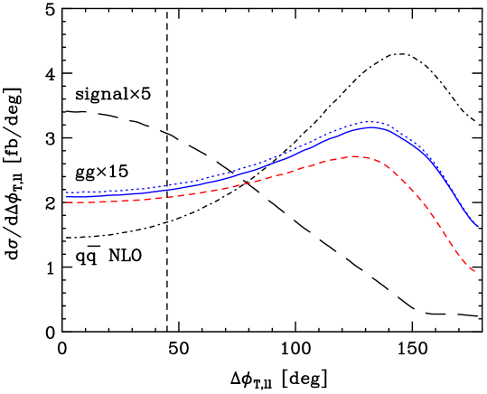
Figure 2: Distribution in the transverse-plane opening angle of the charged leptons $\Delta\phi_{T,\ell\ell}$ for $pp\to W^{\ast}W^{\ast}\to\ell\bar{\nu}\bar{\ell^{\prime}}\nu^{\prime}$ at the LHC. Displayed is the background process from gluon scattering without (dashed) and with the top-bottom loop (solid) – the latter also without off-shell $W$ effects (dotted) – each multiplied with a factor 15; the background from quark scattering at NLO (dot-dashed); and the signal process for $M_{H}=170$ GeV (long-dashed) multiplied with a factor 5. Input parameters as defined in the main text. Standard LHC cuts have been applied. The Higgs search cuts select the region $\Delta\phi_{T,\ell\ell}<45^{\circ}$ left of the vertical dashed line.

	$\sigma(pp\to W^{\ast}W^{\ast}\to\ell\bar{\nu}\bar{\ell^{\prime}}\nu^{\prime})$ [fb],  LHC
	quark loop	quark loop		interference
	generations 1,2	generation 3	$\frac{\displaystyle\rm gen.\,1,2,3}{\displaystyle\rm gens.\,1,2}$	$\frac{\rm gens.\,1,2,3}{\rm[gens.\,1,2]+[gen.\,3]}$
$\sigma_{tot}[gg]$	53.64(1)	2.859(3)	1.12	1.06
$\sigma_{bkg}[gg]$	1.3837(3)	0.00377(2)	1.02	1.02

Table 2: Cross sections for the gluon scattering contribution to $pp\to W^{\ast}W^{\ast}\to\ell\bar{\nu}\bar{\ell^{\prime}}\nu^{\prime}$ at the LHC ($\sqrt{s}=14$ TeV) without selection cuts ($tot$) and Higgs search selection cuts ($bkg$) applied. We show the cross section with 2 massless generations [20], the contribution of the top-bottom loop, and the size of the interference effects. The Higgs signal has not been included. The integration error is given in brackets.

An interesting distribution, which we did not display in Ref. [20] is the transverse mass distribution $\mbox{d}\sigma/\mbox{d}M_{T}$, where one uses a measurable proxy for the Higgs transverse mass defined by $M_{T}=\sqrt{(E_{T,\ell\ell}+E\hskip-7.95831pt\hbox to7.95831pt{\hss$/$\hss}_{T})^{2}-({\vec{p}}_{T,\ell\ell}+\vec{p}\hskip-6.5382pt\hbox to6.5382pt{\hss$/$\hss}_{T})^{2}}$, with $E_{T,\ell\ell}=\sqrt{p_{T,\ell\ell}^{2}+m_{\ell\ell}^{2}}$ and $E\hskip-7.95831pt\hbox to7.95831pt{\hss$/$\hss}_{T}=\sqrt{p\hskip-5.03125pt\hbox to5.03125pt{\hss$/$\hss}_{T}^{2}+m_{\ell\ell}^{2}}$ [50]. Cuts on the transverse mass $M_{T}$ provide an additional handle to suppress the background with respect to the Higgs signal, see e.g. Refs. [15, 45, 46]. In Fig. 3 we compare the $M_{T}$-distribution of the $q\bar{q}$ background in LO and NLO with the contribution from gluon-gluon scattering before and after applying Higgs search cuts. The figures reveal that the gluon-induced contribution becomes the dominant higher-order correction to the background process after Higgs selection cuts have been imposed.

Figure 3: Distribution in the transverse mass $M_{T}$ (as defined in the text) with standard cuts (left figure) and Higgs search cuts (right figure). Displayed are the total background from quark scattering at NLO and gluon-fusion (solid), and from quark scattering alone at LO (dotted) and NLO (dot-dashed).

We now turn to the discussion of the interference effects between the gluon-gluon induced signal and background processes. Table 3 shows cross sections for the signal and gluon-fusion background with and without interference. We show results for $M_{H}=140$, 170 and 200 GeV, spanning the Higgs mass range for which the $H\to WW$ decay mode is of particular relevance. It turns out that the interference effects are quite small and never exceed 10% of the gluon-induced signal plus background cross section. Adding the NLO background contribution from quark scattering, the overall effect of the interference term is always less than 5%. These results are consistent with the small signal-background interference observed in $pp\to H\to\gamma\gamma$ [51, 52]. Due to the imposed jet veto, we expect only small effects at the LHC when NLO corrections are taken into account for the signal [53] and $gg$ background.

	$\sigma[gg(\to H)\to W^{\ast}W^{\ast}\to\ell\bar{\nu}\bar{\ell^{\prime}}\nu^{\prime}]\ \ {\rm[fb]}$
cut selection	$tot$			$bkg$
$M_{H}{\rm[GeV]}$	$140$	$170$	$200$	$140$	$170$	$200$
$\sigma[{\rm signal}]$	79.83(2)	116.23(3)	75.40(2)	1.8852(5)	12.974(2)	1.6663(7)
$\sigma[{\rm signal+bkg(gg)}]$	132.50(5)	174.58(9)	134.46(5)	3.174(2)	15.287(6)	3.413(2)
$\frac{\sigma[{\rm sig+bkg(gg)}]}{\sigma[{\rm signal}]+\sigma[{\rm bkg(gg)}]}$	$0.948$	$0.991$	$0.993$	$0.962$	$1.062$	$1.108$

Table 3: Interference effects between the signal and gluon-induced background processes. Details as in Table 1.

In Fig. 4 we finally show the $W^{-}$ invariant-mass distribution without applying selection cuts for $M_{H}=140~{}{\rm GeV}\!<2M_{W}$. Although this distribution is not measurable it is instructive in understanding interference and off-shell effects. We compare the signal and the gluon-induced background with and without interference effects. In addition to a pronounced, narrow resonance at $M_{W}$, the $W^{-}$ invariant mass distribution exhibits a second small and broad resonance at about 55 GeV, which stems from the kinematic constraint imposed by the dominant Higgs resonance in the signal process. We note that without any selection cuts and for Higgs masses around 140 GeV, the gluon-induced background exceeds the Higgs-boson signal in the resonant region near $M_{W}$.

Figure 4: Distribution in the $W^{-}$ invariant mass for $M_{H}$ = 140 GeV. The resonant region is magnified on the right hand side. Complete $gg$ background without signal (dashed, blue), signal only (dotted), signal and background with interference (solid) and signal and background without interference (dot-dashed) are displayed. No selection cuts are applied ($tot$).

4 Conclusions

We have presented the first complete calculation of the loop-induced gluon-fusion process $gg\to W^{\ast}W^{\ast}\to\ell\bar{\nu}\bar{\ell^{\prime}}\nu^{\prime}$, including intermediate light and heavy quarks, and studied its importance for Higgs boson searches in the $H\to WW$ channel. We find that the top-bottom loop, which had been neglected in Ref. [20] contributes at a level of about 10-15% to the inclusive gluon-induced cross section but is strongly suppressed after Higgs search cuts have been imposed. We have also studied interference effects between signal and background processes and found them to be small (about 5% or less) in the relevant Higgs mass range between $M_{H}=140-200$ GeV. We provide the GG2WW package [40], a public parton-level Monte Carlo program and event generator for the process $gg\to W^{\ast}W^{\ast}\to\ell\bar{\nu}\bar{\ell^{\prime}}\nu^{\prime}$ that can be used to calculate cross sections with any set of cuts or any kind of differential distribution, or to generate weighted or unweighted events for experimental analyses.

Appendix A Auxilliary vector relations

$$p_{3}=\frac{t-s_{3}}{s}p_{1}+\frac{u-s_{3}}{s}p_{2}+\tilde{p}_{3}$$

$$p_{4}=\frac{u-s_{4}}{s}p_{1}+\frac{t-s_{4}}{s}p_{2}-\tilde{p}_{3}\,$$

$$p_{1}\cdot\tilde{p}_{3}=p_{2}\cdot\tilde{p}_{3}=0$$

$$k_{0}^{\mu}=\epsilon(p_{1},p_{2},\tilde{p}_{3},\mu)$$

$$\tilde{p}_{3}^{2}=-\frac{\det G}{2\;s^{2}}$$

To define the basis used in Eq. (6) we exploit that

$$p_{3}\cdot J_{3} = \frac{t-s_{3}}{s}p_{1}\cdot J_{3}+\frac{u-s_{3}}{s}p_{2}\cdot J_{3}+\tilde{p}_{3}\cdot J_{3}=0\ ,$$

$$p_{4}\cdot J_{4} = \frac{u-s_{4}}{s}p_{1}\cdot J_{4}+\frac{t-s_{4}}{s}p_{2}\cdot J_{4}-\tilde{p}_{3}\cdot J_{4}=0\ ,$$

$$J_{3}\cdot J_{4} = \frac{2}{s}(p_{1}\cdot J_{3}\;p_{2}\cdot J_{4}+p_{2}\cdot J_{3}\;p_{1}\cdot J_{4})-\frac{s}{ut-s_{3}s_{4}}\tilde{p}_{3}\cdot J_{3}\tilde{p}_{3}\cdot J_{4}$$

$$+\frac{4}{s(ut-s_{3}s_{4})}\epsilon(p_{1},p_{2},\tilde{p}_{3},J_{3})\,\epsilon(p_{1},p_{2},\tilde{p}_{3},J_{4})\ ,$$

$$\epsilon(p_{1},p_{2},J_{3},J_{4}) = -\frac{s}{ut-s_{3}s_{4}}[\tilde{p}_{3}\cdot J_{3}k_{0}\cdot J_{4}-\tilde{p}_{3}\cdot J_{4}k_{0}\cdot J_{3}]\ .$$

Appendix B Dimension splitting formulae

When using dimensional regularization in combination with genuinely 4-dimensional objects, one is forced to apply a calculational scheme to deal with the $\gamma_{5}$ problem. We apply standard dimension splitting rules [28] and use an $n$-dimensional loop momentum $k$ and gamma matrices $\gamma_{\mu}$, but work with 4-dimensional external momenta. The following rules are sufficient to evaluate the diagrams in Fig. 1:

$$k=\hat{k}+\tilde{k}\quad,\qquad k^{2}=\hat{k}^{2}+\tilde{k}^{2}\quad,$$

$$\gamma=\hat{\gamma}+\tilde{\gamma}\quad,\qquad\{\hat{\gamma}^{\mu},\tilde{\gamma}^{\nu}\}=0\quad,\qquad\{\hat{\gamma}^{\mu},\hat{\gamma}^{\nu}\}=\hat{g}^{\mu\nu}\quad,\qquad$$

$$p_{j}^{\mu}\gamma_{\mu}=p_{j}^{\mu}\hat{\gamma}_{\mu}\quad,\qquad p_{j}\cdot k=p_{j}\cdot\hat{k}\quad,$$

$$\{\hat{\gamma}^{\mu},\gamma_{5}\}=0\quad,\qquad[\tilde{\gamma}^{\mu},\gamma_{5}]=0\,.$$

All hat objects are defined in 4 dimensions, whereas the ones with tildes are $(n-4)$-dimensional remnants. Remaining integrals that contain remnants of the $n$-dimensional algebra, i.e. factors of $(\tilde{k}\cdot\tilde{k})^{\alpha}$ are evaluated with the following relations [54]:

$$\int\frac{d^{n}k}{i\pi^{n/2}}\frac{(\tilde{k}\cdot\tilde{k})^{\alpha}}{(k^{2}-M^{2})^{N}} = (-1)^{\alpha}\frac{\Gamma(\alpha-\epsilon)}{\Gamma(1-\epsilon)}\frac{n-4}{2}\;I_{N}^{n+2\alpha}\ ,$$

$$\int\frac{d^{n}k}{i\pi^{n/2}}\frac{(\tilde{k}\cdot\tilde{k})^{\alpha}k^{\mu}k^{\nu}}{(k^{2}-M^{2})^{N}} = (-1)^{\alpha+1}\frac{\Gamma(\alpha-\epsilon)}{\Gamma(1-\epsilon)}g^{\mu\nu}\frac{n-4}{4}\frac{n+2\alpha}{n}\,I_{N}^{n+2+2\alpha}\,.$$

The $n$-dimensional $N$-point integral is defined by [27]

$$I_{N}^{n} = \int\frac{d^{n}k}{i\pi^{n/2}}\frac{1}{\prod_{j=1}^{N}((k-r_{j})^{2}-m_{j}^{2})}$$

$$= (-1)^{N}\Gamma(N-n/2)\int\limits_{0}^{1}dx_{1}\dots dx_{N}\delta(1-\sum\limits_{l=1}^{N}x_{l})(M^{2})^{n/2-N}\,,$$

with $r_{j}=p_{1}+\dots+p_{j}$ and

$$M^{2} = \frac{1}{2}\sum\limits_{i,j=1}^{N}x_{i}S_{ij}x_{j}\;,\;S_{ij}=-(r_{i}-r_{j})^{2}+m_{i}^{2}+m_{j}^{2}\,.$$

Below we list all required integrals, expanded to the relevant order in $\epsilon$.

$$I_{4,\alpha=1}^{n,\mu\nu} = \int\frac{d^{n}k}{i\pi^{n/2}}\frac{\tilde{k}\cdot\tilde{k}\,k^{\mu}k^{\nu}}{\prod_{j=1}^{4}((k-r_{j})^{2}-m_{j}^{2})}=-\frac{g^{\mu\nu}}{8}+{\cal O}(\epsilon)$$

$$I_{4,\alpha=2}^{n} = \int\frac{d^{n}k}{i\pi^{n/2}}\frac{(\tilde{k}\cdot\tilde{k})^{2}}{\prod_{j=1}^{4}((k-r_{j})^{2}-m_{j}^{2})}=-\frac{1}{6}+{\cal O}(\epsilon)$$

$$I_{4}^{n,\alpha=1} = {\cal O}(\epsilon)$$

$$I_{3,\alpha=1}^{n} = \int\frac{d^{n}k}{i\pi^{n/2}}\frac{\tilde{k}\cdot\tilde{k}}{\prod_{j=1}^{3}((k-r_{j})^{2}-m_{j}^{2})}=-\frac{1}{2}+{\cal O}(\epsilon)\,$$

References

• [1] S. Haywood et al., “Electroweak physics,” arXiv:hep-ph/0003275, published in the proceedings of the “CERN Workshop on Standard Model Physics (and more) at the LHC”, 14-15 October 1999, Geneva, Switzerland. Editors G. Altarelli and M.L. Mangano, Geneva, CERN, 2000.
• [2] J. Ohnemus, Phys. Rev. D 44 (1991) 1403.
• [3] S. Frixione, Nucl. Phys. B 410 (1993) 280.
• [4] J. Ohnemus, Phys. Rev. D 50 (1994) 1931 [arXiv:hep-ph/9403331].
• [5] L. J. Dixon, Z. Kunszt and A. Signer, Nucl. Phys. B 531 (1998) 3 [arXiv:hep-ph/9803250].
• [6] L. J. Dixon, Z. Kunszt and A. Signer, Phys. Rev. D 60 (1999) 114037 [arXiv:hep-ph/9907305].
• [7] J. M. Campbell and R. K. Ellis, Phys. Rev. D 60 (1999) 113006 [arXiv:hep-ph/9905386].
• [8] S. Frixione and B. R. Webber, arXiv:hep-ph/0601192.
• [9] M. Grazzini, JHEP 0601, 095 (2006) [arXiv:hep-ph/0510337].
• [10] E. Accomando, A. Denner and A. Kaiser, Nucl. Phys. B 706 (2005) 325 [arXiv:hep-ph/0409247].
• [11] M. Dittmar and H. K. Dreiner, Phys. Rev. D 55 (1997) 167 [arXiv:hep-ph/9608317].
• [12] M. Dittmar and H. K. Dreiner, “$h_{0}\to W^{+}W^{-}\to l^{+}l^{\prime-}\nu/l\bar{\nu}/l^{\prime}$ as the dominant SM Higgs search mode at the LHC for M($h_{0}$) = 155 GeV to 180 GeV,” arXiv:hep-ph/9703401, published in the proceedings of the Ringberg Workshop “The Higgs Puzzle - What can We Learn from LEP2, LHC, NLC, and FMC?”, 8-13 December 1996, Ringberg, Germany. Editor B.A. Kniehl, Singapore, World Scientific, 1997.
• [13] E. W. N. Glover and J. J. van der Bij, Phys. Lett. B 219 (1989) 488.
• [14] C. Kao and D. A. Dicus, Phys. Rev. D 43 (1991) 1555.
• [15] M. Dührssen, K. Jakobs, J. J. van der Bij and P. Marquard, JHEP 0505 (2005) 064 [arXiv:hep-ph/0504006].
• [16] K. L. Adamson, D. de Florian and A. Signer, Phys. Rev. D 65 (2002) 094041 [arXiv:hep-ph/0202132].
• [17] K. L. Adamson, D. de Florian and A. Signer, Phys. Rev. D 67 (2003) 034016 [arXiv:hep-ph/0211295].
• [18] T. Matsuura and J. J. van der Bij, Z. Phys. C 51 (1991) 259.
• [19] C. Zecher, T. Matsuura and J. J. van der Bij, Z. Phys. C 64 (1994) 219 [arXiv:hep-ph/9404295].
• [20] T. Binoth, M. Ciccolini, N. Kauer and M. Krämer, JHEP 0503 (2005) 065 [arXiv:hep-ph/0503094].
• [21] T. Binoth, M. Ciccolini, N. Kauer and M. Krämer, in “Les Houches physics at TeV colliders 2005, standard model, QCD, EW, and Higgs working group: Summary report,” arXiv:hep-ph/0604120.
• [22] Z. Xu, D. Zhang, L. Chang, Nucl. Phys. B291 (1987) 392.
• [23] G. ’t Hooft and M. J. G. Veltman, Nucl. Phys. B 153 (1979) 365.
• [24] G. Passarino and M. J. G. Veltman, Nucl. Phys. B 160 (1979) 151.
• [25] T. Binoth, J. P. Guillet, G. Heinrich, E. Pilon and C. Schubert, JHEP 0510 (2005) 015 [arXiv:hep-ph/0504267].
• [26] T. Binoth, M. Ciccolini and G. Heinrich, arXiv:hep-ph/0601254.
• [27] T. Binoth, J. P. Guillet and G. Heinrich, Nucl. Phys. B 572 (2000) 361 [arXiv:hep-ph/9911342].
• [28] M. J. G. Veltman, Nucl. Phys. B 319 (1989) 253.
• [29] J. A. M. Vermaseren, arXiv:math-ph/0010025 (unpublished).
• [30] T. Hahn, Comput. Phys. Commun. 140 (2001) 418 [hep-ph/0012260].
• [31] T. Hahn and M. Perez-Victoria, Comput. Phys. Commun.  118 (1999) 153 [arXiv:hep-ph/9807565].
• [32] E. Boos et al., in proceedings of Workshop Physics at TeV Colliders, Les Houches, France, 21 May - 1 June 2001, arXiv:hep-ph/0109068.
• [33] F. A. Berends, R. Pittau and R. Kleiss, Nucl. Phys. B 424 (1994) 308 [arXiv:hep-ph/9404313].
• [34] R. Kleiss and R. Pittau, Comput. Phys. Commun.  83 (1994) 141 [arXiv:hep-ph/9405257].
• [35] N. Kauer and D. Zeppenfeld, Phys. Rev. D 65 (2002) 014021 [arXiv:hep-ph/0107181].
• [36] N. Kauer, Phys. Rev. D 67 (2003) 054013 [arXiv:hep-ph/0212091].
• [37] G. P. Lepage, J. Comput. Phys. 27 (1978) 192; G. P. Lepage, preprint CLNS-80/447, (1980).
• [38] http://hepsource.sf.net/OmniComp/
• [39] http://hepforge.cedar.ac.uk/lhapdf/
• [40] http://hepsource.sf.net/GG2WW/
• [41] C. Buttar et al., “Les Houches physics at TeV colliders 2005, standard model, QCD, EW, and Higgs working group: Summary report,” arXiv:hep-ph/0604120.
• [42] V. Drollinger, T. Binoth, M. Ciccolini, M. Dührssen and N. Kauer, “Modeling the production of W pairs at the LHC,” CERN-CMS-NOTE-2005-024.
• [43] CMS Physics, Technical Design Report, CERN/LHCC 2006-021.
• [44] M. Dittmar and H. K. Dreiner, CMS-NOTE-1997-083 (unpublished).
• [45] K. Jakobs, T. Trefzger, ALTLAS-PHYS-2000-015 (unpublished).
• [46] D. Green, K. Maeshima, J. Marraffino, R. Vidal, J. Womersley, W. Wu and S. Kunori, J. Phys. G 26 (2000) 1751.
• [47] G. Davatz, G. Dissertori, M. Dittmar, M. Grazzini and F. Pauss, JHEP 0405 (2004) 009 [arXiv:hep-ph/0402218].
• [48] A. Djouadi, J. Kalinowski and M. Spira, Comput. Phys. Commun.  108 (1998) 56 [arXiv:hep-ph/9704448].
• [49] J. Pumplin, D. R. Stump, J. Huston, H. L. Lai, P. Nadolsky and W. K. Tung, JHEP 0207 (2002) 012 [arXiv:hep-ph/0201195].
• [50] D. L. Rainwater and D. Zeppenfeld, Phys. Rev. D 60 (1999) 113004 [Erratum-ibid. D 61 (2000) 099901] [arXiv:hep-ph/9906218].
• [51] D. A. Dicus and S. S. D. Willenbrock, Phys. Rev. D 37 (1988) 1801.
• [52] L. J. Dixon and M. S. Siu, Phys. Rev. Lett.  90 (2003) 252001 [arXiv:hep-ph/0302233].
• [53] S. Catani, D. de Florian and M. Grazzini, JHEP 0201 (2002) 015 [arXiv:hep-ph/0111164].
• [54] T. Binoth, J. P. Guillet and G. Heinrich, arXiv:hep-ph/0609054.