On Effective Charges, Event Shapes and the size of Power Corrections

Abstract

We introduce and motivate the method of effective charges, and consider how to implement an all-orders resummation of large kinematical logarithms in this formalism. Fits for QCD $\Lambda$ and power corrections are performed for the ${e}^{+}{e}^{-}$ event shape obesrvables 1-thrust and heavy-jet mass, and somewhat smaller power corrections found than in the usual approach employing the “physical scale” choice.

I Introduction

In this talk I will describe some recent work together with Michael Dinsdale concerning the relative size of non-perturbative power corrections for QCD event shape observables r1 ; r1b . For ${e}^{+}{e}^{-}$ event shape means the DELPHI collaboration have found in a recent analysis that, if the next-to-leading order (NLO) perturbative corrections are evaluated using the method of effective charges r2 , then one can obtain excellent fits to data without includingany power corrections r3 ; r3b . In contrast fits based on the use of standard fixed-order perturbation theory in the $\overline{MS}$ scheme with a physical choice of renormalization scale equal to the c.m. energy, require additional power corrections ${C}_{1}/Q$ with ${C}_{1}\sim 1\;\rm{GeV}$. Power corrections of this size are also predicted in a model based on an infrared finite coupling r4 , which is able to fit the data reasonably well in terms of a single parameter. Given the DELPHI result it is interesting to consider how to extend the method of effective charges to event shape distributions rather than means.

II The method of effective charges

Consider an ${e}^{+}{e}^{-}$ observable ${\cal{R}}(Q)$, e.g. an event shape observable- thrust or heavy-jet mass, $Q$ being the c.m. energy.

$${\cal{R}}(Q)=a(\mu,{\rm{RS}})+\sum_{n>0}r_{n}(\mu/Q,{\rm{RS}})a^{n+1}(\mu,{\rm{RS}}).$$ (1)

Here $a\equiv{\alpha}_{s}/\pi$. Normalised with the leading coefficient unity, such an observable is called an effective charge. The couplant $a(\mu,{\rm{RS}})$ satisfies the beta-function equation

$$\frac{da(\mu,{\rm{RS}})}{d\ln(\mu)}=\beta(a)=-ba^{2}(1+ca+c_{2}a^{2}+c_{3}a^{3}+\cdots)\;.$$ (2)

Here $b=(33-2{N}_{f})/6$ and $c=(153-19{N}_{f})/12b$ are universal, the higher coefficients ${c}_{i}$, $i\geq{2}$, are RS-dependent and may be used to label the scheme, together with dimensional transmutation parameter $\Lambda$ r5 . The effective charge ${\cal{R}}$ satisfies the equation

$$\frac{d{\cal{R}}(Q)}{d\ln(Q)}=\rho({\cal{R}}(Q))=-b{\cal{R}}^{2}(1+c{\cal{R}}+\rho_{2}{\cal{R}}^{2}+\rho_{3}{\cal{R}}^{3}+\cdots)\;.$$ (3)

This corresponds to the beta-function equation in an RS where the higher-order corrections vanish and ${\cal{R}}=a$, the beta-function coefficients in this scheme are the RS-invariant combinations

$$\rho_{2} = c_{2}+r_{2}-r_{1}c-r_{1}^{2}$$

$$\rho_{3} = c_{3}+2r_{3}-4r_{1}r_{2}-2r_{1}\rho_{2}-r_{1}^{2}c+2r_{1}^{3}.$$ (4)

Eq.(3) for $d{\cal{R}}/d{\ln{Q}}$ can be integrated to give

$$b\ln\frac{Q}{{\Lambda}_{\cal{R}}}=\frac{1}{{\cal{R}}}+c{\ln}\left[\frac{c{\cal{R}}}{1+c{\cal{R}}}\right]+\int_{0}^{{\cal{R}}(Q)}{dx}\left[\frac{b}{\rho(x)}+\frac{1}{{x}^{2}(1+cx)}\right]\;.$$ (5)

The dimensionful constant ${\Lambda}_{\cal{R}}$ arises as a constant of integration. It is related to the dimensional transmutation parameter ${\tilde{\Lambda}}_{\overline{MS}}$ by the exact relation,

$${\Lambda}_{\cal{R}}={e}^{r/b}{\tilde{\Lambda}}_{\overline{MS}}\;.$$ (6)

Here ${r}\equiv{r}_{1}(1,\overline{MS})$ with $\mu=Q$, is the NLO perturbative coefficient. Eq.(5) can be recast in the form

$${\Lambda}_{\overline{MS}}=Q{\cal{F}}({\cal{R}}(Q)){\cal{G}}({\cal{R}}(Q)){e}^{-r/b}{(2c/b)}^{c/b}\;.$$ (7)

The final factor converts to the standard convention for $\Lambda$. Here ${\cal{F}}({\cal{R}})$ is the universal function

$${\cal{F}}({\cal{R}})={e}^{-1/b{\cal{R}}}{(1+1/c{\cal{R}})}^{c/b}\;,$$ (8)

and ${\cal{G}}({\cal{R}})$ is

$${\cal{G}}({\cal{R}})=1-\frac{{\rho}_{2}}{b}{\cal{R}}+O({\cal{R}}^{2})+{\ldots}\;.$$ (9)

Here ${\rho}_{2}$ is the NNLO ECH RS-invariant. If only a NLO calculation is available, as is the case for ${e}^{+}{e}^{-}$ jet observables, then ${\cal{G}}({\cal{R}})=1$, and

$${\Lambda}_{\overline{MS}}=Q{\cal{F}}({\cal{R}}(Q)){e}^{-r/b}{(2c/b)}^{c/b}\;.$$ (10)

Eq.(10) can be used to convert the measured data for the observable ${\cal{R}}$ into a value of ${\Lambda}_{\overline{MS}}$ bin-by-bin. Such an analysis was carried out in Ref. r6 for a number of ${e}^{+}{e}^{-}$ event shape observables, including thrust and heavy jet mass which we shall focus on here. It was found that the fitted $\Lambda$ values exhibited a clear plateau region, away from the two-jet region, and the region approaching $T=2/3$ where the NLO thrust distribution vanishes. The result for 1-thrust corrected for hadronization effects is shown in Fig. 1.

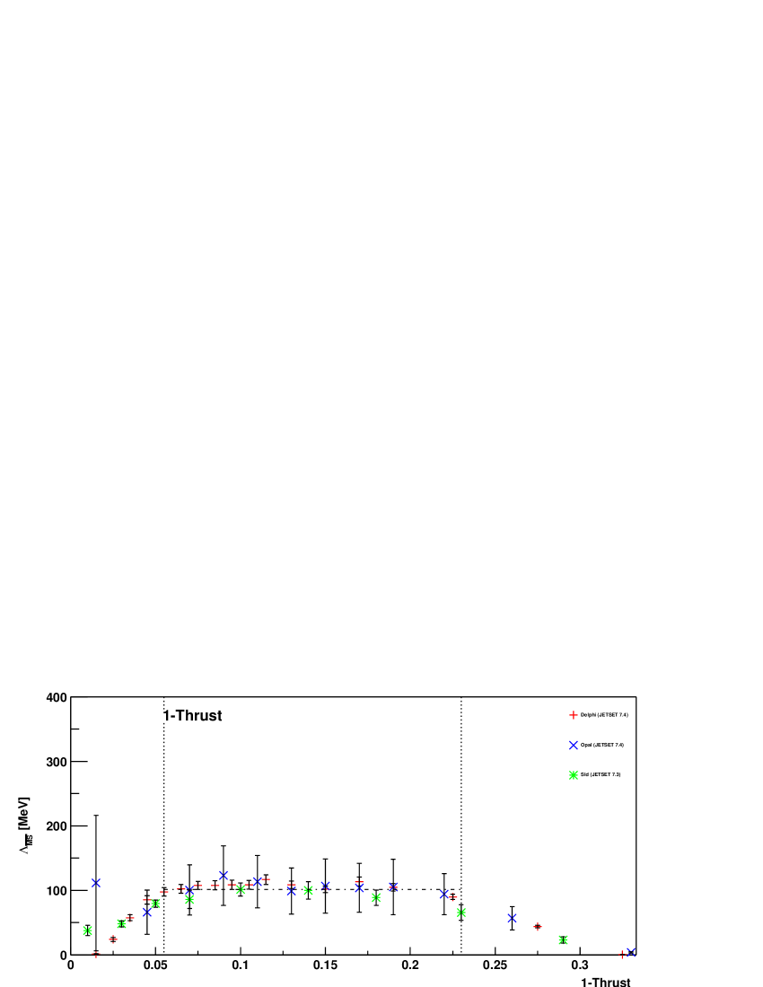
Figure 1: Values of ${\Lambda}_{\overline{MS}}$ obtained for hadronization corrected 1-thrust data. r6

Another way of motivating the effective charge approach is the idea of “complete renormalization group improvement” (CORGI) r6a . One can write the NLO coefficient ${r}_{1}(\mu)$ as

$${r_{1}}({\mu})=b{\ln}\frac{\mu}{{\tilde{\Lambda}}_{\overline{MS}}}-b{\ln}\frac{Q}{{\Lambda}_{\cal{R}}}\;.$$ (11)

Hence one can identify scale-dependent $\mu$-logs and RS-invariant “physical” UV $Q$-logs. Higher coefficients are polynomials in ${r}_{1}$.

$${r_{2}} = {r}_{1}^{2}+{r}_{1}c+({\rho}_{2}-{c_{2}})$$

$${r_{3}} = {r}_{1}^{3}+\frac{5}{2}c{r}_{1}^{2}+(3{\rho_{2}}-2{c_{2}}){r_{1}}+(\frac{{\rho}_{3}}{2}-\frac{c_{3}}{2})\;.$$ (12)

Given a NLO calculation of ${r}_{1}$, parts of ${r}_{2},{r_{3}},\ldots$ are “RG-predictable”. One usually chooses ${\mu}=xQ$ then $r_{1}$ is $Q$-independent, and so are all the $r_{n}$. The $Q$-dependence of ${\cal{R}}(Q)$ then comes entirely from the RS-dependent coupling $a(Q)$. However, if we insist that $\mu$ is held constant independent of $Q$ the only $Q$-dependence resides in the “physical” UV $Q$-logs in $r_{1}$. Asymptotic freedom then arises only if we resum these $Q$-logs to all-orders. Given only a NLO calculation, and assuming for simplicity that that we have a trivial one loop beta-function ${\beta}(a)=-b{a}^{2}$ so that $a(\mu)=1/b{\ln}(\mu/{\tilde{\Lambda}}_{\overline{MS}})$ the RG-predictable terms will be

$${\cal{R}}=a({\mu})\left(1+{\sum_{n>0}}{(a({\mu}){r}_{1}({\mu}))}^{n}\right)\;.$$ (13)

Summing the geometric progression one obtains

$${\cal{R}}(Q) = a({\mu})/\left[1-\left(b{\ln}\frac{{\mu}}{{\tilde{\Lambda}}_{\overline{MS}}}-b{\ln}\frac{Q}{{\Lambda}_{\cal{R}}}\right)a({\mu})\right]$$ (14)

$$= 1/b{\ln}(Q/{\Lambda}_{\cal{R}}).$$

The $\mu$-logs “eat themselves” and one arrives at the NLO ECH result ${\cal{R}}(Q)=1/b{\ln}(Q/{\Lambda}_{\cal{R}})$.

As we noted earlier, r3 ; r3b , use of NLO effective charge perturbation theory (Renormalization Group invariant (RGI) perturbation theory) leads to excellent fits for ${e}^{+}{e}^{-}$ event shape means consistent with zero power corrections, as illustrated in Figure 2. taken from Ref.r3 .

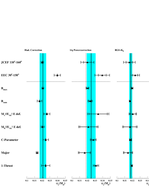
Figure 2: Fits for ${\alpha}_{s}(M_{Z})$ for means of ${e}^{+}{e}^{-}$ event shape observables taken from Ref.r3 . The quality of the “pure RGI” fits on the right is noteworthy.

Given this result it would seem worthwhile to extend the effective charge approach to event shape distributions. It is commonly stated that the method of effective charges is inapplicable to exclusive quantities which depend on multiple scales. However given an observable ${\cal{R}}({Q}_{1},{Q}_{2},{Q}_{3},\ldots,{Q}_{n})$ depending on $n$ scales it can always be written as

$${\cal{R}}={\cal{R}}({Q}_{1},{Q}_{2}/{Q}_{1},\ldots,{Q}_{n}/{Q}_{1}){\equiv}{\cal{R}}_{{x}_{2}{x}_{3}\ldots{x}_{n}}({Q}_{1})\;.$$ (15)

Here the ${x}_{i}{\equiv}{Q}_{i}/{Q}_{1}$ are dimensionless quantities that can be held fixed, allowing the ${Q}_{1}$ evolution of ${\cal{R}}$ to be obtained as before. In the 2-jet region for ${e}^{+}{e}^{-}$ observables large logarithms $L={\ln}(1/{x}_{i})$ arise and need to be resummed to all-orders.

III Resumming large logarithms for event shape distributions

Event shape distributions for thrust ($T$) or heavy-jet mass (${\rho}_{h}$) contain large kinematical logarithms, $L={\ln}(1/y)$, where $y=(1-T),\;{\rho}_{h},\cdots$.

$$\frac{1}{\sigma}\frac{d\sigma}{dy}=A_{LL}(aL^{2})+L^{-1}A_{NLL}(aL^{2})+\cdots\;.$$ (16)

Here $LL$, $NLL$, denote leading logarithms, next-to-leading logarithms, etc. For thrust and heavy-jet mass the distributions exponentiate r7

$$R_{y}(y^{\prime}) \equiv \int_{0}^{y^{\prime}}dy\frac{1}{\sigma}\frac{d\sigma}{dy}=C(a\pi)\exp(Lg_{1}(a\pi L)$$ (17)

$$+ g_{2}(a\pi L)+ag_{3}(a\pi L)+\cdots)+D(a\pi,y)\;.$$

Here $g_{1}$ contains the LL and $g_{2}$ the NLL. $C=1+O(a)$ is independent of $y$, and $D$ contains terms that vanish as $y\rightarrow{0}$. It is natural to define an effective charge ${\cal{R}}(y^{\prime})$ so that

$$R_{y}(y^{\prime})=\exp(r_{0}(y^{\prime}){\cal{R}}(y^{\prime}))\;.$$ (18)

This effective charge will have the expansion

$$r_{0}(L){\cal{R}}(L)=r_{0}(L)(a+r_{1}(L)a^{2}+r_{2}(L)a^{3}+\cdots)\;.$$ (19)

Here ${r}_{0}(L)\sim{L}^{2}$, and the higher coefficients ${r}_{n}(L)$ have the structure

$$r_{n}=r_{n}^{\rm LL}L^{n}+r_{n}^{\rm NLL}L^{n-1}+\cdots$$ (20)

Usually one resums these logarithms to all-orders using the known closed-form expressions for ${g}_{1}(aL)$ and ${g}_{2}(aL)$, where $a$ is taken to be the ${\overline{MS}}$ coupling with a “physical” scale choice $\mu=Q$ (${\overline{MS}}$PS). Instead we want to resum logarithms to all-orders in the ${\rho}({\cal{R}})$ function (ECH). The form of the ${\rho}_{n}$ RS-invariants (Eq.(4)) means that the ${\rho}_{n}$ have the structure

$$\rho_{n}=\rho_{n}^{\rm LL}L^{n}+\rho_{n}^{\rm NLL}L^{n-1}+\cdots\;.$$ (21)

One can then define all-orders RS-invariant $LL$ and $NLL$ approximations to ${\rho}({\cal{R}})$,

$$\rho_{\rm LL}({\cal{R}}) = -b{\cal{R}}^{2}(1+c{\cal{R}}+\sum_{n=2}^{\infty}\rho_{n}^{\rm LL}L^{n}{\cal{R}}^{n})$$

$$\rho_{\rm NLL}({\cal{R}}) = -b{\cal{R}}^{2}(1+c{\cal{R}}$$ (22)

$$+ \sum_{n=2}^{\infty}(\rho_{n}^{\rm LL}L^{n}+\rho_{n}^{\rm NLL}L^{n-1}){\cal{R}}^{n})\;.$$

The resummed ${\rho}_{\rm NLL}({\cal{R}})$ can then be used to solve for ${\cal{R}}_{\rm NLL}$ by inserting it in Eq.(5). Notice that since ${\Lambda}_{\cal{R}}$ involves the exact value of ${r}_{1}(1,\overline{MS})$ there is no matching problem as in the standard $\overline{MS}$PS approach. The resummed ${\rho}_{LL}({\cal{R}})$ can be straightforwardly numerically computed using

$${\rho}_{\rm LL}(x)=\beta(a)\frac{d\cal{R}_{\rm LL}}{da}=-ba^{2}\frac{d\cal{R}_{\rm LL}}{da}\;,$$ (23)

with $a$ chosen so that ${\cal{R}}_{\rm LL}(a)=x$. The same relation with ${\beta}(a)=-b{a}^{2}(1+ca)$ suffices for ${\rho}_{NLL}({\cal{R}})$, although in this case one needs to remove $NNLL$ terms, e.g. an ${L}^{0}$ term which would otherwise be included in ${\rho}_{2}$. This can be accomplished by numerically taking limits ${L}\rightarrow{\infty}$ with ${L}{\cal{R}}$ fixed.

As we have noted a crucial feature of the effective charge approach is that it resums to all-orders RG-Predictable pieces of the higher-order coefficients, thus the NLO ECH result (assuming $c=0$ for simplicity) corresponds to an RS-invariant resummation (c.f. Eq.(13).)

$$a+{r}_{1}{a}^{2}+{r}_{1}^{2}{a}^{3}+\cdots+{r}_{1}^{n}{a}^{n+1}+\cdots\;.$$ (24)

Thus even at fixed-order without any resummation of large logs in ${\rho}({\cal{R}})$ a partial resummation of large logs is automatically performed. Furthermore one might expect that the LL ECH result contains already NLL pieces of the standard ${\overline{MS}}$PS result.

Figure 3: Comparison of the 1-thrust distribution using various NLO approximations in the 2-jet region. The solid curve arises from exponentiating the NLO ECH. The dashed curve is obtained by expanding this to NLO in ${\overline{MS}}$PS. The dotted curve is an unexponentiated NLO ECH fit. DELPHI data at $Q={M}_{Z}$ are plotted. ${\Lambda}_{\overline{MS}}=212\;\rm{MeV}$ is assumed.

Figure 4: For 1-thrust the ratio of the NLL ${\overline{MS}}$PS coefficient at O(${a}^{n}$) “predicted” from the LL ECH result to the exact result (diamonds). The triangles show the “prediction” from the NLO ECH result.

In Figure 3 we show various NLO approximations. Notice that the solid curve, which corresponds to the exponentiated NLO ECH result, is a surprisingly good fit even in the 2-jet region, whereas the dashed curve which is the NLO $\overline{MS}$PS result, has a badly misplaced peak. The all-orders partial resummation of large logs in Eq.(15) gives a reasonable 2-jet peak. Figure 4 shows that the NLL ${\overline{MS}}$PS coefficients “predicted” from the LL ECH result by re-expanding it in the $\overline{MS}$PS coupling are in good agreement with the exact coeffiecients out to O(${a}^{10}$).

IV Fits for ${\Lambda}_{\overline{MS}}$ and power corrections

We now turn to fits simultaneously extracting ${\Lambda}_{\overline{MS}}$ and the size of power corrections ${C}_{1}/Q$ from the data. To facilitate this we use the result that inclusion of power corrections effectively shifts the event shape distributions, which can be motivated by considering simple models of hadronization, or through a renormalon analysis r8 . Thus we define

$${R}_{PC}(y)={R}_{PT}(y-{C}_{1}/Q)\;.$$ (25)

This shifted result is then fitted to the data for 1-thrust and heavy jet mass. ${e}^{+}{e}^{-}$ data spanning the c.m. energy range from $44-189$ GeV was used (see r1 for the complete list of references). The resulting fits for 1-thrust and heavy-jet mass are shown in Figures 5. and 6..

The ECH fits for thrust and heavy jet mass show great stability going from NLO to LL to NLL, presumably because at each stage a partial resummation of higher logs is automatically performed. The power corrections required with ECH are somewhat smaller than those found with ${\overline{MS}}$PS, but we do not find as dramatic a reduction as DELPHI find for the means. This may be because their analysis corrects the data for bottom quark mass effects which we have ignored. The fitted value of ${\Lambda}_{\overline{MS}}$ for ECH is much smaller than that found with ${\overline{MS}}$PS, (${\alpha}_{s}(M_{Z})=0.106$ (thrust) and $0.109$ (heavy-jet mass)). Similarly small values are found with the Dressed Gluon Exponentiation (DGE) approach r9 . A problem with the effective charge resummations is that the ${\rho}({\cal{R}})$ function contains a branch cut which limits how far into the 2-jet region one can go. We are limited to $1-T>0.05{M}_{Z}/Q$ in the fits we have performed. This branch cut mirrors a corresponding branch cut in the resummed $g_{1}(aL)$ function. Similarly as $1-T$ approaches $1/3$ the leading coefficient ${r}_{0}(L)$ vanishes and the Effective Charge formalism breaks down. We need to restrict the fits to $1-T<0.18$. From the “RG-predictability” arguments we might expect that these difficulties would also become apparent for a NNLL ${\overline{MS}}$PS resummation. One will be able to check this expectation when a result for ${g}_{3}(a\pi L)$ becomes available.

Figure 5: Fits to 1-thrust for ${\Lambda}_{\overline{MS}}$ and $C_{1}$. Solid $2\sigma$ error ellipses are for ECH, dashed are ${\overline{MS}}$PS. The arrows show the effect of varying the scale between $Q/2<\mu<2Q$.

Figure 6: Fits for heavy-jet mass.

V Extension to event shape means at HERA

Event shape means have also been studied in DIS at HERA r10 . For such processes one has a convolution of proton pdf’s and hard scattering cross-sections,

$$\frac{d{\sigma}(ep\rightarrow X,Q)}{dX}=\sum_{a}\int{d\xi}{f}_{a}(\xi,M)\frac{d{\hat{\sigma}}(ea\rightarrow X,Q,M)}{dX}\;.$$ (26)

There is no way to directly relate such quantities to effective charges. The DIS cross-sections will depend on a factorization scale $M$, and a renormalization scale $\mu$ at NLO. In principle one could identify unphysical scheme-dependent ${\ln}(M/{\tilde{\Lambda}}_{\overline{MS}})$ and ${\ln}({\mu}/{\tilde{\Lambda}}_{\overline{MS}})$, and physical UV $Q$-logs, and then by all-orders resummation get the $M$ and $\mu$-dependence to “eat itself”. The pattern of logs is far more complicated than the geometrical progression in the effective charge case, and a CORGI result for DIS has not been derived so far. Instead one can use the Principle of Minimal Sensitivity (PMS) r5 , and for an event shape mean $\langle{y}\rangle$ look for a stationary saddle point in the $(\mu,M)$ plane r11 . It turns that there are large cancellations between the NLO corrections for quark and gluon initiated subprocesses. One can distinguish between two approaches, ${PMS}_{1}$ where one seeks a saddle point in the $(\mu,M)$ plane for the sum of parton subprocesses, and ${PMS}_{2}$ where one introduces two separate scales ${\mu}_{q}$ and ${\mu}_{g}$ and finds a saddle point in $({\mu}_{q},{\mu}_{g},M)$. ${PMS}_{1}$ gives power corrections fits comparable to ${\overline{MS}}$PS with $M={\mu}=Q$. ${PMS}_{2}$ in contrast gives substantially reduced power corrections. This is shown in Figure 7 for a selection of HERA event shape means. Given large cancellations of NLO corrections RG-improvement should be performed separately for the $q$ and $g$-initiated subprocesses, and so ${PMS}_{2}$ which indeed fits the data best, is to be preferred.

Figure 7: The dashed line corresponds to ${PMS}_{1}$, and the solid line to the physical scale choice $M=\mu=Q$. The dotted line is ${PMS}_{2}$ and is in much better agreement with the data points. r11

VI Conclusions

Event shape means in ${e}^{+}{e}^{-}$ annihilation are well-fitted by NLO perturbation theory in the effective charge approach, without any power corrections being required. With the usual ${\overline{MS}}$PS approach power corrections $C_{1}/Q$ are required with $C_{1}\sim{1}$ GeV. Similarly sized power corrections are predicted in the model of Ref.r4 . It would be interesting to modify this model so that its perturbative component matched the effective charge prediction, but this has not been done. We showed how resummation of large logarithms in the effective charge beta-function $\rho({\cal{R}})$ could be carried out for ${e}^{+}{e}^{-}$ event shape distrtibutions. If the distributions are represented by an exponentiated effective charge then even at NLO a partial resummation of large logarithms is performed. As shown in Figure 3 this results in good fits to the 1-thrust distribution, with the peak in the 2-jet region in rough agreement with the data. In contrast the ${\overline{MS}}$PS prediction has a badly misplaced peak in the 2-jet region, and is well below the data for the realistic value of ${\Lambda}_{\overline{MS}}=212$ MeV assumed. We further showed in Figure 4 that the LL ECH result contains already a large part of the NLL ${\overline{MS}}$PS result. We found unfortunately that $\rho({\cal{R}})$ contains a branch point mirroring that in the resummed ${g}_{1}(aL)$ function. This limited the fit range we could consider. We fitted for power corrections and ${\Lambda}_{\overline{MS}}$ to the 1-thrust distribution and heavy-jet mass distributions, finding somewhat reduced power corrections for the ECH fits compared to ${\overline{MS}}$PS, with good stability going from NLO to LL to NLL. The suggestion of the “RG-predictability” manifested in Figure 4 would be that the NLL ECH result contains a large part of the NNLL ${\overline{MS}}$PS result. This suggests that the branch point problem which limits the ability to describe the 2-jet peak, would also show up given a NNLL analysis. This can be checked once the ${g}_{3}(aL)$ function becomes available. Recent work on event shape means in DIS was briefly mentioned and seemed to indicate that greatly reduced power corrections are found when a correctly optimised PMS approach is used.

- (1) M.J. Dinsdale and C.J. Maxwell, Nucl. Phys. B713 (2005) 465.
- (2) C.J. Maxwell, talk delivered at the FRIF workshop on First Principles QCD of Hadron Jets. [hep-ph/0607039].
- (3) G. Grunberg, Phys. Lett. B95 (1980) 70; Phys. Rev. D29 (1984) 2315.
- (4) DELPHI Collaboration (J. Abdallah et. al.) Eur. Phys. J. C29 (2003) 285.
- (5) K. Hamacher, talk delivered at the FRIF Workshop on First Principles QCD of Hadron Jets. [hep-ex/0605123].
- (6) Y.L. Dokshitzer and B.R. Webber, Phys. Lett. B404 (1997) 321.
- (7) P.M. Stevenson, Phys. Rev. D23 (1981) 2916.
- (8) S.J. Burby and C.J. Maxwell, Nucl. Phys. B609 (2001) 193.
- (9) C.J. Maxwell [hep-ph/9908463]; C.J. Maxwell and A. Mirjalili, Nucl. Phys. B611, 423 (2001).
- (10) S. Catani, G. Turnock, B.R. Webber and L. Trentadue, Phys. Lett. B263 (1991) 491.
- (11) B.R. Webber [hep-ph/9411384].
- (12) E. Gardi and J. Rathsman, Nucl. Phys. B638 (2002) 243.
- (13) C. Adloff et al. [H1 Collaboration], Eur. Phys. J. C 14 (2000) 255 [Erratum-ibid. C 18 (2000) 417] [arXiv:hep-ex/9912052].
- (14) M.J. Dinsdale [arXiv:hep-ph/0512069].