NLO jet production at central rapidities in $k_{T}$ factorization

Abstract:

In this contribution we discuss the inclusive production of jets in central regions of rapidity in the context of $k_{T}$–factorization at next–to–leading order (NLO). We work in the Regge limit of QCD and use the NLO BFKL results. A jet cone definition is proposed together with a phase–space separation into multi–Regge and quasi–multi–Regge kinematics. We discuss scattering of highly virtual photons, with a symmetric energy scale to separate the impact factors from the gluon Green’s function, and hadron–hadron collisions, with a non–symmetric scale choice.

1 Introduction

The study of jet production in perturbative QCD is an important element of phenomenological studies at present and future colliders. At high energies the understanding of multijet events becomes mandatory. In collinear factorization the theoretical analysis of multijet production is complicated since there is a large number of contributing diagrams. However, if we focus on the Regge asymptotics (small–$x$ region) of scattering amplitudes then it is possible to describe the production of a large number of jets. The corresponding phase space is that where the center–of–mass energy, $s$, can be considered asymptotically larger than any of the other scales. In this region the dominating Feynman diagrams are those with gluons exchanged in the $t$–channel. To resum contributions of the form $\left(\alpha_{s}\ln{s}\right)^{n}$ to all orders, with $\alpha_{s}$ being the coupling constant, it is possible to use the Balitsky–Fadin–Kuraev–Lipatov (BFKL) framework [1].

The concept of a Reggeized gluon is fundamental in the construction of the BFKL approach. Colour octet exchange in Regge asymptotics can be described by a $t$–channel gluon with its propagator modified by a multiplicative factor depending on a power of $s$. This power corresponds to the gluon Regge trajectory which is a function of the transverse momenta and is divergent in the infrared. This divergence is removed when real emissions are included using gauge invariant Reggeon–Reggeon–gluon couplings. This allows us to describe scattering amplitudes with a large number of partons in the final state. The $\left(\alpha_{s}\ln{s}\right)^{n}$ terms correspond to the leading–order (LO) approximation and provide a simple picture of the underlying physics. This approximation has limitations: in leading order both $\alpha_{s}$ and the factor scaling the energy $s$ in the resummed logarithms, $s_{0}$, are free parameters not determined by the theory. These free parameters can be fixed if next–to–leading terms $\alpha_{s}\left(\alpha_{s}\ln{s}\right)^{n}$ are included [2]. At this improved accuracy, diagrams contributing to the running of the coupling have to be included, and also $s_{0}$ is not longer undetermined. The phenomenological importance of the NLO effects has been recently shown for azimuthal angle decorrelations in Mueller–Navelet jets in Ref. [3].

The LO Reggeon–Reggeon–gluon vertex corresponds to one gluon emission which can possibly generate a single jet. At NLO the emission vertex also contains Reggeon–Reggeon–gluon–gluon and Reggeon–Reggeon–quark–antiquark terms. In this contribution we are interested in the description of the inclusive production of a single jet in the NLO BFKL formalism. The relevant events will be those with only one jet produced in the central rapidity region of the detector. To find the probability of production of these events it is needed to introduce a jet definition in the emission vertex. This is simple at LO, but at NLO one should study the possibility of double emission in the same region of rapidity, which could lead to the production of one or two jets.

In the present text we highlight the main elements presented in the analysis of Ref. [4]. In that work we discuss in detail the correct treatment of the different scales present in the amplitudes paying particular attention to the separation of multi–Regge and quasi–multi–Regge kinematics. There we also discuss similarities and discrepancies with the earlier work of Ref. [5].

Our analysis is performed for two different cases: inclusive jet production in the scattering of two photons with large and similar virtualities, and in hadron–hadron collisions. In the former case the cross section has a factorized form in terms of photon impact factors and gluon Green’s function. In the latter, with a momentum scale for the hadron lower than the typical $k_{T}$ entering the production vertex, the gluon Green’s function needs a modified BFKL kernel which incorporates some $k_{T}$–evolution from the nonperturbative, and model dependent, proton impact factor to the perturbative jet production vertex.

For hadron–hadron scattering, our cross section formula contains an unintegrated gluon density which, in addition to the usual dependence on the longitudinal momentum fraction, typical of collinear factorization, carries an explicit dependence on the transverse momentum $k_{T}$. This scheme is known as $k_{T}$–factorization. In the small–$x$ region, where this type of factorization has attracted particular interest, the BFKL framework offers the possibility to formulate, in a systematic way, the generalization of the $k_{T}$–factorization to NLO. It is then possible to interpret our analysis as a contribution to the more general question of how to formulate the unintegrated gluon density and the $k_{T}$–factorization scheme at NLO: our results can be considered as the small–$x$ limit of a more general formulation.

2 Inclusive jet production at LO

To initiate the discussion we first study the interaction between two photons with large virtualities $Q_{1,2}^{2}$ in the Regge limit $s\gg|t|\sim Q_{1}^{2}\sim Q_{2}^{2}$. In this region the total cross section can be written as a convolution of the photon impact factors with the gluon Green’s function, i.e.

$$\sigma(s)=\int\frac{d^{2}{\bf k}_{a}}{2\pi{\bf k}_{a}^{2}}\int\frac{d^{2}{\bf k}_{b}}{2\pi{\bf k}_{b}^{2}}\,\Phi_{A}({\bf k}_{a})\,\Phi_{B}({\bf k}_{b})\,\int_{\delta-i\infty}^{\delta+i\infty}\frac{d\omega}{2\pi i}\left(\frac{s}{s_{0}}\right)^{\omega}f_{\omega}({\bf k}_{a},{\bf k}_{b}).$$ (1)

A convenient choice for the energy scale is $s_{0}=|{\bf k}_{a}|\,|{\bf k}_{b}|$ since this naturally introduces the rapidities $y_{\tilde{A}}$ and $y_{\tilde{B}}$ of the emitted particles with momenta $p_{\tilde{A}}$ and $p_{\tilde{B}}$ given that $\left(\frac{s}{s_{0}}\right)^{\omega}=e^{\omega(y_{\tilde{A}}-y_{\tilde{B}})}$.

The gluon Green’s function $f_{\omega}$ corresponds to the solution of the BFKL equation

$$\omega f_{\omega}({\bf k}_{a},{\bf k}_{b}) = \delta^{2}({\bf k}_{a}-{\bf k}_{b})+\int d^{2}{\bf k}\;\mathcal{K}({\bf k}_{a},{\bf k})f_{\omega}({\bf k},{\bf k}_{b}),$$ (2)

with kernel

$$\mathcal{K}({\bf k}_{a},{\bf k}) = 2\,\omega({\bf k}_{a}^{2})\,\delta^{2}({\bf k}_{a}-{\bf k})+\mathcal{K}_{r}({\bf k}_{a},{\bf k}),$$ (3)

where $\omega({\bf k}_{a}^{2})$ is the gluon Regge trajectory and $\mathcal{K}_{r}$ is the real emission contribution to the kernel which we discus in detail in the following.

It is possible to single out one gluon emission by extracting its emission probability from the BFKL kernel. By selecting one emission to be exclusive we factorize the gluon Green’s function into two components. Each of them connects one of the external particles to the jet vertex, and depends on the total energies of the subsystems $s_{AJ}=(p_{A}+q_{b})^{2}$ and $s_{BJ}=(p_{B}+q_{a})^{2}$, respectively. We have drawn a graph indicating this separation in Fig. 1. The symmetric situation suggests the choices $s_{0}^{(AJ)}=|{\bf k}_{a}|\,|{\bf k}_{J}|$ and $s_{0}^{(BJ)}=|{\bf k}_{J}|\,|{\bf k}_{b}|$, respectively, as the suitable energy scales for the subsystems. These choices can be related to the relative rapidity between the jet and the external particles. To set the ground for the NLO discussion of next section we introduce an additional integration over the rapidity $\eta$ of the central system in the form

$$\frac{d\sigma}{d^{2}{\bf k}_{J}dy_{J}}=\int d^{2}{\bf q}_{a}\int d^{2}{\bf q}_{b}\int d\eta\left[\int\frac{d^{2}{\bf k}_{a}}{2\pi{\bf k}_{a}^{2}}\,\Phi_{A}({\bf k}_{a})\,\int_{\delta-i\infty}^{\delta+i\infty}\frac{d\omega}{2\pi i}e^{\omega(y_{A}-\eta)}f_{\omega}({\bf k}_{a},{\bf q}_{a})\right]\\ \times\mathcal{V}({\bf q}_{a},{\bf q}_{b},\eta;{\bf k}_{J},y_{J})\;\times\left[\int\frac{d^{2}{\bf k}_{b}}{2\pi{\bf k}_{b}^{2}}\,\Phi_{B}({\bf k}_{b})\int_{\delta-i\infty}^{\delta+i\infty}\frac{d\omega^{\prime}}{2\pi i}e^{\omega^{\prime}(\eta-y_{B})}f_{\omega^{\prime}}(-{\bf q}_{b},-{\bf k}_{b})\right]$$ (4)

with the LO emission vertex being

$$\mathcal{V}({\bf q}_{a},{\bf q}_{b},\eta;{\bf k}_{J},y_{J})=\mathcal{K}_{r}^{\rm(Born)}\left({\bf q}_{a},-{\bf q}_{b}\right)\,\delta^{(2)}\left({\bf q}_{a}+{\bf q}_{b}-{\bf k}_{J}\right)\,\delta(\eta-y_{J}).$$ (5)

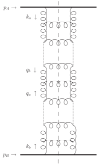
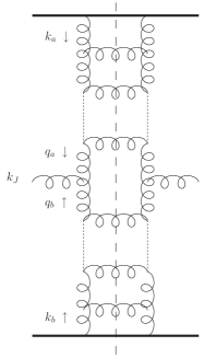
Figure 1: Total cross section and inclusive one jet production in the BFKL approach.

If the colliding external particles provide no perturbative scale, as it is the case in hadron–hadron collisions, then the jet is the only hard scale in the process and we have to deal with an asymmetric situation. In such a configuration the scales $s_{0}$ should be chosen as ${\bf k}_{J}^{2}$ alone. At LO accuracy $s_{0}$ is arbitrary and we are indeed free to make this choice. At this stage it is possible to introduce the concept of unintegrated gluon density in the hadron. This represents the probability of resolving a gluon carrying a longitudinal momentum fraction $x$ from the incoming hadron, and with a certain transverse momentum $k_{T}$. Its relation to the gluon Green’s function would be

$$g(x,{\bf k})=\int\frac{d^{2}{\bf q}}{2\pi{\bf q}^{2}}\,\Phi_{P}({\bf q})\,\int_{\delta-i\infty}^{\delta+i\infty}\frac{d\omega}{2\pi i}\,x^{-\omega}f_{\omega}({\bf q},{\bf k}).$$ (6)

With this new interpretation we can then rewrite Eq. (4) as

$$\frac{d\sigma}{d^{2}{\bf k}_{J}dy_{J}}=\int d^{2}{\bf q}_{a}\int dx_{1}\int d^{2}{\bf q}_{b}\int dx_{2}\;g(x_{1},{\bf q}_{a})g(x_{2},{\bf q}_{b})\mathcal{V}({\bf q}_{a},x_{1},{\bf q}_{b},x_{2};{\bf k}_{J},y_{J}),$$ (7)

with the LO jet vertex for the asymmetric situation being

$$\mathcal{V}({\bf q}_{a},x_{1},{\bf q}_{b},x_{2};{\bf k}_{J},y_{J})=\mathcal{K}_{r}^{\rm(Born)}\left({\bf q}_{a},-{\bf q}_{b}\right)\\ \times\delta^{(2)}\left({\bf q}_{a}+{\bf q}_{b}-{\bf k}_{J}\right)\,\delta\left(x_{1}-\sqrt{\frac{{\bf k}_{J}^{2}}{s}}e^{y_{J}}\right)\delta\left(x_{2}-\sqrt{\frac{{\bf k}_{J}^{2}}{s}}e^{-y_{J}}\right).$$ (8)

3 Inclusive jet production at NLO

A similar approach remains valid when jet production is considered at NLO. The crucial step in this direction is to modify the LO jet vertex of Eq. (5) and Eq. (8) to include new configurations present at NLO. We show how this is done in the following first subsection. In the second subsection we implement this vertex in a scattering process.

3.1 The NLO jet vertex

For those parts of the NLO kernel responsible for one gluon production we proceed in exactly the same way as at LO. The treatment of those terms related to two particle production is more complicated since for them it is necessary to introduce a jet algorithm. In general terms, if the two emissions generated by the kernel are nearby in phase space they will be considered as one single jet, otherwise one of them will be identified as the jet whereas the other will be absorbed as an untagged inclusive contribution. Hadronization effects in the final state are neglected and we simply define a cone of radius $R_{0}$ in the rapidity–azimuthal angle space such that two particles form a single jet if $R_{12}\equiv\sqrt{(\phi_{1}-\phi_{2})^{2}+(y_{1}-y_{2})^{2}}<R_{0}$. As long as only two emissions are involved this is equivalent to the $k_{T}$–clustering algorithm.

To introduce the jet definition in the $2\rightarrow 2$ components of the kernel it is convenient to combine the gluon and quark matrix elements together with the MRK contribution:

$$\left({\cal K}_{Q\bar{Q}}+{\cal K}_{GG}\right)({\bf q}_{a},-{\bf q}_{b})\equiv\int d^{D-2}{{\bf k}_{2}}\int dy_{2}\,\left|\mathcal{B}({\bf q}_{a},{\bf q}_{b},{\bf k}_{1},{\bf k}_{2})\right|^{2}$$

$$= \int d^{D-2}{{\bf k}_{2}}\int dy_{2}\,\Bigg{\{}\left|\mathcal{A}_{2q}({\bf q}_{a},{\bf q}_{b},{\bf k}_{1},{\bf k}_{2})\right|^{2}+\left|\mathcal{A}_{2g}({\bf q}_{a},{\bf q}_{b},{\bf k}_{1},{\bf k}_{2})\right|^{2}\theta(s_{\Lambda}-s_{12})$$

$$-{\cal K}^{\rm(Born)}({\bf q}_{a},{\bf q}_{a}-{\bf k}_{1})\,{\cal K}^{\rm(Born)}({\bf q}_{a}-{\bf k}_{1},-{\bf q}_{b})\;\frac{1}{2}\,\theta\left(\ln\frac{s_{\Lambda}}{{\bf k}_{2}^{2}}-y_{2}\right)\theta\left(y_{2}-\ln\frac{{\bf k}_{1}^{2}}{s_{\Lambda}}\right)\Bigg{\}},$$ (9)

with ${\cal A}_{2P}$ being the two particle production amplitudes. At NLO it is necessary to separate multi-Regge kinematics (MRK) from quasi-multi-Regge kinematics (QMRK) in a distinct way. With this purpose we introduce an additional scale, $s_{\Lambda}$. The meaning of MRK is that the invariant mass of two emissions is considered larger than $s_{\Lambda}$ while in QMRK the invariant mass of one pair of these emissions is below this scale.

The NLO version of Eq. (5) then reads

$$\mathcal{V}({\bf q}_{a},{\bf q}_{b},\eta;{\bf k}_{J},y_{J})= \left(\mathcal{K}_{r}^{\rm(Born)}+\mathcal{K}_{r}^{\rm(virtual)}\right)({\bf q}_{a},-{\bf q}_{b})\Big{|}_{(a)}^{[y]}$$

$$+\int d^{D-2}{{\bf k}_{2}}\;dy_{2}\left|\mathcal{B}({\bf q}_{a},{\bf q}_{b},{\bf k}_{J}-{\bf k}_{2},{\bf k}_{2})\right|^{2}\theta(R_{0}-R_{12})\Big{|}_{(b)}^{[y]}$$

$$+2\int d^{D-2}{{\bf k}_{2}}\;dy_{2}\left|\mathcal{B}({\bf q}_{a},{\bf q}_{b},{\bf k}_{J},{\bf k}_{2})\right|^{2}\theta(R_{J2}-R_{0})\Big{|}_{(c)}^{[y]}.$$ (10)

In this expression we have introduced the notation

$$\Big{|}_{(a,b)}^{[y]} =\delta^{(2)}\left({\bf q}_{a}+{\bf q}_{b}-{\bf k}_{J}\right)\delta(\eta-y^{(a,b)}),$$ (11)

$$\Big{|}_{(c)}^{[y]} =\delta^{(2)}\left({\bf q}_{a}+{\bf q}_{b}-{\bf k}_{J}-{\bf k}_{2}\right)\delta\left(\eta-y^{(c)}\right).$$ (12)

The various jet configurations demand several $y$ and $x$ configurations. These are related to the properties of the produced jet in different ways depending on the origin of the jet: if only one gluon was produced in MRK this corresponds to the configuration (a) in the table below, if two particles in QMRK form a jet then we have the case (b), and finally case (c) if the jet is produced out of one of the partons in QMRK. The factor of 2 in the last term of Eq. (10) accounts for the possibility that either emitted particle can form the jet. The vertex can be written in a similar way if one chooses to work in $x$ configuration language. Just by kinematics we get the explicit expressions for the different $x$ configurations listed in the following table:

JET	$y$ configurations	$x$ configurations
a)	$y^{(a)}=y_{J}$	$x_{1}^{(a)}=\frac{|{\bf k}_{J}|}{\sqrt{s}}e^{y_{J}}$	$x_{2}^{(a)}=\frac{|{\bf k}_{J}|}{\sqrt{s}}e^{-y_{J}}$
b)	$y^{(b)}=y_{J}$	$x_{1}^{(b)}=\frac{\sqrt{\Sigma}}{\sqrt{s}}e^{y_{J}}$	$x_{2}^{(b)}=\frac{\sqrt{\Sigma}}{\sqrt{s}}e^{-y_{J}}$
c)	$y^{(c)}=\frac{1}{2}\ln\frac{x_{1}^{(c)}}{x_{2}^{(c)}}$	$x_{1}^{(c)}=\frac{|{\bf k}_{J}|}{\sqrt{s}}e^{y_{J}}+\frac{|{\bf k}_{2}|}{\sqrt{s}}e^{y_{2}}$	$x_{2}^{(c)}=\frac{|{\bf k}_{J}|}{\sqrt{s}}e^{-y_{J}}+\frac{|{\bf k}_{2}|}{\sqrt{s}}e^{-y_{2}}$

The NLO virtual correction to the one–gluon emission kernel, ${\cal K}^{(v)}$, was originally calculated in Ref. [6]. It includes explicit infrared divergences which are canceled by the real contributions. The introduction of the jet definition divides the phase space into different sectors. Only if the divergent terms belong to the same configuration this cancellation can be shown analytically. With this in mind we add the singular parts of the two particle production $|\mathcal{B}_{s}|^{2}$ in the configuration $(a)$ multiplied by $0=1-\theta(R_{0}-R_{12})-\theta(R_{12}-R_{0})$:

$$\mathcal{V} = \bigg{[}\left(\mathcal{K}_{r}^{\rm(Born)}+\mathcal{K}_{r}^{\rm(virtual)}\right)({\bf q}_{a},-{\bf q}_{b})+\int d^{D-2}{{\bf k}_{2}}\;dy_{2}\left|\mathcal{B}_{s}({\bf q}_{a},{\bf q}_{b},{\bf k}_{J}-{\bf k}_{2},{\bf k}_{2})\right|^{2}\bigg{]}\Big{|}_{(a)}$$ (13)

$$+ \int d^{D-2}{{\bf k}_{2}}\;dy_{2}\bigg{[}\left|\mathcal{B}({\bf q}_{a},{\bf q}_{b},{\bf k}_{J}-{\bf k}_{2},{\bf k}_{2})\right|^{2}\Big{|}_{(b)}-\left|\mathcal{B}_{s}({\bf q}_{a},{\bf q}_{b},{\bf k}_{J}-{\bf k}_{2},{\bf k}_{2})\right|^{2}\Big{|}_{(a)}\bigg{]}\theta(R_{0}-R_{12})$$

$$+ 2\int d^{D-2}{{\bf k}_{2}}\;dy_{2}\bigg{[}\left|\mathcal{B}({\bf q}_{a},{\bf q}_{b},{\bf k}_{J},{\bf k}_{2})\right|^{2}\theta(R_{J2}-R_{0})\Big{|}_{(c)}$$

$$\hskip 11.38092pt-\left|\mathcal{B}_{s}({\bf q}_{a},{\bf q}_{b},{\bf k}_{J}-{\bf k}_{2},{\bf k}_{2})\right|^{2}\theta(R_{12}-R_{0})\theta(|{\bf k}_{1}|-|{\bf k}_{2}|)\Big{|}_{(a)}\bigg{]}.$$

The cancellation of divergences within the first line is now the same as in the calculation of the full NLO kernel. The remainder is explicitly free of divergences as well since these have been subtracted out.

3.2 Embedding of the jet vertex

The NLO corrections to the kernel have been derived in the situation of the scattering of two objects with an intrinsic hard scale. Hence in the case of $\gamma^{*}\gamma^{*}$ scattering the equation (4) is valid also at NLO if we replace the building blocks by their NLO counterparts. The most important piece being the jet vertex, which should be replaced by the one derived in the previous subsection.

We now turn to the case of hadron collisions where MRK has to be necessarily modified to include some evolution in the transverse momenta, since the momentum of the jet will be much larger than the typical transverse scale associated to the hadron. In the LO case we have already explained that, in order to move from the symmetric case to the asymmetric one, it is needed to change the energy scale. The independence of the result from this choice is guaranteed by a compensating modification of the impact factors

$$\widetilde{\Phi}({\bf k}_{a}) = \Phi({\bf k}_{a})-\frac{1}{2}{{\bf k}_{a}^{2}}\int d^{2}{\bf q}\frac{\Phi^{\rm(Born)}({\bf q})}{{\bf q}^{2}}\mathcal{K}^{\rm(Born)}({\bf q},{\bf k}_{a})\ln\frac{{\bf q}^{2}}{{\bf k}_{a}^{2}}$$ (14)

and the evolution kernel

$$\widetilde{\mathcal{K}}({\bf q}_{1},{\bf q}_{2}) = \mathcal{K}({\bf q}_{1},{\bf q}_{2})-\frac{1}{2}\int d^{2}{\bf q}\,\mathcal{K}^{\rm(Born)}({\bf q}_{1},{\bf q})\,\mathcal{K}^{\rm(Born)}({\bf q},{\bf q}_{2})\ln\frac{{\bf q}^{2}}{{\bf q}_{2}^{2}},$$ (15)

which corresponds to the first NLO term of a collinear resummation [7].

The emission vertex couples as a kind of impact factor to both Green’s functions and receives two such modifications:

$$\widetilde{\cal V}({\bf q}_{a},{\bf q}_{b}) = {\cal V}({\bf q}_{a},{\bf q}_{b})-\frac{1}{2}\int d^{2}{\bf q}\,\mathcal{K}^{\rm(Born)}({\bf q}_{a},{\bf q}){\cal V}^{\rm(Born)}({\bf q},{\bf q}_{b})\ln\frac{{\bf q}^{2}}{({\bf q}-{\bf q}_{b})^{2}}$$ (16)

$$\hskip 28.45274pt-\frac{1}{2}\int d^{2}{\bf q}\,{\cal V}^{\rm(Born)}({\bf q}_{a},{\bf q})\,\mathcal{K}^{\rm(Born)}({\bf q},{\bf q}_{b})\ln\frac{{\bf q}^{2}}{({\bf q}_{a}-{\bf q})^{2}}.$$

4 Conclusions

In this work we have extended the NLO BFKL calculations to derive a NLO jet production vertex in $k_{T}$–factorization. Our procedure was to ‘open’ the BFKL kernel to introduce a jet definition at NLO in a consistent way. As the central result, we have defined the jet production vertex and have shown how it can be used in the context of $\gamma^{*}\gamma^{*}$ or hadron–hadron scattering to calculate inclusive single jet cross sections. For this purpose we have formulated, on the basis of the NLO BFKL equation, a NLO unintegrated gluon density valid in the small–$x$ regime. The derived vertex can be combined with the techniques developed in Ref. [8] to obtain cross sections for multijet events at hadron colliders.

Acknowledgments: A.S.V. thanks the Alexander–von–Humboldt Foundation for financial support. F.S. is supported by the Graduiertenkolleg “Zukünftige Entwicklungen in der Teilchenphysik”. Discussions with V. Fadin and L. Lipatov are gratefully acknowledged.

References

• [1] L. N. Lipatov, Sov. J. Nucl. Phys. 23 (1976) 338; V. S. Fadin, E. A. Kuraev and L. N. Lipatov, Phys. Lett. B 60 (1975) 50, Sov. Phys. JETP 44 (1976) 443, Sov. Phys. JETP 45 (1977) 199; I. I. Balitsky and L. N. Lipatov, Sov. J. Nucl. Phys. 28 (1978) 822, JETP Lett. 30 (1979) 355.
• [2] V.S. Fadin, L.N. Lipatov, Phys. Lett. B 429 (1998) 127; G. Camici, M. Ciafaloni, Phys. Lett. B 430 (1998) 349.
• [3] A. Sabio Vera, Nucl. Phys. B 746 (2006) 1.
• [4] J. Bartels, A. Sabio Vera and F. Schwennsen, hep-ph/0608154, accepted at JHEP.
• [5] D. Ostrovsky, Phys. Rev.  D 62 (2000) 054028.
• [6] V. S. Fadin, L. N. Lipatov, Nucl. Phys. B 406 (1993) 259; V. S. Fadin, R. Fiore, A. Quartarolo, Phys. Rev. D 50 (1994) 5893; V. S. Fadin, R. Fiore, M. I. Kotsky, Phys. Lett. B 389 (1996) 737.
• [7] A. Sabio Vera, Nucl. Phys. B 722 (2005) 65.
• [8] J. R. Andersen, A. Sabio Vera, Phys. Lett. B 567 (2003) 116, Nucl. Phys. B 679 (2004) 345, Nucl. Phys. B 699 (2004) 90, JHEP 0501 (2005) 045.