Electroproduction of pion pairs

Abstract:

We study hard exclusive electroproduction of two pions in the QCD factorization approach at next-to-leading order (NLO) in the strong coupling. The pion pair can be produced both in an isovector and in an isoscalar state. The angular distribution of the produced pion pairs allows one to project out a component that depends on the interference of the isovector and isoscalar channels. Using specific models for the involved generalized parton distributions and two-pion distribution amplitudes we investigate the angular distributions of the pion pair in NLO and compare them with HERMES data. The differences between the LO and NLO results are moderate and the agreement with data is satisfactory, though not perfect. Expecting new results from COMPASS collaboration we perform the calculation also for the COMPASS kinematics.

1 Introduction

In the last years it has been realized that a large class of hard exclusive reactions can be treated in QCD factorization framework, absorbing all non-perturbative soft physics in suitable generalized parton distributions (GPDs) and distribution amplitudes (DAs). GPDs encode valuable information about hadron structure, including some aspects which cannot be deduced directly from experiment, like the transverse spatial distribution of partons and the total angular momentum. For more details we refer to the reviews [1, 2, 3].

The large amount of information contained in GPDs implies that much and diverse data is needed to determine their functional form in the three variables on which they depend. One of the channels in which data is already available is the exclusive electroproduction of pion pairs [4]. This was already studied by some of us [5, 6] in the past in LO and is now analyzed in NLO.

2 The amplitude of the process

The analysis of the di-pion electroproduction is reduced essentially to that one for the subprocess

$$\gamma_{L}^{*}(q)+N(p)\rightarrow\pi^{a}(k^{a})+\pi^{b}(k^{b})+N(p^{\prime}),$$ (1)

where a longitudinally polarized virtual photon $\gamma_{L}^{*}$ with momentum $q$ hits a nucleon $N$ with momentum $p$ and produces a final state nucleon $N$ with momentum $p^{\prime}$ and two pions with momenta $k^{a}$ and $k^{b}$. We use the conventional variables

$$q^{2}=-Q^{2}\,,\quad\Delta=p^{\prime}-p\,,\quad\quad\Delta^{2}=t\,,\quad x_{\rm{Bj}}=\frac{Q^{2}}{2p\cdot q}\,,$$ (2)

and denote by $m_{\pi},m_{N}$ and $m_{\pi\pi}$ the pion, the nucleon and the di-pion mass, $m^{2}_{\pi\pi}=(k^{a}+k^{b})^{2}$. We consider the limit that virtuality of the photon is large,

$$Q^{2}\gg|t|,m_{N}^{2},m^{2}_{\pi},m^{2}_{\pi\pi}\,\,,$$ (3)

in fact, $Q^{2}$ is not larger than the energy scale $W^{2}$. In this case the amplitude, according to the factorization theorem in [7], may be written as a convolution of hard coefficient function and soft parts, parameterized by GPDs, and 2$\pi$DAs. Note that the subprocess with longitudinally polarized photon gives the leading contribution to the reaction, the contribution of transverse polarization is suppressed by a power $1/Q$.

At leading twist the pion pair can be produced both in isoscalar and isovector states

$$T^{\pi^{+}\pi^{-}}=T^{I=0}+T^{I=1}\,,$$ (4)

where

$$T^{I=1} = \frac{2\pi\sqrt{4\pi\alpha}}{N_{c}Q\xi}\int\limits^{1}_{-1}d\tau\int\limits^{1}_{0}dz\,\Phi^{I=1}(z,\zeta,m_{\pi\pi})\sum_{f=u,d}e_{f}\tau_{3}^{f}\left[Q^{(+)}(z,\tau)F^{f(+)}(\tau,\xi,t)\phantom{\sum_{f}}\right.$$

$$\left.+G^{(+)}(z,\tau)F^{g}(\tau,\xi,t)+R^{(+)}(z,\tau)\sum_{f^{\prime}=u,d,s}F^{f^{\prime}(+)}(\tau,\xi,t)\right]\,,$$

$$T^{I=0} = \frac{2\pi\sqrt{4\pi\alpha}}{N_{c}Q\xi}\int\limits^{1}_{-1}d\tau\int\limits^{1}_{0}dz\sum_{f=u,d}e_{f}F^{f(-)}(\tau,\xi,t)\left[Q^{(-)}(z,\tau)\Phi^{I=0}_{f}(z,\zeta,m_{\pi\pi})\right.$$

$$\left.+2\xi G^{(-)}(z,\tau)\Phi^{G}(z,\zeta,m_{\pi\pi})+\sum_{f^{\prime}=u,d,s}R^{(-)}(z,\tau)\Phi^{I=0}_{f^{\prime}}(z,\zeta,m_{\pi\pi})\right]\,.$$

Here $\tau_{3}^{u}=1$ and $\tau_{3}^{d}=-1$ for the up- and down-quark, $\xi=x_{\rm{Bj}}/(2-x_{\rm{Bj}})$ is the skewness parameter, $N_{c}$ the number of colors and $\alpha$ the fine structure constant. $Q^{(\pm)}$, $G^{(\pm)}$ and $R^{(\pm)}$ denote hard coefficient functions, whereas $F$ and $\Phi$ stand for GPDs and 2$\pi$DAs. The integration in (2) runs over parton momentum fractions $\tau$ and $z$.

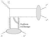
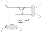
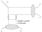
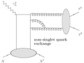
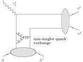
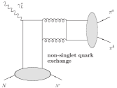
Figure 1: Typical NLO diagrams for di-pion production in the isovector (upper line) and isoscalar (lower line) state. The diagrams related to each other by crossing are displayed one upon another.

Due to charge conjugation invariance the production of an isovector pion pair, described by a $C$ odd quark DA, is mediated by gluon and $C$ even quark GPDs, $F^{g}$ and $F^{(+)}$. In contrast, the $C$ odd quark GPD $F^{(-)}$ contributes for the production of an isoscalar pion pair, which is produced by hadronization of a a gluon pair or a $C$ even quark pair.

The coefficient functions represent the amplitudes for the scattering of collinear partons. Typical NLO diagrams are shown in Fig. 1, where the graphs in the first, the second and the third columns contribute to $R^{(\pm)},G^{(\pm)}$ and $Q^{(\pm)}$ respectively. $R^{(+)},G^{(+)},Q^{(+)}$ were calculated in the $\overline{\textrm{MS}}$ scheme in [8], where electroproduction of light vector mesons was studied at NLO. For example

$$R^{(+)}(z,\tau)=\alpha_{s}^{2}(\mu_{R}^{2})C_{F}\frac{\displaystyle 1}{\displaystyle 8\pi z\bar{z}}{\cal R}\left(z,\frac{\tau-\xi}{2\xi}\right)\,,$$ (6)

$${\cal R}(z,y)=\Biggl{\{}\frac{2y+1}{y(y+1)}\left[\frac{y}{2}\ln^{2}(-y)-\frac{y+1}{2}\ln^{2}(y+1)+\left(\ln\left(\frac{Q^{2}z}{\mu_{F}^{2}}\right)-1\right)\left(y\ln(-y)-(y+1)\ln(y+1)\right)\right]$$

$$-\frac{V(z,y)}{y+z}+\frac{y\ln(-y)+(y+1)\ln(y+1)}{y(y+1)}+\frac{y(y+1)+(y+z)^{2}}{(y+z)^{2}}W(z,y)\Biggr{\}}+\Biggl{\{}z\rightarrow\bar{z}\Biggr{\}}\,,$$

where $\mu_{R}\,(\mu_{F})$ is the normalization (factorization) scale, $C_{F}=(N_{c}^{2}-1)/2N_{c}$, and

$$V(z,y)=z\ln(-y)+\bar{z}\ln(y+1)+z\ln(z)+\bar{z}\ln(\bar{z})$$

$$W(z,y)=\mathrm{Li}_{2}(y+1)-\mathrm{Li}_{2}(-y)+\mathrm{Li}_{2}(z)-\mathrm{Li}_{2}(\bar{z})+\ln(-y)\ln(\bar{z})-\ln(y+1)\ln(z)\,.$$

The hard amplitudes for pion production in the isoscalar state can be obtained by crossing from those for the isovector state. They correspond to each other after the interchange of the $t$-channel and the $s$-channel partonic pairs and the appropriate interchange of the relative partonic momentum fractions. One can convince oneself of this relationship easily by comparing the typical NLO diagrams on the upper and lower line in the Fig. 1. The prescription for the interchange of the momentum fractions reads

$$z\leftrightarrow\frac{\xi+\tau}{2\xi}\,,\quad\bar{z}\leftrightarrow\frac{\xi-\tau}{2\xi}\,,$$ (7)

then $Q^{(-)}\left(z,\tau\right)=Q^{(+)}\left(\frac{\xi+\tau}{2\xi},\xi(2z-1)\right)$, and similar relations hold for $R^{(-)},G^{(-)}$.

3 Numerical results

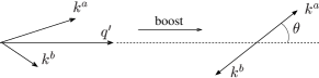
Figure 2: Definition of the polar angle $\theta$ in the c.m. of the pion pair.

We will present results for normalized Legendre moments (NLMs) defined as a convolution of differential cross section

$$\langle{P_{n}(\cos\theta)}\rangle^{\pi^{a}\pi^{b}}=\frac{\int\limits_{-1}^{1}\mathrm{d}\cos\theta\,\;{P_{n}(\cos\theta)}\,\frac{\mathrm{d}\sigma^{\pi^{a}\pi^{b}}}{\mathrm{d}\cos\theta}}{\int\limits_{-1}^{1}\mathrm{d}\cos\theta\,\;\frac{\mathrm{d}\sigma^{\pi^{a}\pi^{b}}}{\mathrm{d}\cos\theta}}$$ (8)

with a Legendre polynomial $P_{n}(\cos\theta)$, where the polar angle $\theta$ is defined in Fig. 2.

The GPDs in our calculation are modeled using the ansatz for double distributions suggested by Radyushkin [9]. Our models for 2$\pi$DAs reads

$$\Phi^{I=1}(z,\zeta,m_{\pi\pi})=6z(1-z)(2\zeta-1)F_{\pi}(m_{\pi\pi})\,,$$ (9)

$${\Phi^{I=0}(z,\zeta,m_{\pi\pi})=}-\frac{120M_{2}^{Q}}{n_{f}}z(1-z)(2z-1)\left[\frac{3-\beta^{2}}{12}f_{0}(m_{\pi\pi})P_{0}(\cos\theta)-\frac{\beta^{2}}{6}f_{2}(m_{\pi\pi})P_{2}(\cos\theta)\right]\,,$$

$${\Phi^{G}(z,\zeta,m_{\pi\pi})=}-60M_{2}^{G}z^{2}(1-z)^{2}\left[\frac{3-\beta^{2}}{12}f_{0}(m_{\pi\pi})P_{0}(\cos\theta)-\frac{\beta^{2}}{6}f_{2}(m_{\pi\pi})P_{2}(\cos\theta)\right]\,,$$

where $2\zeta-1=\beta\cos\theta$, the pion velocity in the di-pion c.m. is $\beta=\sqrt{1-4m^{2}_{\pi}/m^{2}_{\pi\pi}}$, and $n_{f}$ is the number of active flavors. $M_{2}^{Q}$ and $M_{2}^{G}$ represent the momentum fractions carried by quarks and gluons in the pion target. The isovector pair is produced in a $P$-wave, and $F_{\pi}(m_{\pi\pi})$ is the timelike electromagnetic pion form factor. The isoscalar pair may be in an $S$- or $D$-waves, and $f_{0}(m_{\pi\pi})$ and $f_{2}(m_{\pi\pi})$ are the corresponding Omnès functions for $S$- and $D$-waves. Omnès functions develop an imaginary part above two-pion threshold. In the region where pion-pion scattering is elastic, the phases of $f_{0}(m_{\pi\pi})$ and $f_{2}(m_{\pi\pi})$ coincide with the pion phase shifts $\delta_{0}^{I=0}$, $\delta_{2}^{I=0}$ (Watson theorem). For more details see [10, 5]. For higher di-pion masses the phases of Omnès functions do not coincide with the pion phase shifts. In the present analysis we neglect inelasticity and use the pion phase shifts as an input in dispersion relations to reconstruct the Omnès functions. We use two sets (S1 and S2) of parameterizations for the Omnès functions. In the set S1 we calculate Omnès functions using dispersion relations with two subtractions and the fits [11] for the pion phase shifts. For the subtraction constant we used the result of [10]. The set S2 is the same as that one used in [6].

Odd Legendre moments are proportional to the product of isoscalar and isovector amplitudes

$$\langle P_{1,3}\rangle\propto\int d\cos\theta\,\,P_{1,3}(\cos\theta)\,Re\left\{\left(T^{I=1}\right)^{*}T^{I=0}\right\}$$ (10)

and sensitive to the interference of $P$-wave with $S$- or $D$- wave,

$$\langle P_{1}\rangle\propto Re\left\{F^{*}_{\pi}(m_{\pi\pi})(c_{1}f_{0}(m_{\pi\pi})+c_{2}f_{2}(m_{\pi\pi}))\right\}\,,\quad\langle P_{3}\rangle\propto Re\left\{F^{*}_{\pi}(m_{\pi\pi})f_{2}(m_{\pi\pi})\right\}\,.$$ (11)

These observables provide access to a small isoscalar amplitude.

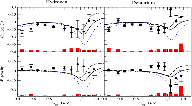
Figure 3: The $m_{\pi\pi}$ dependence of the normalized Legendre moments $\langle P_{1}\rangle$ (upper panels) and $\langle P_{3}\rangle$ (lower panels) for hydrogen (left panels) and deuterium (right panels). The curves show our results at LO (dashed black), NLO (solid black) and at NLO without two-gluon exchange in the $t$-channel (dotted). The average kinematics for the HERMES data [4] is $\langle x_{\mathrm{Bj}}\rangle=0.16$, $\langle Q^{2}\rangle=3.2\,(3.3)\,\textrm{GeV}^{2}$, and $\langle-t\rangle=0.43\,(0.29)\,\textrm{GeV}^{2}$ for hydrogen (deuterium). The histograms show the systematic uncertainty of the measurement.

In Fig. 3 we compare the results of our calculation (with set S1) with HERMES data for NLMs on hydrogen and deuterium targets [4]. Note that the difference between the LO and NLO results is not big, which may indicate a fast convergence of the perturbative series. Our leading twist predictions for $P_{1}$ are in reasonable agreement with the experimental data for the hydrogen and deuterium targets. Since such experiments in principle allow one to test the gluonic content of the nucleon, we plot in addition the corresponding results when we omit the two-gluon exchange in the $t$-channel. The effect of the gluon contribution is noticeable, hence improved data in the future may provide constraints on the gluonic content of the nucleon.

In Fig. 4 we present our results for kinematics typical of the COMPASS experiment, i.e. for larger $Q^{2}$ and smaller $x_{\rm{Bj}}$. We plot here the results obtained with different Omnès functions, with and without account of two-gluon exchange the $t$-channel. The predicted values of the NLMs are smaller for COMPASS kinematics than that ones for HERMES. Another observation is that the gluon GPD plays here even a more important role.

Figure 4: The normalized Legendre moments calculated for a deuterium target in the kinematic region relevant for COMPASS ( $x_{\mathrm{Bj}}=0.08$, $-t=0.27\,\textrm{GeV}^{2}$ and $Q^{2}=7\,\textrm{GeV}^{2}$) with sets S1 (solid) and S2 (dashed lines). The dotted and dashed-dotted lines represent the calculation without two-gluon exchange in the $t$-channel, for sets S1 and S2 respectively.

To estimate the scale uncertainties of our NLO calculation we plot in Fig. 5 for HERMES kinematics the ”longitudinal” combination of the moments, which projects out the state with vanishing total helicity of the pion pair, calculated with set S1 and different settings in the hard part for the factorization and the renormalization scales. We see that this scale uncertainty is not large.

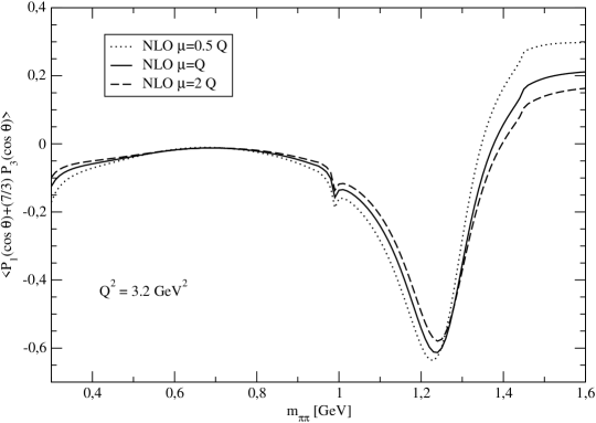
Figure 5: The ”longitudinal” NLM combination calculated for different renormalization and factorization scales, $\mu_{R}=\mu_{F}=\mu$.

4 Summary

We studied di-pion electroproduction in the QCD factorization approach at NLO. Numerical results obtained for HERMES and COMPASS kinematics show that NLO corrections (at least for normalized Legendre moments) are small. Hence with improved experimental data from such experiments it will be possible to put the constrains on both GPDs and 2$\pi$DAs. One can also get additional insight into the gluonic content of the nucleon. To be on the safe side with the leading twist approach it is, however, important to go to larger $Q^{2}$.

In the future we want to improve our approach to Omnès functions by taking into account inelasticity effects.

References

- [1] K. Goeke, M.V. Polyakov and M. Vanderhaeghen, Prog. Part. Nucl. Phys. 47 (2001) 401.
- [2] M. Diehl, Phys. Rept. 388 (2003) 41.
- [3] A.V. Belitsky and A.V. Radyushkin, Phys. Rept. 418 (2005) 1.
- [4] A. Airapetian et al. [HERMES Collaboration], Phys. Lett. B 599 (2004) 212.
- [5] B. Lehmann-Dronke, P.V. Pobylitsa, M.V. Polyakov, A. Schafer and K. Goeke, Phys. Lett. B 475 (2000) 147.
- [6] B. Lehmann-Dronke, A. Schaefer, M.V. Polyakov and K. Goeke, Phys. Rev. D 63 (2001) 114001.
- [7] J.C. Collins, L. Frankfurt and M. Strikman, Phys. Rev. D 56 (1997) 2982.
- [8] D.Yu. Ivanov, L. Szymanowski and G. Krasnikov, JETP Lett. 80 (2004) 226 [Pisma Zh. Eksp. Teor. Fiz. 80 (2004) 255].
- [9] A.V. Radyushkin, Phys. Rev. D 59 (1999) 014030.
- [10] M.V. Polyakov, Nucl. Phys. B 555 (1999) 231.
- [11] J.R. Pelaez and F.J. Yndurain, Phys. Rev. D 71 (2005) 074016.