Clues for the existence of two $K_{1}(1270)$ resonances

Abstract

The axial vector meson $K_{1}(1270)$ was studied within the chiral unitary approach, where it was shown that it has a two-pole structure. We reanalyze the high-statistics WA3 experiment $K^{-}p\rightarrow K^{-}\pi^{+}\pi^{-}p$ at 63 GeV, which established the existence of both $K_{1}(1270)$ and $K_{1}(1400)$, and we show that it clearly favors our two-pole interpretation. We also reanalyze the traditional K-matrix interpretation of the WA3 data and find that the good fit of the data obtained there comes from large cancellations of terms of unclear physical interpretation.

I Introduction

Two nonets of spin-parity $1^{+}$ mesons are expected on the basis of $L=1$ excitation of $q\bar{q}$ system. According to the particle data group (PDG) Yao:2006px , they are $b_{1}(1235)$, $h_{1}(1170)$, $h_{1}(1380)$, $a_{1}(1260)$, $f_{1}(1285)$, $f_{1}(1420)$, $K_{1}(1270)$ and $K_{1}(1400)$. Due to SU(3) breaking, as the mass of the $s$ quark is larger than those of the $u$ and $d$ quarks, the $K_{1}(1270)$ and $K_{1}(1400)$ are assumed to be a mixture of the SU(3) eigenstates $K_{1B}$ with $C=-1$ and $K_{1A}$ with $C=+1$. Thus, they provide a possibility to understand the SU(3) symmetry breaking in the non-perturbative regime. Particularly important in this respect is the mixing angle $\theta_{K}$ between the two SU(3) eigenstates. In the literature, different approaches have been adopted to determine its value using various experimental inputs, but a consensus is not yet reached. Recent BES data even call for two different values to explain the data, $\theta_{K}<29\hbox{${}^{\circ}$}$ for $\psi(2S)$ decay and $\theta_{K}>48\hbox{${}^{\circ}$}$ for $J/\psi$ decay Bai:1999mq . This issue might become even more complicated as shown in a recent theoretical study that there might be two poles for $K_{1}(1270)$ Roca:2005nm –a scenario similar to that of $\Lambda(1405)$ Magas:2005vu . In the present work, we aim to explore the possible experimental consequence of such a two-pole structure.

The $Q$ mesons, i.e. $K_{1}(1270)$ and $K_{1}(1400)$ as known today, have been observed in $\bar{p}p$ annihilation at rest Armenteros64 ; Astier:1969dt , the coherent reaction $K^{+}d\rightarrow K^{+}\pi^{+}\pi^{-}d$ Firestone:1972st , the baryon exchange reaction $K^{-}p\rightarrow\Xi^{-}(K\pi\pi)^{+}$ Gavillet:1978rj , the hypercharge exchange reaction $\pi^{-}p\rightarrow(K\pi\pi)\Lambda$ Rodeback:1980zt , the diffractive productions $K^{\pm}p\rightarrow K^{\pm}\pi^{+}\pi^{-}p$ Brandenburg:1975gv ; Daum:1981hb , and more lately, in the decay of $\psi(2S)$ into $K_{1}(1270)$ and $K_{1}(1400)$ by BES collaboration Bai:1999mq , the exclusive decay process $B\rightarrow J/\psi K_{1}(1270)$ by Belle collaboration Abe:2001wa , the mass spectrum and resonant structure in $\tau^{-}\rightarrow K^{-}\pi^{+}\pi^{-}\nu_{\tau}$ decays by CLEO collaboration Asner:2000nx , and in the decay of $J/\psi\rightarrow K^{*}(890)K\pi$ Bugg:2005ni ; Ablikim:2005ni . The experimental evidence can be summarized as follows: in diffractive processes one often observes both $K_{1}(1270)$ and $K_{1}(1400)$ Otter:1976kk ; Daum:1981hb ; Brandenburg:1975gv . However, in non-diffractive processes (such as hypercharge exchange process Rodeback:1980zt and baryon exchange process Gavillet:1978rj ) one often observes only one resonance mostly in the $\rho K$ channel Rodeback:1980zt ; Gavillet:1978rj . It is interesting to stress that a two-peak structure has been observed in the $K^{*}\pi$ invariant mass spectrum Otter:1976kk ; Daum:1981hb ; Brandenburg:1975gv . In Ref. Daum:1981hb , the two peaks appear at $\sim 1240$ MeV and $\sim 1400$ MeV. While in Ref. Brandenburg:1975gv , the two peaks appear at $\sim 1200$ MeV and $\sim 1400$ MeV. The two peaks of G. Otter et al. Otter:1976kk , on the other hand, appear at $\sim 1.27$ GeV and $\sim 1.37$ GeV. While such a structure is hardly seen in the $K^{-}p$ reaction at 4.2 GeV$/c$ Vergeest:1979jd . Thus, the two-peak structure is clearly related to the reaction energy. It seems to be more prominent in high energy $K^{\pm}p$ reactions than in low energy reactions.

It should be stressed that the most conclusive and high-statistics data of $K_{1}(1270)$ come from the WA3 experiment at CERN that accumulated data on the reaction $K^{-}p\to K^{-}\pi^{+}\pi^{-}p$ at 63 GeV. These data were analyzed by the ACCMOR Collaboration Daum:1981hb . As will be shown in this paper, the two-peak structure, with a peak at lower energy depending drastically on the reaction channel investigated, can be easily explained in our model with two poles for $K_{1}(1270)$ plus the $K_{1}(1400)$. With only one pole, as has been noted long time ago Bowler:1976qe ; Daum:1981hb , there is always a discrepancy for the peak positions observed in the $K^{*}\pi$ and $\rho K$ invariant mass distributions. In the present work, we mainly concentrate our study on the WA3 data Daum:1981hb . Other data have been carefully studied, but since they either have too few events or too much background, no direct contrast of our analysis with these data will be presented.

Nowadays, it is generally accepted that QCD is the underlying theory of strong interactions. Due to the asymptotic freedom, however, its application at low energies around 1 GeV is highly problematic. Therefore, various effective theories have been employed. Chiral symmetry, related with small $u$, $d$, $s$ masses, provides a general principle for constructing effective field theory to study low-energy phenomena. In this respect, Chiral perturbation theory has been rather successful in studies of low-energy hadron phenomena Weinberg:1978kz ; Gasser:1984gg ; Meissner:1993ah ; Bernard:1995dp ; Pich:1995bw ; Ecker:1994gg . However, pure perturbation theory cannot describe the low-lying resonances. The breakthrough came with the application of unitary techniques in the conventional chiral perturbation theory, enabling one to study higher energy regions hitherto unaccessible, while employing chiral Lagrangians. The unitary extension of chiral perturbation theory, U$\chi$PT, has been successfully applied to study meson-baryon and meson-meson interactions. More recently, it has been used to study the lowest axial vector mesons $b_{1}(1235)$, $h_{1}(1170)$, $h_{1}(1380)$, $a_{1}(1260)$, $f_{1}(1285)$, $K_{1}(1270)$ and $K_{1}(1400)$ Lutz:2003fm ; Roca:2005nm . Both works generate most of the low-lying axial vector mesons dynamically but differ in one thing: In Ref. Lutz:2003fm , the authors claimed to have found both $K_{1}(1270)$ and $K_{1}(1400)$, while in Ref. Roca:2005nm , no signal was found for $K_{1}(1400)$. In addition, in Ref. Roca:2005nm the two poles appearing on the second Riemann sheet were both attributed to $K_{1}(1270)$ due to the considerations of pole positions and main decay channels. One should be aware that only for low energies U$\chi$PT can be considered model independent (either for meson-meson, meson-baryon or baryon-baryon scattering), and it incorporates the basic symmetries and dynamical features of QCD, among them chiral symmetry with its symmetry breaking patterns. At higher energies, the perturbative method of $\chi$PT is no longer applicable and what U$\chi$PT does is to provide an extrapolation of $\chi$PT at higher energies by imposing two restrictions: matching $\chi$PT at low energies and implementing unitarity in coupled channels in an exact way. These two restrictions give little freedom to the amplitudes, basically a few subtraction constants in the dispersion relations which are fitted to experiment.

This paper is organized as follows. In Section II, we briefly describe the unitary chiral approach. We also explain how we treat the finite widths of vector mesons. An empirical study is performed in Section III on the WA3 data. It is demonstrated that the WA3 data can be well explained by our two-pole structure for $K_{1}(1270)$. In Section IV, we analyze the K-matrix approach which has long been used to study the diffractive production of $Q$ mesons. We point out that although this approach can reproduce the data very well, the results seem to be unstable and not very meaningful physically. In Section V, we demonstrate that the most important channels to describe the WA3 data are the $K^{*}\pi$ and $\rho K$ channels. A brief summary is given in Section VI.

II Chiral unitary approach

The detailed formalism has been given in Ref. Roca:2005nm . In the following, we only provide a brief introduction for the sake of completeness. In the literature, several unitarization procedures have been used to obtain a scattering matrix fulfilling exact unitarity in coupled channels, such as the Inverse Amplitude Method Dobado:1996ps ; Oller:1997ng ; Oller:1998hw or the $N/D$ method Oller:1998zr . In this latter work the equivalence with the Bethe-Salpeter equation used in Oller:1997ti was established.

In the present work we make use of the Bethe-Salpeter approach, which leads to the following unitarized amplitude:

$$T=[1+V\hat{G}]^{-1}(-V)\,\vec{\epsilon}\cdot\vec{\epsilon}\,^{\prime},$$ (1)

where $\hat{G}=(1+\frac{1}{3}\frac{q^{2}_{l}}{M_{l}^{2}})G$ is a diagonal matrix with the $l-$th element, $G_{l}$, being the two meson loop function containing a vector and a pseudoscalar meson:

$$G_{l}(\sqrt{s})=i\,\int\frac{d^{4}q}{(2\pi)^{4}}\,\frac{1}{(P-q)^{2}-M_{l}^{2}+i\epsilon}\,\frac{1}{q^{2}-m^{2}_{l}+i\epsilon},$$ (2)

with $P$ the total incident momentum, which in the center of mass frame is $(\sqrt{s},0,0,0)$. In the dimensional regularization scheme the loop function of Eq. (2) gives

$$G_{l}(\sqrt{s}) = \frac{1}{16\pi^{2}}\left\{a(\mu)+\ln\frac{M_{l}^{2}}{\mu^{2}}+\frac{m_{l}^{2}-M_{l}^{2}+s}{2s}\ln\frac{m_{l}^{2}}{M_{l}^{2}}\right.$$ (3)

$$\phantom{\frac{1}{16\pi^{2}}}+\frac{q_{l}}{\sqrt{s}}\left[\ln(s-(M_{l}^{2}-m_{l}^{2})+2q_{l}\sqrt{s})+\ln(s+(M_{l}^{2}-m_{l}^{2})+2q_{l}\sqrt{s})\right.$$

$$\left.\phantom{\frac{1}{16\pi^{2}}+\frac{q_{l}}{\sqrt{s}}}\left.-\ln(-s+(M_{l}^{2}-m_{l}^{2})+2q_{l}\sqrt{s})-\ln(-s-(M_{l}^{2}-m_{l}^{2})+2q_{l}\sqrt{s})\right]\right\},$$

where $\mu$ is the scale of dimensional regularization. Changes in the scale are reabsorbed in the subtraction constant $a(\mu)$, so that the results remain scale independent. In Eq. (3), $q_{l}$ denotes the three-momentum of the vector or pseudoscalar meson in the center of mass frame.

The tree level amplitudes are calculated using the following interaction Lagrangian Birse:1996hd :

$${\cal L}_{I}=-\frac{1}{4}\mathrm{Tr}\left\{\left(\nabla_{\mu}V_{\nu}-\nabla_{\nu}V_{\mu}\right)\left(\nabla^{\mu}V^{\nu}-\nabla^{\nu}V^{\mu}\right)\right\},$$ (4)

where $\mathrm{Tr}$ means SU(3) trace and $\nabla_{\mu}$ is the covariant derivative defined as

$$\nabla_{\mu}V_{\nu}=\partial_{\mu}V_{\nu}+[\Gamma_{\mu},V_{\nu}],$$ (5)

where $[,]$ stands for commutator and $\Gamma_{\mu}$ is the vector current

$$\Gamma_{\mu}=\frac{1}{2}(u^{\dagger}\partial_{\mu}u+u\partial_{\mu}u^{\dagger})$$ (6)

with

$$u^{2}=U=e^{i\frac{\sqrt{2}}{f}P}.$$ (7)

In the above equations $f$ is the pion decay constant in the chiral limit and $P$ and $V$ are the SU(3) matrices containing the octet of pseudoscalar and the nonet of vector mesons respectively:

$$P\equiv\left(\begin{array}[]{ccc}\frac{1}{\sqrt{2}}\pi^{0}+\frac{1}{\sqrt{6}}\eta_{8}&\pi^{+}&K^{+}\\ \pi^{-}&-\frac{1}{\sqrt{2}}\pi^{0}+\frac{1}{\sqrt{6}}\eta_{8}&K^{0}\\ K^{-}&\bar{K}^{0}&-\frac{2}{\sqrt{6}}\eta_{8}\end{array}\right),$$ (8)

$$V_{\mu}\equiv\left(\begin{array}[]{ccc}\frac{1}{\sqrt{2}}\rho^{0}+\frac{1}{\sqrt{2}}\omega&\rho^{+}&K^{*+}\\ \rho^{-}&-\frac{1}{\sqrt{2}}\rho^{0}+\frac{1}{\sqrt{2}}\omega&K^{*0}\\ K^{*-}&\bar{K}^{*0}&\phi\end{array}\right)_{\mu}.$$ (9)

Table 1: $C_{ij}$ coefficients in isospin basis for the $S=1$, $I=\frac{1}{2}$ channel.

	$\phi K$	$\omega K$	$\rho K$	$K^{*}\eta$	$K^{*}\pi$
$\phi K$	$0$	$0$	$0$	$-\sqrt{\frac{3}{2}}$	$-\sqrt{\frac{3}{2}}$
$\omega K$	$0$	$0$	$0$	$\frac{\sqrt{3}}{2}$	$\frac{\sqrt{3}}{2}$
$\rho K$	$0$	$0$	$-2$	$-\frac{3}{2}$	$\frac{1}{2}$
$K^{*}\eta$	$-\sqrt{\frac{3}{2}}$	$\frac{\sqrt{3}}{2}$	$-\frac{3}{2}$	$0$	$0$
$K^{*}\pi$	$-\sqrt{\frac{3}{2}}$	$\frac{\sqrt{3}}{2}$	$\frac{1}{2}$	$0$	$-2$

The two-vector–two-pseudoscalar amplitudes can be obtained by expanding the Lagrangian of Eq. (4) up to two pseudoscalar meson fields:

$${\cal L}_{VVPP}=-\frac{1}{4f^{2}}\mathrm{Tr}\left([V^{\mu},\partial^{\nu}V_{\mu}][P,\partial_{\nu}P]\right),$$ (10)

which would account for the Weinberg-Tomozawa interaction for the $VP\to VP$ process Birse:1996hd ; Lutz:2003fm . As in Ref. Roca:2005nm in the pseudoscalar octet we assume $\eta_{8}\equiv\eta$. In the vector meson multiplet, ideal $\omega_{1}-\omega_{8}$ mixing is assumed:

$$\phi=\omega_{1}/\sqrt{3}-\omega_{8}\sqrt{2/3},\quad\omega=\omega_{1}\sqrt{2/3}+\omega_{8}/\sqrt{3}.$$ (11)

Throughout the work, the following phase convention is used: $|\pi^{+}\rangle=-|1+1\rangle$, $|\rho^{+}\rangle=-|1+1\rangle$, $|K^{-}\rangle=-|1/2-1/2\rangle$ and $|K^{*-}\rangle=-|1/2-1/2\rangle$ with the notation $|II_{3}\rangle$ to denote isospin states.

From the Lagrangian of Eq. (10) one obtains the $s$-wave amplitude:

$$V_{ij}(s) = -\frac{\epsilon\cdot\epsilon^{\prime}}{8f^{2}}C_{ij}\left[3s-(M^{2}+m^{2}+M^{\prime 2}+m^{\prime 2})\right.$$ (12)

$$\left.\hskip 42.67912pt-\frac{1}{s}(M^{2}-m^{2})(M^{\prime 2}-m^{\prime 2})\right],$$

where $\epsilon$($\epsilon^{\prime}$) stands for the polarization four-vector of the incoming(outgoing) vector meson. The masses $M(M^{\prime})$, $m(m^{\prime})$ correspond to the initial(final) vector mesons and initial(final) pseudoscalar mesons respectively, and we use an averaged value for each isospin multiplet. The indices $i$ and $j$ represent the initial and final $VP$ states respectively. The $C_{ij}$ coefficients for the $(S,I)=(1,1/2)$ $VP$ channel are tabulated in Table 1.

In Ref. Roca:2005nm , the finite widths of vector mesons are not taken into account in the dimensional regularization scheme. They are only considered in the cut-off scheme. In the present work, we take into account the finite widths of vector mesons in the dimensional regularization scheme. The precise analytical structure of the scheme allows us to calculate the pole positions on the second Riemann sheet. As we will show below, the main effect of the widths of vector mesons is to modify the widths of the two poles of $K_{1}(1270)$. Since the tree level amplitudes $V$ do not contribute to the resonances, the widths of the vector mesons contribute through the momentum $q$ and loop function $G$. The appropriate way to implement this, respecting the unitarity implicit in the Bethe-Salpeter equation, is to substitute in Eq. (2) the propagator of the unstable particle by its exact propagator, incorporating a self-energy that accounts for all the decay channels through its imaginary part. This is most efficiently done by means of the Lehmann representation which writes the propagator in terms of its imaginary part

$$D(s)=\int^{\infty}_{s_{\mathrm{th}}}ds_{V}(-\frac{1}{\pi})\frac{\mathrm{Im}\,D(s_{V})}{s-s_{V}+i\epsilon}$$ (13)

with $s={q^{0}}^{2}-\vec{q}\,^{2}$ and $s_{\mathrm{th}}$ the threshold for decay channels, and then we take the spectral function for the propagator $\mathrm{Im}\,D(s_{V})$ as

$$\mathrm{Im}\,D(s_{V})=\mathrm{Im}\left\{\frac{1}{s_{V}-M^{2}_{V}+iM_{V}\Gamma_{V}}\right\}$$ (14)

where we indulge in the approximation of taking $\Gamma_{V}$ as constant instead of the explicit function of $s_{V}$, which would require detailed study of all the decay channels. This further sophisticated step is unnecessary here, inducing changes far smaller than the uncertainties of the approach from other sources discussed in Ref. Roca:2005nm . By using Eq. (13) the loop function of Eq. (2) now reads

$$G_{l}(\sqrt{s},M_{l},m_{l})=\frac{1}{C}\int\limits^{(M_{V}+2\Gamma_{V})^{2}}_{(M_{V}-2\Gamma_{V})^{2}}ds_{V}\times G(\sqrt{s},\sqrt{s_{V}},m_{l})\times\left(-\frac{1}{\pi}\right)\mathrm{Im}\left\{\frac{1}{s_{V}-M^{2}_{V}+iM_{V}\Gamma_{V}}\right\}$$ (15)

with

$$C=\int\limits^{(M_{V}+2\Gamma_{V})^{2}}_{(M_{V}-2\Gamma_{V})^{2}}ds_{V}\times\left(-\frac{1}{\pi}\right)\mathrm{Im}\left\{\frac{1}{s_{V}-M^{2}_{V}+iM_{V}\Gamma_{V}}\right\}$$ (16)

where a reasonable cut, $M_{V}\pm 2\Gamma_{V}$, is done in the $s_{V}$ integration and the constant $C$ is introduced to restore the small loss of renormalization of the Breit-Wigner distribution with this cut. A similar prescription has been applied to account for the dispersion of the momentum $q$ in some coming formulas.

In the chiral unitary model that we employed, the free parameters are the decay constant $f$ and the subtraction constant $a(\mu)$, which are highly correlated. We have checked that the two-pole structure remains very robust with respect to a reasonable readjustment of these parameters. On the other hand, the parameter values used in Ref. Roca:2005nm produce too low pole positions for $K_{1}(1270)$ (see Table 2).

Table 2: The pole positions and widths of $K_{1}(1270)$ obtained with the original parameters of Ref. Roca:2005nm . The constant $f$ is the pion decay constant in the chiral limit, $a(\mu)$ is the subtraction constant and $\mu$ is the renormalization scale. “Zero width” denotes the results obtained with sharp vector meson masses while “Finite width” denotes the results obtained by taking into account the finite widths of vector mesons. All energy units are in MeV.

			Zero width		Finite width
$f$	$a(\mu)$	$\mu$	1st pole position	2nd pole position	1st pole position	2nd pole position
92	$-1.85$	900	$(1111-i65)$	$(1216-i4)$	$(1111-i64)$	$(1210-i26)$

Therefore, we have readjusted these parameters to move the higher pole position closer to the nominal position of $K_{1}(1270)$. This can be most conveniently achieved by increasing $f$.

Figure 1: The modulus square of the coupled channel amplitudes in the $S=1$ and $I=\frac{1}{2}$ channel.

Figure 2: The modulus square of the coupled channel amplitudes multiplied by the corresponding loop functions in the $S=1$ and $I=\frac{1}{2}$ channel.

Figs. 1 and 2 show the modulus square of the $S=1$, $I=\frac{1}{2}$ amplitudes and those multiplied by the corresponding loop functions obtained with $f=115$ MeV, $a(\mu)=-1.85$ and $\mu=900$ MeV. The pole positions and corresponding widths obtained with this set of parameters are tabulated in Table 3.

Table 3: The same as Table 2, but with readjusted parameters.

			Zero width		Finite width
$f$	$a(\mu)$	$\mu$	1st pole position	2nd pole position	1st pole position	2nd pole position
115	$-1.85$	900	$(1199-i126)$	$(1271-i1)$	$(1195-i123)$	$(1284-i73)$

From Figs. 1 and 2, the two poles are clearly seen: the higher pole manifests itself as one relatively narrower resonance around 1.28 GeV and the lower pole as a broader resonance at $\sim 1.20$ GeV. Furthermore, these two poles couple to different channels quite differently. The higher pole is seen mostly in the $\rho K\rightarrow\rho K$ channel while the lower pole is mostly seen in the $K^{*}\pi\rightarrow K^{*}\pi$ channel. If different reaction mechanisms favor one or the other channel, they will see different shapes for the resonance. More importantly, it is to be noted that not only the two poles couple to different channels with different strengths, but also they manifest themselves in different final states. In other words, in the $\rho K$ final states, one favors a narrower resonance around 1.28 GeV, while in the $K^{*}\pi$ final states, one would favor a broader resonance at a smaller invariant mass.

As pointed out in Ref. Roca:2005nm , close to a pole, the $T$ matrix amplitude on the second Riemann sheet can be expressed, removing the trivial $\epsilon\cdot\epsilon^{\prime}$ which is also absent in the other amplitudes, as

$$T_{ij}=\frac{g_{i}g_{j}}{s-s_{p}}$$ (17)

where $s$ is the energy squared in the center of mass frame and $\sqrt{s_{p}}$ the pole position. The numbers $g_{i}$($g_{j}$) can be understood as the effective couplings of the dynamically generated resonance to channel $i$($j$). They can be calculated from the residues of the amplitudes at the complex pole positions. The effective couplings for $\phi K$, $\omega K$, $\rho K$, $K^{*}\eta$ and $K^{*}\pi$ are tabulated in Table 4 for both the lower pole and the higher pole, respectively.

Table 4: Effective couplings of the two poles of $K_{1}(1270)$ to the five channels: $\phi K$, $\omega K$, $\rho K$, $K^{*}\eta$ and $K^{*}\pi$. All the units are in MeV.

$\sqrt{s_{p}}$	$1195-i123$		$1284-i73$
	$g_{i}$	$|g_{i}|$	$g_{i}$	$|g_{i}|$
$\phi K$	$2096-i1208$	$2420$	$1166-i774$	$1399$
$\omega K$	$-2046+i821$	$2205$	$-1051+i620$	$1220$
$\rho K$	$-1671+i1599$	$2313$	$4804+i395$	$4821$
$K^{*}\eta$	$72+i197$	$210$	$3486-i536$	$3526$
$K^{*}\pi$	$4747-i2874$	$5550$	$769-i1171$	$1401$

It is easily seen that the lower pole couples more dominantly to the $K^{*}\pi$ channel while the higher pole couples more strongly to the $\rho K$ channel. We note that these couplings do not differ qualitatively from those listed in Table IX of Ref. Roca:2005nm , although here we have readjusted $f$ from 92 MeV to 115 MeV and have taken into account the finite widths of vector mesons in the dimensional regularization scheme while they were accounted for in the cutoff method in Ref. Roca:2005nm .

III An empirical study of the WA3 data

As we mentioned in the introduction, the WA3 experiment $K^{-}p\rightarrow K^{-}\pi^{+}\pi^{-}p$ at 63 GeV is one of the most conclusive and high-statistics experiment on $K_{1}(1270)$. In this section, we analyze the WA3 data by constructing production amplitudes from the $t$ matrix amplitudes obtained in the above section. The reaction $K^{-}p\rightarrow K^{-}\pi^{+}\pi^{-}p$ can be analyzed by the isobar model as $K^{-}p\rightarrow(\bar{K}^{*0}\pi^{-}\,\mbox{or}\,\rho^{0}K^{-})p\rightarrow K^{-}\pi^{+}\pi^{-}p$. Therefore, we can construct the following amplitudes to simulate this process. Assuming $I=\frac{1}{2}$ dominance for $\bar{K}^{*0}\pi^{-}$ and $\rho^{0}K^{-}$ as suggested by the experiment we have

$$T_{K^{*}\pi}\equiv T_{\bar{K}^{*0}\pi^{-}} = \sqrt{\frac{2}{3}}a+\sqrt{\frac{2}{3}}aG_{K^{*}\pi}t_{K^{*}\pi\rightarrow K^{*}\pi}+\sqrt{\frac{2}{3}}bG_{\rho K}t_{\rho K\rightarrow K^{*}\pi},$$

$$T_{\rho K}\equiv T_{\rho^{0}K^{-}} = -\sqrt{\frac{1}{3}}b-\sqrt{\frac{1}{3}}aG_{K^{*}\pi}t_{K^{*}\pi\rightarrow\rho K}-\sqrt{\frac{1}{3}}bG_{\rho K}t_{\rho K\rightarrow\rho K},$$ (18)

where $t_{ij}$ are the coupled channel amplitudes obtained in Section II and the Clebsch-Gordan coefficient $\sqrt{\frac{2}{3}}$($-\sqrt{\frac{1}{3}}$) accounts for projecting the $I=\frac{1}{2}$ $K^{*}\pi$ ($\rho K$) state into $\bar{K}^{*0}\pi^{-}$($\rho^{0}K^{-}$). The coefficients $a$ and $b$ are complex couplings. In the most general case, $a$ and $b$ might also depend on energy. It should be noted that in our chiral unitary model there are five channels, while in constructing the above amplitudes, we have only considered two channels $K^{*}\pi$ and $\rho K$ due to the following consideration. These two channels are relatively more important than the other three as can be clearly seen from Fig. 2. In the $\rho K$ channel, $|G_{K^{*}\eta}t_{K^{*}\eta\rightarrow\rho K}|^{2}$ is of similar magnitude as that of $|G_{K^{*}\pi}t_{K^{*}\pi\rightarrow\rho K}|^{2}$, but both are much smaller than $|G_{\rho K}t_{\rho K\rightarrow\rho K}|^{2}$. Therefore, we expect in the $\rho K$ channel, one will almost always observe a narrow resonance at $\sim 1280$ MeV. Similar argument can be made about the $K^{*}\pi$ channel. This consideration allows us to reduce the number of free parameters, which would otherwise increase linearly with the number of channels included.

To contrast our model with data, it is necessary for us to take into account the existence of $K_{1}(1400)$, which is not dynamically generated in our approach. Therefore, we add to the amplitudes in Eq. (18) an explicit contribution of $K_{1}(1400)$

$$T_{K^{*}\pi} \rightarrow T_{K^{*}\pi}+\frac{g_{K^{*}\pi}}{s-M^{2}+iM\Gamma(s)},$$

$$T_{\rho K} \rightarrow T_{\rho K}+\frac{g_{\rho K}}{s-M^{2}+iM\Gamma(s)},$$ (19)

where $g_{K*\pi}$ and $g_{\rho K}$ are complex couplings, and $M$ and $\Gamma(s)$ are the mass and width of $K_{1}(1400)$ with the $s$-wave width given by

$$\Gamma(s)=\Gamma_{0}\frac{q(s)}{q_{\mathrm{on}}}\Theta(\sqrt{s}-M_{K^{*}}-M_{\pi}).$$ (20)

$q(s)$ and $q_{\mathrm{on}}$ are calculated by

$$q(s)=\frac{\lambda^{1/2}(s,M^{2}_{\pi},M^{2}_{K^{*}})}{2\sqrt{s}}\quad\mbox{and}\quad q_{\mathrm{on}}=\frac{\lambda^{1/2}(M^{2},M^{2}_{\pi},M^{2}_{K^{*}})}{2M}.$$ (21)

In our model, Eq. (19), we have the following adjustable parameters: $a$, $b$, $g_{K^{*}\pi}$, $g_{\rho K}$, $M$ and $\Gamma_{0}$. In principle, $f$ and $a(\mu)$ can also be taken as free parameters. In order to limit the number of free parameters, we have adopted the following procedure:

1. Starting from the values used in Ref. Roca:2005nm , we readjust $f$ slightly so that the higher pole position is close to the experimental $K_{1}(1270)$. This gives $f$ a value of $\sim 115$ MeV.

2. Since we have a global arbitrary phase, we take $a$ real while $b$ is kept complex.

3. $M$ and $\Gamma_{0}$ are fixed at their experimental values, i.e. $M=1402$ MeV and $\Gamma=174$ MeV. We note that a reasonable readjustment of these two values only gives a slightly better fit. Since this does not qualitatively improve our interpretation of the data, we are satisfied with fixed $M$ and $\Gamma$ (at the PDG values).

4. We minimize the difference between the WA3 data and our calculated amplitudes to fix the other seven parameters.

Figure 3: $K^{*}\pi$ and $\rho K$ invariant mass distributions. The data are from the WA3 reaction $K^{-}p\rightarrow K^{-}\pi^{+}\pi^{-}p$ at 63 GeV Daum:1981hb . Data in the upper panels are for $0\leq|t^{\prime}|\leq 0.05$ GeV² and those in the middle and bottom panels for $0.05\leq|t^{\prime}|\leq 0.7$ GeV², where $t^{\prime}$ is the four momentum transfer squared to the recoiling proton. The data are further grouped by $J^{P}LM^{\eta}$ followed by the isobar and odd particle. $J$ is the total angular momentum, $P$ the parity, $L$ the orbital angular momentum of the odd particle. $M^{\eta}$ denotes the magnetic substate of the $K\pi\pi$ system and the naturality of the exchange.

The results are shown in Fig. 3 in comparison with the WA3 data Daum:1981hb . According to Ref. Flatte:1976xu , for a $s$-wave resonance, the theoretical differential cross section can be calculated by

$$\frac{d\sigma}{dM}=c|T|^{2}q$$ (22)

where $M$ is the invariant mass of the $K^{*}\pi$ or $\rho K$ systems, $c$ is a normalization constant, $T$ is the amplitude specified above for the $K^{*}\pi$ or $\rho K$ channels and $q$ is the center of mass three-momentum of $K^{*}\pi$ or $\rho K$. We have taken $c$ to be 1, or in other words, it has been absorbed into the coupling constants $a$, $b$, $g_{K^{*}\pi}$ and $g_{\rho K}$, which are tabulated in Table 5.

Table 5: Parameter values obtained from fitting the WA3 data Daum:1981hb . Data set 1, 2, 3 correspond to the low $|t^{\prime}|$ $1^{+}S0^{+}$ data, the high $|t^{\prime}|$ $1^{+}S0^{+}$ data and the high $|t^{\prime}|$ $1^{+}S1^{+}$ data. The fits are performed by assigning an equal error of 100 (events) to each data point.

Data set	$a$	$b$	$g_{K*\pi}$ (MeV2)	$g_{\rho K}$ (MeV2)
1	1.65	($-1.60,0.27$)	($-221029,-341404)$	($-82631,-76119)$
2	$-1.41$	($0.31,-2.06)$	($536803,64738)$	($-13388,-219728)$
3	0.45	($-1.32,-0.24)$	($109352,-114341)$	($-179938,-46491)$

From Fig. 3, it is clearly seen that our model can fit the data around the peaks very well. In Fig. 3, the dashed and dotted lines are the separate contributions of $K_{1}(1270)$ and $K_{1}(1400)$. One can easily see that $K_{1}(1400)$ decays dominantly to $K^{*}\pi$, which is consistent with our present understanding of this resonance Yao:2006px .

It should be mentioned that in our model the lower peak observed in the invariant mass distribution of the $K^{*}\pi$ channel is due to the contribution of the two poles of $K_{1}(1270)$. This is very different from the traditional interpretation. For example, the lower peak observed in the $K^{*}\pi$ invariant mass distributions of $K^{\pm}p\rightarrow K^{\pm}\pi^{+}\pi^{-}p$ at 13 GeV was interpreted as a pure Gaussian background by Carnegie et al. Carnegie:1976cs , which has a shape similar to the contribution of the $K_{1}(1270)$ as shown in Fig. 3. On the other hand, the K-matrix approach was adopted to analyze the SLAC Brandenburg:1975gv and the WA3 data Daum:1981hb . In this latter approach, the lower peak mostly comes from the so-called Deck background, which after unitarization, also has a shape of resonance. As we mentioned in the introduction, even in the original WA3 paper Daum:1981hb , it was noted that their model failed to describe the $1^{+}S1^{+}$($K^{*}\pi$) data, in the notation $J^{P}LM^{\eta}$ with $\eta$ the naturality of the exchange Daum:1981hb . The predicted peak is 20 MeV higher than the data. If the fit were done only to the $K^{*}\pi$ data, the agreement was much better but then the predicted $K_{1}(1270)$ would be lower by 35 MeV than that obtained when other channels were also considered in the fit. We will discuss more about the K-matrix approach in the following section.

It is worth stressing that the $K_{1}(1270)$ peak seen in the upper-left panel of Fig. 3 is significantly broader than that in the upper-right panel. Furthermore the peak positions are also different in the two cases (1240 MeV and 1280 MeV respectively). Both features have a straightforward interpretation in our theoretical description since the first one is dominated by the low-energy (broader) $K_{1}(1270)$ state, while the second one is dominated by the higher-energy (narrower) $K_{1}(1270)$ state.

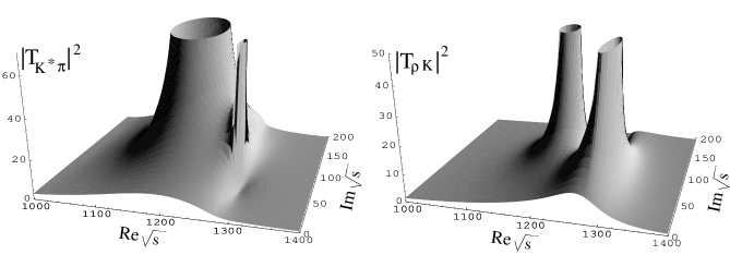
Figure 4: Modulus squared of the amplitudes of Eq. (18) in the unphysical Riemann sheet of the complex $\sqrt{s}$ variable.

In order to see more clearly the contribution of the two $K_{1}(1270)$ poles to the different reactions ($K^{*}\pi$ and $\rho K$), we show in Fig. 4 the modulus squared of the amplitudes of Eq. (18) in the unphysical Riemann sheet of the complex $\sqrt{s}$ variable. The plots have been done with the result of the fit for the $0\leq|t^{\prime}|\leq 0.05$ GeV² data. (The other sets of data give analogous results). The relevant thing for the evaluation of the cross sections of the different reactions is the value of the amplitude in the real axis. We can see very clearly the two different $K_{1}(1270)$ poles and how their different strength and position in the complex plane affects the value in the real axis. For the $K^{*}\pi$ channel we clearly see that the shape in the real axis is essentially determined by the lower mass pole, the higher one having a negligible effect despite being closer to the real axis. For the $\rho K$ case, the shape in the real axis is mainly determined by the higher mass pole. The lower mass pole has a minor influence. In the $\rho K$ case both poles have relevant strength but the fact that the lower mass pole is far away from the real axis makes its effect on it less relevant. It is also worth stressing that the shape of the amplitude in the real axis differs from a Breit-Wigner–like shape.

In a less microscopic approach than the one we do, the $K_{1}(1270)$ could also be parameterized as two explicit Breit-Wigner contributions in order to mimic the two poles building up the $K_{1}(1270)$, similarly as done in Eq. (19) for the $K_{1}(1400)$ with only one Breit-Wigner. However, this procedure requires the knowledge of the couplings to the main channels ($K^{*}\pi$ and $\rho K$), the masses and the widths of the two poles. In this way, one would require four complex parameters for the couplings and four real ones for the masses and widths, instead of just the two complex parameters actually used in Eq. (18) for the $K_{1}(1270)$. Therefore, by removing one global phase, we would be left with 13 free parameters, instead of just the three ones in Eq. (18). This large reduction in the number of free parameters is a remarkable advantage of employing U$\chi$PT in order to describe the two poles that build up the $K_{1}(1270)$. Indeed, as discussed, the data are already well reproduced within our scheme, which explicitly generates the two poles associated with the $K_{1}(1270)$ Roca:2005nm , and adding 10 more free parameters would certainly obscure any possible conclusion. Apart from that, the amplitudes in Eq. (18) also contain non-resonant contributions, beyond what would be obtained by simply taking two Breit-Wigner poles so as to give the amplitudes. In addition, the reproduction of the WA3 data poses an intriguing test to the amplitudes of Ref. Roca:2005nm , which is one of our main aims as well.

IV K-matrix approach

Since the PDG data are largely based on the WA3 data Daum:1981hb , it seems worthwhile to look more closely at the model employed by C. Daum et al. to derive $K_{1}(1270)$ and $K_{1}(1400)$ properties Daum:1981hb . A detailed description of the model can be found in Refs. Daum:1981hb ; Daum:1980ay ; Bowler:1976qe ; Bowler:1974th ; Bowler:1975my . Here, we only briefly summarize the relevant formulae. The production amplitudes are given by

$$F=(1-iK\rho)^{-1}P,$$ (23)

where $K$ is a $n\times n$ matrix with $n$ the number of channels taken into account. In Eq. (23), $\rho$ is a diagonal matrix consisting of phase space and its elements are

$$\rho(s)_{ij}=\frac{p_{i}}{8\pi\sqrt{s}}\delta_{ij}.$$ (24)

The $K$ matrix element is of the following form:

$$K_{ij}=\frac{f_{ai}f_{aj}}{M_{a}-M}+\frac{f_{bi}f_{bj}}{M_{b}-M},$$ (25)

where the decay couplings $f_{ai}$ and $f_{bi}$ are assumed to be real numbers. The production vector $P$ consists of the Deck amplitudes $D$ and the direct production terms $R$

$$P=(1+\alpha K)D+R.$$ (26)

The Deck amplitudes $D$ are parameterized by

$$D_{i}=D_{i0}e^{i\phi_{i}}/(M^{2}_{K\pi\pi}-M^{2}_{K})$$ (27)

and $R$ by

$$R_{i}=\frac{f_{pa}f_{ai}}{M_{a}-M}+\frac{f_{pb}f_{bi}}{M_{b}-M},$$ (28)

where the production couplings $f_{pa}$ and $f_{pb}$ are complex numbers Daum:1981hb ; Daum:1980ay . Furthermore, one can assume $f_{pa}$ to be real. For the constant $\alpha$, a value of $0.4$ was used in Ref. Daum:1981hb . The authors commented that the final results do not depend sensitively on this value. As we will see below, this might not be the case.

Five channels have been included in the ACCMOR analysis Daum:1981hb . For the sake of simplicity, as in other similar theoretical analyses Carnegie:1976cs ; Bowler:1976qe , we have used only two channels, i.e. $K^{*}\pi$ and $\rho K$, which are the most relevant in the analysis of Ref. Daum:1981hb . In this case, there are 13 free parameters: 4 for decay couplings, 3 for production couplings, 4 for Deck backgrounds, and 2 for K-matrix poles $M_{a}$ and $M_{b}$. When this model is used to study the high $|t^{\prime}|$ WA3 data, the following assumption is used, i.e. the decay couplings are the same for $1^{+}S0^{+}$ and $1^{+}S1^{+}$ data, but the production couplings and Deck backgrounds can be different. Therefore, for high $|t^{\prime}|$ data, there are 20 free parameters.

Figure 5: The WA3 data in contrast with the K-matrix approach fit with $M_{a}=1400$ MeV, $M_{b}=1170$ MeV and $\alpha=0.4$.

In our fit of the WA3 data, we fix $M_{a}$ at 1400 MeV and $M_{b}$ at 1170 MeV following the ACCMOR analysis Daum:1981hb . Thus, for low $|t^{\prime}|$ data, we have 11 free parameters and for high $|t^{\prime}|$ data, we have 18 parameters. The obtained results are contrasted with the WA3 data in Fig. 5. It is seen that the agreement is remarkably good. However, one should keep in mind the following: (i) Compared to our model, one has more freedoms in the K-matrix approach. (ii) Although the fit using the K-matrix approach is quantitatively better than our method, the fits are qualitatively very similar.

Figure 6: The same as Fig. 5, but with the contribution of the components of the production amplitude $F$ plotted.

Now, we would like to study the contributions of the components of the production amplitudes $F$ of Eq. (23). In particular, we want to understand the contribution of Deck backgrounds. In Fig. 6, we plot the following quantities $|T_{i}|^{2}q$ with $T_{i}$ being one of the following:

$$T_{1} = (1-iK\rho)^{-1}((1+\alpha K)D+R)\quad\mbox{the full amplitude}$$

$$T_{2} = (1-iK\rho)^{-1}D\quad\mbox{the unitarized Deck background}$$

$$T_{3} = (1-iK\rho)^{-1}(1+\alpha K)D\quad\mbox{the full background}$$

$$T_{4} = (1-iK\rho)^{-1}R\quad\mbox{the direct production amplitude}$$

$$T_{5} = D\quad\mbox{the pure Deck background}$$

From Fig. 6, it is seen that only $T_{3}$ and $T_{4}$ have relevant contributions to the total amplitude. These are the full background and the direct production terms. Surprisingly, the total amplitude seems to originate from the cancellation of two extremely large components: the background and the direct production. In the $K^{*}\pi$ low $|t^{\prime}|$ data, both the background and the direct production amplitudes show no sign of a peak at the experimental lower peak position. Therefore, the lower peak shown in the total amplitude is completely due to the delicate interference between these two large components. Such large destructive interferences seem to be rather artificial, particularly when compared to our fits, where each peak corresponds to a resonance structure. In this sense, our interpretation of the $K_{1}(1270)$ as two poles seems to be favoured, a priori, over the just discussed K-matrix approach, although more data should be compared to reach a definitive, physically sound, statement on this.

In the above fit, we have fixed $\alpha$ at 0.4, the value used by the ACCMOR collaboration Daum:1981hb . In Ref. Daum:1981hb , it was mentioned that the fitted results do not depend sensitively on the value of $\alpha$. We, therefore, have refitted the data by taking $\alpha$ as 0.2 and 0.0. It was found that with smaller $\alpha$, the results obtained are still far away from a straightforward interpretation but less extreme than the case with $\alpha=0.4$. But even if we take $\alpha$ to be zero, the whole amplitude seems to be a result of a delicate interference between the background and the direct production amplitude. Thus, this seems to indicate that the predictions of the K-matrix approach are not very stable. Furthermore, the results with this approach do not stand a clean physical interpretation. We have also refitted the data by setting $M_{b}$ at 1230 MeV and 1270 MeV. The results are in general similar to those with $M_{b}=1170$ MeV. The only difference is that for the $M_{b}=1270$ MeV case, the peak of the high $|t^{\prime}|$ $K^{*}\pi$ results appear 20 MeV higher than the data, thus $M_{b}=1270$ MeV seems to be excluded.

V Contribution of other channels

In our empirical model we constructed above to analyze the WA3 data, we have only included two channels, i.e. $K^{*}\pi$ and $\rho K$. They are the most important channels as can be clearly seen from Figs. 1 and 2. On the other hand, since in our chiral unitary approach, we have three extra channels: $\phi K$, $\omega K$ and $K^{*}\eta$, it would be interesting to show explicitly that their inclusion does not significantly modify our analysis and conclusion. Of course, to include more channels implies, in principle, more free parameters. To overcome this drawback, we turn to SU(3) relations. Supposing that $K_{1}(1270)$ has octet quantum numbers of flavor, its couplings to different channels can be obtained through the following interaction Lagrangian:

$$\mathcal{L}=D\langle\{\phi,V\}S\rangle+F\langle[\phi,V]T\rangle,$$ (29)

where $\phi$ is the pseudoscalar nonet, $V$ the vector octet, and $T$ and $S$ are the octets with positive and negative charge conjugation, respectively. Then the couplings to different channels can be obtained as:

$$g_{K^{*}\pi}=\langle R|\tilde{t}|K^{*}\pi\rangle = \sqrt{\frac{3}{2}}(D+F)$$

$$g_{\rho K}=\langle R|\tilde{t}|\rho K\rangle = -\sqrt{\frac{3}{2}}(D-F)$$

$$g_{K^{*}\eta}=\langle R|\tilde{t}|K^{*}\eta\rangle = \frac{1}{\sqrt{6}}(D-3F)$$

$$g_{\omega K}=\langle R|\tilde{t}|\omega K\rangle = -\frac{1}{\sqrt{2}}(D-F)$$

$$g_{\phi K}=\langle R|\tilde{t}|\phi K\rangle = -(D+F)$$ (30)

We remark that the Lagrangian Eq. (29) follows from just flavour SU(3) symmetry, without invoking any chiral symmetry. Indeed, the relations in Eq. (30) can also be obtained by simply applying the Wigner-Eckert theorem for SU(3) Georgi . Of course, one should expect flavour SU(3) violations in the couplings, but since they are expected to be moderate, and the addition of the extra channels just gives rise to small corrections, these violations would have a very small effect in our fits.

Our total production amplitudes for $K^{*}\pi$ and $\rho K$ are then

$$T_{K^{*}\pi}\equiv T_{\bar{K}^{*0}\pi^{-}} = \sqrt{\frac{2}{3}}g_{K^{*}\pi}+\sqrt{\frac{2}{3}}g_{\phi K}G_{\phi K}t_{\phi K\rightarrow K^{*}\pi}+\sqrt{\frac{2}{3}}g_{\omega K}G_{\omega K}t_{\omega K\rightarrow K^{*}\pi}+\sqrt{\frac{2}{3}}g_{\rho K}G_{\rho K}t_{\rho K\rightarrow K^{*}\pi}$$ (31)

$$+\sqrt{\frac{2}{3}}g_{K^{*}\eta}G_{K^{*}\eta}t_{K^{*}\eta\rightarrow K^{*}\pi}+\sqrt{\frac{2}{3}}g_{K^{*}\pi}G_{K^{*}\pi}t_{K^{*}\pi\rightarrow K^{*}\pi}+\frac{\sqrt{\frac{2}{3}}g^{\prime}_{K^{*}\pi}}{s-M^{2}+iM\Gamma(s)},$$

$$T_{\rho K}\equiv T_{\rho^{0}K^{-}} = -\sqrt{\frac{1}{3}}g_{\rho K}-\sqrt{\frac{1}{3}}g_{\phi K}G_{\phi K}t_{\phi K\rightarrow\rho K}-\sqrt{\frac{1}{3}}g_{\omega K}G_{\omega K}t_{\omega K\rightarrow\rho K}-\sqrt{\frac{1}{3}}g_{\rho K}G_{\rho K}t_{\rho K\rightarrow\rho K}$$ (32)

$$-\sqrt{\frac{1}{3}}g_{K^{*}\eta}G_{K^{*}\eta}t_{K^{*}\eta\rightarrow\rho K}-\sqrt{\frac{1}{3}}g_{K^{*}\pi}G_{K^{*}\pi}t_{K^{*}\pi\rightarrow\rho K}-\frac{\sqrt{\frac{1}{3}}g^{\prime}_{\rho K}}{s-M^{2}+iM\Gamma(s)},$$

where $g^{\prime}_{K^{*}\pi}=\sqrt{\frac{3}{2}}(D^{\prime}+F^{\prime})$ and $g^{\prime}_{\rho K}=\sqrt{\frac{3}{2}}(F^{\prime}-D^{\prime})$ are the couplings of $K_{1}(1400)$ to the $K^{*}\pi$ and $\rho K$ channels by using the same SU(3) symmetry arguments for the $K_{1}(1400)$ resonance. The Clebsch-Gordan coefficient $\sqrt{\frac{2}{3}}$($-\sqrt{\frac{1}{3}}$) again accounts for isospin projection. It is also worth stressing that if the previous equation is particularized to the case of only two channels, $K^{*}\pi$ and $\rho K$, it would be equivalent to Eq. (19).

Using these relations, we have refitted the WA3 data by assuming $D$ real, $F$ complex, $D^{\prime}$ and $F^{\prime}$ complex, given the arbitrariness of a global phase. The results are shown in Fig. 7.

Figure 7: The same as Fig. 3, but the theoretical fit is obtained by including all the five channels: $\phi K$, $\omega K$, $\rho K$, $K^{*}\eta$ and $K^{*}\pi$.

It is seen that they in general resemble those obtained with two channels. The difference is mostly seen in the contribution of $K_{1}(1400)$ in different channels. This can be easily understood because the $K^{*}\eta$, $\omega K$, $\phi K$ channels start to contribute at higher energies and thus distort the $K_{1}(1400)$ contribution seen in Fig. 3. The above analysis showed that (i) The most important channels are $K^{*}\pi$ and $\rho K$. (ii) The SU(3) relations assume that the production vertices are due to pure octet operators. Nevertheless, we find this assumption quite reliable since the $K_{1}$’s resonances of the quark model are SU(3) octets. (iii) The analysis must be understood as providing support for our findings and conclusions with only the two channels $K^{*}\pi$ and $\rho K$.

VI Summary and conclusion

In the present work, we have made a theoretical study of the possible experimental manifestation of the double pole structure of the $K_{1}(1270)$, predicted in a previous work using the techniques of the chiral unitary approach to implement unitarity in the vector-pseudoscalar meson interaction. The model obtains two poles in the $I=1/2$, $S=1$, vector-pseudoscalar scattering amplitudes which can be assigned to two $K_{1}(1270)$ resonances. One pole is at $\sim 1200$ MeV with a width of $\sim 250$ MeV and the other is at $\sim 1280$ MeV with a width of $\sim 150$ MeV. The lower pole couples more to the $K^{*}\pi$ channel and the higher pole couples dominantly to the $\rho K$ channel. Different reaction mechanisms may prefer different channels and thus this explains the different invariant mass distributions seen in various experiments. We have analyzed the WA3 data on the $K^{-}p\to K^{-}\pi^{+}\pi^{-}p$ reaction since it is the most conclusive and high-statistics experiment quoted in the PDG on the $K_{1}(1270)$ resonance. Our model obtains a good description of the WA3 data both for the $K^{*}\pi$ and $\rho K$ final state channels. In our model, the peak in the $K\pi\pi$ mass distribution around the $1270$ MeV region is a superposition of the two poles, but in the $K^{*}\pi$ channel the lower pole dominates and in the $\rho K$ channel the higher pole gives the biggest contribution. It is worth stressing that the physical properties quoted in the PDG obtained from the WA3 data analysis rely, obviously, upon considering only one pole for the $K_{1}(1270)$. These data have long been interpreted by assuming either a substantial Gaussian background or unitarized Deck background. While the Gaussian background method is purely empirical, we have shown that the Deck background method seems to suffer from instability and critical destructive interferences. In contrast, and as we mentioned above, the data can be explained in simpler terms by our model, where every peak corresponds to resonances. Of course, this fact, although desirable, is not a physical requirement and more data should be analyzed to finally distinguish between our proposal, with two poles making up the $K_{1}(1270)$ resonance, and that with only one pole.

On the other hand, it is worth mentioning that in the literature, the $K_{1}(1270)$ and the $K_{1}(1400)$ resonances have always been considered as a mixture of the two corresponding SU(3) eigenstates. The mixing is defined by a mixing angle $\theta_{K}$. The value of this angle has been under extensive study for many years but no consensus has yet been reached. Recent studies seem to favor a value of $\sim 60\hbox{${}^{\circ}$}$ (see Refs. Roca:2003uk ; Li:2006we for a short review). An interesting issue, however, has been raised by the BES study of charmonium decays to axial-vector plus pseudoscalar mesons. In $\psi(2s)$ decay, they found the $\psi(2s)\rightarrow K_{1}(1400)\bar{K}$ branching fraction is smaller than that for the $\psi(2s)\rightarrow K_{1}(1270)\bar{K}$ by at least a factor of 3. To accommodate this, one needs a mixing angle of $\theta_{K}<29\hbox{${}^{\circ}$}$. While in the $J/\psi$ decay, the $J/\psi\rightarrow K_{1}(1400)\bar{K}$ branching fraction is larger than the upper limit for the $J/\psi\rightarrow K_{1}(1270)\bar{K}$ mode. This would require a mixing angle of $\theta_{K}>48\hbox{${}^{\circ}$}$. As a possible future application of our framework, these two different values for the mixing angle could be possibly explained if one assumes that in the $\psi(2s)$ and $J/\psi$ decays, one actually sees the different two poles of the $K_{1}(1270)$ that we are referring in this work. As the two poles would mix differently with the $K_{1}(1400)$, they would give rise to different values for the mixing angles. In this sense, more high-statistics data of $\psi(2s)$ and $J/\psi$ decay would be very helpful to test the above assumption.

VII Acknowledgments

L. S. Geng acknowledges many useful discussions with Alberto Martínez, Michael Doering, Kanchan Khemchandani and M. J. Vicente Vacas. We would like to thank W. Ford for valuable comments regarding the experiments used in this paper. This work is partly supported by DGICYT Contract No. BFM2003-00856, FPA2004-03470, the Generalitat Valenciana, and the E.U. FLAVIAnet network Contract No. HPRN-CT-2002-00311. This research is part of the EU Integrated Infrastructure Initiative Hadron Physics Project under Contract No. RII3-CT-2004-506078.

References

- (1) W. M. Yao et al. [Particle Data Group], J. Phys. G 33, 1 (2006).
- (2) J. Z. Bai et al. [BES Collaboration], Phys. Rev. Lett. 83, 1918 (1999) [arXiv:hep-ex/9901022].
- (3) L. Roca, E. Oset and J. Singh, Phys. Rev. D 72, 014002 (2005) [arXiv:hep-ph/0503273].
- (4) V. K. Magas, E. Oset and A. Ramos, Phys. Rev. Lett. 95, 052301 (2005) [arXiv:hep-ph/0503043].
- (5) R. Armenteros et al. Phys. Lett. B 9, 207 (1964).
- (6) A. Astier et al., Nucl. Phys. B 10, 65 (1969).
- (7) A. Firestone, G. Goldhaber, D. Lissauer and G. H. Trilling, Phys. Rev. D 5, 505 (1972).
- (8) P. Gavillet et al. [Amsterdam-CERN-Nijmegen-Oxford Collaboration], Phys. Lett. B 76, 517 (1978).
- (9) S. Rodeback et al. [CERN-College de France-Madrid-Stockholm Collaboration], Z. Phys. C 9, 9 (1981).
- (10) G. W. Brandenburg et al., Phys. Rev. Lett. 36, 703 (1976).
- (11) C. Daum et al. [ACCMOR Collaboration], Nucl. Phys. B 187, 1 (1981).
- (12) K. Abe et al. [Belle Collaboration], Phys. Rev. Lett. 87, 161601 (2001) [arXiv:hep-ex/0105014].
- (13) D. M. Asner et al. [CLEO Collaboration], Phys. Rev. D 62, 072006 (2000) [arXiv:hep-ex/0004002].
- (14) D. V. Bugg, Eur. Phys. J. A 25, 107 (2005) [Erratum-ibid. A 26, 151 (2005)] [arXiv:hep-ex/0510026].
- (15) M. Ablikim et al. [BES Collaboration], Phys. Lett. B 633, 681 (2006) [arXiv:hep-ex/0506055].
- (16) G. Otter et al. [Aachen-Berlin-CERN-London-Vienna Collaboration], Nucl. Phys. B 106, 77 (1976).
- (17) J. S. M. Vergeest et al. [AMSTERDAM-CERN-NIJMEGEN-OXFORD Collaboration], Nucl. Phys. B 158, 265 (1979).
- (18) M. G. Bowler, J. Phys. G 3, 775 (1977).
- (19) S. Weinberg, PhysicaA 96, 327 (1979).
- (20) J. Gasser and H. Leutwyler, Nucl. Phys. B 250, 465 (1985).
- (21) U. G. Meissner, Rept. Prog. Phys. 56, 903 (1993) [arXiv:hep-ph/9302247].
- (22) V. Bernard, N. Kaiser and U. G. Meissner, Int. J. Mod. Phys. E 4, 193 (1995) [arXiv:hep-ph/9501384].
- (23) A. Pich, Rept. Prog. Phys. 58, 563 (1995) [arXiv:hep-ph/9502366].
- (24) G. Ecker, Prog. Part. Nucl. Phys. 35, 1 (1995) [arXiv:hep-ph/9501357].
- (25) M. F. M. Lutz and E. E. Kolomeitsev, Nucl. Phys. A 730, 392 (2004) [arXiv:nucl-th/0307039].
- (26) A. Dobado and J. R. Pelaez, Phys. Rev. D 56, 3057 (1997) [arXiv:hep-ph/9604416].
- (27) J. A. Oller, E. Oset and J. R. Pelaez, Phys. Rev. Lett. 80, 3452 (1998) [arXiv:hep-ph/9803242].
- (28) J. A. Oller, E. Oset and J. R. Pelaez, Phys. Rev. D 59, 074001 (1999) [Erratum-ibid. D 60, 099906 (1999)] [arXiv:hep-ph/9804209].
- (29) J. A. Oller and E. Oset, Phys. Rev. D 60, 074023 (1999) [arXiv:hep-ph/9809337].
- (30) J. A. Oller and E. Oset, Nucl. Phys. A 620, 438 (1997) [Erratum-ibid. A 652, 407 (1999)] [arXiv:hep-ph/9702314].
- (31) M. C. Birse, Z. Phys. A 355, 231 (1996) [arXiv:hep-ph/9603251].
- (32) S. M. Flatte, Phys. Lett. B 63, 224 (1976).
- (33) R. K. Carnegie, R. J. Cashmore, M. Davier, W. M. Dunwoodie, T. A. Lasinski, D. W. G. Leith and S. H. Williams, Nucl. Phys. B 127, 509 (1977).
- (34) C. Daum et al. [ACCMOR Collaboration], Nucl. Phys. B 182, 269 (1981).
- (35) M. G. Bowler, J. B. Dainton, A. Kaddoura and I. J. R. Aitchison, Nucl. Phys. B 74, 493 (1974).
- (36) M. G. Bowler, M. A. V. Game, I. J. R. Aitchison and J. B. Dainton, Nucl. Phys. B 97, 227 (1975).
- (37) H. Georgi, Lie Algebras in Particle Physics, (Westview Press, Colorado, 1999), 2nd ed.
- (38) L. Roca, J. E. Palomar and E. Oset, Phys. Rev. D 70, 094006 (2004) [arXiv:hep-ph/0306188].
- (39) D. M. Li and Z. Li, Eur. Phys. J. A 28, 369 (2006) [arXiv:hep-ph/0606297].