Bounds on length scales of classical spacetime foam models

Abstract

Simple models of a classical spacetime foam are considered, which consist of identical static defects embedded in Minkowski spacetime. Plane-wave solutions of the vacuum Maxwell equations with appropriate boundary conditions at the defect surfaces are obtained in the long-wavelength limit. The corresponding dispersion relations $\omega^{2}=\omega^{2}(\vec{k})$ are calculated, in particular, the coefficients of the quadratic and quartic terms in $\vec{k}$. Astronomical observations of gamma–ray bursts and ultra-high-energy cosmic rays then place bounds on the coefficients of the dispersion relations and, thereby, on particular combinations of the fundamental length scales of the static spacetime-foam models considered. Spacetime foam models with a single length scale are excluded, even models with a length scale close to the Planck length (as long as a classical spacetime remains relevant).

I Introduction

Whether or not space remains smooth down to smaller and smaller distances is an open question. Conservatively, one can say that the typical length scale of any fine-scale structure of space must be less than $10^{-18}\,\text{m}=10^{-3}\,\text{fm}$, which corresponds to the inverse of a center-of-mass energy of $200\,\text{GeV}$ in a particle-collider experiment. Astrophysics provides us, of course, with much higher energies, but not with controllable experiments. Still, astrophysics may supply valuable information as long as the relevant physics is well understood.

In this article, we discuss astrophysical bounds solely based on solutions of the Maxwell (and Dirac) equations. These solutions hold for a particular type of classical spacetime with nontrivial small-scale structure. Specifically, we consider a static (time-independent) fine-scale structure of space, which is modeled by a homogeneous and isotropic distribution of identical static “defects” embedded in Minkowski spacetime. With appropriate boundary conditions at the defect surfaces, plane-wave solutions of the vacuum Maxwell equations are obtained in the long-wavelength limit. That is, the wavelength $\lambda$ must be much larger than $\max(b,l)$, with $b$ the typical size of the individual defect and $l$ the mean separation between the different defects. An (imperfect) analogy would be sound propagation in a block of ice with frozen-in bubbles of air.

Generalizing the terminology of Wheeler and Hawking W57 ; W68 ; H78 ; HPP80 ; Fetal90 ; V96 , we call any classical spacetime with nontrivial small-scale structure (resembling bubbly ice, Swiss cheese, or whatever) a “classical spacetime foam.” The plane-wave Maxwell solutions from our classical spacetime-foam models, then, have a modified dispersion relation (angular frequency squared as a function of the wave number $k\equiv|\vec{k}|\equiv 2\pi/\lambda$):

$$\omega^{2}_{\gamma}\,\Big{|}^{[\text{defect type}\,\tau]} = a_{\gamma\,2}^{[\tau]}\;\,c^{2}\,k^{2}+a_{\gamma\,4}^{[\tau]}\;\big{(}\,b^{[\tau]}\,\big{)}^{2}\,c^{2}\,k^{4}+\ldots\,,$$ (1)

where $c$ is the characteristic velocity of the Minkowski line element ($\text{d}s^{2}=c^{2}\,\text{d}t^{2}-|\text{d}\vec{x}|^{2}$ ), $a_{\gamma\,2}$ and $a_{\gamma\,4}$ are dimensionless coefficients depending on the fundamental length scales of the model (one length scale being $b$), and $\tau$ labels different kinds of models.

For simplicity, we consider only three types of static defects (or “weaving errors” in the fabric of space):

1. a nearly pointlike defect with the interior of a ball removed from $\mathbb{R}^{3}$ and antipodal points on its boundary identified;

2. a nearly pointlike defect with the interior of a ball removed from $\mathbb{R}^{3}$ and boundary points reflected in an equatorial plane identified;

3. a wormhole-like defect with two balls removed from $\mathbb{R}^{3}$ and glued together on their boundaries; cf. Refs. Fetal90 ; V96 .

Further details will be given in Sec. II.1. As mentioned above, the particular spacetime models considered consist of a frozen gas of identical defects (types $\tau=1$, $2$, $3$) distributed homogeneously and isotropically over Euclidean space $\mathbb{R}^{3}$. We emphasize that these classical models are not intended to describe in any detail a possible spacetime-foam structure (which is, most likely, essentially quantum-mechanical in nature) but are meant to provide simple and clean backgrounds for explicit calculations of potential nonstandard propagation effects of electromagnetic waves.

The type of Maxwell solution found here is reminiscent of the solution from the so-called “Bethe holes” for waveguides B44 . In both cases, the standard Maxwell plane wave is modified by the radiation from fictitious multipoles located in the holes or defects. But there is a crucial difference: for Bethe, the holes are in a material conductor, whereas for us, the defects are “holes” in space itself.

Returning to our spacetime-foam models, we also calculate the modified dispersion relation of a free Dirac particle, for definiteness taken to be a proton (mass $m_{p}$):

$$\omega^{2}_{p}\,\Big{|}^{[\text{defect type}\,\tau]}=a_{p\,0}^{[\tau]}\;\,\hbar^{-2}\,c^{4}\,m_{p}^{2}+a_{p\,2}^{[\tau]}\;\,c^{2}\,k^{2}+a_{p\,4}^{[\tau]}\;\big{(}\,b^{[\tau]}\,\big{)}^{2}\,c^{2}\,k^{4}+\ldots\,,$$ (2)

with reduced Planck constant $\hbar\equiv h/2\pi$ and dimensionless coefficients $a_{p\,0}$, $a_{p\,2}$, and $a_{p\,4}\,$. As might be expected, the response of Dirac and Maxwell plane waves to the same spacetime-foam model turns out to be quite different, with unequal quadratic coefficients $a_{p\,2}$ and $a_{\gamma\,2}$, for example. The different proton and photon velocities then allow for Cherenkov–type processes Beall1970 ; ColemanGlashow1997 . But, also in the pure photon sector, there can be interesting time-dispersion effects AEMNS98 as long as the quartic coefficient $a_{\gamma\,4}$ of the photon dispersion relation (1) is nonvanishing.

In fact, with the model dispersion relations in place, we may use astronomical observations to put bounds on the various coefficients $a_{2}$ and $a_{4}$, and, hence, on particular combinations of the model length scales (e.g., average defect size $\overline{b}$ and separation $\overline{l}\,$). Specifically, the absence of time dispersion in an observed TeV flare from an active galactic nucleus bounds $|a_{\gamma\,4}|$ and the absence of Cherenkov–like effects in ultra-high-energy cosmic rays bounds $(a_{\gamma\,2}-a_{p\,2})$ and $a_{\gamma\,4}$. In other words, astrophysics not only explores the largest structures of space (up to the size of the visible universe at approximately $10^{10}\,\text{lyr}\approx 10^{26}\,\text{m}$) but also the smallest structures (down to $10^{-26}\,\text{m}$ or less, as will be shown later on).

The outline of the remainder of this article is as follows. In Sec. II, we discuss the calculation of the effective photon dispersion relation from the simplest type of foam model, with static $\tau=1$ defects. The calculations for isotropic $\tau=2$ and $\tau=3$ models are similar and are not discussed in detail (App. A gives additional results for anisotropic defect distributions). Some indications are, however, given for the calculation of the proton dispersion relation from model $\tau=1$ with details relegated to App. B. The main focus of Sec. II and the two appendices is on modified dispersion relations but in Sec. II.3 we also discuss the Rayleigh-like scattering of an incoming electromagnetic wave by the model defects. In Sec. III, we summarize the different dispersion relations calculated and put the results in a general form. In Sec. IV, this general photon dispersion relation is confronted to the astronomical observations and bounds on the effective length scales are obtained. In Sec. V, we draw an important conclusion for the classical small-scale structure of space and present some speculations on a hypothetical quantum spacetime foam.

II Calculation

II.1 Defect types

The present article considers three types of static defects obtained by surgery on the Euclidean 3–space $\mathbb{R}^{3}$. The discussion is simplified by initially choosing the origin of the Cartesian coordinates $\vec{x}\equiv(x^{1},x^{2},x^{3})\equiv(x,y,z)$ of $\mathbb{R}^{3}$ to coincide with the “center” of the defect. The corresponding Minkowski spacetime $\mathbb{R}\times\mathbb{R}^{3}$ has standard metric $(\eta_{\mu\nu})=\text{diag}(1,-1,-1,-1)$ for coordinates $x^{\mu}=(x^{0},\vec{x})=(c\,t,x^{m})$ with index $\mu=0$, $1$, $2$, $3$.

The first type of defect (label $\tau=1$) is obtained by removing the interior of a ball from $\mathbb{R}^{3}$ and identifying antipodal points on its boundary. Denote this ball, its boundary sphere, and point reflection by

$$B_{b} = \big{\{}\vec{x}\in\mathbb{R}^{3}:\,|\vec{x}|\leq b\big{\}}\,,\quad$$ (3a)

$$S_{b} = \big{\{}\vec{x}\in\mathbb{R}^{3}:\,|\vec{x}|=b\big{\}}\,,\quad$$ (3b)

$$P(\vec{x}) = -\vec{x}\,.$$ (3c)

Then, the 3–space with a single defect centered at the origin $\vec{x}=0$ is given by

$$\mathsf{M}^{[\tau=1]}_{b}\equiv\mathsf{M}^{[\tau=1]}_{0,\,b}=\big{\{}\vec{x}\in\mathbb{R}^{3}:\,|\vec{x}|\geq b\,\wedge\,\left(S_{b}\ni\vec{x}\;\cong\;P(\vec{x})\in S_{b}\right)\big{\}}\,,$$ (4)

where $\cong$ denotes pointwise identification and $\mathsf{M}^{[\tau=1]}_{b}$ is a shorthand notation. The 3–space (4) has no boundary because of the $S_{b}$ identifications (cf. Figure 1) and, away from the defect at $|\vec{x}|=b$, is certainly a manifold (hence, the suggestive notation $\mathsf{M}$). The resulting spacetime is $\mathcal{M}=\mathbb{R}\times\mathsf{M}^{[\tau=1]}_{b}\,$.

The corresponding classical spacetime-foam model is obtained from a superposition of $\tau=1$ defects with a homogeneous distribution. The number density of defects is denoted $n\equiv l^{-3}$ and only the case of a very rarefied gas of defects is considered ($b\ll l$), so that there is no overlap of defects. Clearly, there is a preferred reference frame for which the defects are static. Such a preferred frame, in the context of cosmology, may or may not be related to the preferred frame of the isotropic cosmic microwave background.

In more detail, the construction is as follows. The 3–space with $N\geq 1$ identical defects is given by

$$\mathsf{M}^{[\tau=1]}_{\{\vec{x}_{1},\,\ldots,\,\vec{x}_{N}\},\,b}=\mathsf{M}^{[\tau=1]}_{\vec{x}_{1},\,b}\cap\mathsf{M}^{[\tau=1]}_{\vec{x}_{2},\,b}\cap\ldots\cap\mathsf{M}^{[\tau=1]}_{\vec{x}_{N},\,b}\;,$$ (5)

where $\mathsf{M}^{[\tau=1]}_{\vec{x}_{n},\,b}$ is the single-defect 3–space (4) with the center of the sphere moved from $\vec{x}=0$ to $\vec{x}=\vec{x}_{n}$. The minimum distance between the different centers $\vec{x}_{n}$ of 3–space (5) is assumed to be larger than $2b$. The final spacetime foam model results from taking the Cartesian product of $\mathbb{R}$ with the $N\to\infty$ “limit” of (5),

$$\mathcal{M}^{[\tau=1]}_{\text{distribution},\,b}=\mathbb{R}\times\left(\,\lim_{N\to\infty}\mathsf{M}^{[\tau=1]}_{\{\vec{x}_{1},\,\ldots,\,\vec{x}_{N}\},\,b}\,\right)\,,$$ (6)

where one needs to give the statistical distribution of the centers $\vec{x}_{n}$. As mentioned above, we choose the simplest possible distribution, homogeneous, and the quantity to specify is the number density $n$ of defects.

The second type of defect ($\tau=2$) follows by the same construction, except that the identified points of the sphere $S_{b}$ are obtained by reflection in an equatorial plane with unit normal vector $\widehat{a}$. For a point $\vec{x}$ on the sphere $S_{b}$, the reflected point is denoted $R_{\widehat{a}}(\vec{x})$. [With only one defect present, global Cartesian coordinates can be chosen so that $\widehat{a}$ points in the 3–direction and $(x^{1},x^{2},x^{3})\in S_{b}$ is to be identified with $(x^{1},x^{2},-x^{3})\in S_{b}$.] The space with a single $\tau=2$ defect centered at the origin $\vec{x}=0$ (not indicated by our shorthand notation) is then given by (cf. Figure 2)

$$\mathsf{M}^{[\tau=2]}_{\widehat{a},\,b}=\big{\{}\vec{x}\in\mathbb{R}^{3}:\,|\vec{x}|\geq b\,\wedge\,\left(S_{b}\ni\vec{x}\;\cong\;R_{\widehat{a}}(\vec{x})\in S_{b}\right)\big{\}}\,,$$ (7)

and spacetime is $\mathbb{R}\times\mathsf{M}^{[\tau=2]}_{\widehat{a},\,b}$. However, the defect embedded in (7) is not a manifold but an orbifold Nakahara90 , i.e., a coset space $\mathsf{M}/G$, for manifold $\mathsf{M}$ and discrete symmetry group $G$. The 3–space (7) has, in fact, singular points corresponding to the fixed points of $R_{\widehat{a}}$, which lie on the great circle of $S_{b}$ in the equatorial plane with normal vector $\widehat{a}$. But away from these singular points, the 3–space is a genuine manifold and we simply use the (slightly misleading) notation $\mathsf{M}$ in (7). The corresponding classical spacetime-foam model results from a homogeneous and isotropic (randomly oriented) distribution of $\tau=2$ defects.

The third type of defect ($\tau=3$) is obtained by a somewhat more extensive surgery Fetal90 ; V96 . Now, the interiors of two identical balls are removed from $\mathbb{R}^{3}$. These balls, denoted $B_{b}$ and $B_{b}^{\prime}$, have their centers separated by a distance $d>2b$. The two boundary spheres $S_{b}$ and $S_{b}^{\prime}$ are then pointwise identified by reflection in the central plane. This reflection is again denoted $R_{\widehat{a}}$. [With ball centers at $\vec{x}=(\pm d/2,0,0)$, the reflection plane is given by $x^{1}=0$.] The space manifold with a single $\tau=3$ defect centered at the origin $\vec{x}=0$ is now (cf. Figure 3)

$$\mathsf{M}^{[\tau=3]}_{\widehat{a},b,d}=\big{\{}\vec{x}\in\mathbb{R}^{3}:\,|\vec{x}-(d/2)\,\widehat{a}\,|\geq b\,\wedge\,|\vec{x}+(d/2)\,\widehat{a}\,|\geq b\,\wedge\,\left(S_{b}\ni\vec{x}\;\cong\;R_{\widehat{a}}(\vec{x})\in S_{b}^{\prime}\,\right)\big{\}}\,,$$ (8)

and the spacetime manifold is $\mathbb{R}\times\mathsf{M}^{[\tau=3]}_{\widehat{a},b,d}$. Using standard wormhole terminology W57 ; W68 ; H78 ; HPP80 ; Fetal90 ; V96 , the static $\tau=3$ defect has two “wormhole mouths” of diameter $2b$, with corresponding points on the wormhole mouths separated by a vanishing distance through the “wormhole throat” and by a “long distance” $D\in[d-2b,d+\pi b]$ via the ambient Euclidean space. Again, the corresponding classical spacetime-foam model results from a homogeneous and isotropic distribution of $\tau=3$ defects.

For later use, we also define a $\tau=3^{\prime}$ defect with distance $d$ set to the value $4b$, where the factor $4$ has been chosen arbitrarily. An individual $\tau=3^{\prime}$ defect then has only one length scale, $b$, which simplifies some of the discussion later on. The relevant space manifold is thus

$$\mathsf{M}^{[\tau=3^{\prime}]}_{\widehat{a},\,b}\equiv\mathsf{M}^{[\tau=3]}_{\widehat{a},b,4b}\;,$$ (9)

in terms of the $\tau=3$ manifold defined by (8).

Let us end this subsection with two parenthetical remarks, one mathematical and one physical. First, the $\tau=1$ and $\tau=3$ spaces are multiply connected (i.e., have noncontractible loops) but not the $\tau=2$ space. Second, the classical spacetimes considered in this article do not solve the vacuum Einstein equations but appear to require some exotic form of energy located at the defects; see, e.g., Part III of Ref. V96 for further discussion. In one way or another, the fine-scale structure of spacetime may very well be related to the “dark energy” of cosmology; see, e.g. Refs. PeeblesRatra2002 ; Spergel-etal2006 and references therein.

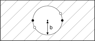
Figure 1: Three-space (4) from a single spherical defect (type $\tau=1$, radius $b$) embedded in $\mathbb{R}^{3}$, with its “interior” removed and antipodal points identified (as indicated by the pairs of open and filled circles). The corresponding classical spacetime-foam model has a homogeneous distribution of static $\tau=1$ defects embedded in Minkowski spacetime.

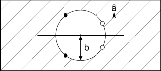
Figure 2: Three-space (7) from a single spherical defect (type $\tau=2$, radius $b$) embedded in $\mathbb{R}^{3}$, with its “interior” removed and points identified by reflection in the equatorial plane with normal vector $\widehat{a}$. The corresponding classical spacetime-foam model has a homogeneous and isotropic distribution of static $\tau=2$ defects embedded in Minkowski spacetime.

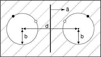
Figure 3: Three-space (8) from a single wormhole-like defect (type $\tau=3$, two spheres with radii $b$ and distance $d$ between the centers) embedded in $\mathbb{R}^{3}$, with the “interiors” of the two spheres removed and their points identified by reflection in the central plane with normal vector $\widehat{a}$. The corresponding classical spacetime-foam model has a homogeneous and isotropic distribution of static $\tau=3$ defects embedded in Minkowski spacetime.

II.2 Photon dispersion relation

The task, now, is to determine the electromagnetic-wave properties for the three types of classical spacetime-foam models considered. The $\tau=1$ case will be discussed in some detail but not the other cases ($\tau=2$, $3$), for which only results will be given.

The calculation is relatively straightforward and consists of three steps. First, recall the vacuum Maxwell equations in Gaussian units PP62 ; F64 ; J75 ,

$$\nabla\cdot\vec{E} = 0\,,\quad c\,\nabla\times\vec{E}+\partial_{t}\vec{B}=0\,,$$ (10a)

$$\nabla\cdot\vec{B} = 0\,,\quad c\,\nabla\times\vec{B}-\partial_{t}\vec{E}=0\,,$$ (10b)

and the standard plane-wave solution over Minkowski spacetime,

$$\vec{E}_{0}(\vec{x},t) = E_{0}\,\widehat{x}\;\exp({\rm i}\,kz-{\rm i}\,\omega_{\gamma}t)\,,$$ (11a)

$$\vec{B}_{0}(\vec{x},t) = E_{0}\,\widehat{y}\;\exp({\rm i}\,kz-{\rm i}\,\omega_{\gamma}t)\,,$$ (11b)

with amplitude $E_{0}$ and dispersion relation $\omega_{\gamma}^{2}=c^{2}\,k^{2}$. This particular solution corresponds to a linearly polarized plane wave propagating in the $z\equiv x^{3}$ direction ($\widehat{x}$ and $\widehat{y}$ are unit vectors pointing in the $x^{1}$ and $x^{2}$ directions, respectively). The pertinent observation, now, is that the electromagnetic fields (11) also provide a valid solution of the Maxwell equations between the “holes” of the classical spacetime-foam models considered, for example, model (6) for $\tau=1$ defects.

Second, add appropriate vacuum solutions ($\vec{E}_{1},\vec{B}_{1}$), so that the total electric and magnetic fields, $\vec{E}=\vec{E}_{0}+\vec{E}_{1}$ and $\vec{B}=\vec{B}_{0}+\vec{B}_{1}$, satisfy the boundary conditions from a single defect. The specific boundary conditions for the electric field at the defect surface follow by considering the allowed motions of an electrically charged test particle and similarly for the boundary conditions of the magnetic field. Geometrically, the electromagnetic-field boundary conditions trace back to the proper identification of the defect surface points and their tangential spaces.

Third, sum over the contributions ($\vec{E}_{j},\vec{B}_{j}$) of the different defects ($j=1$, $2$, $3$, $\ldots$) in the model spacetime foam and obtain the effective dielectric and magnetic permeabilities, $\epsilon$ and $\mu$, which may be wavelength dependent. The dispersion relation for the isotropic case is then given by

$$\omega_{\gamma}^{2}(k)=c^{2}\,k^{2}/\big{(}\epsilon(k)\,\mu(k)\big{)}\,,$$ (12)

and we refer the reader to the textbooks for further discussion (see, e.g., Sec. II–32–3 of Ref. F64 and Secs. 7.5(a) and 9.5(d) of Ref. J75 ).

The specifics of the second and third step of the calculation for $\tau=1$ defects are as follows. In step 2, the motion of a test particle under influence of the Lorentz force (see, for example, the points marked in Fig. 1 for tangential motion) gives the following boundary conditions at the surface $S_{b}$ of 3–space (4):

$$\widehat{n}(\vec{x})\cdot\vec{E}(\vec{x},t) = -\widehat{n}(-\vec{x})\cdot\vec{E}(-\vec{x},t)\,,\;\;\widehat{n}(\vec{x})\times\vec{E}(\vec{x},t)=+\widehat{n}(-\vec{x})\times\vec{E}(-\vec{x},t)\;\Big{|}_{\,|\vec{x}|=b}^{\,[\tau=1]}\,,$$ (13a)

$$\widehat{n}(\vec{x})\cdot\vec{B}(\vec{x},t) = +\widehat{n}(-\vec{x})\cdot\vec{B}(-\vec{x},t)\,,\;\;\widehat{n}(\vec{x})\times\vec{B}(\vec{x},t)=-\widehat{n}(-\vec{x})\times\vec{B}(-\vec{x},t)\;\Big{|}_{\,|\vec{x}|=b}^{\,[\tau=1]}\,,$$ (13b)

where $\widehat{n}(\vec{x})$ is the outward unit normal vector of the surface at point $\vec{x}\in S_{b}\subset\mathbb{R}^{3}$. The boundary conditions (13) also ensure an equal Poynting vector $c(\vec{E}\times\vec{B})/4\pi$ at antipodal points, as might be expected for an energy-flux density passing through the defect. As mentioned above, these boundary conditions trace back to the antipodal identification of the points on the surface $S_{b}$ and the identification of the respective tangential spaces.

Constant fields $\vec{E}\propto E_{0}\,\widehat{x}$ and $\vec{B}\propto E_{0}\,\widehat{y}$, corresponding to the unperturbed fields (11) over distances of order $b\ll\lambda$, do not satisfy the defect boundary conditions (13) and need to be corrected. As discussed in the Introduction, the correction fields $\vec{E}_{1}$ and $\vec{B}_{1}$ correspond to multipole fields from “mirror charges” located inside the defect. The leading contributions of a $\tau=1$ defect come from fictitious electric and magnetic dipoles at the defect center, each aligned with their respective initial fields (11) and both with a strength proportional to $b^{3}\,E_{0}$. For $\tau=1$ and $kb\ll 1$, the electric field $\vec{E}=\vec{E}_{0}+\vec{E}_{1}$ turns out to be normal to the surface $S_{b}$ and the magnetic field $\vec{B}=\vec{B}_{0}+\vec{B}_{1}$ tangential, just as for a perfectly conducting sphere (see, e.g., Secs. 13.1 and 13.9 of Ref. PP62 ).

In step 3 of the calculation for $\tau=1$ defects, the effective dielectric and magnetic permeabilities (Gaussian units) are found to be given by

$$\epsilon^{[\tau=1]} \!\!\sim\!\! 1+4\pi\,nb^{3}\big{[}j_{0}(kb)+j_{2}(kb)\big{]}\,,$$ (14a)

$$\mu^{[\tau=1]} \!\!\sim\!\! 1-2\pi\,nb^{3}\big{[}j_{0}(kb)+j_{2}(kb)\big{]}\,,$$ (14b)

where $n\equiv 1/l^{3}$ is the number density of defects (mean separation $l$) and $j_{p}(z)$ is the spherical Bessel function of order $p$, for example, $j_{0}(z)=(\sin z)/z$. The similarity signs in Eqs. (14a) and (14b) indicate that only the $\ell=1$ multipoles have been taken into account endnote-multipoles . With (12), the dispersion relation is then

$$\Big{(}\omega^{[\tau=1]}_{\gamma}(k)\Big{)}^{2}\sim\frac{c^{2}\,k^{2}}{\big{(}1+4\pi\,nb^{3}\left[j_{0}(kb)+j_{2}(kb)\right]\big{)}\big{(}1-2\pi\,nb^{3}\left[j_{0}(kb)+j_{2}(kb)\right]\big{)}}\;,$$ (15)

which holds for $kb\ll kl\ll 1$. A Taylor expansion in $nb^{3}$ and $kb$ gives

$$\Big{(}\omega^{[\tau=1]}_{\gamma}(k)\Big{)}^{2} \sim \left(1-2\pi\,nb^{3}\right)\,c^{2}\,k^{2}+(\pi/5)\,nb^{5}\,c^{2}\,k^{4}+\ldots\;.$$ (16)

As mentioned already, the dispersion relation (15) has only been derived for sufficiently small values of $k$. However, taking this expression (15) at face value, we note that the corresponding front velocity ($v_{\text{front}}\equiv\lim_{k\to\infty}\,v_{\text{phase}}$) would be precisely $c$. See, e.g., Ref. Brillouin1960 for the relevance of the front velocity to the issues of signal propagation and causality.

For the $\tau=2$ spacetime-foam model, the dispersion relation is found to be given by

$$\Big{(}\omega^{[\tau=2]}_{\gamma}(k)\Big{)}^{2}\sim\frac{c^{2}\,k^{2}}{1+2\pi\,nb^{3}\,\big{[}j_{0}(kb)+j_{2}(kb)\big{]}}\;,$$ (17)

with Taylor expansion

$$\Big{(}\omega^{[\tau=2]}_{\gamma}(k)\Big{)}^{2} \!\!\sim\!\! \left(1-2\pi\,nb^{3}\right)\,c^{2}\,k^{2}+(\pi/5)\,nb^{5}\,c^{2}\,k^{4}+\ldots\,.$$ (18)

Apparently, the result (18) for randomly orientated $\tau=2$ defects agrees, to the order shown, with the previous result (16) for unoriented $\tau=1$ defects. Some results for anisotropic defect distributions are given in App. A.

For the $\tau=3$ spacetime-foam model, the calculation is more complicated as the correction fields of the two “wormhole mouths” [spheres $S_{b}$ and $S_{b}^{\prime}$ in Eq. (8)] affect each other. Therefore, we have to work directly with Taylor expansions in $b/d$. Giving only the leading order terms in $b/d$, the end result is

$$\Big{(}\omega^{[\tau=3]}_{\gamma}(k)\Big{)}^{2} \!\!\sim\!\! \left(1-(20\,\pi/3)\,nb^{3}\right)\,c^{2}\,k^{2}+(2\pi/9)\,nb^{3}\,d^{2}\,c^{2}\,k^{4}+\ldots\,,$$ (19)

which holds for $kb\ll kd\ll kl\ll 1$. For anisotropic defect distributions, some results are again given in App. A.

In closing, it is to be emphasized that any localized defect (weaving error) of space responds to an incoming electromagnetic plane wave by radiation fields corresponding to fictitious multipoles B44 . Only the position and relative strengths of these multipoles depend on the detailed structure of the defect. Together with the statistical distribution of the defects, these details then determine the precise numerical coefficients of the modified photon dispersion relation written as a power series in $\vec{k}$ (see Sec. III for further discussion).

II.3 Scattering

In this subsection, another aspect of electromagnetic-wave propagation is discussed, namely, the scattering of an incoming plane wave by $\tau=1$ defects. Similar results are expected for $\tau=2$ and $\tau=3^{\prime}$ defects.

As mentioned in Sec. II.2, the boundary conditions of a $\tau=1$ defect correspond precisely to those of a perfectly conducting sphere. So the problem to consider is the scattering of an electromagnetic wave by a random distribution of identical perfectly conducting spheres with radii $b$ and mean separation $l$, in the long-wavelength limit. More precisely, the relevant case has $b\ll l\ll\lambda$, whereas ideal Rayleigh scattering (incoherent scattering by randomly distributed dipole scatterers) would have $b\ll\lambda\ll l\,$. This means that all dipoles in a volume $k^{-3}$ radiate coherently and their number, $N_{\text{coh}}\sim(k^{-3})/(l^{3})$, appears as an extra numerical factor in the absorption coefficient compared to standard Rayleigh scattering (see, e.g., Sec. I–32–5 of Ref. F64 and Secs. 9.6 and 9.7 of Ref. J75 ).

The relevant absorption coefficient (inverse scattering length) is then given by

$$a^{[\tau=1]}_{\text{scatt}}\equiv 1/L^{[\tau=1]}_{\text{scatt}}\sim\sigma_{\text{dip}}\;l^{-3}\;N_{\text{coh}}\,,$$ (20)

with $\sigma_{\text{dip}}$ the cross section from the electric/magnetic dipole corresponding to an individual defect, $l^{-3}$ the number density of such dipoles (i.e., defects), and $N_{\text{coh}}\gg 1$ the coherence factor for the $l\ll\lambda$ case discussed above. From the calculated polarizabilities of a $\tau=1$ defect, one has $\sigma_{\text{dip}}\sim k^{4}\,b^{6}$ neglecting factors of order unity. With $N_{\text{coh}}\sim(k\,l)^{-3}$, the scattering length becomes

$$L_{\text{scatt}}^{[\tau=1]}\sim k^{-1}\>\big{(}l/b\big{)}^{6}\,,$$ (21)

again up to factors of order unity. Expression (21) suffices for our purpose but can, in principle, be calculated exactly, given the statistical distribution of defects PP62 ; J75 .

II.4 Proton dispersion relation

In this last subsection, we obtain the dispersion relations from the Klein–Gordon and Dirac equations for the $\tau=1$ spacetime-foam model. For the Klein–Gordon case, similar results are expected from the $\tau=2$ and $\tau=3^{\prime}$ models, but, for the Dirac case, the expectations are less clear and a full calculation seems to be required.

For $\tau=1$ defects and the long-wavelength approximation $kb\ll 1$ (i.e., considering the undisturbed harmonic fields to be spatially constant on the scale of the defect), the heuristics is as follows:

1. a scalar field obeying the Klein–Gordon equation does not require fictional sources to satisfy the boundary conditions at $|\vec{x}|=b$ and, therefore, the dispersion relation is unchanged to leading order (there may, however, be other effects such as scattering endnote-ice );

2. a spinor field obeying the Dirac equation does require fictional sources but their contributions average to zero for many randomly positioned defects and the dispersion relation is unchanged to leading order.

A detailed calculation (not reproduced here) gives, indeed, unchanged constant and quadratic terms in the dispersion relation of a real scalar, at least to leading order in $kb$. The Dirac calculation is somewhat more subtle and details are given in App. B. The end result for the dispersion relation of a free Dirac particle, for definiteness taken to be a proton, is:

$$\Big{(}\omega^{[\tau=1]}_{p}(k)\Big{)}^{2}\sim\hbar^{-2}\,c^{4}\,m_{p}^{2}+c^{2}\,k^{2}+\ldots\;,$$ (22)

with higher-order terms neglected and proton mass $m_{p}$. These neglected higher-order terms in the proton dispersion relation would, for example, arise from additional factors $k^{2}\,b^{2}$ and $b^{2}/l^{2}$, resulting in possible terms with the structure $c^{2}\,k^{2}\,(m_{p}^{2}\>c^{2}/\hbar^{2})\,(b^{4}/l^{2})$ and $c^{2}\,k^{4}\,(b^{4}/l^{2})$.

The combined photon and proton dispersion-relation results will be discussed further in the next section.

III Dispersion relation results

III.1 Coefficients and comments

The different dispersion relations encountered up till now can be summarized as follows:

$$\big{(}\,\omega^{[\tau]}_{s}\,\big{)}^{2}=\hbar^{-2}\,c^{4}\,m_{s}^{2}+\left(1+K_{\tau\,s\,2}\;b_{\tau}^{3}/l_{\tau}^{3}\,\right)\;c^{2}\,k^{2}+K_{\tau\,s\,4}\;b_{\tau}^{5}/l_{\tau}^{3}\;c^{2}\,k^{4}+\ldots\,,$$ (23)

for defect type $\tau=1$, $2$, $3$ and particle species $s=\gamma$, $\phi$, $p$ corresponding to the Maxwell, Klein–Gordon, and Dirac equations, respectively. Four technical remarks are in order. First, the implicit assumption of (23) is that the same maximum limiting velocity $c$ holds for all particles in the absence of defects (that is, for particles propagating in Minkowski spacetime). Second, the photon mass vanishes in Maxwell theory, $m_{\gamma}=0$, as long as gauge invariance holds. Third, only a few terms have been shown explicitly in (23) and, a priori, there may be many more (even up to order $k^{4}$, as explained at the end of Sec. II.4). Fourth, a suffix $\tau$ has been added to the length scales $b$ and $l$ of the models, since the length scale $b$ of a $\tau=1$ defect, for example, is not the same quantity as the length scale $b$ of a $\tau=2$ defect. But, elsewhere in the text, this suffix is omitted, as long as it is clear which model is discussed.

In the previous section, the photon coefficients $K_{\tau\,\gamma\,2}$ and $K_{\tau\,\gamma\,4}$ have been calculated for all three foam models ($\tau=1$, $2$, $3$), but those of the scalar and proton dispersion relations only for the $\tau=1$ model. The quadratic and quartic photon coefficients are given in Table 1. The quadratic proton coefficient $K_{1\,p\,2}$ from the $\tau=1$ foam model vanishes according to Eq. (22), as does the scalar coefficient $K_{1\,\phi\,2}\,$. Note that the present article considers only pointlike defects but that, in principle, there can also be linelike and planelike defects which give further terms in the modified dispersion relations endnote-linear-defects .

Table 1: Quadratic and quartic coefficients $K$ in the photon dispersion relation (23), for $s=\gamma$, $m_{\gamma}=0$, and defect type $\tau$.

	$K_{\tau\,\gamma\,2}$	$K_{\tau\,\gamma\,4}$
$\tau=1\;$	$-2\pi$	$\pi/5$
$\tau=2\;$	$-2\pi$	$\pi/5$
$\tau=3\;$	$-20\,\pi/3$	$(2\pi/9)\;d^{2}/b^{2}$

Let us close this subsection with three general comments. First, the modification of the quadratic coefficient of the photon dispersion relation, as given by Eq. (23) and Table 1, can be of order unity (for $b_{\tau}$ somewhat less than $l_{\tau}$) and is not suppressed by powers of the quantum-electrodynamics coupling constant $\alpha$ or by additional inverse powers of the large energy scale $\Lambda\sim\hbar c/b_{\tau}$ (which is already impossible for dimensional reasons, with $m_{\gamma}=0$ and a fixed density factor $1/l_{\tau}^{3}\,$). This last observation agrees with a well-known result from quantum field theory; see, e.g., Refs. Veltman1981 ; Collins-etal2004 . Namely, if a symmetry (here, Lorentz invariance) of the quantum field theory considered is violated by the high-energy cutoff $\Lambda$ (or by a more fundamental theory), then, without fine tuning, the low-energy effective theory may contain symmetry-violating terms which are not suppressed by inverse powers of the cutoff energy $\Lambda$.

Second, the calculated dispersion relations (23) do not contain cubic terms in $k$, consistent with general arguments based on coordinate independence and rotational invariance Lehnert2003 . Furthermore, the photon dispersion relations found are the same for both polarization modes (i.e., absence of birefringence). For an anisotropic distribution of defects of type $\tau=2$ or $\tau=3$, however, the photon dispersion relations do show birefringence but still no cubic terms; see App. A.

Third, an important consequence of having different proton and photon dispersion relations (23) is, as mentioned in the Introduction, the possibility of having so-called “vacuum Cherenkov radiation” Beall1970 ; ColemanGlashow1997 . A detailed study of this process in a somewhat different context (quantum electrodynamics with an additional Chern–Simons term in the photonic action) has been given in Refs. LehnertPotting2004 ; KaufholdKlinkhamer2005 .

III.2 General form

The previous results on the dispersion relation (23) for the proton and photon can be combined and rewritten in the following general form:

$$\omega^{2}_{p} \equiv \hbar^{-2}\,c_{p}^{4}\,\overline{m}_{p}^{2}+c_{p}^{2}\,k^{2}+\text{O}(k^{4})\,,$$ (24a)

$$\omega^{2}_{\gamma} = \big{(}1+\overline{\sigma}_{2}\,\overline{b}^{3}/\overline{l}^{3}\,\big{)}\;c_{p}^{2}\,k^{2}+\overline{\sigma}_{4}\;\overline{b}^{5}/\overline{l}^{3}\;\,c_{p}^{2}\,k^{4}+\ldots\,,$$ (24b)

for $0\leq k\overline{b},k\overline{l}\ll 1$ and sign factors $\overline{\sigma}_{2},\overline{\sigma}_{4}\in\{-1,0,+1\}$. The velocity squared $c_{p}^{2}$ is defined as the coefficient of the quadratic term in the proton dispersion relation (24a) and the effective proton mass squared $\overline{m}_{p}^{2}$ is to be identified with the experimental value.

With the results of Table 1 and Eq. (22), it is possible to get the explicit expressions for the effective length scales $\overline{b}$ and $\overline{l}$ in terms of the fundamental length scales $b_{\tau}$ and $l_{\tau}$ of the spacetime model considered. Specifically, the $\tau=1$ spacetime-foam model has

$$\overline{b}\sim 10^{-1/2}\;b_{1}\,,\;\;\overline{l}\sim(2\pi)^{-1/3}\;10^{-1/2}\;l_{1}\,,\;\;\overline{\sigma}_{2}=-1\,,\;\;\overline{\sigma}_{4}=1\;\Big{|}^{\,[\tau=1]}\;,$$ (25)

with radius $b_{1}$ of the individual defects (identical empty spheres with antipodal points identified) and mean separation $l_{1}$ between the different defects. In other words, the effective and fundamental length scales of the $\tau=1$ model are simply proportional to each other with coefficients of order unity.

Similar results are expected for the $\tau=2$ and $\tau=3^{\prime}$ models, defined by Eqs. (7) and (9), respectively. More generally, one could have a mixture of different defects (types $\tau=1$, $2$, $3^{\prime}$, or other), with calculable parameters $\overline{b}$, $\overline{l}$, and $\overline{\sigma}_{2,4}$ in the photon dispersion relation (24b).

For the purpose of this article, the most important result is that the effective length scales $\overline{b}$ and $\overline{l}$ of the photon dispersion relation (24b) are directly related to the fundamental length scales of the underlying spacetime model. This is a crucial improvement compared to a previous calculation of anomalous effects from a classical spacetime foam Klinkhamer2000 ; KlinkhamerRuppPRD , where the connection between effective and fundamental length scales could not be established rigorously.

The parametrization (24) for the isotropic case holds true in general and will be used in the following. Its length scales $\overline{b}$ and $\overline{l}$ will simply be called the average defect size and separation, respectively. Moreover, $\overline{b}/\overline{l}$ and $\overline{b}/\lambda$ ratios of order one will be allowed for, even though the calculations of Sec. II.2, leading, for example, to the identifications (25), are only valid under the technical assumptions $b/l\ll 1$ and $b/\lambda\ll 1$. In short, the proposal is to consider a modest generalization of our explicit results.

IV Astrophysics bounds

The discussion of this section closely follows the one of some previous articles KlinkhamerRuppPRD ; KlinkhamerRuppPRD-BR ; KlinkhamerRuppNewAstRev2005 , which investigated modified dispersion relations from an entirely different (and less general endnote-anomaly ) origin. For completeness, we repeat the essential steps and give the original references. Note also that, for simplicity, we focus on two particular “gold-plated” events but that other astrophysical input may very well improve the bounds obtained here.

IV.1 Time-dispersion bound

The starting point for our first bound is the suggestion AEMNS98 that the absence of time dispersion in a highly energetic burst of gamma–rays can be used to obtain bounds on modified dispersion relations (see, e.g., Refs. Ellis-etal1999 ; Ellis-etal2006 for subsequent papers and Ref. Jacobson-etal2006 for a review).

From the photon dispersion relation (24b), the relative change of the group velocity $v_{\text{g}}\equiv\text{d}\omega/\text{d}k$ between two different wave numbers $k_{1}$ and $k_{2}$ is given by endnote-correction :

$$\left.\frac{\Delta c}{c}\,\right|_{\,k_{1},k_{2}} \equiv \left|\frac{v_{\text{g}}(k_{1})-v_{\text{g}}(k_{2})}{v_{\text{g}}(k_{1})}\right|\sim(3/2)\,\left|k_{1}^{2}-k_{2}^{2}\right|\,\overline{b}^{5}/\overline{l}^{3}\,,$$ (26)

where $\Delta c/c$ on the left-hand side is a convenient short-hand notation and where $\overline{b}$ and $\overline{l}$ on the right-hand side can be interpreted as, respectively, the average defect size and separation (see Sec. III.2 for further discussion).

A flare of duration $\Delta t$ from an astronomical source at distance $D$, with wave-number range $k_{1}\ll k_{2}\equiv k_{\gamma,\,\text{max}}\equiv E_{\gamma,\,\text{max}}/(\hbar\,c)$, constrains the relative change of group velocity, $\Delta c/c\leq c\,\Delta t/D$. Using (26), this results in the following bound:

$$\big{(}\overline{b}/\overline{l}\big{)}^{3/2}\;\,\overline{b} \leq \frac{1}{\sqrt{3/2}}\;\left(\frac{\hbar\,c}{E_{\gamma,\,\text{max}}}\right)\;\left(\frac{c\,\Delta t}{D}\right)^{1/2}$$ (27)

$$\approx 1.2\times 10^{-26}\>\text{m}\;\left(\frac{2.0\;\text{TeV}}{E_{\gamma,\,\text{max}}}\right)\left(\frac{\Delta t}{280\;\text{s}}\right)^{1/2}\left(\frac{1.3\times 10^{16}\;\text{s}}{D/c}\right)^{1/2}\,,$$

with values inserted for a TeV gamma–ray flare from the active galaxy Markarian 421 observed on May 15, 1996 at the Whipple Observatory Gaidos-etal1996 ; Biller-etal1999 . (The galaxy Mkn 421 has a redshift $z\approx 0.031$ and its distance has been taken as $D=c\,z/H_{0}\approx 124\>\text{Mpc}$, for Hubble constant $H_{0}\approx 75\;\text{km}/\text{s}/\text{Mpc}$.) The upcoming Gamma–ray Large Area Space Telescope (GLAST) may improve bound (27) by a factor of $10^{4}$, as discussed in App. A of Ref. KlinkhamerRuppNewAstRev2005 .

IV.2 Scattering bound

It is also possible to obtain an upper bound on the ratio $\overline{b}/\overline{l}$ by demanding the scattering length $L$ to be larger than the source distance $D$ or, better, larger than $D/100$ for an allowed reduction of the intensity by a factor $F\equiv\exp(f)=\exp(100)$. In other words, the chance for a gamma-ray to travel over a distance $D$ would be essentially zero if $L$ were less than $D/10^{2}$ (see discussion below).

The relevant expression for the scattering length $L$ from $\tau=1$ defects has been given in Sec. II.3. Here, we simply replace $b$ and $l$ in result (21) by the general parameters $\overline{b}$ and $\overline{l}$, again allowing for the case $\overline{b}\sim\overline{l}$. Demanding $L\gtrsim D/f$, then gives the announced bound:

$$\big{(}\overline{b}/\overline{l}\big{)}^{3} \lesssim \sqrt{f}\;\left(\,k_{\gamma,\,\text{max}}\,D\,\right)^{-1/2}$$ (28)

$$\approx 1.6\times 10^{-21}\;\left(\frac{f}{10^{2}}\right)^{1/2}\left(\frac{2.0\;\text{TeV}}{E_{\gamma,\,\text{max}}}\right)^{1/2}\left(\frac{3.8\times 10^{24}\;\text{m}}{D}\right)^{1/2}\,,$$

using the same notation and numerical values as in Eq. (27).

Strictly speaking, bound (28) is useless if $f$ is left unspecified. The problem is to decide, given a particular source, which intensity-reduction factor $F\equiv\exp(f)$ is needed to be absolutely sure that its gamma-rays would not reach us if $L$ were less than $D/f$. Practically speaking, we think that a factor $F=\exp(100)$ is already sufficient, but the reader can make up his or her own mind. More important for bound (28) to make sense is that one must be certain of the source of the observed gamma–rays and, thereby, of the distance $D$. For the particular TeV gamma–ray flare discussed here, the identification of the source as Mkn 421 appears to be reasonably firm Gaidos-etal1996 .

IV.3 Cherenkov bounds

A further set of constraints follows from the suggestion Beall1970 ; ColemanGlashow1997 that ultra-high-energy cosmic rays (UHECRs) can be used to search for possible Lorentz-noninvariance effects (or possible effects from a violation of the equivalence principle). The particular process considered here is vacuum Cherenkov radiation, which has already been mentioned in the last paragraph of Sec. III.1.

From a highly energetic cosmic-ray event observed on October 15, 1991 by the Fly’s Eye Air Shower Detector Bird-etal1995 ; Risse-etal2004 , Gagnon and Moore GagnonMoore2004 have obtained the following bounds on the quadratic and quartic coefficients of the modified photon dispersion relation endnote-GMbounds :

$$-3\times 10^{-23} \lesssim \overline{\sigma}_{2}\,\overline{b}^{3}/\overline{l}^{3}\lesssim 3\times 10^{-23}\,,$$ (29a)

$$-\left(7\times 10^{-39}\,\text{m}\right)^{2} \lesssim \overline{\sigma}_{4}\,\overline{b}^{5}/\overline{l}^{3}\lesssim\left(5\times 10^{-38}\,\text{m}\right)^{2}\,,$$ (29b)

for length scales $\overline{b}$, $\overline{l}$ and sign factors $\overline{\sigma}_{2}$, $\overline{\sigma}_{4}$ as defined by Eqs. (24a) and (24b). For these bounds, the primary was assumed to be a proton with standard partonic distributions and energy $E_{p}^{\text{UHECR}}\approx 3\times 10^{11}\,\text{GeV}\,$. Note that the limiting values of bounds (29a) and (29b) scale approximately as $\left(3\times 10^{11}\,\text{GeV}/E_{p}^{\text{UHECR}}\right)^{n}$ with $n=n_{a}=2$ and $n=n_{b}=4$, respectively. See Ref. GagnonMoore2004 for further details on these bounds and App. B of Ref. KlinkhamerRuppNewAstRev2005 for a heuristic discussion.

V Conclusion

The time-dispersion bound (27) on a particular combination of length scales from the modified photon dispersion relation (24b) is direct and, therefore, reliable. The same holds for the scattering bound (28), as long as the allowed intensity-reduction factor is specified (see Sec. IV.2 for further discussion). The Cherenkov bounds (29a) and (29b), however, are indirect in that they depend on further assumptions, e.g., interactions described by quantum electrodynamics and standard-model partonic structure of the primary hadron. Still, the physics involved is well understood and, therefore, also these Cherenkov bounds can be considered to be quite reliable endnote-caveat .

Turning to theoretical considerations, it is safe to say that there is no real understanding of what determines the large-scale topology of space Friedmann1924 . With the advent of quantum theory, a similar lack of understanding applies to the small-scale structure of space W68 . Even so, assuming the relevance of a classical spacetime-foam model (see discussion below), Occam’s razor suggests the model to have a single length scale, with average defect size $\overline{b}$ and average defect separation $\overline{l}$ of the same order (see Sec. III.2 for details on the interpretation of these length scales). Without natural explanation, it would be hard to understand why the defect gas would be extremely rarefied, $\overline{b}\ll\overline{l}$. In the following discussion, we focus on the single-length-scale case but the alternative rarefied-gas case should be kept in mind.

According to the time-dispersion bound (27), a static classical spacetime foam with a single length scale ($\overline{b}\sim\overline{l}$) must have

$$\overline{l}\;\Big{|}^{\text{\,single-scale}} \lesssim 10^{-26}\>\text{m}\approx\hbar c/\big{(}2\times 10^{10}\,\text{GeV}\big{)}\,,$$ (30)

which is a remarkable result compared to what can be achieved by particle-collider experiments on Earth. As mentioned in Sec. IV.1, the experimental bound (30) may even be improved by a factor $10^{4}$ in the near future, down to a value of the order of $10^{-30}\>\text{m}$.

But the scattering and Cherenkov bounds (28) and (29a) lead to a much stronger conclusion: within the validity of the model, these independent bounds rule out a single-scale static classical spacetime foam altogether,

$$\overline{b}/\overline{l}\lesssim 10^{-7}\,.$$ (31)

The fact that a single-scale foam model is unacceptable holds even for values of $\overline{b}\sim\overline{l}$ down to some $10^{-33}\,\text{m}\approx 10^{2}\times l_{\text{Planck}}$ (the precise definition of $l_{\text{Planck}}$ will be given shortly), at which length scale a classical spacetime may still have some relevance for describing physical processes endnote-rarefied-gas-case .

The unacceptability of a single-scale classical spacetime foam applies, strictly speaking, only to the particular type of models considered. But we do expect this conclusion to hold more generally (recall, in particular, the remarks of the last paragraph in Sec. II.2). For example, also a time-dependent classical spacetime-foam structure with a single length scale appears to be ruled out endnote-timedependentdefects .

At distances of the order of the Planck length, $l_{\text{Planck}}\equiv\sqrt{G\,\hbar/c^{3}}\approx 1.6\times 10^{-35}\,\text{m}\approx\hbar c/(1.2\times 10^{19}\,\text{GeV})$, it is not clear what sense to make of a classical spacetime picture endnote-QGcalculations . Still, at distances of order $10^{2}\times l_{\text{Planck}}$, for example, one does expect a classical framework to emerge and, then, result (31) implies that the effective classical spacetime manifold is remarkably smooth endnote-TeVgravity . If this conclusion is born out, it would suggest that either the Planck-length fluctuations of the quantum spacetime foam W57 ; W68 ; H78 ; HPP80 are somehow made inoperative over larger distances or there is no quantum spacetime foam in the first place endnote-effective-theory .

Appendix A Birefringence

The individual defects of type $\tau=2$ and $\tau=3$ have a preferred direction given by the unit vector $\widehat{a}$ in Figs. 2 and 3, respectively. An anisotropic distribution of defects may then lead to new effects compared to the case of isotropic distributions considered in the main text. This appendix presents some results for the photon dispersion relations from aligned $\tau=2$ and $\tau=3$ defects.

Consider, first, a highly anisotropic distribution of $\tau=2$ defects (empty spheres with points identified by reflection in an equatorial plane with normal vector $\widehat{a}$) having perfect alignment of the individual $\widehat{a}$ vectors (henceforth, indicated by a caret, $\tau=\widehat{2}\,$). Then, the two polarization modes (denoted $\oplus$ and $\ominus$) have dispersion relations:

$$\left(\omega^{[\tau=\widehat{2}]}_{\gamma\,\oplus}\left(k_{||},k_{\perp}\right)\right)^{2} \sim\frac{\big{(}1+6\pi\,nb\;h(kb)\;\big{(}k_{||}^{2}-2k_{\perp}^{2}\big{)}/k^{4}\big{)}\;c^{2}\,k^{2}}{\big{(}1+6\pi\,nb\;h(kb)/k^{2}\big{)}^{2}\,\big{(}1-12\pi\,nb\;h(kb)/k^{2}\big{)}}\;,$$ (32a)

$$\left(\omega^{[\tau=\widehat{2}]}_{\gamma\,\ominus}\left(k_{||},k_{\perp}\right)\right)^{2} \sim\frac{\big{(}1+6\pi\,nb\;h(kb)\;\big{(}k^{2}_{\perp}-2k^{2}_{||}\big{)}/k^{4}\big{)}\;c^{2}\,k^{2}}{\big{(}1+6\pi\,nb\;h(kb)/k^{2}\big{)}^{2}\,\big{(}1-12\pi\,nb\;h(kb)/k^{2}\big{)}}\;,$$ (32b)

with an auxiliary function $h(x)\equiv\cos x-(\sin x)/x=\text{O}(x^{2})$ for $x=kb\ll 1$, parallel wave number $k_{||}\equiv|\vec{k}\cdot\widehat{a}|$, perpendicular wave number $k_{\perp}\equiv|\vec{k}-(\vec{k}\cdot\widehat{a})\,\widehat{a}|$, and defect number density $n\equiv 1/l^{3}$. For generic wave numbers with $k_{||}\neq k_{\perp}$, the two polarization modes have different phase velocities ($\vec{v}_{\text{phase}}\equiv\widehat{k}\,\omega/|\vec{k}|\,$) and there is birefringence.

Consider, next, perfectly aligned $\tau=\widehat{3}$ defects, that is, wormhole-like defects with two empty spheres identified by reflection in a central plane (normal vector $\widehat{a}$) and with all central planes parallel to each other (all vectors $\widehat{a}$ aligned). In this case, we do not have a closed expression for the dispersion relations of the two polarization modes but rather Taylor series (the situation considered has $kb\ll kd\ll kl\ll 1$). Only the results for two special wave numbers are given here. First, the photon dispersion relations for wave number parallel to the uniform orientation $\widehat{a}$ of the defects ($k_{\perp}=0$) are equal for both polarization modes:

$$\begin{split}\left(\omega^{[\tau=\widehat{3}]}_{\gamma\,\oplus}\left(k_{||},0\right)\right)^{2}=\left(\omega^{[\tau=\widehat{3}]}_{\gamma\,\ominus}\left(k_{||},0\right)\right)^{2}\sim&\left(1-4\pi\,nb^{3}\right)\,c^{2}\,k_{||}^{2}+2\pi\,nb^{3}d^{2}\;\,c^{2}\,k_{||}^{4}+\ldots\,.\end{split}$$ (33)

Second, the photon dispersion relations for wave number perpendicular to the defect orientation ($k_{||}=0$) are different for the two polarization modes (i.e., show birefringence):

$$\begin{split}\left(\omega^{[\tau=\widehat{3}]}_{\gamma\,\oplus}\left(0,k_{\perp}\right)\right)^{2}\sim&\left(1+8\pi\,nb^{3}\right)\,c^{2}\,k_{\perp}^{2}-(8\pi/5)\,nb^{5}\,c^{2}\,k_{\perp}^{4}+\ldots\,,\end{split}$$ (34a)

$$\begin{split}\left(\omega^{[\tau=\widehat{3}]}_{\gamma\,\ominus}\left(0,k_{\perp}\right)\right)^{2}\sim&\left(1-16\pi\,nb^{3}\right)\,c^{2}\,k_{\perp}^{2}+(16\pi/5)\,nb^{5}\,c^{2}\,k_{\perp}^{4}+\ldots\,,\end{split}$$ (34b)

neglecting terms suppressed by a factor of $b/d$.

The results of this appendix make clear that birefringence only occurs if there is some kind of “conspiracy” between individual asymmetric defects in the classical spacetime foam.

Appendix B Dirac Wave Function

In this Appendix, we use the Dirac representation of the $\gamma$-matrices (for metric signature $+\,-\,-\,-\,$ and global Minkowski coordinates) and refer to Refs. Rose1961 ; Sakurai1967 ; IZ80 for further details. For simplicity, we also set $c=\hbar=1$. The Dirac equation in Schrödinger form reads then

$${\rm i}\,\partial_{t}\,\psi(\vec{x},t)=\big{(}-{\rm i}\,\vec{\alpha}\cdot\nabla+m\,\beta\,\big{)}\>\psi(\vec{x},t)\,,$$ (35)

with $4\times 4$ matrices

$$\vec{\alpha} \equiv \gamma_{0}\,\vec{\gamma}=\left(\begin{array}[]{cc}0&\;\vec{\sigma}\\ \vec{\sigma}&\;0\\ \end{array}\right)\,,$$ (36c)

$$\beta \equiv \gamma_{0}=\left(\begin{array}[]{cc}\openone_{2}&0\\ 0&-\openone_{2}\\ \end{array}\right)\,,$$ (36f)

in terms of the $2\times 2$ unit matrix $\openone_{2}$ and the $2\times 2$ Pauli matrices $\vec{\sigma}$.

In the presence of a single $\tau=1$ defect (sphere with radius $b$ centered at $\vec{x}=0$ and antipodal identification), we impose the following boundary condition on the Dirac spinor:

$$\psi(-\vec{x},t)={\rm i}\;\widehat{x}\cdot\vec{\alpha}\;\,\psi(\vec{x},t)\;\Big{|}_{\,|\vec{x}|=b}^{\,[\tau=1]}\;,$$ (37)

for unit vector $\widehat{x}\equiv\vec{x}/|\vec{x}|$. [There can be an additional phase factor $\eta\in\mathbb{C}$ ($|\eta|=1$) on the right-hand side of (37), which may in principle depend on the direction, $\eta=\eta(\widehat{x})$.] The physical motivation of boundary condition (37) is that the Dirac particle moves appropriately near the defect at $|\vec{x}|=b$. Recall that, in the first-quantized theory considered (cf. Ref. Sakurai1967 ), the free particle is described by a wave packet which can in principle have an arbitrarily small extension, for example, much less than $b$. The boundary condition (37) then makes the probability $4$–current $j^{\mu}\equiv\overline{\psi}\gamma^{\mu}\psi={\psi}^{\dagger}\left(\openone_{4},\,\vec{\alpha}\right)\psi$ well behaved near the defect at $|\vec{x}|=b\,$: probability density $j^{0}$ equal at antipodal points, normal component of $\vec{j}$ going through, and tangential components of $\vec{j}$ changing direction (cf. Fig. 1 and the discussion in Sec. II.2).

The case of primary interest to us has spin–$\textstyle{\frac{1}{2}}$ particles of very high energy compared to the rest mass $m$ but wavelength still much larger than the individual defect size $b\,$ and the mean defect separation $l$:

$$m\ll k\ll 1/l\ll 1/b\,.$$ (38)

An appropriate initial solution of the Dirac equation over $\mathbb{R}^{4}$ is given by

$$\psi(\vec{x},t)_{\text{in}}\sim\exp\left({\rm i}\,kz-{\rm i}\,\omega t\right)\;\left(\begin{array}[]{c}1\\ 0\\ 1\\ 0\\ \end{array}\right),$$ (39)

which corresponds to a positive-energy plane wave propagating in the $z\equiv x^{3}$ direction. This wave function, however, does not satisfy the defect boundary condition (37) for the 3–space (4) with a single defect centered at the point $\vec{x}=0$.

Make now the following monopole-like Ansatz for the required correction:

$$\psi(\vec{x},t)_{\text{corr}}\sim\exp\left(-{\rm i}\,\omega t\right)\;g(r/b)\;{\rm i}\;\widehat{x}\cdot\vec{\alpha}\,\left(\begin{array}[]{c}s_{1}\\ s_{2}\\ s_{3}\\ s_{4}\\ \end{array}\right),$$ (40)

with radial coordinate $r\equiv|\vec{x}|$, normalization $g(1)=1$, and complex constants $s_{n}$. (This particular Ansatz is motivated by the structure of the Green’s function for the Dirac operator; cf. Sec. 34 of Ref. Rose1961 .) The total wave function,

$$\psi(\vec{x},t)=\psi(\vec{x},t)_{\text{in}}+\psi(\vec{x},t)_{\text{corr}}\;,$$ (41)

must then satisfy the defect boundary condition (37) at $r=b$, in the limit $kb\to 0$. The appropriate constant spinor $(s_{1},s_{2},s_{3},s_{4})$ in (40) is readily found. Also, the function $g$ in the “near zone” ($r\ll\lambda$) must be given by $g(r/b)=b^{2}/r^{2}$, in order to satisfy the Dirac equation neglecting terms of order $mb$, $kb$, and $m/k$.

All in all, we have for the corrected wave function from a single defect centered at $\vec{x}=\vec{x}_{1}$:

$$\psi(\vec{x},t)\sim\exp\left({\rm i}\,kz-{\rm i}\,\omega t\right)\left(\begin{array}[]{c}1\\ 0\\ 1\\ 0\\ \end{array}\right)-{\rm i}\,\exp\left(-{\rm i}\,\omega t\right)\;\frac{b^{2}}{r_{1}^{2}}\;\left(\begin{array}[]{c}\cos\theta_{1}\\ \sin\theta_{1}\,\exp({\rm i}\,\phi_{1})\\ \cos\theta_{1}\\ \sin\theta_{1}\,\exp({\rm i}\,\phi_{1})\\ \end{array}\right)\;,$$ (42)

where ($r_{1}$,$\theta_{1}$,$\phi_{1}$) are standard spherical coordinates with respect to the defect center $\vec{x}_{1}$ and the $z$ axis from the global Minkowski coordinate system, having $r_{1}=|\vec{x}-\vec{x}_{1}|\geq b$, $\,\theta_{1}\in[0,\pi)$, and $\phi_{1}\in[0,2\pi)$.

Next, sum over the contributions of $N$ identical defects with centers $\vec{x}=\vec{x}_{j}$, for $j=1,\ldots,N$. The resulting Dirac wave function at a point $\vec{x}$ between the defects is given by

$$\psi(\vec{x},t)\sim\exp\left({\rm i}\,kz-{\rm i}\,\omega t\right)\left(\begin{array}[]{c}1\\ 0\\ 1\\ 0\\ \end{array}\right)-{\rm i}\,\exp\left(-{\rm i}\,\omega t\right)\,\sum_{j=1}^{N}\;\frac{b^{2}}{|\vec{x}-\vec{x}_{j}|^{2}}\left(\begin{array}[]{c}\cos\theta_{j}\\ \sin\theta_{j}\,\exp({\rm i}\,\phi_{j})\\ \cos\theta_{j}\\ \sin\theta_{j}\,\exp({\rm i}\,\phi_{j})\\ \end{array}\right),$$ (43)

where $\theta_{j}$ and $\phi_{j}$ are polar and azimuthal angles with respect to the defect center $\vec{x}_{j}$ and the $z$ axis. With many randomly positioned defects present ($N\gg 1$), the entries of the second spinor on the right-hand side of (43) average to zero and only the initial Dirac spinor remains.

For the electromagnetic case discussed in Sec. II.2, the fictional electric/magnetic dipoles (radial dependence $\propto 1/r^{3}$) are aligned by the linearly polarized initial electric/magnetic fields (11) and there remain correction fields after averaging, which produce a modification of the photon dispersion relation. As mentioned above, the corrective wave function required for the Dirac spinor is monopole-like (radial dependence $\propto 1/r^{2}$) and averages to zero. This different behavior is a manifestation of the fundamental difference between vector and spinor fields.

The final result is that the dispersion relation of a high-energy Dirac particle is unchanged, $\omega^{2}\sim k^{2}$, at least up to leading order in $m/k$, $kl$, and $b/l$. For an initial spinor wave function at rest ($k=0$ and $b\ll l\ll 1/m$), a similar calculation gives $\omega^{2}\sim m^{2}$. (Note that this is an independent calculation as Lorentz invariance does not hold.) Combined, the dispersion relation of a free Dirac particle (for definiteness, taken to be a proton) reads

$$\Big{(}\,\omega^{[\tau=1]}_{p}\,\Big{)}^{2}\sim m^{2}+k^{2}+\ldots\;,$$ (44)

to leading order in $ml$, $kl$, and $b/l$.

To summarize, we have found in this appendix that the classical spacetime-foam model considered affects the quadratic coefficient of the proton dispersion relation differently than the one of the photon dispersion relation. However, the calculation performed here was only in the context of the first-quantized theory and a proper second-quantized calculation is left for the future.

References

- (1) J.A. Wheeler, Ann. Phys. (N.Y.) 2, 604 (1957).
- (2) J.A. Wheeler, in: Battelle Rencontres 1967, edited by C.M. DeWitt and J.A. Wheeler (Benjamin, New York, 1968), pp. 242–307.
- (3) S.W. Hawking, Nucl. Phys. B 144, 349 (1978).
- (4) S.W. Hawking, D.N. Page, and C.N. Pope, Nucl. Phys. B 170, 283 (1980).
- (5) J. Friedman, M.S. Morris, I.D. Novikov, F. Echeverria, G. Klinkhammer, K.S. Thorne, and U. Yurtsever, Phys. Rev. D 42, 1915 (1990).
- (6) M. Visser, Lorentzian Wormholes: From Einstein to Hawking (Springer, New York, 1996).
- (7) H.A. Bethe, Phys. Rev. 66, 163 (1944).
- (8) E.F. Beall, Phys. Rev. D 1, 961 (1970).
- (9) S.R. Coleman and S.L. Glashow, Phys. Lett. B 405, 249 (1997), hep-ph/9703240.
- (10) G. Amelino-Camelia, J.R. Ellis, N.E. Mavromatos, D.V. Nanopoulos, and S. Sarkar, Nature 393, 763 (1998), astro-ph/9712103.
- (11) M. Nakahara, Geometry, Topology and Physics (Institute of Physics Publishing, Bristol, 1990).
- (12) P.J.E. Peebles and B. Ratra, Rev. Mod. Phys. 75, 559 (2003), astro-ph/0207347.
- (13) D.N. Spergel et al., astro-ph/0603449.
- (14) W.K.H. Panofsky and M. Phillips, Classical Electricity and Magnetism, second edition (Addison–Wesley, Reading, MA, 1962).
- (15) R.P. Feynman, R.B. Leighton, and M. Sands, The Feynman Lectures on Physics (Addison–Wesley, Reading, MA, 1963 and 1964), Vols. I and II.
- (16) J.D. Jackson, Classical Electrodynamics, second edition (Wiley, New York, 1975).
- (17) Higher-order multipoles ( ) contribute to the effective permeabilities with a factor and are, therefore, suppressed by additional powers of . Note the different letter type used for multipole and defect separation .
- (18) L. Brillouin, Wave Propagation and Group Velocity (Academic, New York, 1960).
- (19) For the analogous problem of bubbly ice mentioned in the Introduction, the scattering of acoustic waves has been discussed by P.B. Price, Nucl. Instrum. Meth. A 325, 346 (1993); astro-ph/0506648. Incidentally, the motivation for these studies is the acoustic detection of ultrahigh-energy cosmic neutrinos by a possible extension of the IceCube optical array; see J.A. Vandenbroucke et al., Int. J. Mod. Phys. A 21S1, 259 (2006), astro-ph/0512604. Contrary to the case of protons, such cosmic neutrinos would not suffer from vacuum Cherenkov radiation (at least, at tree level) and bounds similar to (29) in the main text would not occur.
- (20) Consider, for example, a homogeneous and isotropic gas of identical linear defects of type . Specifically, a single defect is obtained by removing a straight tube from and identifying antipodal points on its cylindrical boundary () in planes orthogonal to the axis (). The modified photon dispersion relation then depends on the diameter of the cylinders and their number density . After a Taylor expansion in and , the following expression results: , for positive constants and .
- (21) M. Veltman, Acta Phys. Polon. B 12, 437 (1981).
- (22) J. Collins, A. Perez, D. Sudarsky, L. Urrutia, and H. Vucetich, Phys. Rev. Lett. 93, 191301 (2004), gr-qc/0403053; J. Collins, A. Perez, and D. Sudarsky, hep-th/0603002.
- (23) R. Lehnert, Phys. Rev. D 68, 085003 (2003), gr-qc/0304013.
- (24) R. Lehnert and R. Potting, Phys. Rev. D 70, 125010 (2004), hep-ph/0408285.
- (25) C. Kaufhold and F.R. Klinkhamer, Nucl. Phys. B 734, 1 (2006), hep-th/0508074.
- (26) F.R. Klinkhamer, Nucl. Phys. B 578, 277 (2000), hep-th/9912169.
- (27) F.R. Klinkhamer and C. Rupp, Phys. Rev. D 70, 045020 (2004), hep-th/0312032.
- (28) F.R. Klinkhamer and C. Rupp, Phys. Rev. D 72, 017901 (2005), hep-ph/0506071.
- (29) F.R. Klinkhamer and C. Rupp, to appear in New. Astron. Rev., astro-ph/0511267.
- (30) The results of the present article are more general than those of Refs. Klinkhamer2000 ; KlinkhamerRuppPRD on two counts. First, the results obtained here hold for the pure photon sector (which may or may not have chiral couplings to massless fermions), whereas the results of Refs. Klinkhamer2000 ; KlinkhamerRuppPRD hold only for chiral gauge theory. Second, the spacetime-foam model leads to modified photon propagation by boundary-condition effects for the vacuum Maxwell equations (Sec. II.2), whereas there are no anomalous effects on gauge-boson propagation in chiral gauge theory (the reason being that the space is simply connected, as mentioned in the last paragraph of Sec. II.1).
- (31) J.R. Ellis, K. Farakos, N.E. Mavromatos, V.A. Mitsou, and D.V. Nanopoulos, Astrophys. J. 535, 139 (2000), astro-ph/9907340.
- (32) J.R. Ellis, N.E. Mavromatos, D.V. Nanopoulos, A.S. Sakharov, and E.K.G. Sarkisyan, Astropart. Phys. 25, 402 (2006), astro-ph/0510172.
- (33) T. Jacobson, S. Liberati, and D. Mattingly, Ann. Phys. (N.Y.) 321, 150 (2006), astro-ph/0505267.
- (34) The numerical factor on the right-hand side of Eq. (6.3) in Ref. KlinkhamerRuppPRD must be replaced by .
- (35) J.A. Gaidos et al., Nature 383, 319 (1996).
- (36) S.D. Biller et al., Phys. Rev. Lett. 83, 2108 (1999), gr-qc/9810044.
- (37) D.J. Bird et al., Astrophys. J. 441, 144 (1995), astro-ph/9410067.
- (38) M. Risse, P. Homola, D. Gora, J. Pekala, B. Wilczynska, and H. Wilczynski, Astropart. Phys. 21, 479 (2004), astro-ph/0401629.
- (39) O. Gagnon and G.D. Moore, Phys. Rev. D 70, 065002 (2004), hep-ph/0404196.
- (40) Bounds (29a) and (29b) in the main text correspond to the bound (1.9) and the bound (1.14) of Ref. GagnonMoore2004 , respectively.
- (41) The only caveat we have regards the calculation of the proton dispersion relation and is stated in the last sentence of App. B. For this reason, we have employed the parametrization (24), which is valid generally, even though the interpretation of the length scales and may be less transparent than in, for example, Eq. (25).
- (42) A. Friedmann, Z. Phys. 21, 326 (1924), Sec. 3 [English translation in Gen. Rel. Grav. 31, 2001 (1999)].
- (43) For completeness, we mention the rarefied-gas interpretation of our results. If somehow the ratio is very small and saturates bound (29a), , then bound (29b) gives . Hence, the very small lengths () appearing in the limits of bound (29b) need not imply equally small fundamental length scales if there is a small parameter in the game (here, ). Note also that, for the models considered in Sec. II.1, a perfectly smooth 3–space is recovered in the limit , for a fixed value of (and a fixed value of in the model).
- (44) As a concrete example, take the defects of Sec. II.1 to be time-dependent, with typical lifetime and average re-appearance time . In other words, a single defect with fixed position in space is “on” for a fraction of the time and the different defects occupy a fraction of space. (The implicit assumption here is that topology change is allowed; see, e.g., Chap. 6 of Ref. V96 for further discussion. Alternatively, one might consider nonvanishing time-dependent defect radii with for the time intervals and otherwise.) In a long-wavelength calculation along the lines of Sec. II.2, there are then defects hopping around in the nearly constant electric and magnetic fields of the initial plane wave. For and , the fictional multipoles turn on or off rapidly and one naively expects effective permeabilities and , with an excluded-spacetime-volume factor . The modified photon dispersion relation is now . Taking the quadratic coefficient of the proton dispersion relation to be unchanged, an astrophysics bound similar to (29a) applies to and apparently rules out such a single-scale spacetime foam with . But this tentative conclusion remains to be confirmed by a detailed calculation.
- (45) Preliminary results on particle propagation in a quantum-gravity context have been reported in, e.g., Refs. HPP80 ; Ellis-etal1999 ; GP99 ; AMU02 ; ST06 .
- (46) R. Gambini and J. Pullin, Phys. Rev. D 59, 124021 (1999), gr-qc/9809038.
- (47) J. Alfaro, H.A. Morales-Tecotl, and L.F. Urrutia, Phys. Rev. D 65, 103509 (2002), hep-th/0108061.
- (48) H. Sahlmann and T. Thiemann, Class. Quant. Grav. 23, 909 (2006), gr-qc/0207031.
- (49) The apparent smoothness of space would be even more surprising for TeV–gravity models ADD1998 ; Rubakov2001 , with a “Planck energy scale” of the higher-dimensional gravity at some –. In that case, it remains to explain why TeV (“Planckian”) gamma–rays and ultra-high-energy (“trans-Planckian”) cosmic rays propagate in our world with a universal maximum limiting velocity and without appreciable dispersion effects, as exemplified by the experimental bounds (27), (28), and (29) in the main text. See also Ref. Jankiewicz-etal2003 for remarks on absorption thresholds of cosmic rays in TeV–gravity models.
- (50) N. Arkani-Hamed, S. Dimopoulos, and G.R. Dvali, Phys. Lett. B 429, 263 (1998), hep-ph/9803315.
- (51) V.A. Rubakov, Phys. Usp. 44, 871 (2001) [Usp. Fiz. Nauk 171, 913 (2001)], hep-ph/0104152.
- (52) M. Jankiewicz, R.V. Buniy, T.W. Kephart, and T.J. Weiler, Astropart. Phys. 21, 651 (2004), hep-ph/0312221.
- (53) A similar inference Collins-etal2004 has been made in the context of effective field theory (see also the third paragraph of Sec. III.1), namely that, without fine tuning or custodial symmetry, Lorentz-violating dynamics at the Planck energy scale leads to experimentally unacceptable Lorentz violation in the low-energy effective theory.
- (54) M.E. Rose, Relativistic Electron Theory (Wiley, New York, 1961).
- (55) J.J. Sakurai, Advanced Quantum Mechanics (Addison–Wesley, Reading, MA, 1967).
- (56) C. Itzykson and J.-B. Zuber, Quantum Field Theory (McGraw–Hill, New York, 1980).