Non equilibrium dynamics of mixing, oscillations and equilibration:
a model study.

Abstract

The non-equilibrium dynamics of mixing, oscillations and equilibration is studied in a field theory of flavored neutral mesons that effectively models two flavors of mixed neutrinos, in interaction with other mesons that represent a thermal bath of hadrons or quarks and charged leptons. This model describes the general features of neutrino mixing and relaxation via charged currents in a medium. The reduced density matrix and the non-equilibrium effective action that describes the propagation of neutrinos is obtained by integrating out the bath degrees of freedom. We obtain the dispersion relations, mixing angles and relaxation rates of “neutrino” quasiparticles. The dispersion relations and mixing angles are of the same form as those of neutrinos in the medium, and the relaxation rates are given by $\Gamma_{1}(k)=\Gamma_{ee}(k)\cos^{2}\theta_{m}(k)+\Gamma_{\mu\mu}(k)\sin^{2}\theta_{m}(k)~{};~{}\Gamma_{2}(k)=\Gamma_{\mu\mu}(k)\cos^{2}\theta_{m}(k)+\Gamma_{ee}(k)\sin^{2}\theta_{m}(k)$ where $\Gamma_{\alpha\alpha}(k)$ are the relaxation rates of the flavor fields in absence of mixing, and $\theta_{m}(k)$ is the mixing angle in the medium. A Weisskopf-Wigner approximation that describes the asymptotic time evolution in terms of a non-hermitian Hamiltonian is derived. At long time $>>\Gamma^{-1}_{1,2}$ “neutrinos” equilibrate with the bath. The equilibrium density matrix is nearly diagonal in the basis of eigenstates of an effective Hamiltonian that includes self-energy corrections in the medium. The equilibration of “sterile neutrinos” via active-sterile mixing is discussed.

I Introduction

Neutrinos are the central link between particle and nuclear physics, astrophysics and cosmologybook1 ; book2 ; book3 ; raffelt ; kayserrev and the experimental confirmation of neutrino mixing and oscillations provide a first evidence for physics beyond the Standard Model. Neutrino mixing provides an explanation for the solar neutrino problemMSWI ; haxton1 ; haxton ; langacker , plays a fundamental role in the physics of core-collapse supernovaewolf ; haxfuller ; panta ; kotake ; fullerast ; garysn ; burro ; praka and in cosmologydolgovrev : in big bang nucleosynthesis (BBN)steigman , baryogenesis through leptogenesisfukugita ; yanagida ; buch ; pila , structure formationpastor ; dodelson1 ; dodelson2 ; dm ; aba and possible dark matter candidatedodelson2 ; dm ; aba .

The non-equilibrium dynamics of neutrino mixing, oscillations and equilibration is of fundamental importance in all of these settings. Neutrinos are produced as “flavor eigenstates” in weak interaction vertices, but propagate as a linear superposition of mass eigenstates. This is the origin of neutrino oscillations. Weak interaction collisional processes are diagonal in flavor leading to a competition between production, relaxation and propagation which results in a complex and rich dynamics.

Beginning with pioneering work on neutrino mixing in mediadol ; stodolsky ; raf ; mac ; kari , the study of the dynamical evolution has been typically cast in terms of single particle “flavor states” or matrix of densities that involve either a non-relativistic treatment of neutrinos or consider flavor neutrinos as massless. The main result that follows from these studies is a simplified set of Bloch equations with a semi-phenomenological damping factor (for a thorough review seedolgovrev ).

Most of these approaches involve in some form the concept of distribution functions for “flavor states”, presumably these are obtained as expectation values of Fock number operators associated with flavor states. However, there are several conceptual difficulties associated with flavor Fock states, still being debatedgiunti1 ; giunti2 ; blasone ; cardallkine ; fujii ; ji ; li ; chargedlepton .

The importance of neutrino mixing and oscillations, relaxation and equilibration in all of these timely aspects of cosmology and astroparticle physics warrant a deeper scrutiny of the non-equilibrium phenomena firmly based on quantum field theory.

The goals of this article: Our ultimate goal is to study the non-equilibrium dynamics of oscillation, relaxation and equilibration directly in the quantum field theory of weak interactions bypassing the ambiguities associated with the definition of flavor Fock states. We seek to understand the nature of the equilibrium state: the free field Hamiltonian is diagonal in the mass basis, but the interactions are diagonal in the flavor basis, however, equilibration requires interactions, hence there is a competition between mass and flavor basis, which leads to the question of which is the basis in which the equilibrium density matrix is diagonal. Another goal is to obtain the dispersion relations and the relaxation rates of the correct quasiparticle excitations in the medium.

In this article we make progress towards these goals by studying a simpler model of two “flavored” mesons representing the electron and muon neutrinos that mix via an off-diagonal mass matrix and interact with other mesons which represent either hadrons (neutrons and protons) or quarks and charged leptons via an interaction vertex that models the charged current weak interaction. The meson fields that model hadrons (or quarks) and charged leptons are taken as a bath in thermal equilibrium. In the standard model the assumption that hadrons (or quarks) and charged leptons can be considered as a bath in thermal equilibrium is warranted by the fact that their strong and electromagnetic interactions guarantee faster equilibration rates than those of neutrinos.

This model bears the most relevant characteristics of the standard model Lagrangian augmented by an off diagonal neutrino mass matrix and will be seen to yield a remarkably faithful description of oscillation and relaxational dynamics in a thermal medium at high temperature. It effectively describes the thermalization dynamics of neutrinos in a medium at high temperature such as the early Universe for $T\gtrsim 3\,\textrm{MeV}$dolgovrev ; steigman ; book3 .

Furthermore, Dolgov et. al.dolokun argue that the spinor nature of the neutrinos is not relevant to describe the dynamics of mixing at high energies, thus we expect that this model captures the relevant dynamics.

An exception is the case of neutrinos in supernovae, a situation in which neutrino degeneracy, hence Pauli blocking, becomes important and requires a full treatment of the fermionic aspects of neutrinos. Certainly the quantitative aspects such as relaxation rates must necessarily depend on the fermionic nature. However, we expect that a bosonic model will capture, or at minimum provide a guiding example, of the most general aspects of the non-equilibrium dynamics. The results found in our study lend support to this expectation.

While meson mixing has been studied previouslyji2 , mainly motivated by mixing in the neutral kaon and pseudoscalar $\eta,\eta^{\prime}$ systems, our focus is different in that we study the real time dynamics of oscillation, relaxation and equilibration in a thermal medium at high temperature including radiative corrections with a long view towards understanding general aspects that apply to neutrino physics in the high temperature environment of the early Universe.

While neutrino equilibration in the early Universe for $T\gtrsim 3\,\textrm{MeV}$ prior to BBN is undisputabledolgovrev ; steigman ; book3 , the main questions that we address in this article are whether the equilibrium density matrix is diagonal in the flavor or mass basis and the relation between the relaxation rates of the propagating modes in the medium.

The strategy: the meson fields that model flavor neutrinos are treated as the “system” while those that describe hadrons (or quarks) and charged leptons, as the “bath” in thermal equilibrium. An initial density matrix is evolved in time and the “bath” fields are integrated out up to second order in the coupling to the system, yielding a “reduced density matrix” which describes the dynamics of correlation functions solely of system fields (neutrinos). This program pioneered by Feynman and Vernonfeyver for coupled oscillators (see alsoleggett ; boyalamo ) is carried out in the interacting theory by implementing the closed-time path-integral representation of a time evolved density matrixschwinger . This method yields the real time non-equilibrium effective actionhoboydavey including the self-energy which yields the “index of refraction” correction to the mixing angles and dispersion relationsnotzold in the medium and the decay and relaxation rates of the quasiparticle excitations. The non-equilibrium effective action thus obtained yields the time evolution of correlation and distribution functions and expectation values in the reduced density matrixhoboydavey . The approach to equilibrium is determined by the long time behavior of the two point correlation function and its equal time limit, the one-body density matrix. The most general aspects of the dynamics of mixing and equilibration are completely determined by the spectral properties of the correlators of the bath degrees of freedom in equilibrium.

Brief summary of results:

• We discuss the ambiguities in the definition of flavor Fock operators, states and distribution functions.

• The non-equilibrium effective action is obtained up to second order in the coupling $G\sim G_{F}$ between the “system” (neutrinos) and the bath (hadrons, quarks and charged leptons) in equilibrium. It includes the one-loop matter potential contribution ($\mathcal{O}(G)$) and the two-loop ($\mathcal{O}(G^{2})$) retarded self-energy. The “index of refraction”notzold is determined by the matter potential and the real part of the space-time Fourier transform of the retarded self-energy. The relaxation rates of the quasiparticle excitations are determined by its imaginary part. The non-equilibrium effective action leads to Langevin-like equations of motion for the fields with a noise term determined by the correlations of the bath, it features a Gaussian probability distribution but is colored. The noise correlators and the self-energy fulfill a generalized fluctuation-dissipation relation.

• We obtain expressions for the dispersion relations and mixing angles in medium which are of the same form as in the case for neutrinos. The relaxation rates for the two types of quasiparticles are given by

  $$\Gamma_{1}(k) = \Gamma_{ee}(k)\cos^{2}\theta_{m}(k)+\Gamma_{\mu\mu}(k)\sin^{2}\theta_{m}(k)$$ (1)

  $$\Gamma_{2}(k) = \Gamma_{\mu\mu}(k)\cos^{2}\theta_{m}(k)+\Gamma_{ee}(k)\sin^{2}\theta_{m}(k)$$ (2)

  where $\Gamma_{\alpha\alpha}(k)$ are the relaxation rates of the flavor fields in absence of mixing, and $\theta_{m}(k)$ is the mixing angle in the medium.

• A Weisskopf-Wigner description of the long time dynamics in terms of an effective non-hermitian Hamiltonian is obtained. Although this effective description accurately captures the asymptotic long time dynamics of the expectation value of the fields in weak coupling, it does not describe the process of equilibration.

• For long time $>>\Gamma^{-1}_{1,2}$ the two point correlation function of fields becomes time translational invariant reflecting the approach to equilibrium. The one-body density matrix reaches its equilibrium form at long time, in perturbation theory it is nearly diagonal in the basis of eigenstates of an effective Hamiltonian that includes self-energy corrections in the medium, with perturbatively small off-diagonal corrections in this basis. The diagonal components are determined by the distribution function of eigenstates of this in-medium effective Hamiltonian.

• These results apply to the case of sterile neutrinos with modifications to the dispersion relations and relaxation rates arising from simple “sterility” conditions. “Sterile neutrinos” equilibrate with the bath as a consequence of active-sterile mixingdm ; aba ; foot .

In section (II) we introduce the model and discuss the ambiguities in defining flavor Fock operators, states and distribution functions. In section (III) we obtain the reduced density matrix, the non-equilibrium effective action and the Langevin-like equations of motion for the expectation value of the fields. In section (IV) we provide the general solution of the Langevin equation. In section (V) we obtain the dispersion relations, mixing angles and decay rates of quasiparticle modes in the medium. In this section an effective Weisskopf-Wigner description of the long time dynamics is derived. In section (VI) we study the approach to equilibrium in terms of the one-body density matrix. In this section we discuss the consequences for “sterile neutrinos”. Section (VII) summarizes our conclusions.

II The model

We consider a model of mesons with two flavors $e\;,\mu$ in interaction with a “charged current” denoted $W$ and a “flavor lepton” $\chi_{\alpha}$ modeling the charged current interactions in the electroweak (EW) model. In terms of field doublets

$$\Phi=\Bigg{(}\begin{array}[]{c}\phi_{e}\\ \phi_{\mu}\\ \end{array}\Bigg{)}~{}~{};~{}~{}X=\Bigg{(}\begin{array}[]{c}\chi_{e}\\ \chi_{\mu}\\ \end{array}\Bigg{)}$$ (3)

the Lagrangian density is

$$\mathcal{L}=\frac{1}{2}\left\{\partial_{\mu}\Phi^{T}\partial^{\mu}\Phi-\Phi^{T}\mathbb{M}^{2}\Phi\right\}+\mathcal{L}_{0}[W,\chi]+G\,W\,\Phi^{T}\cdot X+G\phi^{2}_{e}\chi^{2}_{e}+G\phi^{2}_{\mu}\chi^{2}_{\mu}$$ (4)

where the mass matrix is given by

$$\mathbb{M}^{2}=\left(\begin{array}[]{cc}M^{2}_{ee}&M^{2}_{e\mu}\\ M^{2}_{e\mu}&M^{2}_{\mu\mu}\\ \end{array}\right)$$ (5)

where $\mathcal{L}_{0}[W,\chi]$ is the free field Lagrangian density for $W,\chi$ which need not be specified. The mesons $\phi_{e,\mu}$ play the role of the flavored neutrinos, $\chi_{e,\mu}$ the role of the charged leptons and $W$ a charged current, for example the proton-neutron current $\overline{p}\gamma^{\mu}(1-g_{A}\gamma_{5})n$ or a similar quark current. The coupling $G$ plays the role of $G_{F}$. As it will be seen below, we do not need to specify the precise form, only the spectral properties of the correlation function of this current are necessary.

Passing from the flavor to the mass basis for the fields $\phi_{e,\mu}$ by an orthogonal transformation $\Phi=U(\theta)\,\varphi$

$$\left(\begin{array}[]{c}\phi_{e}\\ \phi_{\mu}\\ \end{array}\right)=U(\theta)~{}\Bigg{(}\begin{array}[]{c}\varphi_{1}\\ \varphi_{2}\\ \end{array}\Bigg{)}~{}~{};~{}~{}U(\theta)=\Bigg{(}\begin{array}[]{cc}\cos\theta&\sin\theta\\ -\sin\theta&\cos\theta\\ \end{array}\Bigg{)}$$ (6)

where the orthogonal matrix $U(\theta)$ diagonalizes the mass matrix $\mathbb{M}^{2}$, namely

$$U^{-1}(\theta)\,\mathbb{M}^{2}\,U(\theta)=\Bigg{(}\begin{array}[]{cc}M^{2}_{1}&0\\ 0&M^{2}_{2}\\ \end{array}\Bigg{)}$$ (7)

In the flavor basis $\mathbb{M}$ can be written as follows

$$\mathbb{M}^{2}=\overline{M}^{\,2}\,\mathds{1}+\frac{\delta M^{2}}{2}\left(\begin{array}[]{cc}-\cos 2\theta&\sin 2\theta\\ \sin 2\theta&\cos 2\theta\\ \end{array}\right)$$ (8)

where we introduced

$$\overline{M}^{\,2}=\frac{1}{2}(M^{2}_{1}+M^{2}_{2})~{}~{};~{}~{}\delta M^{2}=M^{2}_{2}-M^{2}_{1}\,.$$ (9)

II.1 Mass and flavor states:

It is convenient to take the spatial Fourier transform of the fields $\phi_{\alpha};\varphi_{i}$ and their canonical momenta $\pi_{\alpha}=\dot{\phi}_{\alpha};\upsilon_{i}=\dot{\varphi}_{i}$ with $\alpha=e,\mu$ and $i=1,2$ and write (at t=0),

$$\phi_{\alpha}(\vec{x}) = \frac{1}{\sqrt{V}}\sum_{\vec{k}}\phi_{\alpha,\vec{k}}\,e^{i\vec{k}\cdot\vec{x}}~{}~{};~{}~{}\varphi_{i}(\vec{x})=\frac{1}{\sqrt{V}}\sum_{\vec{k}}\varphi_{i,\vec{k}}\,e^{i\vec{k}\cdot\vec{x}}$$

$$\pi_{\alpha}(\vec{x}) = \frac{1}{\sqrt{V}}\sum_{\vec{k}}\pi_{\alpha,\vec{k}}\,e^{i\vec{k}\cdot\vec{x}}~{}~{};~{}~{}\upsilon_{i}(\vec{x})=\frac{1}{\sqrt{V}}\sum_{\vec{k}}\upsilon_{i,\vec{k}}\,e^{i\vec{k}\cdot\vec{x}}$$ (10)

in these expressions we have denoted the spatial Fourier transforms with the same name to avoid cluttering of notation but it is clear from the argument which variable is used. The free field Fock states associated with mass eigenstates are obtained by writing the fields which define the mass basis $\varphi_{i}$ in terms of creation and annihilation operators,

$$\varphi_{i,\vec{k}}=\frac{1}{\sqrt{2\omega_{i}(k)}}\left[a_{i,\vec{k}}+a^{\dagger}_{i,-\vec{k}}\right]~{}~{};~{}~{}\upsilon_{i,\vec{k}}=\frac{-i\omega_{i}(k)}{\sqrt{2\omega_{i}(k)}}\left[a_{i,\vec{k}}-a^{\dagger}_{i,-\vec{k}}\right]$$ (11)

with

$$\omega_{i}(k)=\sqrt{k^{2}+M^{2}_{i}}~{}~{};~{}~{}i=1,2$$ (12)

The annihilation ($a_{i,\vec{k}}$) and creation ($a^{\dagger}_{i,\vec{k}}$) operators obey the usual canonical commutation relations, and the free Hamiltonian in the mass basis is the usual sum of independent harmonic oscillators with frequencies $\omega_{i}(k)$. One can, in principle, define annihilation and creation operators associated with the flavor fields $a_{\alpha,\vec{k}},a^{\dagger}_{\alpha,\vec{k}}$ respectively in a similar manner

$$\phi_{\alpha,\vec{k}}=\frac{1}{\sqrt{2\Omega_{\alpha}(k)}}\left[a_{\alpha,\vec{k}}+a^{\dagger}_{\alpha,-\vec{k}}\right]~{}~{};~{}~{}\pi_{\alpha,\vec{k}}=\frac{-i\Omega_{\alpha}(k)}{\sqrt{2\Omega_{\alpha}(k)}}\left[a_{\alpha,\vec{k}}-a^{\dagger}_{\alpha,-\vec{k}}\right]$$ (13)

with the annihilation ($a_{\alpha,\vec{k}}$) and creation ($a^{\dagger}_{\alpha,\vec{k}}$) operators obeying the usual canonical commutation relations. However, unlike the case for the mass eigenstates, the frequencies $\Omega_{\alpha}(k)$ are arbitrary. Any choice of these frequencies furnishes a different Fock representation, therefore there is an intrinsic ambiguity in defining Fock creation and annihilation operators for the flavor fields since these do not have a definite mass. In referencesblasone ; fujii ; ji a particular assignment of masses has been made, but any other is equally suitable. The orthogonal transformation between the flavor and mass fields eqn. (6), leads to the following relations between the flavor and mass Fock operators,

$$a_{e,\vec{k}} = \cos\theta\Bigg{[}a_{1,\vec{k}}\,\mathbf{A}_{e,1}(k)+a^{\dagger}_{1,-\vec{k}}\,\mathbf{B}_{e,1}(k)\Bigg{]}+\sin\theta\Bigg{[}a_{2,\vec{k}}\,\mathbf{A}_{e,2}(k)+a^{\dagger}_{2,-\vec{k}}\,\mathbf{B}_{e,2}(k)\Bigg{]}$$ (14)

$$a_{\mu,\vec{k}} = \cos\theta\Bigg{[}a_{2,\vec{k}}\,\mathbf{A}_{\mu,2}(k)+a^{\dagger}_{2,-\vec{k}}\,\mathbf{B}_{\mu,2}(k)\Bigg{]}-\sin\theta\Bigg{[}a_{1,\vec{k}}\,\mathbf{A}_{\mu,1}(k)+a^{\dagger}_{1,-\vec{k}}\,\mathbf{B}_{\mu,1}(k)\Bigg{]}$$ (15)

where $\mathbf{A}_{\alpha,i},\mathbf{B}_{\alpha,i}$ are the generalized Bogoliubov coefficients

$$\mathbf{A}_{\alpha,i}=\frac{1}{2}\Bigg{(}\sqrt{\frac{\Omega_{\alpha}(k)}{\omega_{i}(k)}}+\sqrt{\frac{\omega_{i}(k)}{\Omega_{\alpha}(k)}}\Bigg{)}~{}~{};~{}~{}\mathbf{B}_{\alpha,i}=\frac{1}{2}\Bigg{(}\sqrt{\frac{\Omega_{\alpha}(k)}{\omega_{i}(k)}}-\sqrt{\frac{\omega_{i}(k)}{\Omega_{\alpha}(k)}}\Bigg{)}\,.$$ (16)

These coefficients obey the condition

$$\left(\mathbf{A}^{2}_{\alpha,i}-\mathbf{B}^{2}_{\alpha,i}\right)=1$$ (17)

which guarantees that the transformation between mass and flavor Fock operators is formally unitary and both sets of operators obey the canonical commutation relations for any choice of the frequencies $\Omega_{\alpha}(k)$. Neglecting the interactions, the ground state $|0>$ of the Hamiltonian is the vacuum annihilated by the Fock annihilation operators of the mass basis,

$$a_{i,\vec{k}}|0>=0~{}~{}\mathrm{for~{}all}~{}i=1,2\,,\vec{k}\,.$$ (18)

In particular the number of flavor Fock quanta in the non-interacting ground state, which is the vacuum of mass eigenstates is

$$<0|a^{\dagger}_{e,\vec{k}}\,a_{e,\vec{k}}|0> = \cos^{2}\theta\,\frac{\Big{[}\Omega_{e}(k)-\omega_{1}(k)\Big{]}^{2}}{4\,\Omega_{e}(k)\,\omega_{1}(k)}+\sin^{2}\theta\,\frac{\Big{[}\Omega_{e}(k)-\omega_{2}(k)\Big{]}^{2}}{4\,\Omega_{e}(k)\,\omega_{2}(k)}$$ (19)

$$<0|a^{\dagger}_{\mu,\vec{k}}\,a_{\mu,\vec{k}}|0> = \cos^{2}\theta\,\frac{\Big{[}\Omega_{\mu}(k)-\omega_{2}(k)\Big{]}^{2}}{4\,\Omega_{\mu}(k)\,\omega_{2}(k)}+\sin^{2}\theta\,\frac{\Big{[}\Omega_{\mu}(k)-\omega_{1}(k)\Big{]}^{2}}{4\,\Omega_{\mu}(k)\,\omega_{1}(k)}$$ (20)

namely the non-interacting ground state (the vacuum of mass eigenstates) is a condensate of “flavor” statesblasone ; fujii ; ji with an average number of “flavored particles” that depends on the arbitrary frequencies $\Omega_{\alpha}(k)$. Therefore these “flavor occupation numbers” or “flavor distribution functions” are not suitable quantities to study equilibration.

Assuming that $\Omega_{\alpha}(k)\rightarrow k$ when $k\rightarrow\infty$, in the high energy limit $\mathbf{A}\rightarrow 1~{};~{}\mathbf{B}\rightarrow 0$ and in this high energy limit

$$a_{e,\vec{k}}\approx\cos\theta\,a_{1,\vec{k}}+\sin\theta\,a_{2,\vec{k}}~{}~{};~{}~{}\\ a_{\mu,\vec{k}}\approx\cos\theta a_{2,\vec{k}}-\sin\theta a_{1,\vec{k}}$$ (21)

Therefore, under the assumption that the arbitrary frequencies $\Omega_{\alpha}(k)\rightarrow k$ in the high energy limit, there is an approximate identification between Fock states in the mass and flavor basis in this limit. However, such identification is only approximate and only available in the asymptotic regime of large momentum, but becomes ambiguous for arbitrary momenta. In summary the definition of flavor Fock states is ambiguous, the ambiguity may only be approximately resolved in the very high energy limit, but it is clear that there is no unique definition of a flavor distribution function which is valid for all values of momentum $k$ and that can serve as a definite yardstick to study equilibration. Even the non-interacting ground state features an arbitrary number of flavor Fock quanta depending on the arbitrary choice of the frequencies $\Omega_{\alpha}(k)$ in the definition of the flavor Fock operators. This is not a consequence of the meson model but a general feature in the case of mixed fields with similar ambiguities in the spinor casechargedlepton .

We emphasize that while the flavor Fock operators are ambiguous and not uniquely defined, there is no ambiguity in the flavor fields $\phi_{\alpha}$ which are related to the mass fields $\varphi_{i}$ via the unitary transformation (6). While there is no unambiguous definition of the flavor number operator or distribution function, there is an unambiguous number operator for the Fock quanta in the mass basis $N_{i}(k)=a^{\dagger}_{i,\vec{k}}\,a_{i,\vec{k}}$, whose expectation value is the distribution function for mass Fock states.

III Reduced density matrix and non-equilibrium effective action

Our goal is to study the equilibration of neutrinos with a bath of hadrons or quarks and charged leptons in thermal equilibrium at high temperature. This setting describes the thermalization of neutrinos in the early Universe prior to BBN, for temperatures $T\gtrsim 3\,\textrm{MeV}$dolgovrev ; steigman ; book3 .

We focus on the dynamics of the “system fields”, either the flavor fields $\phi_{\alpha}$ or alternatively the mass fields $\varphi_{i}$. The strategy is to consider the time evolved full density matrix and trace over the bath degrees of freedom $\chi,W$. It is convenient to write the Lagrangian density (4) as

$${\cal L}[\phi_{\alpha},\chi_{\alpha},W]={\cal L}_{0}[\phi]+{\cal L}_{0}[W,\chi]+G\phi_{\alpha}\mathcal{O}_{\alpha}+G\phi^{2}_{\alpha}\chi^{2}_{\alpha}$$ (22)

with an implicit sum over the flavor label $\alpha=e,\mu$, where

$$\mathcal{O}_{\alpha}=\chi_{\alpha}\,W\,.$$ (23)

${\mathcal{L}}_{0}[\cdots]$ are the free Lagrangian densities for the fields $\phi_{\alpha},\chi_{\alpha},W$ respectively. The fields $\phi_{\alpha}$ are considered as the “system” and the fields $\chi_{\alpha},W$ are treated as a bath in thermal equilibrium at a temperature $T\equiv 1/\beta$. We consider a factorized initial density matrix at a time $t_{i}=0$ of the form

$$\hat{\rho}(0)=\hat{\rho}_{\phi}(0)\otimes e^{-\beta\,H_{0}[\chi,W]}$$ (24)

where $H_{0}[\chi,W]$ is Hamiltonian for the fields $\chi,W$. Although this factorized form of the initial density matrix leads to initial transient dynamics, we are interested in the long time dynamics, in particular in the long time limit. The bath fields $\chi_{\alpha},W$ will be “integrated out” yielding a reduced density matrix for the fields $\phi_{\alpha}$ in terms of an effective real-time functional, known as the influence functionalfeyver in the theory of quantum brownian motion. The reduced density matrix can be represented by a path integral in terms of the non-equilibrium effective action that includes the influence functional. This method has been used extensively to study quantum brownian motionfeyver ; leggett , and quantum kineticsboyalamo ; hoboydavey .

In the flavor field basis the matrix elements of $\hat{\rho}_{\phi}(0)$ are given by

$$\langle\phi_{\alpha}|\hat{\rho}_{\phi}(0)|\phi^{\prime}_{\beta}\rangle=\rho_{\phi;0}(\phi_{\alpha};\phi^{\prime}_{\beta})$$ (25)

or alternatively in the mass field basis

$$\langle\varphi_{i}|\hat{\rho}_{\varphi}(0)|\varphi^{\prime}_{j}\rangle=\rho_{\varphi;0}(\varphi_{i};\varphi^{\prime}_{j})\,.$$ (26)

The time evolution of the initial density matrix is given by

$$\hat{\rho}(t_{f})=e^{-iH(t_{f}-t_{i})}\hat{\rho}(t_{i})e^{iH(t_{f}-t_{i})}\,,$$ (27)

where the total Hamiltonian $H$ is

$$H=H_{0}[\phi]+H_{0}[\chi,W]+H_{I}[\phi,\chi,W]\,.$$ (28)

The calculation of correlation functions is facilitated by introducing currents coupled to the different fields. Furthermore since each time evolution operator in eqn. (27) will be represented as a path integral, we introduce different sources for forward and backward time evolution operators, referred to as $J^{+},J^{-}$ respectively. The forward and backward time evolution operators in presence of sources are $U(t_{f},t_{i};J^{+})$, $U^{-1}(t_{f},t_{i},J^{-})$ respectively.

We will only study correlation functions of the “system” fields $\phi$ (or $\varphi$ in the mass basis), therefore we carry out the trace over the $\chi$ and $W$ degrees of freedom. Since the currents $J^{\pm}$ allow us to obtain the correlation functions for any arbitrary time by simple variational derivatives with respect to these sources, we take $t_{f}\rightarrow\infty$ without loss of generality. The non-equilibrium generating functional is given byboyalamo ; hoboydavey

$${\cal Z}[j^{+},j^{-}]=\mathrm{Tr}U(\infty,t_{i};J^{+})\hat{\rho}(t_{i})U^{-1}(\infty,t_{i},J^{-})\,.$$ (29)

Where $J^{\pm}$ stand collectively for all the sources coupled to different fields. Functional derivatives with respect to the sources $J^{+}$ generate the time ordered correlation functions, those with respect to $J^{-}$ generate the anti-time ordered correlation functions and mixed functional derivatives with respect to $J^{+},J^{-}$ generate mixed correlation functions. Each one of the time evolution operators in the generating functional (29) can be written in terms of a path integral: the time evolution operator $U(\infty,t_{i};J^{+})$ involves a path integral forward in time from $t_{i}$ to $t=\infty$ in presence of sources $J^{+}$, while the inverse time evolution operator $U^{-1}(\infty,t_{i},J^{-})$ involves a path integral backwards in time from $t=\infty$ back to $t_{i}$ in presence of sources $J^{-}$. Finally the equilibrium density matrix for the bath $e^{-\beta\,H_{0}[\chi,W]}$ can be written as a path integral along imaginary time with sources $J^{\beta}$. Therefore the path integral form of the generating functional (29) is given by

$${\cal Z}[j^{+},j^{-}]=\int D\Phi_{i}D\Phi^{\prime}_{i}\,\rho_{\Phi,i}(\Phi_{i};\Phi^{\prime}_{i})\int{\cal D}\Phi^{\pm}{\cal D}\chi^{\pm}{\cal D}W^{\pm}{\cal D}\chi^{\beta}{\cal D}W^{\beta}\,e^{iS[\Phi^{\pm},\chi^{\pm},W^{\pm};J^{\pm}_{\Phi};J^{\pm}_{\chi};J^{\pm}_{W}]}$$ (30)

with the boundary conditions $\Phi^{+}(\vec{x},t_{i})=\Phi_{i}(\vec{x})\,;\,\Phi^{-}(\vec{x},t_{i})=\Phi^{{}^{\prime}}_{i}(\vec{x})$. The trace over the bath fields $\chi,W$ is performed with the usual periodic boundary conditions in Euclidean time.

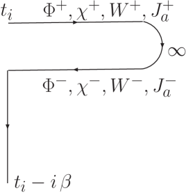
The non-equilibrium action is given by

$$S[\Phi^{\pm},\chi^{\pm};J^{\pm}_{\Phi};J^{\pm}_{\chi};J^{\pm}_{W}] = \int_{t_{i}}^{\infty}dtd^{3}x\,\left[\mathcal{L}_{0}(\phi^{+})+J^{+}_{\phi}\phi^{+}-\mathcal{L}_{0}(\phi^{-})-J^{-}_{\phi}\phi^{-}\right]+$$ (31)

$$\int_{\mathcal{C}}d^{4}x\Big{\{}\mathcal{L}_{0}[\chi,W]+J_{\chi}\chi+J_{W}\,W+G\,\phi_{\alpha}\,\mathcal{O}_{\alpha}+G\phi^{2}_{\alpha}\chi^{2}_{\alpha}\Big{\}}$$

where $\mathcal{C}$ describes the following contour in the complex time plane: along the forward branch $(t_{i},+\infty)$ the fields and sources are $\Phi^{+},\chi^{+},J^{+}_{\chi}$, along the backward branch $(\infty,t_{i})$ the fields and sources are $\Phi^{-},\chi^{-},J^{-}_{\chi}$ and along the Euclidean branch $(t_{i},t_{i}-i\beta)$ the fields and sources are $\Phi=0;\chi^{\beta},J^{\beta}_{\chi}$. Along the Euclidean branch the interaction term vanishes since the initial density matrix for the field $\chi$ is assumed to be that of thermal equilibrium. This contour is depicted in fig. (1)

Figure 1: Contour in time for the non-equilibrium path integral representation.

The trace over the degrees of freedom of the $\chi$ field with the initial equilibrium density matrix, entail periodic boundary conditions for $\chi,W$ along the contour $\mathcal{C}$. However, the boundary conditions on the path integrals for the field $\Phi$ are given by

$$\Phi^{+}(\vec{x},t=\infty)=\Phi^{-}(\vec{x},t=\infty)$$ (32)

and

$$\Phi^{+}(\vec{x},t=t_{i})=\Phi_{i}(\vec{x})\;\;\;;\;\;\;\Phi^{-}(\vec{x},t=t_{i})=\Phi^{\prime}_{i}(\vec{x})$$ (33)

The reason for the different path integrations is that whereas the $\chi$ and $W$ fields are traced over with an initial thermal density matrix, the initial density matrix for the $\Phi$ field will be specified later as part of the initial value problem. The path integral over $\chi,W$ leads to the influence functional for $\Phi^{\pm}$feyver .

Because we are not interested in the correlation functions of the bath fields but only those of the “system” fields, we set the external c-number currents $J_{\chi}=0;J_{W}=0$. Insofar as the bath fields are concerned, the system fields $\Phi$ act as an external c-number source, and tracing over the bath fields leads to

$$\int{\cal D}\chi^{\pm}{\cal D}W^{\pm}{\cal D}\chi^{\beta}{\cal D}W^{\beta}\,e^{i\int_{\mathcal{C}}d^{4}x\Big{\{}\mathcal{L}_{0}[\chi,W]+G\,\phi_{\alpha}\mathcal{O}_{\alpha}+G\phi^{2}_{\alpha}\chi^{2}_{\alpha}\Big{\}}}=\Big{\langle}e^{iG\int_{\mathcal{C}}d^{4}x\phi_{\alpha}\mathcal{O}_{\alpha}+\phi^{2}_{\alpha}\chi^{2}_{\alpha}}\Big{\rangle}_{0}\,\mathrm{Tr}e^{-\beta H^{0}[\chi,W]}.$$ (34)

The expectation value in the right hand side of eqn. (34) is in the equilibrium free field density matrix of the fields $\chi,W$. The path integral can be carried out in perturbation theory and the result exponentiated to yield the effective action as follows

$$\Big{\langle}e^{iG\int_{\mathcal{C}}d^{4}x\phi_{\alpha}\mathcal{O}_{\alpha}+\phi^{2}_{\alpha}\chi^{2}_{\alpha}}\Big{\rangle}_{0}= 1+iG\int_{\mathcal{C}}d^{4}x\Big{\{}\phi_{\alpha}(x)\,\Big{\langle}\mathcal{O}_{\alpha}(x)\Big{\rangle}_{0}+\phi^{2}_{\alpha}(x)\,\Big{\langle}\chi^{2}_{\alpha}(x)\Big{\rangle}_{0}\Big{\}}+$$ (35)

$$\frac{(iG)^{2}}{2}\int_{\mathcal{C}}d^{4}x\int_{\mathcal{C}}d^{4}x^{\prime}\phi_{\alpha}(x)\phi_{\beta}(x^{\prime})\Big{\langle}\mathcal{O}_{\alpha}(x)\mathcal{O}_{\beta}(x^{\prime})\Big{\rangle}_{0}+\mathcal{O}(G^{3})$$

This is the usual expansion of the exponential of the connected correlation functions, therefore this series is identified with

$$\Big{\langle}e^{iG\int_{\mathcal{C}}d^{4}x\phi_{\alpha}\mathcal{O}_{\alpha}+\phi^{2}_{\alpha}\chi^{2}_{\alpha}}\Big{\rangle}_{0}=e^{i\,L_{if}[\phi^{+},\phi^{-}]}\;,$$ (36)

where $L_{if}[\phi^{+},\phi^{-}]$ is the influence functionalfeyver , and $\langle\cdots\rangle_{0}$ stand for expectation values in the bath in equilibrium. For $\Big{\langle}\chi_{\alpha}(x)W(x)\Big{\rangle}_{0}=0$ the influence functional is given by

$$L_{if}[\phi^{+},\phi^{-}]=G\int_{\mathcal{C}}d^{4}x\phi^{2}_{\alpha}(x)\,\Big{\langle}\chi^{2}_{\alpha}(x)\Big{\rangle}_{0}+i\frac{G^{2}}{2}\int_{\mathcal{C}}d^{4}x\int_{\mathcal{C}}d^{4}x^{\prime}\phi_{\alpha}(x)\phi_{\beta}(x^{\prime})\langle\mathcal{O}_{\alpha}(x)\mathcal{O}_{\beta}(x^{\prime})\rangle_{0}+\mathcal{O}(G^{3})\,.$$ (37)

In the above result we have neglected second order contributions of the form $G^{2}\phi^{4}_{\alpha}$. These non-linear contributions give rise to interactions between the quasiparticles and will be neglected in this article. Here we are primarily concerned with establishing the general properties of the quasiparticles and their equilibration with the bath and not with their mutual interaction. As in the case of mixed neutrinos, the inclusion of a “neutrino” background may lead to the phenomenon of non-linear synchronizationpantaleone ; samuel ; synchro2 , but the study of this phenomenon is beyond the realm of this article.

We focus solely on the non-equilibrium effective action up to quadratic order in the “neutrino fields”, from which we extract the dispersion relations, relaxation rates and the approach to equilibrium with the bath of the quasiparticle modes in the medium.

The integrals along the contour $\mathcal{C}$ stand for the following expressions:

$$G\int_{\mathcal{C}}d^{4}x\phi^{2}_{\alpha}(x)\,\Big{\langle}\chi^{2}_{\alpha}(x)\Big{\rangle}_{0}=V_{\alpha\alpha}~{}\int d^{3}x\int_{t_{i}}^{\infty}dt\left[\phi^{2\,+}_{\alpha}(x)-\phi^{2\,-}_{\alpha}(x)\right]$$ (38)

where $V_{\alpha\alpha}$ are the “matter potentials” which are independent of position under the assumption of translational invariance, and time independent under the assumption that the bath is in equilibrium, and

$$\int_{\mathcal{C}}d^{4}x\int_{\mathcal{C}}d^{4}x^{\prime}\phi_{\alpha}(x)\phi_{\beta}(x^{\prime})\langle\mathcal{O}_{\alpha}(x)\mathcal{O}_{\beta}(x^{\prime})\rangle_{0}= \int d^{3}x\int_{t_{i}}^{\infty}dt\int d^{3}x^{\prime}\int_{t_{i}}^{\infty}dt^{\prime}\Big{[}\phi^{+}_{\alpha}(x)\phi^{+}_{\beta}(x^{\prime})\langle\mathcal{O}^{+}_{\alpha}(x)\mathcal{O}^{+}_{\beta}(x^{\prime})\rangle_{0}$$

$$+ \phi^{-}_{\alpha}(x)\phi^{-}_{\beta}(x^{\prime})\langle\mathcal{O}^{-}_{\alpha}(x)\mathcal{O}^{-}_{\beta}(x^{\prime})\rangle_{0}-\phi^{+}_{\alpha}(x)\phi^{-}_{\beta}(x^{\prime})\langle\mathcal{O}^{+}_{\alpha}(x)\mathcal{O}^{-}_{\beta}(x^{\prime})\rangle_{0}$$

$$- \phi^{-}_{\alpha}(x)\phi^{+}_{\beta}(x^{\prime})\langle\mathcal{O}^{-}_{\alpha}(x)\mathcal{O}^{+}_{\beta}(x^{\prime})\rangle_{0}\Big{]}$$ (39)

Since the expectation values above are computed in a thermal equilibrium translational invariant density matrix, it is convenient to introduce the spatial Fourier transform of the composite operator ${\cal O}$ in a spatial volume $V$ as

$${\cal O}_{\alpha,\vec{k}}(t)=\frac{1}{\sqrt{V}}\int d^{3}xe^{i\vec{k}\cdot\vec{x}}{\cal O}_{\alpha}(\vec{x},t)$$ (40)

in terms of which we obtain following the correlation functions

$$\langle\mathcal{O}^{-}_{\alpha,\vec{k}}(t){\cal O}^{+}_{\beta,-\vec{k}}(t^{\prime})\rangle=\mathrm{Tr}\,{\cal O}_{\beta,-\vec{k}}(t^{\prime})\,e^{-\beta\,H^{0}[\chi,W]}\,\mathcal{O}_{\alpha,\vec{k}}(t)=\mathcal{G}^{>}_{\alpha\beta}(k;t-t^{\prime})\equiv{\cal G}^{-+}_{\alpha\beta}(k;t-t^{\prime})$$ (41)

$$\langle{\cal O}^{+}_{\alpha,\vec{k}}(t){\cal O}^{-}_{\beta,-\vec{k}}(t^{\prime})\rangle=\mathrm{Tr}\,\mathcal{O}_{\alpha,\vec{k}}(t)\,e^{-\beta\,H_{\chi}}\,{\cal O}_{\beta,-\vec{k}}(t^{\prime})={\cal G}^{<}_{\alpha\beta}(k;t-t^{\prime})\equiv{\cal G}^{+-}_{\alpha\beta}(k;t-t^{\prime})={\cal G}^{-+}_{\beta,\alpha}(k;t^{\prime}-t)$$ (42)

$$\langle{\cal O}^{+}_{\alpha,\vec{k}}(t){\cal O}^{+}_{\beta,-\vec{k}}(t^{\prime})\rangle={\cal G}^{>}_{\alpha\beta}(k;t-t^{\prime})\Theta(t-t^{\prime})+{\cal G}^{<}_{\alpha\beta}(k;t-t^{\prime})\Theta(t^{\prime}-t)\equiv{\cal G}^{++}_{\alpha\beta}(k;t-t^{\prime})$$ (43)

$$\langle{\cal O}^{-}_{\alpha,\vec{k}}(t){\cal O}^{-}_{\beta,-\vec{k}}(t^{\prime})\rangle={\cal G}^{>}_{\alpha\beta}(k;t-t^{\prime})\Theta(t^{\prime}-t)+{\cal G}^{<}_{\alpha\beta}(k;t-t^{\prime})\Theta(t-t^{\prime})={\cal G}^{--}_{\alpha\beta}(k;t-t^{\prime})$$ (44)

The time evolution of the operators is determined by the Heisenberg picture of $H_{0}[\chi,W]$. Because the density matrix for the bath is in equilibrium, the correlation functions above are solely functions of the time difference as made explicit in the expressions above. These correlation functions are not independent, but obey

$$\mathcal{G}^{++}_{\alpha\beta}(k;t,t^{\prime})+\mathcal{G}^{--}_{\alpha\beta}(k;t,t^{\prime})-\mathcal{G}^{-+}_{\alpha\beta}(k;t,t^{\prime})-\mathcal{G}^{+-}_{\alpha\beta}(k;t,t^{\prime})=0$$ (45)

The correlation function $\mathcal{G}^{>}_{\alpha\beta}$ up to lowest order in the coupling $G$ is given by

$$\mathcal{G}^{>}_{\alpha\beta}(k;t-t^{\prime})=\int\frac{d^{3}p}{(2\pi)^{3}}\langle W_{\vec{p}+\vec{k}}(t)W_{-\vec{p}-\vec{k}}(t^{\prime})\rangle\langle\chi_{\vec{p},\alpha}(t)\chi_{-\vec{p},\beta}(t^{\prime})\rangle$$ (46)

where the expectation value is in the free field equilibrium density matrix of the respective fields. This correlation function is diagonal in the flavor basis and this entails that all the Green’s functions (41-44) are diagonal in the flavor basis.

The non-equilibrium effective action yields the time evolution of the reduced density matrix, it is given by

$$L_{eff}[\phi^{+},\phi^{-}]=\int_{t_{i}}^{\infty}dtd^{3}x\,\left[\mathcal{L}_{0}(\phi^{+})-\mathcal{L}_{0}(\phi^{-})\right]+L_{if}[\phi^{+},\phi^{-}]$$ (47)

where we have set the sources $J^{\pm}$ for the fields $\phi^{\pm}$ to zero.

In what follows we take $t_{i}=0$ without loss of generality since (i) for $t>t_{i}$ the total Hamiltonian is time independent and the correlations will be solely functions of $t-t_{i}$, and (ii) we will be ultimately interested in the limit $t\gg t_{i}$ when all transient phenomena has relaxed. Adapting the methods presented in ref. hoboydavey to account for the matrix structure of the effective action, introducing the spatial Fourier transform of the fields $\phi^{\pm}$ defined as in eqn. (40) and the matrix of the matter potentials

$$\mathds{V}=\left(\begin{array}[]{cc}V_{ee}&0\\ 0&V_{\mu\mu}\\ \end{array}\right)$$ (48)

we find

$$iL_{eff}[\phi^{+},\phi^{-}] = \sum_{\vec{k}}\Bigg{\{}\frac{i}{2}\int_{0}^{\infty}dt\Big{[}\dot{\phi}^{+}_{\alpha,\vec{k}}(t)\dot{\phi}^{+}_{\alpha,-\vec{k}}(t)-\phi^{+}_{\alpha,\vec{k}}(t)(k^{2}\,\delta_{\alpha\beta}+\mathbb{M}^{2}_{\alpha\beta}+\mathds{V}_{\alpha\beta})\phi^{+}_{\beta,-\vec{k}}(t)$$ (49)

$$-\dot{\phi}^{-}_{\alpha,\vec{k}}(t)\dot{\phi}^{-}_{\alpha,-\vec{k}}(t)+\phi^{-}_{\alpha,\vec{k}}(t)(k^{2}\,\delta_{\alpha\beta}+\mathbb{M}^{2}_{\alpha\beta}+\mathds{V}_{\alpha\beta})\phi^{-}_{\beta,-\vec{k}}(t)\Big{]}$$

$$-\frac{G^{2}}{2}\int_{0}^{\infty}dt\int_{0}^{\infty}dt^{\prime}\left[\phi^{+}_{\alpha,\vec{k}}(t){\cal G}^{++}_{\alpha\beta}(k;t,t^{\prime})\phi^{+}_{\beta,-\vec{k}}(t^{\prime})+\phi^{-}_{\alpha,\vec{k}}(t){\cal G}^{--}_{\alpha\beta}(k;t,t^{\prime})\phi^{-}_{\beta,-\vec{k}}(t^{\prime})\right.$$

$$\left.-\phi^{+}_{\alpha,\vec{k}}(t){\cal G}^{+-}_{\alpha\beta}(k;t,t^{\prime})\phi^{-}_{\beta,-\vec{k}}(t^{\prime})-\phi^{-}_{\alpha,\vec{k}}(t){\cal G}^{-+}_{\alpha\beta}(k;t,t^{\prime})\phi^{+}_{\beta,-\vec{k}}(t^{\prime})\right]\Bigg{\}}$$

The “matter potentials” $V_{\alpha\alpha}$ play the role of the index of refraction correction to the dispersion relationsnotzold and is of first order in the coupling $G$ whereas the contributions that involve $\mathcal{G}$ are of order $G^{2}$. As it will become clear below, it is more convenient to introduce the Wigner center of mass and relative variables

$$\Psi_{\alpha}(\vec{x},t)=\frac{1}{2}\left(\phi^{+}_{\alpha}(\vec{x},t)+\phi^{-}_{\alpha}(\vec{x},t)\right)\;\;;\;\;R_{\alpha}(\vec{x},t)=\left(\phi^{+}_{\alpha}(\vec{x},t)-\phi^{-}_{\alpha}(\vec{x},t)\right)$$ (50)

and the Wigner transform of the initial density matrix for the $\phi$ fields

$${\cal W}(\Psi^{0};\Pi^{0})=\int DR_{0,\alpha}e^{-i\int d^{3}x\Pi_{0,\alpha}(\vec{x})R_{0,\alpha}(\vec{x})}\rho(\Psi^{0}+\frac{R^{0}}{2};\Psi^{0}-\frac{R^{0}}{2})$$ (51)

with the inverse transform

$$\rho(\Psi^{0}+\frac{R^{0}}{2};\Psi^{0}-\frac{R^{0}}{2})=\int D\Pi^{0}_{\alpha}e^{i\int d^{3}x\Pi^{0}_{\alpha}(\vec{x})R^{0}_{\alpha}(\vec{x})}{\cal W}(\Psi^{0};\Pi^{0})$$ (52)

The boundary conditions on the $\phi$ path integral given by (33) translate into the following boundary conditions on the center of mass and relative variables

$$\Psi_{\alpha}(\vec{x},t=0)=\Psi^{0}_{\alpha}\;\;;\;\;R_{\alpha}(\vec{x},t=0)=R^{0}_{\alpha}$$ (53)

furthermore, the boundary condition (32) yields the following boundary condition for the relative field

$$R_{\alpha}(\vec{x},t=\infty)=0.$$ (54)

This observation will be important in the steps that follow.

The same description applies to the fields in the mass basis. We will treat both cases on equal footing with the notational difference that Greek labels $\alpha,\beta$ refer to the flavor and Latin indices $i,j$ refer to the mass basis.

In terms of the spatial Fourier transforms of the center of mass and relative variables (50) introduced above, integrating by parts and accounting for the boundary conditions (53), the non-equilibrium effective action (49) becomes:

$$iL_{eff}[\Psi,R] = \int_{0}^{\infty}dt\sum_{\vec{k}}\left\{-iR_{\alpha,-\vec{k}}\left(\ddot{\Psi}_{\alpha,\vec{k}}(t)+(k^{2}\delta_{\alpha\beta}+\mathbb{M}^{2}_{\alpha\beta}+\mathds{V}_{\alpha\beta})\Psi_{\beta,\vec{k}}(t)\right)\right\}$$ (55)

$$- \int_{0}^{\infty}dt\int_{0}^{\infty}dt^{\prime}\sum_{\vec{k}}\left\{\frac{1}{2}R_{\alpha,-\vec{k}}(t){\cal K}_{\alpha\beta}(k;t-t^{\prime})R_{\beta,\vec{k}}(t^{\prime})+R_{\alpha,-\vec{k}}(t)\,i\Sigma^{R}_{\alpha\beta}(k;t-t^{\prime})\Psi_{\beta,\vec{k}}(t^{\prime})\right\}$$

$$+ i\int d^{3}xR^{0}_{\alpha}(\vec{x})\dot{\Psi}_{\alpha}(\vec{x},t=0)$$

where the last term arises after the integration by parts in time, using the boundary conditions (53) and (54). The kernels in the above effective Lagrangian are given by (see eqns. (41-44))

$$\mathcal{K}_{\alpha\beta}(k;t-t^{\prime}) = \frac{G^{2}}{2}\left[{\cal G}^{>}_{\alpha\beta}(k;t-t^{\prime})+{\cal G}^{<}_{\alpha\beta}(k;t-t^{\prime})\right]$$ (56)

$$i\Sigma^{R}_{\alpha\beta}(k;t-t^{\prime}) = G^{2}\left[{\cal G}^{>}_{\alpha\beta}(k;t-t^{\prime})-{\cal G}^{<}_{\alpha\beta}(k;t-t^{\prime})\right]\Theta(t-t^{\prime})\equiv i\Sigma_{\alpha\beta}(k;t-t^{\prime})\Theta(t-t^{\prime})$$ (57)

The term quadratic in the relative variable $R$ can be written in terms of a stochastic noise as

$$\exp\Big{\{}-\frac{1}{2}\int dt\int dt^{\prime}R_{\alpha,-\vec{k}}(t){\cal K}_{\alpha\beta}(k;t-t^{\prime})R_{\beta\vec{k}}(t^{\prime})\Big{\}}=\int{\cal D}\xi \exp\Big{\{}-\frac{1}{2}\int dt\int dt^{\prime}\,\xi_{\alpha,\vec{k}}(t){\cal K}^{-1}_{\alpha\beta}(k;t-t^{\prime})\xi_{\beta,-\vec{k}}(t^{\prime})$$ (58)

$$+i\int dt\,\xi_{\alpha,-\vec{k}}(t)R_{\alpha,\vec{k}}(t)\Big{\}}$$

The non-equilibrium generating functional can now be written in the following form

$${\cal Z} = \int D\Psi^{0}\int D\Pi^{0}\int{\cal D}\Psi{\cal D}R{\cal D}\xi~{}~{}{\cal W}(\Psi^{0};\Pi^{0})DR^{0}e^{i\int d^{3}xR_{0,\alpha}(\vec{x})\left(\Pi^{0}_{\alpha}(\vec{x})-\dot{\Psi}_{\alpha}(\vec{x},t=0)\right)}{\cal P}[\xi]$$

$$\exp\left\{-i\int_{0}^{\infty}dt\,R_{\alpha,-\vec{k}}(t)\left[\ddot{\Psi}_{\alpha,\vec{k}}(t)+(k^{2}\,\delta_{\alpha\beta}+\mathbb{M}^{2}_{\alpha\beta}+\mathds{V}_{\alpha\beta})\Psi_{\beta,\vec{k}}(t)+\int dt^{\prime}\,\Sigma^{R}_{\alpha\beta}(k;t-t^{\prime})\Psi_{\beta,\vec{k}}(t^{\prime})-\xi_{\alpha,\vec{k}}(t)\right]\right\}$$

$${\cal P}[\xi] = \exp\left\{-\frac{1}{2}\int_{0}^{\infty}dt\int_{0}^{\infty}dt^{\prime}~{}~{}\xi_{\alpha,\vec{k}}(t){\cal K}^{-1}_{\alpha\beta}(k;t-t^{\prime})\xi_{\beta,-\vec{k}}(t^{\prime})\right\}$$ (60)

The functional integral over $R^{0}$ can now be done, resulting in a functional delta function, that fixes the boundary condition $\dot{\Psi}_{\alpha}(\vec{x},t=0)=\Pi^{0}_{\alpha}(\vec{x})$. Finally the path integral over the relative variable can be performed, leading to a functional delta function and the final form of the generating functional given by

$${\cal Z} = \int D\Psi^{0}D\Pi^{0}\,{\cal W}(\Psi^{0};\Pi^{0}){\cal D}\Psi{\cal D}\xi\,{\cal P}[\xi]\,\times$$ (61)

$$\delta\left[\ddot{\Psi}_{\alpha,\vec{k}}(t)+(k^{2}\,\delta_{\alpha\beta}+\mathbb{M}^{2}_{\alpha\beta}+\mathds{V}_{\alpha\beta})\Psi_{\beta,\vec{k}}(t)+\int_{0}^{t}dt^{\prime}~{}\Sigma_{\alpha\beta}(k;t-t^{\prime})\Psi_{\beta,\vec{k}}(t^{\prime})-\xi_{\alpha,\vec{k}}(t)\right]$$

with the boundary conditions on the path integral on $\Psi$ given by

$$\Psi_{\alpha}(\vec{x},t=0)=\Psi^{0}_{\alpha}(\vec{x})\;\;;\;\;\dot{\Psi}_{\alpha}(\vec{x},t=0)=\Pi^{0}_{\alpha}(\vec{x})\,,$$ (62)

where we have used the definition of $\Sigma^{R}_{\alpha\beta}(k;t-t^{\prime})$ in terms of $\Sigma_{\alpha\beta}(k;t-t^{\prime})$ given in equation (57).

The meaning of the above generating functional is the following: to obtain correlation functions of the center of mass Wigner variable $\Psi$ we must first find the solution of the classical stochastic Langevin equation of motion

$$\ddot{\Psi}_{\alpha,\vec{k}}(t)+(k^{2}\,\delta_{\alpha\beta}+\mathbb{M}^{2}_{\alpha\beta}+\mathds{V}_{\alpha\beta})\Psi_{\beta,\vec{k}}(t)+\int_{0}^{t}dt^{\prime}~{}\Sigma_{\alpha\beta}(k;t-t^{\prime})\Psi_{\beta,\vec{k}}(t^{\prime})=\xi_{\alpha,\vec{k}}(t)$$

$$\Psi_{\alpha,\vec{k}}(t=0)=\Psi^{0}_{\alpha,\vec{k}}~{}~{};~{}~{}\dot{\Psi}_{\alpha,\vec{k}}(t=0)=\Pi^{0}_{\alpha,\vec{k}}$$ (63)

for arbitrary noise term $\xi$ and then average the products of $\Psi$ over the stochastic noise with the Gaussian probability distribution ${\cal P}[\xi]$ given by (60), and finally average over the initial configurations $\Psi^{0}(\vec{x});\Pi^{0}(\vec{x})$ weighted by the Wigner function ${\cal W}(\Psi^{0},\Pi^{0})$, which plays the role of an initial phase space distribution function.

Calling the solution of (63) $\Psi_{\alpha,\vec{k}}(t;\xi;\Psi_{i};\Pi_{i})$, the two point correlation function, for example, is given by

$$\langle\Psi_{\alpha,\vec{k}}(t)\Psi_{\beta,-\vec{k}}(t^{\prime})\rangle=\frac{\int{\cal D}[\xi]{\cal P}[\xi]\int D\Psi^{0}\int D\Pi^{0}~{}~{}{\cal W}(\Psi^{0};\Pi^{0})\Psi_{\alpha,\vec{k}}(t;\xi;\Psi^{0};\Pi^{0})\Psi_{\beta,-\vec{k}}(t^{\prime};\xi;\Psi^{0};\Pi^{0})}{\int{\cal D}[\xi]{\cal P}[\xi]\int D\Psi^{0}\int D\Pi^{0}~{}~{}{\cal W}(\Psi^{0};\Pi^{0})}\,.$$ (64)

In computing the averages and using the functional delta function to constrain the configurations of $\Psi$ to the solutions of the Langevin equation, there is the Jacobian of the operator $(d^{2}/dt^{2}+k^{2})\delta_{\alpha\beta}+\mathbb{M}^{2}+\mathds{V}+\int dt^{\prime}\Sigma^{ret}(k;t-t^{\prime})$ which however, is independent of the field and the noise and cancels between numerator and denominator in the averages. There are two different averages:

• The average over the stochastic noise term, which up to this order is Gaussian. We denote the average of a functional $\mathcal{F}[\xi]$ over the noise with the probability distribution function $P[\xi]$ given by eqn. (60) as

  $$\langle\langle\mathcal{F}\rangle\rangle\equiv\frac{\int\mathcal{D}\xi P[\xi]\mathcal{F}[\xi]}{\int\mathcal{D}\xi P[\xi]}.$$ (65)

  Since the noise probability distribution function is Gaussian the only necessary correlation functions for the noise are given by

  $$\langle\langle\xi_{\alpha,\vec{k}}(t)\rangle\rangle=0\;,\;\langle\langle\xi_{\alpha,\vec{k}}(t)\xi_{\beta,\vec{k}^{\prime}}(t^{\prime})\rangle\rangle={\mathcal{K}}_{\alpha\beta}(k;t-t^{\prime})\,\delta^{3}(\vec{k}+\vec{k}^{\prime})$$ (66)

  and the higher order correlation functions are obtained from Wick’s theorem as befits a Gaussian distribution function. Because the noise kernel $\mathcal{K}_{\alpha\beta}(k;t-t^{\prime})\neq\delta(t-t^{\prime})$ the noise is colored.

• The average over the initial conditions with the Wigner distribution function ${\cal W}(\Psi^{0},\Pi^{0})$ which we denote as

  $$\overline{\mathcal{A}[\Psi^{0},\Pi^{0}]}\equiv\frac{\int D\Psi^{0}\int D\Pi^{0}~{}~{}{\cal W}(\Psi^{0};\Pi^{0})\mathcal{A}[\Psi^{0},\Pi^{0}]}{\int D\Psi^{0}\int D\Pi^{0}~{}~{}{\cal W}(\Psi^{0};\Pi^{0})}$$ (67)

Therefore, the average in the time evolved reduced density matrix implies two distinct averages: an average over the initial conditions of the system fields and and average over the noise distribution function. The total average is defined by

$$\langle\cdots\rangle\equiv\overline{\langle\langle\cdots\rangle\rangle}~{}~{}.$$ (68)

Equal time expectation values and correlation functions are simply expressed in terms of the center of mass Wigner variable $\Psi$ as can be seen as follows: the expectation values of the field

$$\langle\phi^{+}(\vec{x},t)\rangle=\mathrm{Tr}\phi(\vec{x},t)\rho(t)~{}~{};~{}~{}\langle\phi^{-}(\vec{x},t)\rangle=\mathrm{Tr}\rho(t)\phi(\vec{x},t)$$ (69)

hence the total average (68) is given by

$$\langle\phi(\vec{x},t)\rangle=\langle\Psi(\vec{x},t)\rangle\,.$$ (70)

Similarly the equal time correlation functions obey

$$\langle\phi^{+}(\vec{x},t)\phi^{+}(\vec{x}^{\prime},t)\rangle=\langle\phi^{+}(\vec{x},t)\phi^{-}(\vec{x}^{\prime},t)\rangle=\langle\phi^{-}(\vec{x},t)\phi^{+}(\vec{x}^{\prime},t)\rangle=\langle\phi^{-}(\vec{x},t)\phi^{-}(\vec{x}^{\prime},t)\rangle=\langle\Psi(\vec{x},t)\Psi(\vec{x}^{\prime},t)\rangle\,.$$ (71)

Therefore the center of mass variables $\Psi$ contain all the information necessary to obtain expectation values and equal time correlation functions.

III.1 One body density matrix and equilibration:

We study equilibration by focusing on the one-body density matrix

$$\rho_{\alpha\beta}(k;t)=\mathrm{Tr}\rho(0)\phi_{\alpha}(\vec{k},t)\phi_{\beta}(-\vec{k},t)=\mathrm{Tr}\rho(t)\phi_{\alpha}(\vec{k},0)\phi_{\beta}(-\vec{k},0)$$ (72)

where

$$\rho(t)=e^{-iHt}\rho(0)e^{iHt}$$ (73)

is the time evolved density matrix. The time evolution of the one-body density matrix obeys the Liouville-type equation

$$\frac{d}{dt}\rho_{\alpha\beta}(t)=-i\mathrm{Tr}\big{[}H,\rho(t)\big{]}\phi_{\alpha}(\vec{k},0)\phi_{\beta}(-\vec{k},0)\,.$$ (74)

If the system reaches equilibrium with the bath at long times, then it is expected that

$$\big{[}H,\rho(t)\big{]}\,\stackrel{{\scriptstyle t\rightarrow\infty}}{{\longrightarrow~{}~{}0}}$$ (75)

Therefore the asymptotically long time limit of the one-body density matrix yields information on whether the density matrix is diagonal in the flavor or any other basis. Hence we seek to obtain

$$\rho_{\alpha\beta}(k;\infty)=\mathrm{Tr}\rho(\infty)\phi_{\alpha}(\vec{k},0)\phi_{\beta}(-\vec{k},0)=\langle\Psi_{\alpha\vec{k}}(\infty)\Psi_{\beta,-\vec{k}}(\infty)\rangle\,.$$ (76)

and to establish the basis in which it is nearly diagonal. The second equality in eqn. (76) follows from eq. (71), and the average is defined by eq.(68). To establish a guide post, consider the one-body density matrix for the free “neutrino fields” in thermal equilibrium, for which the equilibrium density matrix is

$$\rho_{eq}=e^{-\beta H_{0}[\varphi]}$$ (77)

where $H_{0}[\varphi]$ is the free “neutrino” Hamiltonian. This density matrix is diagonal in the basis of mass eigenstates and so is the one-body density matrix which in the mass basis is given by

$$\rho_{ij}(k)=\left(\begin{array}[]{cc}\frac{1}{2\omega_{1}(k)}\coth\left[\frac{\beta\omega_{1}(k)}{2}\right]&0\\ 0&\frac{1}{2\omega_{2}(k)}\coth\left[\frac{\beta\omega_{2}(k)}{2}\right]\\ \end{array}\right)~{}~{};~{}~{}i,j=1,2$$ (78)

therefore in the flavor basis the one-body density matrix is given by

$$\rho_{\alpha\beta}(k)=U(\theta)~{}\left(\begin{array}[]{cc}\frac{1}{2\omega_{1}(k)}\coth\left[\frac{\beta\omega_{1}(k)}{2}\right]&0\\ 0&\frac{1}{2\omega_{2}(k)}\coth\left[\frac{\beta\omega_{2}(k)}{2}\right]\\ \end{array}\right)~{}U^{-1}(\theta)~{}~{};~{}~{}\alpha,\beta=e,\mu$$ (79)

This simple example provides a guide to interpret the approach to equilibrium. Including interactions there is a competition between the mass and flavor basis. The interaction is diagonal in the flavor basis, while the unperturbed Hamiltonian is diagonal in the mass basis, this of course is the main physical reason behind neutrino oscillations. In the presence of interactions, the correct form of the equilibrium one-body density matrix can only be obtained from the asymptotic long time limit of the time-evolved density matrix.

III.2 Generalized fluctuation-dissipation relation:

From the expressions (56) and (57) in terms of the Wightmann functions (41,42) which are averages in the equilibrium density matrix of the bath fields ($\chi,W$), we obtain a dispersive representation for the kernels $\mathcal{K}_{\alpha\beta}(k;t-t^{\prime});\Sigma^{R}_{\alpha\beta}(k;t-t^{\prime})$. This is achieved by writing the expectation value in terms of energy eigenstates of the bath, introducing the identity in this basis, and using the time evolution of the Heisenberg field operators to obtain

$$G^{2}~{}{\cal G}^{>}_{\alpha\beta}(k;t-t^{\prime})=\int^{\infty}_{-\infty}d\omega~{}\sigma^{>}_{\alpha\beta}(\vec{k},\omega)~{}e^{i\omega(t-t^{\prime})}~{}~{};~{}~{}G^{2}~{}{\cal G}^{<}_{\alpha\beta}(k;t-t^{\prime})=\int^{\infty}_{-\infty}d\omega~{}\sigma^{<}_{\alpha\beta}(\vec{k},\omega)~{}e^{i\omega(t-t^{\prime})}$$ (80)

with the spectral functions

$$\sigma^{>}_{\alpha\beta}(\vec{k},\omega) = \frac{G^{2}}{\mathcal{Z}_{b}}\sum_{m,n}e^{-\beta E_{n}}\langle n|{\cal O}_{\alpha,\vec{k}}(0)|m\rangle\langle m|{\cal O}_{\beta,-\vec{k}}(0)|n\rangle\,\delta(\omega-(E_{n}-E_{m}))$$ (81)

$$\sigma^{<}_{\alpha\beta}(\vec{k},\omega) = \frac{G^{2}}{\mathcal{Z}_{b}}\sum_{m,n}e^{-\beta E_{m}}\langle n|{\cal O}_{\beta,-\vec{k}}(0)|m\rangle\langle m|{\cal O}_{\alpha,\vec{k}}(0)|n\rangle\,\delta(\omega-(E_{m}-E_{n}))$$ (82)

where $\mathcal{Z}_{b}=\mathrm{Tr}\,e^{-\beta H_{\chi}}$ is the equilibrium partition function of the “bath” and in the above expressions the averages are solely with respect to the bath variables. Upon relabelling $m\leftrightarrow n$ in the sum in the definition (82) and using the fact that these correlation functions are parity and rotational invariantkapusta and diagonal in the flavor basis we find the Kubo-Martin-Schwinger (KMS) relationkapusta

$$\sigma^{<}_{\alpha\beta}(k,\omega)=\sigma^{>}_{\alpha\beta}(k,-\omega)=e^{\beta\omega}\sigma^{>}_{\alpha\beta}(k,\omega)\,.$$ (83)

Using the spectral representation of the $\Theta(t-t^{\prime})$ we find the following representation for the retarded self-energy

$$\Sigma^{R}_{\alpha\beta}(k;t-t^{\prime})=\int_{-\infty}^{\infty}\frac{dk_{0}}{2\pi}e^{ik_{0}(t-t^{\prime})}\widetilde{\Sigma}^{R}_{\alpha\beta}(k;k_{0})$$ (84)

with

$$\widetilde{\Sigma}^{R}_{\alpha\beta}(k;k_{0})=\int_{-\infty}^{\infty}d\omega\frac{[\sigma^{>}_{\alpha\beta}(k;\omega)-\sigma^{<}_{\alpha\beta}(k;\omega)]}{\omega-k_{0}+i\epsilon}\,.$$ (85)

Using the condition (83) the above spectral representation can be written in a more useful manner as

$$\widetilde{\Sigma}^{R}_{\alpha\beta}(k;k_{0}) = -\frac{1}{\pi}\int_{-\infty}^{\infty}d\omega\frac{\mathrm{Im}\widetilde{\Sigma}^{R}_{\alpha\beta}(k;\omega)}{\omega-k_{0}+i\epsilon}\,,$$ (86)

where the imaginary part of the self-energy is given by

$$\mathrm{Im}\widetilde{\Sigma}^{R}_{\alpha\beta}(k;\omega) = \pi\sigma^{>}_{\alpha\beta}(k;\omega)\left[e^{\beta\omega}-1\right]$$ (87)

and is positive for $\omega>0$. Equation (83) entails that the imaginary part of the retarded self-energy is an odd function of frequency, namely

$$\mathrm{Im}\widetilde{\Sigma}^{R}_{\alpha\beta}(k;\omega)=-\mathrm{Im}\widetilde{\Sigma}^{R}_{\alpha\beta}(k;-\omega)\;.$$ (88)

The relation (87) leads to the following results which will be useful later

$$\sigma^{>}_{\alpha\beta}(k;\omega)=\frac{1}{\pi}\mathrm{Im}\widetilde{\Sigma}^{R}_{\alpha\beta}(k;\omega)\,n(\omega)~{}~{};~{}~{}\sigma^{<}_{\alpha\beta}(k;\omega)=\frac{1}{\pi}\mathrm{Im}\widetilde{\Sigma}^{R}_{\alpha\beta}(k;\omega)\,\left[1+n(\omega)\right]$$ (89)

where $n(\omega)=[e^{\beta\omega}-1]^{-1}$ is the Bose-Einstein distribution function. Similarly from the definitions (56) and (80) and the condition (83) we find

$$\mathcal{K}_{\alpha\beta}(k;t-t^{\prime}) = \int_{-\infty}^{\infty}\frac{dk_{0}}{2\pi}e^{ik_{0}(t-t^{\prime})}\widetilde{\mathcal{K}}_{\alpha\beta}(k;k_{0})$$ (90)

$$\widetilde{\mathcal{K}}_{\alpha\beta}(k;k_{0}) = \pi\sigma^{>}_{\alpha\beta}(k;k_{0})\left[e^{\beta k_{0}}+1\right]$$ (91)

whereupon using the condition (83) leads to the generalized fluctuation-dissipation relation

$$\widetilde{\mathcal{K}}_{\alpha\beta}(k;k_{0})=\mathrm{Im}\widetilde{\Sigma}^{R}_{\alpha\beta}(k;k_{0})\coth\left[\frac{\beta k_{0}}{2}\right]\,.$$ (92)

Thus we see that $\mathrm{Im}\widetilde{\Sigma}^{R}_{\alpha\beta}(k;k_{0})\,;\,\widetilde{\mathcal{K}}_{\alpha\beta}(k;k_{0})$ are odd and even functions of frequency respectively.

For the analysis below we also need the following representation (see eqn. (57))

$$\Sigma_{\alpha\beta}(k;t-t^{\prime})=-i\int_{-\infty}^{\infty}e^{i\omega(t-t^{\prime})}\left[\sigma^{>}_{\alpha\beta}(k;\omega)-\sigma^{<}_{\alpha\beta}(k;\omega)\right]d\omega=\frac{i}{\pi}\int_{-\infty}^{\infty}e^{i\omega(t-t^{\prime})}\mathrm{Im}\widetilde{\Sigma}^{R}_{\alpha\beta}(k;\omega)d\omega$$ (93)

whose Laplace transform is given by

$$\widetilde{\Sigma}_{\alpha\beta}(k;s)\equiv\int^{\infty}_{0}dte^{-st}\Sigma_{\alpha\beta}(k;t)=-\frac{1}{\pi}\int^{\infty}_{-\infty}\frac{\mathrm{Im}\widetilde{\Sigma}^{R}_{\alpha\beta}(k;\omega)}{\omega+is}d\omega$$ (94)

This spectral representation, combined with (86) lead to the relation

$$\widetilde{\Sigma}^{R}_{\alpha\beta}(k;k_{0})=\widetilde{\Sigma}_{\alpha\beta}(k;s=ik_{0}+\epsilon)$$ (95)

The self energy and noise correlation kernels $\widetilde{\Sigma},\widetilde{\mathcal{K}}$ are diagonal in the flavor basis because the interaction is diagonal in this basis. Namely, in the flavor basis

$$\widetilde{\Sigma}(k,\omega)=\Bigg{(}\begin{array}[]{cc}\widetilde{\Sigma}_{ee}(k,\omega)&0\\ 0&\widetilde{\Sigma}_{\mu\mu}(k,\omega)\end{array}\Bigg{)}~{}~{};~{}~{}\widetilde{\mathcal{K}}=[1+2n(\omega)]\,\mathrm{Im}\widetilde{\Sigma}(k,\omega)=\Bigg{(}\begin{array}[]{cc}\widetilde{\mathcal{K}}_{ee}(k,\omega)&0\\ 0&\widetilde{\mathcal{K}}_{\mu\mu}(k,\omega)\end{array}\Bigg{)}\,.$$ (96)

In the mass basis these kernels are given by

$$\widetilde{\Sigma}=\frac{1}{2}\Big{(}\widetilde{\Sigma}_{ee}+\widetilde{\Sigma}_{\mu\mu}\Big{)}\,\mathds{1}+\frac{1}{2}\Big{(}\widetilde{\Sigma}_{ee}-\widetilde{\Sigma}_{\mu\mu}\Big{)}\,\Bigg{(}\begin{array}[]{cc}\cos 2\theta&\sin 2\theta\\ \sin 2\theta&-\cos 2\theta\end{array}\Bigg{)}$$ (97)

and

$$\widetilde{\mathcal{K}}=\frac{1}{2}\Big{(}\widetilde{\mathcal{K}}_{ee}+\widetilde{\mathcal{K}}_{\mu\mu}\Big{)}\,\mathds{1}+\frac{1}{2}\Big{(}\widetilde{\mathcal{K}}_{ee}-\widetilde{\mathcal{K}}_{\mu\mu}\Big{)}\,\Bigg{(}\begin{array}[]{cc}\cos 2\theta&\sin 2\theta\\ \sin 2\theta&-\cos 2\theta\end{array}\Bigg{)}\,.$$ (98)

IV Dynamics: solving the Langevin equation

The solution of the equation of motion (63) can be found by Laplace transform. Define the Laplace transforms

$$\widetilde{\Psi}_{\alpha,\vec{k}}(s)=\int^{\infty}_{0}dte^{-st}\Psi_{\alpha;\vec{k}}(t)~{}~{};~{}~{}\widetilde{\xi}_{\alpha,\vec{k}}(s)=\int^{\infty}_{0}dte^{-st}\xi_{\alpha,\vec{k}}(t)$$ (99)

along with the Laplace transform of the self-energy given by eqn. (94). The Langevin equation in Laplace variable becomes the following algebraic matrix equation

$$\Bigg{[}(s^{2}+k^{2})\delta_{\alpha\beta}+\mathbb{M}^{2}_{\alpha\beta}+\mathds{V}_{\alpha\beta}+\widetilde{\Sigma}_{\alpha\beta}(k;s)\Bigg{]}\widetilde{\Psi}_{\beta,\vec{k}}(s)=\Pi_{0,\alpha,\vec{k}}+s\,\Psi_{0,\alpha,\vec{k}}+\widetilde{\xi}_{\alpha,\vec{k}}(s)$$ (100)

where we have used the initial conditions (62). The solution in real time can be written in a more compact manner as follows. Introduce the matrix function

$$\widetilde{G}(k;s)=\Bigg{[}(s^{2}+k^{2})\mathds{1}+\mathbb{M}^{2}+\mathds{V}+\widetilde{\Sigma}(k;s)\Bigg{]}^{-1}$$ (101)

and its anti-Laplace transform

$$G_{\alpha\beta}(k;t)=\int_{\mathcal{C}}\frac{ds}{2\pi i}\,\widetilde{G}_{\alpha\beta}(k;s)\,e^{st}$$ (102)

where $\mathcal{C}$ refers to the Bromwich contour, parallel to the imaginary axis in the complex $s$ plane to the right of all the singularities of $\widetilde{G}(k;s)$. This function obeys the initial conditions

$$G_{\alpha\beta}(k;0)=0~{}~{};~{}~{}\dot{G}_{\alpha\beta}(k;0)=1\,.$$ (103)

In terms of this auxiliary function the solution of the Langevin equation (63) in real time is given by

$$\Psi_{\alpha,\vec{k}}(t;\Psi^{0};\Pi^{0};\xi)=\dot{G}_{\alpha\beta}(k;t)\,\Psi^{0}_{\beta\vec{k}}+{G}_{\alpha\beta}(k;t)\,\Pi^{0}_{\beta,\vec{k}}+\int^{t}_{0}G_{\alpha\beta}(k;t^{\prime})~{}\xi_{\beta,\vec{k}}(t-t^{\prime})dt^{\prime}\,,$$ (104)

where the dot stands for derivative with respect to time. In the flavor basis we find

$$\widetilde{G}_{f}(k;s)=\mathcal{S}(k;s)\ \Bigg{[}\Big{(}s^{2}+\overline{\omega}^{2}(k)+\overline{\Sigma}(k;s)\Big{)}\mathds{1}+\frac{\delta\,M^{2}}{2}\,\Bigg{(}\begin{array}[]{cc}\cos 2\theta-\Delta(k;s)&-\sin 2\theta\\ -\sin 2\theta&-\cos 2\theta+\Delta(k;s)\\ \end{array}\Bigg{)}\Bigg{]}$$ (105)

whereas in the mass basis we find

$$\widetilde{G}_{m}(k;s)=\mathcal{S}(k;s)\ \Bigg{[}\Big{(}s^{2}+\overline{\omega}^{2}(k)+\overline{\Sigma}(k;s)\Big{)}\mathds{1}+\frac{\delta\,M^{2}}{2}\,\Bigg{(}\begin{array}[]{cc}1-\Delta(k;s)\,\cos 2\theta&\Delta(k;s)\,\sin 2\theta\\ \Delta(k;s)\,\sin 2\theta&-1+\Delta(k;s)\,\cos 2\theta\\ \end{array}\Bigg{)}\Bigg{]}$$ (106)

where $\overline{M}^{2}$ and $\delta M^{2}$ were defined by eqn. (9) and to simplify notation we defined

$$\overline{\omega}(k) = \sqrt{k^{2}+\overline{M}^{2}}$$ (107)

$$\overline{\Sigma}(k;s) = \frac{1}{2}\Big{(}\widetilde{\Sigma}_{ee}(k;s)+V_{ee}+\widetilde{\Sigma}_{\mu\mu}(k;s)+V_{\mu\mu}\Big{)}$$ (108)

$$\Delta(k;s) = \frac{\widetilde{\Sigma}_{ee}(k;s)+V_{ee}-\widetilde{\Sigma}_{\mu\mu}(k;s)-V_{\mu\mu}}{M^{2}_{2}-M^{2}_{1}}$$ (109)

and

$$\mathcal{S}(k;s)=\Bigg{[}\Big{(}s^{2}+\overline{\omega}^{\,2}(k)+\overline{\Sigma}(k;s)\Big{)}^{2}-\Big{(}\frac{\delta\,M^{2}}{2}\Big{)}^{2}\,\Big{[}(\cos 2\theta-\Delta(k;s))^{2}+(\sin 2\theta)^{2}\Big{]}\Bigg{]}^{-1}$$ (110)

In what follows we define the analytic continuation of the quantities defined above with the same nomenclature to avoid introducing further notation, namely

$$\overline{\Sigma}(k;\omega)\equiv\overline{\Sigma}(k;s=i\omega+\epsilon)~{}~{};~{}~{}\Delta(k;\omega)\equiv\Delta(k;s=i\omega+\epsilon)\,.$$ (111)

Their real and imaginary parts are given by

$$\overline{\Sigma}_{R}(k;\omega) = \frac{1}{2}\left[\Sigma_{R,ee}(k,\omega)+\Sigma_{R,\mu\mu}(k,\omega)+V_{ee}+V_{\mu\mu}\right]$$ (112)

$$\overline{\Sigma}_{I}(k;\omega) = \frac{1}{2}\left[\Sigma_{I,ee}(k,\omega)+\Sigma_{I,\mu\mu}(k,\omega)\right]$$ (113)

$$\Delta_{R}(k;\omega) = \frac{1}{\delta\,M^{2}}\left[\Sigma_{R,ee}(k,\omega)-\Sigma_{R,\mu\mu}(k,\omega)+V_{ee}-V_{\mu\mu}\right]$$ (114)

$$\Delta_{I}(k;\omega) = \frac{1}{\delta\,M^{2}}\left[\Sigma_{I,ee}(k,\omega)-\Sigma_{I,\mu\mu}(k,\omega)\right]$$ (115)

We remark that while the matter potential $V$ is of of order $G$, $\Sigma$ is of order $G^{2}$. Therefore, in perturbation theory

$$\overline{\Sigma}_{R}(k;\omega)>>\overline{\Sigma}_{I}(k;\omega)~{}~{};~{}~{}\Delta_{R}(k;\omega)>>\Delta_{I}(k;\omega)\,.$$ (116)

This inequality also holds in the standard model, where the matter potential is of order $G_{F}$notzold while the absorptive part that determines the relaxation rates is of order $G^{2}_{F}$. This perturbative inequality will be used repeatedly in the analysis that follows, and we emphasize that it holds in the correct description of neutrinos propagating in a medium.

V Single particles and quasiparticles

Exact single particle states are determined by the position of the isolated poles of the Green’s function in the complex $s-$ plane. Before we study the interacting case, it proves illuminating to first study the free, non-interacting case.

V.1 Free case: $G=0$

To begin the analysis, an example helps to clarify this formulation: consider the non-interacting case $G=0$ in which $\overline{\Sigma}=0;\Delta=0$. In this case $\widetilde{G}_{f,m}(k;s)$ have simple poles at $s=\pm i\omega_{1}(k)$ and $\pm i\omega_{2}(k)$ where

$$\omega_{i}(k)=\sqrt{k^{2}+M^{2}_{i}}~{}~{};~{}~{}i=1,2\,.$$ (117)

Computing the residues at these simple poles we find in the flavor basis

$$G_{f}(k;t)=\frac{\sin(\omega_{1}(k)t)}{\omega_{1}(k)}\,\mathds{R}^{(1)}(\theta)+\frac{\sin(\omega_{2}(k)t)}{\omega_{2}(k)}\,\mathds{R}^{(2)}(\theta)$$ (118)

where we have introduced the matrices

$$\mathds{R}^{(1)}(\theta)=\Bigg{(}\begin{array}[]{cc}\cos^{2}\theta&-\cos\theta\sin\theta\\ -\cos\theta\sin\theta&\sin^{2}\theta\\ \end{array}\Bigg{)}=U(\theta)\,\Bigg{(}\begin{array}[]{cc}1&0\\ 0&0\\ \end{array}\Bigg{)}\,U^{-1}(\theta)$$ (119)

$$\mathds{R}^{(2)}(\theta)=\Bigg{(}\begin{array}[]{cc}\sin^{2}\theta&\cos\theta\sin\theta\\ \cos\theta\sin\theta&\cos^{2}\theta\\ \end{array}\Bigg{)}=U(\theta)\,\Bigg{(}\begin{array}[]{cc}0&0\\ 0&1\\ \end{array}\Bigg{)}\,U^{-1}(\theta)$$ (120)

In the mass basis

$$G_{m}(k;t)=\Bigg{(}\begin{array}[]{cc}\frac{\sin(\omega_{1}(k)t)}{\omega_{1}(k)}&0\\ 0&\frac{\sin(\omega_{2}(k)t)}{\omega_{2}(k)}\end{array}\Bigg{)}$$ (121)

with the relation

$$G_{f}(k;t)=U(\theta)\,G_{m}(k;t)\,U^{-1}(\theta)$$ (122)

and $U(\theta)$ is given by 6. Consider for simplicity an initial condition with $\Psi^{0}\neq 0;\Pi^{0}=0$ in both cases, flavor and mass. The expectation value of the flavor fields $\Phi_{\alpha}$ in the reduced density matrix (68) is given by

$$\Big{\langle}\Big{(}\begin{array}[]{c}\Psi_{e,\vec{k}}(t)\\ \Psi_{\mu,\vec{k}}(t)\\ \end{array}\Big{)}\Big{\rangle}=\Bigg{[}{\cos(\omega_{1}(k)t)}\,\mathds{R}^{(1)}(\theta)+{\cos(\omega_{2}(k)t)}\,\mathds{R}^{(2)}(\theta)\Bigg{]}\Bigg{(}\begin{array}[]{c}\Psi^{0}_{e,\vec{k}}\\ \Psi^{0}_{\mu,\vec{k}}\\ \end{array}\Bigg{)}$$ (123)

and that for the fields in the mass basis is

$$\Big{\langle}\Big{(}\begin{array}[]{c}\Psi_{1}(k;t)\\ \Psi_{2}(k;t)\\ \end{array}\Big{)}\Big{\rangle}=\Bigg{(}\begin{array}[]{c}\Psi^{0}_{1,\vec{k}}\,{\cos(\omega_{1}(k)t)}\\ \Psi^{0}_{2,\vec{k}}\,{\cos(\omega_{2}(k)t)}\\ \end{array}\Bigg{)}$$ (124)

These are precisely the solutions of the classical equations of motion in terms of flavor and mass eigenstates, namely

$$\phi_{e}(k;t) = \cos\theta\,\varphi_{1}(k;t)+\sin\theta\,\varphi_{2}(k;t)$$

$$\phi_{\mu}(k;t) = \cos\theta\,\varphi_{2}(k;t)-\sin\theta\,\varphi_{2}(k;t)$$ (125)

where

$$\varphi_{1}(k;t)=\varphi_{1}(k;0)\,\cos\omega_{1}(k)t~{}~{};~{}~{}\varphi_{2}(k;t)=\varphi_{2}(k;0)\,\cos\omega_{2}(k)t$$ (126)

for vanishing initial canonical momentum and the initial values are given in terms of flavor fields by

$$\varphi_{1}(k;0) = \cos\theta\,\phi_{e}(k;0)-\sin\theta\,\phi_{\mu}(k;0)$$

$$\varphi_{2}(k;0) = \cos\theta\,\phi_{\mu}(k;0)+\sin\theta\,\phi_{e}(k;0)$$ (127)

inserting (126) with the initial conditions (127) one recognizes that the solution (123) is the expectation value of the classical equation of motion with initial conditions on the flavor fields and vanishing initial canonical momentum.

It is convenient to separate the positive (particles) and negative (antiparticles) frequency components by considering an initial condition with $\Pi^{0}_{\alpha,\vec{k}}\neq 0$, in such a way that the time dependence is determined by phases corresponding to the propagation of particles (or antiparticles). Without mixing ($\theta=0$) this is achieved by choosing the following initial conditions

$$\Pi^{0}_{\alpha,\vec{k}}=\mp i\Omega_{\alpha}(k)\,\Psi^{0}_{\alpha,\vec{k}}$$ (128)

for particles ($-$) and antiparticles ($+$) respectively, as in eq. (13). This choice of initial conditions leads to the result

$$\langle\langle\Psi_{\alpha,\vec{k}}(t)\rangle\rangle=\Bigg{\{}\mathds{R}^{(1)}_{\alpha\beta}(\theta)\left[\cos(\omega_{1}(k)t)\mp i\frac{\Omega_{\beta}(k)}{\omega_{1}(k)}\,\sin(\omega_{1}(k)t)\right]+\mathds{R}^{(2)}_{\alpha\beta}(\theta)\left[\cos(\omega_{2}(k)t)\mp i\frac{\Omega_{\beta}(k)}{\omega_{2}(k)}\,\sin(\omega_{2}(k)t)\right]\Bigg{\}}\Psi^{0}_{\beta,\vec{k}}$$ (129)

It is clear from (129) that no single choice of frequencies $\Omega_{\beta}(k)$ can lead uniquely to time evolution in terms of single particle/antiparticle phases $e^{\mp i\omega_{1,2}(k)t}$. This is a consequence of the ambiguity in the definition of flavor states as discussed in detail in section (II.1). However, for the cases in which $|M^{2}_{1}-M^{2}_{2}|\ll(k^{2}+\overline{M}^{2})$ , relevant for relativistic mixed neutrinos, and for $K^{0}\overline{K}^{0}$ and $B^{0}\overline{B}^{0}$ mixing, the positive and negative frequency components can be approximately projected out as follows. Define

$$\overline{\omega}(k)=\sqrt{k^{2}+\overline{M}^{2}}$$ (130)

in the nearly degenerate or relativistic regime when $|\delta M^{2}|/\,\overline{\omega}^{\,2}(k)\ll 1$

$$\omega_{1}(k)=\overline{\omega}(k)\left[1-\frac{\delta M^{2}}{4\,\overline{\omega}^{\,2}(k)}+\mathcal{O}\Bigg{(}\frac{\delta M^{2}}{\overline{\omega}^{\,2}(k)}\Bigg{)}^{2}\right]~{}~{};~{}~{}\omega_{2}(k)=\overline{\omega}(k)\left[1+\frac{\delta M^{2}}{4\,{\overline{\omega}^{\,2}(k)}}+\mathcal{O}\Bigg{(}\frac{\delta M^{2}}{\overline{\omega}^{\,2}(k)}\Bigg{)}^{2}\right]\,.$$ (131)

Taking $\Omega_{\beta}(k)=\overline{\omega}(k)$ and choosing for example the negative sign (positive frequency component) in (129) we find

$$\langle\Psi_{\alpha,\vec{k}}(t)\rangle=\Bigg{\{}\mathds{R}^{(1)}_{\alpha\beta}(\theta)\,e^{-i\omega_{1}(k)t}+\mathds{R}^{(2)}_{\alpha\beta}(\theta)\,e^{-i\omega_{2}(k)t}+\mathcal{O}\Bigg{(}\frac{\delta M^{2}}{\overline{\omega}^{\,2}(k)}\Bigg{)}\Bigg{\}}\Psi^{0}_{\beta,\vec{k}}$$ (132)

Consider the following initial condition

$$\Psi^{0}_{\vec{k}}=\left(\begin{array}[]{c}\Psi^{0}_{e,\vec{k}}\\ 0\\ \end{array}\right)$$ (133)

neglecting the corrections in (132) we find

$$|\langle\Psi_{\mu,\vec{k}}(t)\rangle|^{2}=\sin^{2}2\theta\,\sin^{2}\Bigg{(}\frac{\delta M^{2}}{4\,\overline{\omega}(k)}\,t\Bigg{)}\Psi^{0}_{e,\vec{k}}+\mathcal{O}\Bigg{(}\frac{\delta M^{2}}{\overline{\omega}^{\,2}(k)}\Bigg{)}^{2}$$ (134)

which is identified with the usual result for the oscillation transition probability $\Psi_{e}\rightarrow\Psi_{\mu}$ upon neglecting the corrections.

V.2 Interacting theory, $G\neq 0$

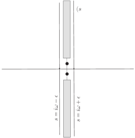
For $G\neq 0$, the self-energy as a function of frequency and momentum is in general complex, the imaginary part arises from multiparticle thresholds. When the imaginary part of the self-energy does not vanish at the value of the frequency corresponding to the dispersion relation of the free particle states, these particles can decay and no longer appear as asymptotic states. The poles in the Green’s function move off the physical sheet into a higher Riemann sheet, the particles now become resonances.

Single particle states correspond to true poles of the propagator (Green’s function) in the physical sheet, which are necessarily away from the multiparticle thresholds. This case is depicted in fig. (2).

Figure 2: Bromwich contour in s-plane, the shaded region denotes the cut discontinuity from multiparticle thresholds across the imaginary axis, the filled circles represent the single particle poles.

Let us consider the Green’s function in the flavor basis eqn. (105). The single particle poles are determined by the poles of $\mathcal{S}(k;s)$ on the imaginary axis away from the multiparticle cuts. These are determined by the roots of the following equations

$$\Omega^{2}_{1}(k) = \overline{\omega}^{\,2}(k)+\overline{\Sigma}_{R}(k;\Omega_{1}(k))-\frac{\delta M^{2}}{2}\Big{[}\big{(}\cos 2\theta-\Delta_{R}(k;\Omega_{1}(k))\big{)}^{2}+\big{(}\sin 2\theta\big{)}^{2}\Big{]}^{\frac{1}{2}}$$ (135)

$$\Omega^{2}_{2}(k) = \overline{\omega}^{\,2}(k)+\overline{\Sigma}_{R}(k;\Omega_{2}(k))+\frac{\delta M^{2}}{2}\Big{[}\big{(}\cos 2\theta-\Delta_{R}(k;\Omega_{2}(k))\big{)}^{2}+\big{(}\sin 2\theta\big{)}^{2}\Big{]}^{\frac{1}{2}}$$ (136)

along with the conditions

$$\overline{\Sigma}_{I}(k;\Omega_{1,2}(k))=0~{}~{};~{}~{}\Delta_{I}(k;\Omega_{1,2}(k))=0$$ (137)

where the subscripts $R,I$ refer to the real and imaginary parts respectively. Evaluating the residues at the single particle poles and using that the real and imaginary parts of the self-energies are even and odd functions of frequency respectively, we find

$$G_{f}(k;t)=Z^{(1)}_{k}\,\frac{\sin(\Omega_{1}(k)t)}{\Omega_{1}(k)}~{}~{}\mathds{R}^{(1)}\big{(}\theta^{(1)}_{m}(k)\big{)}+Z^{(2)}_{k}\,\frac{\sin(\Omega_{2}(k)t)}{\Omega_{2}(k)}~{}~{}\mathds{R}^{(2)}\big{(}\theta^{(2)}_{m}(k)\big{)}+G_{f,cut}(t)$$ (138)

where $G_{f,cut}(t)$ is the contribution from the multiparticle cut, the matrices $\mathds{R}^{(1,2)}$ are given by (119,120) and $\theta^{1,2}_{m}(k)$ are the mixing angles in the medium

$$\cos 2\theta^{i}_{m}(k)=\frac{\cos 2\theta-\Delta_{R}(\Omega_{i}(k))}{\Big{[}\big{(}\cos 2\theta-\Delta_{R}(k;\Omega_{i}(k))\big{)}^{2}+\big{(}\sin 2\theta\big{)}^{2}\Big{]}^{\frac{1}{2}}}~{}~{};~{}~{}\sin 2\theta^{i}_{m}(k)=\frac{\sin 2\theta}{\Big{[}\big{(}\cos 2\theta-\Delta_{R}(k;\Omega_{i}(k))\big{)}^{2}+\big{(}\sin 2\theta\big{)}^{2}\Big{]}^{\frac{1}{2}}}\,.$$ (139)

for $i=1,2$. The wave function renormalization constants are given by

$$Z^{(i)}_{k}=\Bigg{[}1-\frac{1}{2\omega}\Big{(}\overline{\Sigma}^{{}^{\prime}}_{R}(k;\omega)-(-1)^{i}\frac{\delta M^{2}}{2}\cos 2\theta^{i}_{m}(k)\Delta^{{}^{\prime}}_{R}(k;\omega)\Big{)}\Bigg{]}^{-1}_{\omega=\Omega^{i}(k)}$$ (140)

where the prime stands for derivative with respect to $\omega$. At asymptotically long time the contribution from the cut $G_{f,cut}(t)\sim t^{-\alpha}$ where $\alpha$ is determined by the behavior of the self-energy at thresholdthreshold ; maiani .

In perturbation theory and in the limit $\overline{\omega}(k)^{\,2}\gg|\delta M^{2}|$ the dispersion relations (135,136) can be solved by writing

$$\pm\Omega^{i}(k)=\pm(\overline{\omega}(k)+\delta\omega_{i}(k))\,,$$ (141)

we find

$$\delta\omega_{i}(k)=\frac{\overline{\Sigma}_{R}(k;\overline{\omega}(k))}{2\,\overline{\omega}(k)}+(-1)^{i}~{}~{}\frac{\delta M^{2}}{4\,\overline{\omega}(k)}\,\overline{\varrho}(k)$$ (142)

where we defined

$$\varrho(k;\omega)=\Bigg{[}(\cos 2\theta-\Delta_{R}(k;\omega))^{2}+(\sin 2\theta)^{2}\Bigg{]}^{\frac{1}{2}}$$ (143)

and the shorthand

$$\overline{\varrho}(k)=\varrho(k;\omega=\overline{\omega}(k))\,.$$ (144)

To leading order in the perturbative expansion and in $\delta M^{2}/\overline{\omega}^{\,2}(k)$ we find $\theta^{(1)}_{m}(k)=\theta^{(2)}_{m}(k)=\theta_{m}(k)$. Gathering these results, we find the dispersion relations and mixing angles in the medium to be given by the following relations,

$$\Omega_{1}(k) = \overline{\omega}(k)+\frac{\overline{\Sigma}_{R}(k;\overline{\omega}(k))}{2\,\overline{\omega}(k)}-\frac{\delta M^{2}}{4\,\overline{\omega}(k)}\,\overline{\varrho}(k)$$ (145)

$$\Omega_{2}(k) = \overline{\omega}(k)+\frac{\overline{\Sigma}_{R}(k;\overline{\omega}(k))}{2\,\overline{\omega}(k)}+\frac{\delta M^{2}}{4\,\overline{\omega}(k)}\,\overline{\varrho}(k)\,,$$ (146)

and

$$\cos 2\theta_{m}(k)=\frac{\cos 2\theta-\Delta_{R}(k;\overline{\omega}(k))}{\Big{[}\big{(}\cos 2\theta-\Delta_{R}(k;\overline{\omega}(k))\big{)}^{2}+\big{(}\sin 2\theta\big{)}^{2}\Big{]}^{\frac{1}{2}}}~{}~{};~{}~{}\sin 2\theta_{m}(k)=\frac{\sin 2\theta}{\Big{[}\big{(}\cos 2\theta-\Delta_{R}(k;\overline{\omega}(k))\big{)}^{2}+\big{(}\sin 2\theta\big{)}^{2}\Big{]}^{\frac{1}{2}}}\,.$$ (147)

These dispersion relations and mixing angles have exactly the same form as those obtained in the field theoretical studies of neutrino mixing in a mediumnotzold ; boyho .

V.3 Quasiparticles and relaxation.

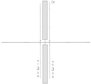
Even a particle that is stable in the vacuum acquires a width in the medium through several processes, such as collisional broadening or Landau dampingkapusta . In this case there are no isolated poles in the Green’s function in the physical sheet, the poles move off the imaginary axis in the complex $s-$plane on to a second or higher Riemann sheet. The Green’s function now features branch cut discontinuities across the imaginary axis perhaps with isolated regions of analyticity. The inverse Laplace transform is now carried out by wrapping around the imaginary axis as shown in fig. (3), and the real time Green’s function is given by

$$G_{\alpha\beta}(k;t)=\frac{i}{\pi}\int_{-\infty}^{\infty}d\omega\,e^{i\omega t}~{}~{}\mathrm{Im}\widetilde{G}_{\alpha\beta}(k;s=i\omega+\epsilon)$$ (148)

Under the validity of perturbation theory, when the inequality (116) is fulfilled we consistently keep terms up to $\mathcal{O}(G^{2})$ and find the imaginary part to be given by the following expression

$$\mathrm{Im}\widetilde{G}(k;s=i\omega+\epsilon)=\frac{-\mathds{A}(D_{-}\gamma_{+}+D_{+}\gamma_{-})+\mathds{B}(D_{+}D_{-}-\gamma_{+}\gamma_{-})}{(D^{2}_{+}+\gamma^{2}_{+})(D^{2}_{-}+\gamma^{2}_{-})}$$ (149)

where we have introduced

$$D_{\pm}(k;\omega) = -\omega^{2}+\overline{\omega}^{\,2}_{k}+\overline{\Sigma}_{R}(k;\omega)~{}\mp\frac{1}{2}\delta M^{2}\varrho(k;\omega)$$ (150)

$$\gamma_{\pm}(k;\omega) = \frac{1}{2}\left(1\pm\cos 2\theta_{m}(\omega,k)\right)\,\Sigma_{I,ee}(k;\omega)+\frac{1}{2}\left(1\mp\cos 2\theta_{m}(\omega,k)\right)\,\Sigma_{I,\mu\mu}(k;\omega)$$ (151)

$\Sigma_{R,I}$ are the real and imaginary parts of the self energy respectively, with

$$\Delta_{R}(k;\omega)=\frac{1}{\delta M^{2}}\left[\Sigma_{R,ee}(k;\omega)+V_{ee}-\Sigma_{R,\mu\mu}(k;\omega)-V_{\mu\mu}\right]\,,$$ (152)

and

$$\mathds{A}(k;\omega)=\left[-\omega^{2}+\overline{\omega}^{\,2}_{k}+\overline{\Sigma}_{R}(k;\omega)\mathds{1}\right]+\frac{\delta M^{2}}{2}\left(\begin{array}[]{cc}\cos 2\theta-\Delta_{R}(k;\omega)&-\sin 2\theta\\ -\sin 2\theta&-\cos 2\theta+\Delta_{R}(k;\omega)\end{array}\right)\;,$$ (153)

$$\mathds{B}(k;\omega)=\left(\begin{array}[]{cc}\Sigma_{I,\mu\mu}(k;\omega)&0\\ 0&\Sigma_{I,ee}(k;\omega)\\ \end{array}\right)\,.$$ (154)

The denominator in (149) features complex zeroes for

$$D_{\pm}(k;\omega)+\gamma_{\pm}(k;\omega)=0\,.$$ (155)

Near these zeroes $\mathrm{Im}\widetilde{G}(k;s=i\omega+\epsilon)$ has the typical Breit-Wigner form for resonances. The dynamical evolution at long times is dominated by the complex poles in the upper half $\omega-$ plane associated with these resonances. In perturbation theory the complex poles of $\mathrm{Im}\widetilde{G}(k;s=i\omega+\epsilon)$ occur at

$$\omega=\pm\Omega_{1}(k)+i\frac{\Gamma_{1}(k)}{2}$$ (156)

and

$$\omega=\pm\Omega_{2}(k)+i\frac{\Gamma_{2}(k)}{2}$$ (157)

where $\Omega_{1,2}(k)$ are given by (135,136) and

$$\frac{\Gamma_{1}(k)}{2}=\frac{\gamma_{+}(k,\Omega_{1}(k))}{2\,\Omega_{1}(k)}\approx\frac{\gamma_{+}(k,\overline{\omega}(k))}{2\,\overline{\omega}(k)}~{}~{};~{}~{}\frac{\Gamma_{2}(k)}{2}=\frac{\gamma_{-}(k,\Omega_{2}(k))}{2\,\Omega_{2}(k)}\approx\frac{\gamma_{-}(k,\overline{\omega}(k))}{2\,\overline{\omega}(k)}$$ (158)

These relaxation rates can be written in an illuminating manner

$$\Gamma_{1}(k) = \Gamma_{ee}(k)\cos^{2}\theta_{m}(k)+\Gamma_{\mu\mu}(k)\sin^{2}\theta_{m}(k)$$ (159)

$$\Gamma_{2}(k) = \Gamma_{\mu\mu}(k)\cos^{2}\theta_{m}(k)+\Gamma_{ee}(k)\sin^{2}\theta_{m}(k)$$ (160)

where

$$\Gamma_{\alpha\alpha}(k)=\frac{\Sigma_{I,\alpha\alpha}(k;\overline{\omega}(k))}{\overline{\omega}(k)}$$ (161)

are the relaxation rates of the flavor fields in absence of mixing. These relaxation rates are similar to those proposed within the context of flavor conversions in supernovaeraffsigl , or active-sterile oscillationsaba ; foot ; dibari .

Figure 3: Bromwich contour in s-plane, the shaded region denotes the cut discontinuity from multiparticle thresholds across the imaginary axis.

We carry out the frequency integral in (148) by approximating the integrand as a sum of two Breit-Wigner Lorentzians near $\omega=\pm\Omega_{1,2}(k)$ with the following result in the flavor basis,

$$G_{f}(k;t)= Z^{(1)}_{k}\,e^{-\frac{\Gamma_{1}(k)}{2}t}\,\Bigg{[}\frac{\sin(\Omega_{1}(k)t)}{{\Omega_{1}(k)}}\,\mathds{R}^{(1)}(\theta_{m}(k))-\frac{\widetilde{\gamma}(k)}{2}\,\frac{\cos(\Omega_{1}(k)t)}{\Omega_{1}(k)}\,\mathds{R}^{(3)}(\theta_{m}(k))\Bigg{]}+$$ (162)

$$Z^{(2)}_{k}\,e^{-\frac{\Gamma_{2}(k)}{2}t}\,\Bigg{[}\frac{\sin(\Omega_{2}(k)t)}{\Omega_{2}(k)}\,\mathds{R}^{(2)}(\theta_{m}(k))+\frac{\widetilde{\gamma}(k)}{2}\,\frac{\cos(\Omega_{2}(k)t)}{\Omega_{2}(k)}\,\mathds{R}^{(3)}(\theta_{m}(k))\Bigg{]}$$

where again we have used the approximation $|\delta M^{2}|\ll\overline{\omega}^{\,2}(k)$ and introduced

$$\mathds{R}^{(3)}(\theta)=\sin 2\theta~{}~{}\left(\begin{array}[]{cc}\sin 2\theta&\cos 2\theta\\ \cos 2\theta&-\sin 2\theta\\ \end{array}\right)=\sin 2\theta\,U(\theta)~{}\left(\begin{array}[]{cc}0&1\\ 1&0\\ \end{array}\right)~{}U^{-1}(\theta)$$ (163)

and

$$\widetilde{\gamma}(k)=\frac{\Sigma_{I,ee}(k;\overline{\omega}(k)-\Sigma_{I,\mu\mu}(k;\overline{\omega}(k))}{\delta M^{2}\,\overline{\varrho}(k)}\,.$$ (164)

Under the assumption that $\Sigma_{R,\alpha,\alpha}\gg\Sigma_{I,\alpha,\alpha}$ it follows that $\widetilde{\gamma}(k)\ll 1$. As in the previous section, we can approximately project the positive frequency component by choosing the initial condition (128) with $\Omega_{\alpha}=\overline{\omega}(k)$, leading to the result

$$\langle\Psi_{\alpha,\vec{k}}(t)\rangle=e^{-iW(k)t-\frac{\overline{\Gamma}(k)}{2}t} \Bigg{\{}Z^{(1)}_{k}\,e^{i\Delta\omega(k)t-\frac{\Delta\Gamma(k)}{2}t}~{}\Big{(}\mathds{R}^{(1)}(\theta_{m}(k))+i\frac{\widetilde{\gamma}(k)}{2}\,\mathds{R}^{(3)}(\theta_{m}(k))\Big{)}+$$ (165)

$$Z^{(2)}_{k}\,e^{-i\Delta\omega(k)t+\frac{\Delta\Gamma(k)}{2}t}~{}\Big{(}\mathds{R}^{(2)}_{\alpha,\beta}(\theta)-i\frac{\widetilde{\gamma}(k)}{2}\,\mathds{R}^{(3)}(\theta_{m}(k))\Big{)}+\mathcal{O}\Bigg{(}\frac{\delta M^{2}}{\overline{\omega}^{\,2}(k)}\Bigg{)}\Bigg{\}}\Psi^{0}_{\beta,\vec{k}}$$

where

$$W(k) = \overline{\omega}(k)+\frac{\overline{\Sigma}_{R}(k;\overline{\omega}(k))}{4\,\overline{\omega}(k)}$$ (166)

$$\frac{\overline{\Gamma}(k)}{2} = \frac{1}{4\overline{\omega}(k)}\,\Big{[}\Sigma_{I,ee}(k,\overline{\omega}(k)+\Sigma_{I,\mu\mu}(k,\overline{\omega}(k)\Big{]}$$ (167)

$$\Delta\omega(k) = \frac{\delta M^{2}\,\overline{\varrho}(k)}{4\,\overline{\omega}(k)}$$ (168)

$$\frac{\Delta\Gamma(k)}{2} = \frac{\cos 2\theta_{m}}{4~{}\overline{\omega}(k)}\,\Big{[}\Sigma_{I,ee}(k,\overline{\omega}(k)-\Sigma_{I,\mu\mu}(k,\overline{\omega}(k)\Big{]}$$ (169)

With the initial condition (133) we now find the long time evolution of the transition probability $\Psi_{e}\rightarrow\Psi_{\mu}$

$$|\langle\Psi_{\mu,\vec{k}}(t)\rangle|^{2}\sim\frac{\sin^{2}2\theta_{m}(k)}{4}\Big{[}e^{-{\Gamma_{1}(k)}t}+e^{-{\Gamma_{2}(k)}t}-2~{}e^{-\frac{1}{2}(\Gamma_{1}(k)+\Gamma_{2}(k))t}\cos\big{(}2\Delta\omega(k)t\big{)}\Big{]}~{}\Psi^{0}_{e,\vec{k}}$$ (170)

where we have neglected perturbatively small terms by setting $Z^{(i)}\sim 1~{};~{}\widetilde{\gamma}(k)\sim 0$ in prefactors. The solution (165) can be written in the following illuminating form

$$\langle\Psi_{\alpha,\vec{k}}(t)\rangle=e^{-iW(k)t-\frac{\overline{\Gamma}(k)}{2}t}\,\mathcal{U}\big{(}\theta_{m}(k)\big{)}~{}\Bigg{(}\begin{array}[]{cc}Z^{(1)}_{k}\,e^{i\Delta\omega(k)t-\frac{\Delta\Gamma(k)}{2}t}&0\\ 0&Z^{(2)}_{k}\,e^{-i\Delta\omega(k)t+\frac{\Delta\Gamma(k)}{2}t}\\ \end{array}\Bigg{)}~{}\mathcal{U}^{-1}\big{(}\theta_{m}(k)\big{)}~{}\Psi^{0}_{\beta,\vec{k}}$$ (171)

where

$$\mathcal{U}\big{(}\theta_{m}(k)\big{)}=\Bigg{(}\begin{array}[]{cc}\cos\theta_{m}(k)\big{(}1+i\widetilde{\gamma}(k)\big{)}&\sin\theta_{m}(k)\big{(}1-i\widetilde{\gamma}(k)\big{)}\\ -\sin\theta_{m}(k)&\cos\theta_{m}(k)\\ \end{array}\Bigg{)}$$ (172)

$$\mathcal{U}^{-1}\big{(}\theta_{m}(k)\big{)}=\frac{1}{\big{(}1+i~{}\cos\theta_{m}(k)~{}\widetilde{\gamma}(k)\big{)}}\Bigg{(}\begin{array}[]{cc}\cos\theta_{m}(k)&-\sin\theta_{m}(k)\big{(}1-i\widetilde{\gamma}(k)\big{)}\\ -\sin\theta_{m}(k)&\cos\theta_{m}(k)\big{(}1+i\widetilde{\gamma}(k)\big{)}\\ \end{array}\Bigg{)}$$ (173)

Obviously the matrix $\mathcal{U}$ is not unitary.

V.4 Long time dynamics: Weisskopf-Wigner Hamiltonian

A phenomenological description of the dynamics of mixing and decay for neutral flavored mesons, for example $K_{0}\overline{K}_{0}~{};~{}B_{0}\overline{B}_{0}$ relies on the Weisskopf-Wigner (WW) approximationWW1 . In this approximation the time evolution of states is determined by a non-hermitian Hamiltonian that includes in a phenomenological manner the exponential relaxation associated with the decay of the neutral mesons. This approach has received revived attention recently with the possibility of observation of quantum mechanical coherence effects, in particular CP-violation in current experiments with neutral mesonsWW2 . In ref.WW3 a field theoretical analysis of the (WW) approximation has been provided for the $K_{0}\overline{K}_{0}$ system.

The form of the solution (171) suggests that a (WW) approximate description of the asymptotic dynamics in terms of a non-hermitian Hamiltonian is available. To achieve this formulation we separate explicitly the fast time dependence via the phase $e^{\mp i\overline{\omega}(k)t}$ for the positive and negative frequency components, writing

$$\Psi_{\vec{k}}(t)=e^{-i\overline{\omega}(k)t}~{}\Psi^{+}_{\vec{k}}(t)+e^{i\overline{\omega}(k)t}~{}\Psi^{-}_{\vec{k}}(t)$$ (174)

where $\Psi^{\pm}_{\vec{k}}(t)$ the amplitudes of the flavor vectors that evolve slowly in time. The solution for the positive frequency component (165) follows from the time evolution of the slow component determined by

$$i\frac{d}{dt}\Psi^{+}_{\vec{k}}(t)=\mathcal{H}_{w}\Psi^{+}_{\vec{k}}(t)$$ (175)

where the effective non-hermitian Hamiltonian $\mathcal{H}$ is given by

$$\mathcal{H}_{w}=\frac{\delta M^{2}}{4\,\overline{\omega}(k)}\Big{(}\begin{array}[]{cc}-\cos 2\theta&\sin 2\theta\\ \sin 2\theta&\cos 2\theta\\ \end{array}\Big{)}+\frac{\Sigma_{R}(k;\overline{\omega}(k))+\mathds{V}}{2\,\overline{\omega}(k)}-i\,\frac{\Sigma_{I}(k;\overline{\omega}(k))}{2\,\overline{\omega}(k)}$$ (176)

with

$$\Sigma_{R}(k;\overline{\omega}(k))+\mathds{V} = \Bigg{(}\begin{array}[]{cc}\Sigma_{R,ee}(k;\overline{\omega}(k))+V_{ee}&0\\ 0&\Sigma_{R,\mu\mu}(k;\overline{\omega}(k))+V_{\mu\mu}\\ \end{array}\Bigg{)}$$ (179)

$$\Sigma_{I}(k;\overline{\omega}(k)) = \Bigg{(}\begin{array}[]{cc}\Sigma_{I,ee}(k;\overline{\omega}(k))&0\\ 0&\Sigma_{I,\mu\mu}(k;\overline{\omega}(k))\\ \end{array}\Bigg{)}$$ (182)

The (WW) Hamiltonian $\mathcal{H}_{w}$ can be written as

$$\mathcal{H}_{w}=\Big{\{}\frac{\overline{\Sigma}_{R}(k;\overline{\omega}(k))}{4\,\overline{\omega}(k)}-i\frac{\overline{\Gamma}(k)}{2}\Big{\}}\mathds{1}+\frac{\delta M^{2}~{}\overline{\varrho}(k)}{4~{}\overline{\omega}(k)}\,\Bigg{(}\begin{array}[]{cc}-(\cos 2\theta_{m}(k)+i\widetilde{\gamma}(k))&\sin 2\theta_{m}(k)\\ \sin 2\theta_{m}(k)&(\cos 2\theta_{m}(k)+i\widetilde{\gamma}(k))\\ \end{array}\Bigg{)}$$ (183)

where we have used the definitions given in equations (143,144,147,164,167). It is straightforward to confirm that the Wigner-Weisskopf Hamiltonian can be written as

$$\mathcal{H}_{w}=\mathcal{U}(\theta_{m}(k))~{}\Bigg{(}\begin{array}[]{cc}\lambda_{-}(k)&0\\ 0&\lambda_{+}(k)\\ \end{array}\Bigg{)}~{}\mathcal{U}^{-1}(\theta_{m}(k))$$ (184)

where $\mathcal{U}(\theta_{m}(k))$ is given in (172) and using the definitions given in eqn. (166-169) the complex eigenvalues are

$$\lambda_{\mp}(k)=W(k)-\overline{\omega}(k)-i\frac{\overline{\Gamma}(k)}{2}\mp\left(\Delta\omega(k)+i\frac{\Delta\Gamma(k)}{2}\right)$$ (185)

The solution of the effective equation for the slow amplitudes (175) coincides with the long time dynamics given by (165) when the wave function renormalization constants are approximated as $Z^{(i)}_{\vec{k}}\sim 1$. Therefore the (WW) description of the time evolution based on the non-hermitian Hamiltonian $\mathcal{H}_{w}$ (176) effectively describes the evolution of flavor multiplets under the following approximations:

• Only the long-time dynamics can be extracted from the Weisskopf-Wigner Hamiltonian.

• The validity of the perturbative expansion, and of the condition $\delta M^{2}\ll\overline{\omega}(k)^{2}$.

• Wavefunction renormalization corrections are neglected $Z^{(i)}\sim 1$ and only leading order corrections of order $\widetilde{\gamma}(k)$ are included.

While the Weisskopf-Wigner effective description describes the relaxation of the flavor fields, it misses the stochastic noise from the bath, therefore, it does not reliably describe the approach to equilibrium.

VI Equilibration: effective Hamiltonian in the medium

As discussed in section III.1 we study equilibration by focusing on the asymptotic long time behavior of the one-body density matrix or equal time correlation function, namely

$$\lim_{t\rightarrow\infty}\,\langle\Psi_{\alpha,\vec{k}}(t)\Psi_{\beta,-\vec{k}}(t)\rangle\,.$$ (186)

In particular we seek to understand which basis diagonalizes the equilibrium density matrix.

Consider general initial conditions $\Psi^{0}\neq 0$ and $\Pi^{0}\neq 0$, in which case the flavor field $\Psi_{\alpha,\vec{k}}(t)$ is given by Eq. (104) with $G_{f}(k;t)$ given by eqn. (162). For $t\gg\Gamma^{-1}_{1,2}$, the first two contributions to (104) which depend on the initial conditions fall-off exponentially as $e^{-\frac{\Gamma_{1,2}}{2}t}$ and only the last term, the convolution with the noise, survives at asymptotically long time, indicating that the equilibrium state is insensitive to the initial conditions as it must be.

To leading order in the perturbative expansion in $G$, and in the limit $\delta M^{2}/\overline{\omega}^{\,2}(k)\ll 1$, we can approximate $\theta^{(1)}_{m}(k)\approx\theta^{(2)}_{m}(k)=\theta_{m}(k)$, where the effective mixing angle in the medium $\theta_{m}(k)$ is determined by the relations (147). Similarly we can approximate the wave function renormalization constants as $Z^{(1)}(k)\approx Z^{(2)}(k)=Z(k)$ with

$$Z(k)=\Bigg{[}1-\frac{1}{2\omega}\Big{(}\overline{\Sigma}^{{}^{\prime}}_{R}(k;\omega)-(-1)^{i}\frac{\delta M^{2}}{2}\cos 2\theta_{m}(k)\Delta^{{}^{\prime}}_{R}(k;\omega)\Big{)}\Bigg{]}^{-1}_{\omega=\overline{\omega}(k)}$$ (187)

where the prime stands for derivative with respect to $\omega$. Thus, $G_{f}(k;t)$ and $G_{m}(k;t)$ are related by

$$G_{f}(k;t)\approx Z(k)\,U(\theta_{m})\,G_{m}(k;t)\,U^{-1}(\theta_{m})$$ (188)

where $G_{m}(k;t)$ is given by

$$G_{m}(k;t)= \Bigg{(}\begin{array}[]{cc}\frac{\sin(\Omega_{1}(k)t)}{\Omega_{1}(k)}~{}e^{-\frac{\Gamma_{1}(k)}{2}t}&0\\ 0&\frac{\sin(\Omega_{2}(k)t)}{\Omega_{2}(k)}~{}e^{-\frac{\Gamma_{2}(k)}{2}t}\end{array}\Bigg{)}+$$ (194)

$$\frac{\widetilde{\gamma}(k)}{2}~{}\sin 2\theta_{m}(k)\left[e^{-\frac{\Gamma_{2}(k)}{2}t}\frac{\cos(\Omega_{2}(k)t)}{\Omega_{2}(k)}-e^{-\frac{\Gamma_{1}(k)}{2}t}\frac{\cos(\Omega_{1}(k)t)}{\Omega_{1}(k)}\right]\left(\begin{array}[]{cc}0&1\\ 1&0\\ \end{array}\right)\,.$$

It is useful to define the quantities $h_{m}(t,\omega)$ and $\widetilde{\xi}_{\beta,\vec{k}}(\omega)$ as follows

$$h_{m}(t,\omega)=\int_{0}^{t}\,e^{-i\omega t^{\prime}}\,G_{m}(k;t)\,dt^{\prime}$$ (195)

and

$$\xi_{\beta,\vec{k}}(t-t^{\prime})=\int_{-\infty}^{+\infty}\,e^{i\omega(t-t^{\prime})}\,\widetilde{\xi}_{\beta,\vec{k}}(\omega)\,d\omega,$$ (196)

with the noise average in the flavor basis given by

$$\langle\langle\,\widetilde{\xi}_{\rho,\vec{k}}(\omega)\,\widetilde{\xi}_{\sigma,-\vec{k}}(\omega^{\prime})\,\rangle\rangle=\widetilde{{\mathcal{K}}}_{\rho\sigma}(k;\omega)\delta(\omega+\omega^{\prime})=\mathrm{Im}\widetilde{\Sigma}^{R}_{\rho\sigma}(k;\omega)\coth\left(\frac{\beta\omega}{2}\right)\delta(\omega+\omega^{\prime})\,.$$ (197)

We find convenient to introduce

$$\widetilde{{\mathcal{K}}}_{m}(k;\omega)=U^{-1}(\theta_{m})\,\widetilde{{\mathcal{K}}}(k;\omega)\,U(\theta_{m})\,.$$ (198)

The approach to equilibrium for $t>>\Gamma^{-1}_{1,2}$ can be established from the unequal time two-point correlation function, given by

$$\lim_{t,t^{\prime}\rightarrow\infty}\,\langle\Psi_{\alpha,\vec{k}}(t)\Psi_{\beta,-\vec{k}}(t^{\prime})\rangle=Z^{2}(k)U(\theta_{m})\Bigg{\{}\int_{-\infty}^{+\infty}\,d\omega~{}~{}e^{i\omega(t-t^{\prime})}~{}~{}h_{m}(\infty,\omega)\,\widetilde{{\mathcal{K}}}_{m}(k;\omega)\,h_{m}(\infty,-\omega)\Bigg{\}}U^{-1}(\theta_{m})$$ (199)

where we have taken the upper limit $t\rightarrow\infty$ in (196). The fact that the correlation function becomes a function of the time difference, namely time translational invariant, indicates that the density matrix commutes with the total Hamiltonian in the long time limit. The one-body density matrix is obtained from (199) in the coincidence limit $t=t^{\prime}$.

Performing the integration over $\omega$, we obtain after a lengthy but straightforward calculation

$$\lim_{t\rightarrow\infty}\,\langle\Psi_{\alpha,\vec{k}}(t)\Psi_{\beta,-\vec{k}}(t)\rangle=Z^{2}(k)\,U(\theta_{m})\,\left(\begin{array}[]{cc}\Lambda_{11}(k)&\Lambda_{12}(k)\\ \Lambda_{21}(k)&\Lambda_{22}(k)\\ \end{array}\right)\,U^{-1}(\theta_{m});$$ (202)

wherein

$$\Lambda_{11}(k)=\frac{1}{2\,\Omega_{1}(k)}\coth\left(\frac{\beta\Omega_{1}(k)}{2}\right)~{};~{}~{}\Lambda_{22}(k)=\frac{1}{2\,\Omega_{2}(k)}\coth\left(\frac{\beta\Omega_{2}(k)}{2}\right),$$ (203)

and to the leading order of $\delta M^{2}/\overline{\omega(k)}^{\,2}\ll 1$, we find $\Lambda_{21}=\Lambda_{12}(\Omega_{1}\rightarrow\Omega_{2})$ where

$$\Lambda_{12}(k) = \frac{1}{2\,\Omega_{1}(k)}\coth\left(\frac{\beta\Omega_{1}(k)}{2}\right)\sin 2\theta_{m}(k)\;\frac{\widetilde{\gamma}(k)\,\eta(k)}{1+\left(\,\eta(k)\,\right)^{2}}~{};~{}~{}\eta(k)=\frac{2\Omega_{1}(k)\left(\,\Gamma_{1}(k)+\Gamma_{2}(k)\,\right)}{\delta M^{2}\overline{\varrho}(k)}.$$ (204)

Since $\widetilde{\gamma}(k)\ll 1$, it is obvious that $\Lambda_{12}(k)$ and $\Lambda_{21}(k)$ are perturbatively small compared with $\Lambda_{11}(k)$ and $\Lambda_{22}(k)$, in either case $\eta(k)\gg 1$ or $\eta(k)\ll 1$. The asymptotic one-body density matrix (76) then becomes

$$\rho_{\alpha,\beta}(k;\infty)=U(\theta_{m})\,\left(\begin{array}[]{cc}\frac{Z}{2\,\Omega_{1}(k)}\coth\left(\frac{\beta\Omega_{1}(k)}{2}\right)&\epsilon\\ \epsilon&\frac{Z}{2\,\Omega_{2}(k)}\coth\left(\frac{\beta\Omega_{2}(k)}{2}\right)\\ \end{array}\right)\,U^{-1}(\theta_{m})~{}~{};~{}~{}\epsilon\lesssim\mathcal{O}(G^{2})$$ (205)

where we neglected corrections of $\mathcal{O}(G^{2})$ in the diagonal matrix elements.

Neglecting the perturbative off-diagonal corrections, the one-body density matrix commutes with the effective Hamiltonian in the medium which in the flavor basis is given by

$$H_{eff}(k)=\overline{\omega}(k)\Bigg{(}\begin{array}[]{cc}1&0\\ 0&1\end{array}\Bigg{)}+\frac{\delta M^{2}}{4\,\overline{\omega}(k)}\Bigg{(}\begin{array}[]{cc}-\cos 2\theta&\sin 2\theta\\ \sin 2\theta&\cos 2\theta\\ \end{array}\Bigg{)}+\frac{1}{2\overline{\omega}(k)}\,\Bigg{(}\begin{array}[]{cc}\Sigma_{R,ee}(k;\overline{\omega}(k))+V_{ee}&0\\ 0&\Sigma_{R,\mu\mu}(k;\overline{\omega}(k))+V_{\mu\mu}\\ \end{array}\Bigg{)}$$ (206)

this effective in-medium Hamiltonian can be written in a more illuminating form

$$H_{eff}(k)=U(\theta_{m})\,\Bigg{(}\begin{array}[]{cc}\Omega_{1}(k)&0\\ 0&\Omega_{2}(k)\\ \end{array}\Bigg{)}\,U^{-1}(\theta_{m})$$ (207)

where $\Omega_{1,2}(k)$ are the correct propagation frequencies in the medium given by eqn. (145,146).

This effective Hamiltonian includes the radiative corrections in the medium via the flavor diagonal self-energies (forward scattering) and apart from the term proportional to the identity is identified with the real part of the Weisskopf-Wigner Hamiltonian $\mathcal{H}_{w}$ given by eqn. (176). This form highlights that the off-diagonal elements of the one-body density matrix in the basis of eigenstates of the effective Hamiltonian in the medium are perturbatively small. The unitary transformation $U(\theta_{m})$ relates the flavor fields to the fields in the basis of the effective Hamiltonian in the medium.

Comparing this result to the free field case in thermal equilibrium, where the one body density matrix in the flavor basis is given by eqn. (79), it becomes clear that in the long time limit equilibration is achieved and the one-body density matrix is nearly diagonal in the basis of the eigenstates of the effective Hamiltonian in the medium (206) with the diagonal elements determined by the distribution function of these eigenstates.

This means that within the realm of validity of perturbation theory, the equilibrium correlation function is nearly diagonal in the basis of the effective Hamiltonian in the medium. This result confirms the arguments advanced in chargedlepton . Since the effective action is quadratic in the “neutrino fields” higher correlation functions are obtained as Wick contractions of the two point correlators, hence the fact that the two point correlation function and consequently the one-body density matrix are diagonal in the basis of the eigenstates of the effective Hamiltonian in the medium guarantee that all higher correlation functions are also diagonal in this basis.

VI.1 On “sterile neutrinos”

The results obtained in the previous sections apply to the case of two “flavored neutrinos” both in interaction with the bath. However, these results can be simply extrapolated to the case of one “active” and one “sterile” neutrino that mix via a mass matrix that is off-diagonal in the flavor basis. By definition a “sterile” neutrino does not interact with hadrons, quarks or charged leptons, therefore for this species there are no radiative corrections. Consider for example that the “muon neutrino” represented by $\phi_{\mu}$ does not couple to the bath, but it does couple to the “electron neutrino” solely through the mixing in the mass matrix. Since the interaction is diagonal in the flavor basis, the decoupling of this “sterile neutrino” can be accounted for simply by imposing the following “sterility conditions” for the matter potential $\mathds{V}$ and the self energies

$$V_{\mu\mu}\equiv 0~{};~{}\Sigma_{R,\mu\mu}\equiv 0~{};~{}\Sigma_{I,\mu\mu}\equiv 0\;.$$ (208)

All of the results obtained above for the dispersion relations and relaxation rates apply to this case by simply imposing these “sterility conditions”. In particular it follows that

$$\Gamma_{1}(k)=\Gamma_{ee}(k)\cos^{2}\theta_{m}(k)~{};~{}\Gamma_{2}(k)=\Gamma_{ee}\sin^{2}\theta_{m}(k)$$ (209)

where $\Gamma_{ee}(k)$ is the relaxation rate of the active neutrino in absence of mixing. This result highlights that in the limit $\theta\rightarrow 0$ the in-medium eigenstate labeled “2” is seen to correspond to the sterile state, because in the absence of mixing this state does not acquire a width. However, for non-vanishing vacuum mixing angle, the “sterile neutrino” nonetheless equilibrates with the bath as a consequence of the “active-sterile” mixing, which effectively induces a coupling between the “sterile” and the bathdm ; aba ; foot ; raffsigl ; dibari . The result for $\Gamma_{2}(k)$, namely the relaxation rate of the “sterile” neutrino is of the same form as that proposed in refs. dm ; aba ; foot ; raffsigl ; dibari . The result for the “sterile” rate $\Gamma_{2}(k)$ compares to those in these references in the limit in which perturbation theory is valid, namely $\Sigma_{ee}(k)/\delta M^{2}\overline{\varrho}(k)\ll 1$ since the denominator in this ratio is proportional to the oscillation frequency in the medium.

VII Summary of results and conclusions

In this article we studied the non-equilibrium dynamics of mixing, oscillations and equilibration in a model field theory that bears all of the relevant features of the standard model of neutrinos augmented by a mass matrix off diagonal in the flavor basis. To avoid the complications associated with the spinor nature of the neutrino fields, we studied an interacting model of flavored neutral mesons. Two species of flavored neutral mesons play the role of two flavors of neutrinos, these are coupled to other mesons which play the role of hadrons or quarks and charged leptons, via flavor diagonal interactions that model charged currents in the standard model. These latter meson fields are taken to describe a bath in thermal equilibrium, and the meson-neutrino fields are taken to be the “system”. We obtain a reduced density matrix and the non-equilibrium effective action for the “neutrinos” by integrating out the bath degrees of freedom up to second order in the coupling in the full time-evolved density matrix.

The non-equilibrium effective action yields all the information on the particle and quasiparticle modes in the medium, and the approach to equilibrium.

Summary of results:

• We obtain the dispersion relations, mixing angles and relaxation rates of the two quasiparticle modes in the medium. The dispersion relations and mixing angles are of the same form as those obtained for neutrinos in a mediumnotzold ; boyho .

• The relaxation rates are found to be

  $$\Gamma_{1}(k) = \Gamma_{ee}(k)\cos^{2}\theta_{m}(k)+\Gamma_{\mu\mu}(k)\sin^{2}\theta_{m}(k)$$ (210)

  $$\Gamma_{2}(k) = \Gamma_{\mu\mu}(k)\cos^{2}\theta_{m}(k)+\Gamma_{ee}(k)\sin^{2}\theta_{m}(k)$$ (211)

  where

  $$\Gamma_{\alpha\alpha}(k)=\frac{\Sigma_{I,\alpha\alpha}(k;\overline{\omega}(k))}{\overline{\omega}(k)}$$ (212)

  are the relaxation rates of the flavor fields in absence of mixing and $\Sigma_{I,\alpha,\alpha}$ are the imaginary parts of the “neutrino” self energy which is diagonal in the flavor basis. These relaxation rates are similar in form to those proposed in refs.raffsigl ; aba ; foot ; dibari , within the context of active-sterile conversion or flavor conversion in supernovae.

• The long time dynamics is approximately described by an effective Weisskopf-Wigner approximation with a non-hermitian Hamiltonian. The real part includes the “index of refraction” and the renormalization of the frequencies and the imaginary part is determined by the absorptive part of the second order self-energy and describes the relaxation. While this (WW) approximation describes mixing, oscillations and relaxation, it does not capture the dynamics of equilibration.

• For time $t>>\Gamma^{-1}_{1,2}$ the two point function of the neutrino fields becomes time translational invariant reflecting the approach to equilibrium. The asymptotic long time limit of the one-body density matrix reveals that the density matrix is nearly diagonal in the basis of eigenstates of an effective Hamiltonian in the medium (206) with perturbatively small off-diagonal corrections in this basis. The diagonal components in this basis are determined by the distribution function of these eigenstates.

• “Sterile” neutrinos: these results apply to the case in which only one of the flavored neutrinos is “active” but the other is “sterile”. Consider for example that the “muon neutrino” is sterile in the sense that it does not couple to the bath. This sterile degree of freedom is thus identified with the in medium eigenstate “2” because in the absence of mixing $\theta=0$ its dynamics is completely free. The “sterility” condition corresponds to setting the matter potential $V_{\mu\mu}=0$ and the self-energy $\Sigma_{\mu\mu}=0$ with a concomitant change in the dispersion relations. All the results obtained above apply just the same, but with $\Gamma_{\mu\mu}(k)=0$, from which it follows that $\Gamma_{2}(k)=\Gamma_{ee}(k)\sin^{2}\theta_{m}(k)$. The final result is that “sterile” neutrinos do thermalize with the bath via “active-sterile” mixing. If the mixing angle in the medium is small, the equilibration time scale for the “sterile neutrino” is much larger than that for the “active” species, but equilibration is eventually achieved nonetheless. This result is a consequence of “active-sterile” oscillations which effectively induces an interaction of the sterile neutrino with the bathdm ; aba ; foot ; raffsigl ; dibari .

Although the meson field theory studied here describes quite generally the main features of mixing, oscillations and relaxation of neutrinos, a detailed quantitative assessment of the relaxation rates and dispersion relations do require a full calculation in the standard model. Furthermore there are several aspects of neutrino physics that are distinctly associated with their spinorial nature and cannot be inferred from this model. While only the left handed component of neutrinos couple to the weak interactions, a (Dirac) mass term couples the left to the right handed component, and through this coupling the right handed component develops a dynamical evolution. Although the coupling to the right handed component is very small in the ultrarelativistic limit, it is conceivable that non-equilibrium dynamics may lead to a substantial right handed component during long time intervals. The study of this possibility would be of importance in the early Universe because the right handed component may thereby become an “active” one that may contribute to the total number of species in equilibrium in the thermal bath thus possibly affecting the expansion history of the Universe.

Another important fermionic aspect is Pauli blocking which is relevant in the case in which neutrinos are degenerate, for example in supernovae.

These aspects will be studied elsewhere.