ROME1/1436/06

Modelling non-perturbative corrections
to bottom-quark fragmentation

Ugo Aglietti^1,2, Gennaro Corcella¹

and Giancarlo Ferrera^1,2

¹Dipartimento di Fisica, Università di Roma ‘La Sapienza’
P.le A. Moro 2, I-00185 Roma, Italy

²INFN, Sezione di Roma
P.le A. Moro 2, I-00185 Roma, Italy

We describe $B$-hadron production in $e^{+}e^{-}$ annihilation at the $Z^{0}$ pole by means of a model including non-perturbative corrections to $b$-quark fragmentation as originating, via multiple soft emissions, from an effective QCD coupling constant, which does not exhibit the Landau pole any longer and includes absorptive effects due to parton branching. We work in the framework of perturbative fragmentation functions at NLO, with NLL DGLAP evolution and NNLL large-$x$ resummation in both coefficient function and initial condition of the perturbative fragmentation function. We include hadronization corrections via the effective coupling constant in the NNLO approximation and do not add any further non-perturbative fragmentation function. As part of our model, we perform the Mellin transforms of our resummed expressions exactly. We present results on the energy distribution of $b$-flavoured hadrons, which we compare with LEP and SLD data, in both $x$- and $N$-spaces. We find that, within the theoretical uncertainties on our calculation, our model is able to reasonably reproduce the data at $x\raisebox{-3.0pt}{$\>\stackrel{{\scriptstyle<}}{{\scriptstyle\sim}}\>$}0.92$ and the first five moments of the $B$ cross section.

1 Introduction

We study $b$-quark fragmentation and $B$-hadron production in $e^{+}e^{-}$ annihilation using a model which implements power corrections via an analytic effective coupling constant. Such a model will allow us to make hadron-level predictions, directly comparable with the accurate experimental data from the SLD [1] and LEP [2, 3, 4] collaborations.

Let us describe in physical terms the process we are interested in:

$$e^{+}e^{-}\,\to\,Z^{0}\,\to\,B\,+\,X_{\bar{b}},$$ (1.1)

where $X_{\bar{b}}$ is a generic hadronic final state with a $\bar{b}$ quark. The corresponding parton-level process, assuming that an arbitrary number of gluons is radiated, reads:

$$Z^{0}\,\to\,b\,\bar{b}\to b\,\bar{b}\,g_{1}\,\dots\,g_{n}.$$ (1.2)

In the $Z^{0}$ rest frame, the $b$ and the $\bar{b}$ are initially emitted back-to-back with a large virtuality, of the order of the hard scale $Q=m_{Z}$. Then, they reduce their energy by emitting gluons, mainly of low energy or at small angle (soft or collinear radiation). As long as the virtuality of the $b$ quarks is large enough, we can neglect the $b$ and $\bar{b}$ masses. Considering, for simplicity, the case of one single emission,

$$e^{+}e^{-}\,\to\,Z^{0}(q)\,\to\,b(p_{b})\,+\,\bar{b}(p_{\bar{b}})\,+\,g(p_{g}),$$ (1.3)

and defining the energy fractions

$$x_{i}\,\equiv\,{{2p_{i}\cdot q}\over{m_{Z}^{2}}}\,=\,\frac{2E_{i}}{m_{Z}},$$ (1.4)

where $i\,=\,b,\bar{b},g$ and $x_{b}+x_{\bar{b}}+x_{g}=2$, a straightforward kinematical computation yields:

$$1-x_{b}={{x_{\bar{b}}x_{g}}\over 2}(1-\cos\theta_{\bar{b}g}),$$ (1.5)

with $\theta_{\bar{b}g}$ being the angle between the gluon and the $\bar{b}$. From Eq. (1.5), we see that collinear emission from the $\bar{b}$ ($\theta_{\bar{b}g}=0$) implies $x_{b}$=1. Likewise, by crossing $b\to\bar{b}$, one can show that collinear radiation off the $b$, i.e. $\theta_{bg}=0$, corresponds to $x_{\bar{b}}=1$. Soft-gluon radiation ($x_{g}=0$) yields $x_{b}=x_{\bar{b}}=1$. We can identify two main different mechanisms of energy loss of the $b$: a direct loss, related to soft or collinear emissions off the $b$ itself, and an indirect loss, when the gluons are radiated off the $\bar{b}$ (hard and large-angle emissions are not enhanced). The asymmetry between the $b$ and the $\bar{b}$ jets is not dynamical, but is just related to the fact that, e.g., we decided to measure the energy of the $b$, and not that of the $\bar{b}$.

When the virtuality of the $b$ has reduced to a value of the order of its mass, mass effects become substantial, and when it becomes comparable with the hadronic scale, ${\cal O}(1~{}\mathrm{GeV})$, the $b$ approaches the non-perturbative phase of its evolution. The hadronization, for example, into a $B$ meson can be described as due to the radiation of a light $q\bar{q}$ pair, and the subsequent combination of the $b$ and the $\bar{q}$ to form a $B\,=\,(b\bar{q})$ state:

$$b\,\to\,B\,+\,q.$$ (1.6)

In the process (1.6), the colour of the heavy $b$ is coherently transferred to the light $q$; we shall assume that no more radiation is emitted after the colourless hadron has been formed. The hadronization transition (1.6) is sensitive to non-perturbative power corrections $\Lambda/m_{b}$, with $\Lambda$ being the QCD scale, e.g., in the $\overline{\mbox{MS}}$ scheme. Such power corrections - for the time being - cannot be calculated from first principles, but are usually described by means of phenomenological hadronization models, such as the Kartvelishvili [5] or the Peterson [6] models, containing parameters which are to be fitted to experimental data. In Ref. [7], furthermore, non-perturbative effects in bottom fragmentation at large $x$ were described as a shape function of $m_{b}(1-x)$ and implemented using Dressed Gluon Exponentiation [8].

In this paper, we shall follow a different approach to model power corrections to $b$-quark fragmentation. We shall assume that the transition (1.6) can be described in terms of an effective analytic coupling constant $\tilde{\alpha}_{S}$, which incorporates non-perturbative power corrections and, unlike the models above mentioned, does not present any free parameter to be fitted to data. Within our model, whenever we use $\tilde{\alpha}_{S}$ instead of the standard $\alpha_{S}$, the energy of the $b$ quark will be identified with the one of the observed $B$ meson, i.e. $E_{b}\to E_{B}$. The non-perturbative model which we shall use hereafter was already used in [9] in the context of $B$-meson decays and interesting results were found. The comparison with the data on the photon spectrum in radiative decays and on the hadron-mass distribution in semileptonic decays showed good agreement, while discrepancies were found for the purpose of the electron energy distribution.

An analogous model can be introduced for the fragmentation of a $b$ into a baryon, such as, for example, a hyperion $\Lambda_{b}$. The $b$ quark emits two light $u\bar{u}$ and $d\bar{d}$ pairs and combines with the $u$ and the $d$ to form the colourless $\Lambda_{b}\,=\,(bud)$:

$$b\,\to\,\Lambda_{b}\,+\,\bar{u}\,+\,\bar{d},$$ (1.7)

where the $\bar{u}\bar{d}$ system is emitted with the same colour state as the initial $b$. The process (1.7) will be also described by means of an effective coupling constant: however, there is no reason a priori to assume that the effective coupling constant for (1.7) is equal to that for (1.6).

Turning back to the parton-level process (1.2), the differential cross section has a perturbative expansion containing large logarithms of the form:

$$~{}~{}~{}~{}~{}~{}~{}~{}~{}~{}~{}~{}~{}~{}~{}~{}~{}~{}~{}~{}~{}~{}~{}~{}~{}~{}~{}~{}~{}~{}~{}~{}~{}~{}~{}~{}~{}~{}~{}~{}~{}~{}~{}~{}~{}~{}~{}~{}~{}~{}~{}~{}~{}\alpha_{S}^{n}\,\ln^{k}\frac{m_{Z}^{2}}{m_{b}^{2}}~{}~{}~{}~{}~{}~{}(n=1,2,3\cdots\infty,~{}k=1,2,\cdots,n),$$ (1.8)

which are related to collinear emissions of partons with transverse momenta ranging between scales fixed by the particle masses:

$$\alpha_{S}\,\ln\frac{m_{Z}^{2}}{m_{b}^{2}}\,=\,\alpha_{S}\,\int_{m_{b}^{2}}^{m_{Z}^{2}}\frac{dk_{\perp}^{2}}{k_{\perp}^{2}}.$$ (1.9)

At higher orders, the leading contributions, $k\,=\,n$ in Eq. (1.8), are associated with phase-space regions ordered in transverse momentum:

$$k_{\perp 1}\,>\,k_{\perp 2}\,>\cdots\,>\,k_{\perp n},$$ (1.10)

leading to integrals of the form

$$\alpha_{S}^{n}\,\int_{m_{b}^{2}}^{m_{Z}^{2}}\frac{dk_{\perp 1}^{2}}{k_{\perp 1}^{2}}\,\int_{m_{b}^{2}}^{k_{\perp 1}^{2}}\frac{dk_{\perp 2}^{2}}{k_{\perp 2}^{2}}\,\,\cdots\,\,\int_{m_{b}^{2}}^{k_{\perp n-1}^{2}}\frac{dk_{\perp n}^{2}}{k_{\perp n}^{2}}\,=\,\frac{1}{n!}\,\alpha_{S}^{n}\,\ln^{n}\frac{m_{Z}^{2}}{m_{b}^{2}}.$$ (1.11)

Hence, in the first-order cross section, the collinear logarithm exponentiates.

The $b$-quark spectrum is also affected by large logarithms

$$~{}~{}~{}~{}~{}~{}~{}~{}~{}~{}~{}~{}~{}~{}~{}~{}~{}~{}~{}~{}~{}~{}~{}~{}~{}~{}~{}~{}~{}~{}~{}~{}~{}~{}~{}~{}~{}~{}~{}\alpha_{S}^{n}\,\left[\frac{\ln^{k}(1-x)}{1-x}\right]_{+}~{}~{}~{}~{}(n=1,2\cdots,\infty,~{}k=0,1,2,\cdots,2n-1),$$ (1.12)

also called threshold logarithms, which are enhanced for $x\to 1$, i.e. for soft or collinear emission. The plus distributions in Eq. (1.12) are defined as:

$$\left[\frac{\ln^{k}(1-x)}{1-x}\right]_{+}\,\equiv\,\lim_{\epsilon\to 0^{+}}\,\left[\Theta(1-x-\epsilon)\frac{\ln^{k}(1-x)}{1-x}\,-\,\delta(1-x-\epsilon)\,\int_{0}^{1-\epsilon}\frac{\ln^{k}(1-x^{\prime})}{1-x^{\prime}}\,dx^{\prime}\right].$$ (1.13)

The contributions in (1.12) originate from the following double-logarithmic integrals:

$$\left[\frac{\ln(1-x)}{1-x}\right]_{+}\,=\,-\,\left[\int_{0}^{1}\,\int_{0}^{1}\frac{d\omega}{\omega}\frac{dt}{t}\delta(1-x-\omega t)\right]_{+},$$ (1.14)

where $\omega\,\equiv\,2E_{g}/m_{Z}$, is the normalized energy of the radiated gluon and $t\,\equiv\,2(1-\cos\theta)\simeq\theta^{2}$, with $\theta$ being the emission angle. The $\delta$-function contains a typical kinematical constraint and the ‘plus’ regularization comes after including the virtual diagrams. To factorize the kinematical constraint for multiple gluon emissions, a transformation to $N$-space is usually made:

$$\int_{0}^{1}dx\,x^{N-1}\,\left[\int_{0}^{1}\,\int_{0}^{1}\frac{d\omega}{\omega}\frac{dt}{t}\delta(1-x-\omega t)\right]_{+}\,=\,\int_{0}^{1}\int_{0}^{1}\frac{d\omega}{\omega}\frac{dt}{t}\left[\left(1\,-\,\omega\,t\right)^{N-1}\,-\,1\right]\,\simeq\,-\,\frac{1}{2}\,\ln^{2}N.$$ (1.15)

At higher orders, the large-$x$ logarithms are associated with multiple soft emissions ordered in angle:

$$\theta_{1}\,>\,\theta_{2}\,>\,\cdots\,>\,\theta_{n}.$$ (1.16)

Colour coherence [10], in fact, dictates that multiple soft radiation interferes destructively outside the angular-ordered region (1.16) of the phase space. That produces integrals in moment-space of the form

$$~{}~{}~{}\alpha_{S}^{n}\!\!\!\!\!\!\! \!\!\!\!\!\!\!\int_{0}^{1}\int_{0}^{1}\frac{d\omega_{1}}{\omega_{1}}\frac{dt_{1}}{t_{1}}\int_{0}^{1}\int_{0}^{1}\frac{d\omega_{2}}{\omega_{2}}\frac{dt_{2}}{t_{2}}\,\cdots\,\int_{0}^{1}\int_{0}^{1}\frac{d\omega_{n}}{\omega_{n}}\frac{dt_{n}}{t_{n}}\,\Theta\Big{(}t_{1}\,>\,t_{2}\,>\,\cdots\,>\,t_{n}\Big{)}$$ (1.17)

$$\times\,\left[\left(1\,-\,\omega_{1}\,t_{1}\right)^{N-1}\,-\,1\right]\left[\left(1\,-\,\omega_{2}\,t_{2}\right)^{N-1}\,-\,1\right]\,\cdots\,\left[\left(1\,-\,\omega_{n}\,t_{n}\right)^{N-1}\,-\,1\right]$$

$$= \frac{\alpha_{S}^{n}}{n!}\left(\int_{0}^{1}\int_{0}^{1}\frac{d\omega}{\omega}\frac{dt}{t}\left[\left(1\,-\,\omega\,t\right)^{N-1}\,-\,1\right]\right)^{n},$$

with $\omega_{i}\,\equiv\,2E_{i}/m_{Z}$ and and $t_{i}\,\equiv\,(1-\cos\theta_{i})/2\,\simeq\,\theta_{i}^{2}$. Eq. (1.17) implies that also the threshold logarithms have an exponential structure. Schematically, the inclusion of higher orders amounts to the replacement:

$$1\,+\,\alpha_{S}\,\ln^{2}N~{}\to~{}e^{\alpha_{S}\,\ln^{2}N}.$$ (1.19)

A consistent method to accomplish the resummation of mass (1.8) and threshold (1.12) logarithms is the formalism of perturbative fragmentation functions [11]. The basic idea is that a heavy quark is first produced at large transverse momentum, $k_{\perp}\gg m$, and can be treated in a massless fashion, afterwards it slows down and fragments into a massive parton. This leads to writing the energy distribution of the $b$ quark, up to power corrections, as the following convolution:

$$\frac{1}{\sigma}\,\frac{d\sigma}{dx}(x;\,m_{Z}^{2},m_{b}^{2})\,=\,C(x;\,m_{Z}^{2},\mu_{F}^{2})\otimes D(x;\mu_{F}^{2},m_{b}^{2}),$$ (1.20)

where:

1. $C(x;\,m_{Z}^{2},\mu_{F}^{2})$ is a coefficient function, obtained from a massless computation in a given factorization scheme, describing the emission off a light parton. The coefficient function contains large-$x$ logarithms, as in Eq. (1.12), which are process-dependent;

2. $D(x;\mu_{F}^{2},m_{b}^{2})$ is the perturbative fragmentation function, associated with the transition of a massless parton into the heavy $b$.

The perturbative fragmentation function follows the Dokshitzer–Gribov–Lipatov–Altarelli–Parisi (DGLAP) evolution equations [12, 13], which can be solved once an initial condition is provided. Solving the DGLAP equations one resums the large logarithms (1.8) which appear in the massive $b$-quark spectrum. Function $D(x;\mu_{F},m_{b})$ can therefore be factorized as:

$$D(x;\mu_{F}^{2},m_{b}^{2})\,=\,E(x;\mu_{F}^{2},\mu_{0F}^{2})\otimes D^{\rm ini}(x;\,\mu_{0F}^{2},m_{b}^{2}),$$ (1.21)

where:

1. $E(x;\mu_{F}^{2},\mu_{0F}^{2})$ is an evolution operator from the scale $\mu_{F}$, typically of the order of the hard scale $m_{Z}$, down to $\mu_{0F}$, of the order of the bottom-quark mass $m_{b}$. In $E(x;\mu_{F}^{2},\mu_{0F}^{2})$, the mass logarithms (1.8) are resummed;

2. $D^{\rm ini}(x;\,\mu_{0F}^{2},m_{b}^{2})$ is the initial condition of the perturbative fragmentation function at the scale $\mu_{0F}\simeq m_{b}$, first calculated in [11], and lately proved to be process-independent [14]. It also contains threshold logarithms (1.12), which are also process-independent, and were resummed in [14] in the NLL approximation.

The approach of perturbative fragmentation functions, with the inclusion of NLL large-$x$ resummation, has been applied to investigate $b$-quark production in $e^{+}e^{-}$ annihilation [14], top ($t\to bW$) [15, 16] and Higgs decays ($H\to b\bar{b}$) [17]. In this paper we shall go beyond the NLL approximation and, as far as the perturbative calculation is concerned, we shall also include next-to-next-to leading logarithmic (NNLL) threshold contributions to both $e^{+}e^{-}$ coefficient function and initial condition of the perturbative fragmentation function. Also, the Mellin transforms of our resummed expressions will be performed exactly, in order to resum constants and power-suppressed terms as well.

Most previous analyses convoluted the parton-level spectrum with a non-perturbative fragmentation function, which contains few parameters which are to be fitted to experimental data. Afterwards, such models are used to predict the $B$ spectrum in other processes, as long as one consistently describes perturbative $b$ production (see, e.g., Ref. [18]). An alternative method [19] consists in using data in Mellin moment space, such as the DELPHI ones [4], and fit directly the moments of the non-perturbative fragmentation function, without assuming any functional form for the hadronization model in $x$-space.

In this paper we reconsider the inclusion of non-perturbative corrections to bottom-quark fragmentation. As discussed before, instead of fitting the parameters of a hadronization model, or the moments of the non-perturbative fragmentation function, we model non-perturbative effects by the use of an analytic effective coupling constant [20, 21, 22], which does not contain any free parameter, extending the analysis carried out in [23] and in [9] in the framework of heavy-flavour decays. Our modified coupling constant does not exhibit the Landau pole any longer, and includes all-order absorptive effects due to gluon branching. We shall then be able to compare our predictions directly with data, without using any extra hadronization model.

The plan of our paper is the following. In Section 2 we review the main features of the $\overline{\mbox{MS}}$ $e^{+}e^{-}$ coefficient function. In Section 3 we discuss the massive computation, the perturbative fragmentation approach and the resummation of the large mass logarithms. In Sections 4 and 5 we discuss NNLL large-$x$ resummation in the coefficient function and initial condition of the perturbative fragmentation function, respectively, pointing out the differences of our analysis with respect to previous ones. In Section 6 we construct the analytic coupling constant without the Landau pole. In Section 7 we present our model, based on an effective coupling constant as the only source of non-perturbative corrections to $b$-quark fragmentation. In Section 8 we present our results on the $B$-hadron spectrum in $e^{+}e^{-}$ annihilation in $x$-space, and investigate how they fare against SLD, ALEPH and OPAL data. In Section 9 we perform a similar analysis in $N$-space and compare with the DELPHI moments. In Section 10 we summarize the main results of our work and discuss the lines of development of our study. There is also an appendix describing an algorithm to compute numerically the Mellin transforms with the Fast Fourier Transform.

2 Massless-quark production and NLO coefficient function

In this section we consider massless-quark production and discuss the main features of the NLO $e^{+}e^{-}$ coefficient function, which will be used later on in the framework of perturbative fragmentation functions. The NLO computation exhibits many properties of the higher orders, so that the general structure of the perturbative corrections can be understood by looking in detail into this case.

We study the production of a light-quark pair at the $Z^{0}$ pole, in the NLO approximation:

$$e^{+}e^{-}\,\to\,Z^{0}(q)\,\to\,q(p_{q})\,+\,\bar{q}(p_{\bar{q}})\,+\,(g(p_{g})),$$ (2.1)

where $(g(p_{g}))$ denotes a real (virtual) gluon, and define the light-quark energy fraction as:

$$x\equiv{{2p_{q}\cdot q}\over{m_{Z}^{2}}}$$ (2.2)

The differential cross section, in dimensional regularization, can be read from the formulas in [24]:

$${1\over\sigma}{{d\sigma_{q}}\over{dx}}=\delta(1-x)\,+\,\frac{\alpha_{S}(\mu_{R}^{2})\,C_{F}}{\pi}\left\{\frac{1}{2}\left[\frac{1+x^{2}}{1-x}\right]_{+}\left(\ln\frac{m_{Z}^{2}}{\mu_{F}^{2}}\,-\,{1\over{\hat{\epsilon}}}\right)+\hat{A}(x)\right\}+{\cal O}(\alpha_{S}^{2}),$$ (2.3)

where

$$\frac{1}{\hat{\epsilon}}\,\equiv\,\frac{1}{\epsilon}\,-\,\gamma_{E}\,+\,\ln(4\pi),$$ (2.4)

$\epsilon\,\equiv\,(4-D)/2$, $D$ is the number of space-time dimensions, $\mu_{R}$ and $\mu_{F}$ are the renormalization and factorization scales, $\gamma_{E}\,=\,0.577216\dots$ is the Euler constant, $\alpha_{S}$ is the dimensionless strong coupling constant, $C_{F}=4/3$ and $\hat{A}(x)$ is the following function, independent of $\hat{\epsilon}$ and $\mu_{F}$:

$$\hat{A}(x)=\left[\frac{\ln(1-x)}{1-x}\right]_{+}-\frac{3}{4}\,\frac{1}{\left[1-x\right]_{+}}+\left(\frac{\pi^{2}}{3}-3\right)\,\delta(1-x)-\frac{1+x}{2}\,\ln(1-x)+\frac{1+x^{2}}{1-x}\,\ln x+\frac{5-3x}{4}.$$ (2.5)

$$\sigma\,=\,\sigma_{0}\left[1\,+\,{3\over 4}\frac{\alpha_{S}(\mu_{R}^{2})C_{F}}{\pi}\right]+{\cal O}(\alpha_{S}^{2})$$ (2.6)

is the NLO total cross section, with $\sigma_{0}$ being the Born one. Eq. (2.3) presents a pole, $\sim 1/\hat{\epsilon}$, which is remnant of the collinear singularity, and disappears in the total cross section. Subtracting the collinear pole, one obtains what, in the perturbative fragmentation formalism, is called the $\overline{\mbox{MS}}$ coefficient function [11]:

$$\left[{1\over\sigma}{{d\hat{\sigma}_{q}}\over{dx}}\right]^{\overline{\rm MS}}=\delta(1-x)\,+\,\frac{\alpha_{S}(\mu_{R}^{2})\,C_{F}}{\pi}\left\{\frac{1}{2}\left[\frac{1+x^{2}}{1-x}\right]_{+}\ln\frac{m_{Z}^{2}}{\mu_{F}^{2}}\,+\,\hat{A}(x)\right\}+{\cal O}(\alpha_{S}^{2}).$$ (2.7)

The coefficient function presents:

1. a term of collinear origin,

   $${{\alpha_{S}}\over{2\pi}}P^{(0)}_{qq}(x)\ln{{m_{Z}^{2}}\over{\mu_{F}^{2}}}=\frac{\alpha_{S}\,C_{F}}{2\pi}\,\left[\frac{1+x^{2}}{1-x}\right]_{+}\ln\frac{m_{Z}^{2}}{\mu_{F}^{2}},$$ (2.8)

   where $P^{(0)}_{qq}(x)$ is the leading-order Altarelli–Parisi splitting function, containing contributions enhanced in the threshold region $x\to 1$;

2. two terms which are enhanced at large $x$ and are independent of $\mu_{F}$:

   $$\frac{\alpha_{S}\,C_{F}}{\pi}\,\left[\frac{\ln(1-x)}{1-x}\right]_{+}~{}~{}~{}~{}~{}{\mathrm{and}}~{}~{}~{}~{}~{}-\,\frac{3}{4}\,\frac{\alpha_{S}\,C_{F}}{\pi}\,\frac{1}{~{}\left[1-x\right]_{+}};$$ (2.9)

3. a term proportional to $\delta(1-x)$, i.e. a spike in the elastic point $x\,=\,1$:

   $$\frac{\alpha_{S}\,C_{F}}{\pi}\,\left(\frac{\pi^{2}}{3}-3\right)\,\delta(1-x);$$ (2.10)

4. terms dependent on $x$ and divergent at most logarithmically for $x\to 1$:

   $$\frac{\alpha_{S}\,C_{F}}{\pi}\,\left[\,-\,\frac{1+x}{2}\,\ln(1-x)\,+\,\frac{1+x^{2}}{1-x}\,\ln x\,+\,\frac{5-3x}{4}\right].$$ (2.11)

   We observe that the latter contribution also contains a term, $\sim\ln x$, which is enhanced at small $x$.

We wish to rearrange the coefficient function and put it into a form which will become more useful in the following sections, when dealing with large-$x$ resummation. To this goal, we rearrange the Altarelli–Parisi splitting function by using the identity:

$$\left[{1+x^{2}}\over{1-x}\right]_{+}\,=\,\frac{2}{\,\left[1-x\right]_{+}}\,-\,(1+x)\,+\,\frac{3}{2}\delta(1-x).$$ (2.12)

Moreover, we factorize the constants which multiply the term $\sim\delta(1-x)$, and finally write the $\overline{\mbox{MS}}$ coefficient function in the form:

$$\Bigg{(}{1\over\sigma}\!\!\!\!\!\!\!\! \!\!\!\!\!\!{{d\hat{\sigma}_{q}}\over{dx}}\Bigg{)}^{\overline{\rm MS}}\!\!\!\!=\Bigg{[}1+\frac{\alpha_{S}(\mu_{R}^{2})C_{F}}{\pi}\Bigg{(}\frac{\pi^{2}}{3}-3+\frac{3}{4}\ln\frac{m_{Z}^{2}}{\mu_{F}^{2}}\Bigg{)}\Bigg{]}\Bigg{\{}\delta(1-x)+\frac{\alpha_{S}(\mu_{R}^{2})C_{F}}{\pi}\Bigg{[}\Bigg{(}{1\over{1-x}}\ln{{m_{Z}^{2}(1-x)}\over{\mu_{F}^{2}}}\Bigg{)}_{+}\!\!$$

$$- \!\!\!{3\over{4(1-x)_{+}}}\Bigg{]}\Bigg{\}}+\frac{\alpha_{S}(\mu_{R}^{2})C_{F}}{\pi}\left\{{{1+x^{2}}\over{1-x}}\ln x-\frac{1+x}{2}\,\left[\ln(1-x)+\ln\frac{m_{Z}^{2}}{\mu_{F}^{2}}\right]+\frac{5-3x}{4}\right\}+{\cal O}(\alpha_{S}^{2}),$$

which is equal to (2) at ${\cal O}(\alpha_{S})$. Eq. (2) exhibits the logarithm $\ln[m^{2}_{Z}(1-x)/\mu_{F}^{2}]$, which originates from the integration over the variable $k^{2}=(p_{q}+p_{g})^{2}(1-x)$:

$$C_{F}\,\frac{\alpha_{S}}{\pi}\,\ln\frac{m_{Z}^{2}(1-x)}{\mu_{F}^{2}}\,=\,\int_{\mu_{F}^{2}}^{m_{Z}^{2}(1-x)}\frac{dk^{2}}{k^{2}}\,C_{F}\,\frac{\alpha_{S}}{\pi},$$ (2.14)

where the constant term $C_{F}\,\alpha_{S}/\pi$ has been brought inside the integral for reasons which will become clear later. For soft and collinear radiation, $k^{2}\simeq E_{g}^{2}\theta_{qg}^{2}=k_{\perp}^{2}$, the gluon transverse momentum with respect to $q$. In principle, the lower value of $k^{2}$ would be zero, as massless quarks can emit soft gluons at arbitrarily small angles. In dimensional regularization, using the $\overline{\mbox{MS}}$ factorization scheme, the minimum $k^{2}$ is set by the factorization scale: $k^{2}_{\mathrm{min}}=\mu_{F}^{2}$. The upper limit in the integral (2.14) can be obtained observing that $k^{2}=(p_{q}+p_{g})^{2}(1-x)=(q-p_{\bar{q}})^{2}(1-x)\leq m_{Z}^{2}(1-x)$.

3 Heavy-quark production
and NLO perturbative fragmentation function

Let us now consider the production of massive bottom quarks in the NLO approximation:

$$e^{+}e^{-}\,\to\,Z^{0}(q)\,\to\,b(p_{b})\,+\,\bar{b}(p_{\bar{b}})\,+\,(g(p_{g})).$$ (3.1)

The differential cross section for the production of a $b$ quark of energy fraction $x$ reads [11]:

$${1\over\sigma}{{d\sigma_{b}}\over{dx}} = \delta(1-x)\,+\,\frac{\alpha_{S}(\mu_{R}^{2})\,C_{F}}{\pi}\Bigg{\{}\frac{1}{2}\left[\frac{1+x^{2}}{1-x}\right]_{+}\ln\frac{m_{Z}^{2}}{m_{b}^{2}}\,-\,\left[\frac{\ln(1-x)}{1-x}\right]_{+}\,-\,\frac{7}{4}\,\frac{1}{\left(1-x\right)_{+}}$$

$$+ \left(\frac{\pi^{2}}{3}-2\right)\,\delta(1-x)\,+\,\frac{1+x}{2}\,\ln(1-x)\,+\,\frac{1+x^{2}}{1-x}\,\ln x\,+\,\frac{7-x}{4}\Bigg{\}}+{\cal O}\left[\alpha_{S}(\mu_{R}^{2})\left(\frac{m_{b}}{m_{Z}}\right)^{p}\right],$$

where $p\geq 1$. The massive spectrum, unlike the massless one, is free from collinear singularities because the quark mass acts a regulator. However, Eq. (3) presents a large mass logarithm, $\sim\alpha_{S}\ln(m_{Z}^{2}/m_{b}^{2})$, which needs to be resummed to improve the perturbative prediction.

The resummation of $\ln(m_{Z}^{2}/m_{b}^{2})$ can be achieved by the use of the approach of heavy-quark perturbative fragmentation functions [11], which factorizes the spectrum of a massive quark as the following convolution:

$${1\over\sigma}{{d\sigma_{b}}\over{dx}}(x;\,m_{Z}^{2},m_{b}^{2})\,=\,\sum_{i}\int_{x}^{1}{{{dz}\over z}\left[{1\over\sigma}{{d\hat{\sigma}_{i}}\over{dz}}(z,m_{Z}^{2},\mu_{F}^{2})\right]^{\overline{\mathrm{MS}}}D_{i}^{\overline{\mathrm{MS}}}\left({x\over z};\,\mu_{F}^{2},m_{b}^{2}\right)}\,+\,{\cal O}\left[\left(\frac{m_{b}}{m_{Z}}\right)^{p}\right].$$ (3.3)

In Eq. (3.3), $1/\sigma\,(d\hat{\sigma}_{i}/dx)$ is the coefficient function, corresponding to the production of a massless parton $i$, $D_{i}(x,m_{b}^{2},\mu_{F}^{2})$ is the heavy-quark perturbative fragmentation function, associated with the transition of the massless parton $i$ into a heavy $b$, and $\mu_{F}$ is the factorization scale. In the following, we shall neglect $b$ production via gluon splitting $g\to b\bar{b}$, which is negligible at the $Z^{0}$ peak and suppressed at large $x$. Hence, in Eq. (3.3), $i=b$ and $1/\sigma\,(d\hat{\sigma}_{b}/dz)$ is the quark coefficient function, presented in Eq. (2.7) in the $\overline{\mbox{MS}}$ factorization scheme. The perturbative fragmentation function $D_{b}^{\overline{\mathrm{MS}}}$ expresses the fragmentation of a massless $b$ into a massive $b$.

Requiring the massive cross section to be independent of $\mu_{F}$, one obtains that the perturbative fragmentation function follows the DGLAP evolution equations [12, 13], which can be solved once an initial condition is given. The initial condition of the perturbative fragmentation function $D_{b}^{\rm ini}(x_{b},\mu_{0F}^{2},m_{b}^{2})$ was given in [11], and can be obtained inserting in Eq. (3.3) the massive spectrum (3) and the $\overline{\mbox{MS}}$ coefficient function (2.7). It reads:

$$D_{b}^{\mathrm{ini}}(x;\alpha_{S}(\mu_{0R}^{2}),\mu_{0R}^{2},\mu_{0F}^{2},m_{b}^{2})=\delta(1-x)+{{\alpha_{S}(\mu_{0R}^{2})C_{F}}\over{\pi}}\!\left[{{1+x^{2}}\over{1-x}}\left(\frac{1}{2}\ln{{\mu_{0F}^{2}}\over{m_{b}^{2}}}-\ln(1-x)-\frac{1}{2}\!\right)\!\right]_{+}\!\!\!+{\cal O}(\alpha_{S}^{2}).$$ (3.4)

In [14], the process-independence of the initial condition (3.4) was established on general grounds. The solution of the DGLAP equations is typically obtained in Mellin moment space. At NLO, and for an evolution from $\mu_{0F}$ to $\mu_{F}$, it is given by:

$$D_{b,N}(\mu_{F}^{2},m_{b}^{2})\,=\,E_{N}\left[\alpha_{S}(\mu_{0F}^{2}),\alpha_{S}(\mu_{F}^{2})\right]D_{b,N}^{\rm ini}\left[\alpha_{S}(\mu_{0R}^{2}),\mu_{0R}^{2},\mu^{2}_{0F},m^{2}_{b}\right],$$ (3.5)

where $D_{b,N}^{\rm ini}$ is the Mellin transform of Eq. (3.4) and $E_{N}$ is the DGLAP evolution operator [12, 13]:

$$E_{N}\left[\alpha_{S}(\mu_{0F}^{2}),\alpha_{S}(\mu_{F}^{2})\right]\,=\,\exp\left\{{{P_{N}^{(0)}}\over{2\pi\beta_{0}}}\ln{{\alpha_{S}(\mu^{2}_{0F})}\over{\alpha_{S}(\mu^{2}_{F})}}+{{\alpha_{S}(\mu^{2}_{0F})-\alpha_{S}(\mu^{2}_{F})}\over{4\pi^{2}\beta_{0}}}\left[P_{N}^{(1)}-{{2\pi\beta_{1}}\over{\beta_{0}}}P_{N}^{(0)}\right]\right\}.$$ (3.6)

In Eq. (3.6), $P_{N}^{(0)}$ and $P_{N}^{(1)}$ are the Mellin transforms of the LO and NLO splitting functions; $\beta_{0}$ and $\beta_{1}$ are the first two coefficients of the QCD $\beta$-function:

$$\beta_{0}\,=\,{{33-2n_{f}}\over{12\pi}},\ \ \beta_{1}\,=\,{{153-19n_{f}}\over{24\pi^{2}}},$$ (3.7)

which enter in the NLO expression of the strong coupling constant:

$$\alpha_{S}(Q^{2})\,=\,{1\over{\beta_{0}\ln(Q^{2}/\Lambda^{2})}}\left\{1-{{\beta_{1}\ln\left[\ln(Q^{2}/\Lambda^{2})\right]}\over{\beta_{0}^{2}\ln(Q^{2}/\Lambda^{2})}}\right\}.$$ (3.8)

As discussed in [11], Eq. (3.5) resums leading (LL) $\alpha_{S}^{n}(\mu_{F}^{2})\ln^{n}(\mu_{F}^{2}/\mu_{0F}^{2})$ and next-to-leading (NLL) $\alpha_{S}^{n}(\mu_{F}^{2})\ln^{n-1}(\mu_{F}^{2}/\mu_{0F}^{2})$ logarithms of the ratio of the two factorization scales (collinear resummation). For $\mu_{F}\simeq m_{Z}$ and $\mu_{0F}\simeq m_{b}$, as we shall assume hereafter, one resums the large logarithm $\ln(m_{Z}^{2}/m_{b}^{2})$, which appears in the NLO massive spectrum (3), with NLL accuracy.

As we did for the coefficient function, we rearrange the initial condition of the perturbative fragmentation function into a form which will be convenient when discussing soft-gluon resummation. We use the identity (2.12) and the relation

$$\left[\frac{1+x^{2}}{1-x}\,\ln(1-x)\right]_{+}\,=\,2\left[\frac{\ln(1-x)}{1-x}\right]_{+}\,-\,(1+x)\ln(1-x)\,-\,\frac{7}{4}\delta(1-x).$$ (3.9)

Furthermore, we factorize the coefficient of the term $\sim\delta(1-x)$ and write $D_{b}^{\mathrm{ini}}$ in the following form, which is equivalent to (3.4), up to terms of ${\cal O}(\alpha_{S}^{2})$:

$$D_{b}^{\mathrm{ini}}[x;\alpha_{S}(\mu_{0R}^{2}),\mu_{0F}^{2},m_{b}^{2}] = \left[1+{{\alpha_{S}(\mu_{0R}^{2})C_{F}}\over{\pi}}\left(1+\frac{3}{4}\ln{{\mu_{0F}^{2}}\over{m_{b}^{2}}}\right)\right]\Bigg{\{}\delta(1-x)$$ (3.10)

$$+ \left.{{\alpha_{S}(\mu_{0R}^{2})C_{F}}\over{\pi}}\left[\left({1\over{1-x}}\ln{{\mu_{0F}^{2}}\over{m_{b}^{2}(1-x)^{2}}}\right)_{+}-{1\over{(1-x)_{+}}}\right]\right\}$$

$$+ {{\alpha_{S}(\mu_{0R}^{2})C_{F}}\over{\pi}}(1+x)\left[\frac{1}{2}-\frac{1}{2}\ln{{\mu_{0F}^{2}}\over{m_{b}^{2}}}+\ln(1-x)\right]+{\cal O}(\alpha_{S}^{2}).$$

The logarithm $\ln[\mu_{0F}^{2}/(m_{b}^{2}(1-x)^{2})]$ comes again from an integral over $k^{2}=(p_{b}+p_{g})^{2}(1-x)$:

$$C_{F}\,\frac{\alpha_{S}}{\pi}\,\ln{{\mu_{0F}^{2}}\over{m_{b}^{2}(1-x)^{2}}}\,=\,\int^{\mu_{0F}^{2}}_{m_{b}^{2}(1-x)^{2}}\frac{dk^{2}}{k^{2}}\,C_{F}\,\frac{\alpha_{S}}{\pi}.$$ (3.11)

As in (2.14), for soft and small-angle radiation $k^{2}\simeq k_{\perp}^{2}$, the transverse momentum of the gluon relative to the $b$. Following [14], the lower limit of the $k^{2}$-integration is easily found by considering the dead-cone effect [10]. In fact, unlike the coefficient function, where quarks are treated as massless, soft radiation off a massive $b$ quark is suppressed at angles lower than :

$$\theta_{\min}\,\simeq\,\frac{m_{b}}{E_{b}}.$$ (3.12)

To the logarithmic accuracy we are interested in, we can neglect emission inside the dead cone and use Eq. (3.12) to obtain the lower limit on the emitted-gluon transverse momentum:

$$k^{2}_{\min}\simeq k^{2}_{\perp\min}\,\simeq\,E_{g}^{2}\,\theta^{2}_{\min}\,\simeq\,m_{b}^{2}(1-x)^{2}.$$ (3.13)

Comparing Eq. (3.11) with (2.14), we observe that, in the $\overline{\mbox{MS}}$ scheme, the factorization scale squared $\mu^{2}_{F}$ is the lower limit on the gluon transverse momentum in the coefficient function; $\mu^{2}_{0F}$ is instead the upper limit on $k^{2}$ in the initial condition. The operator $E(\alpha_{S}(\mu_{0F}^{2}),\alpha_{S}(\mu_{F}^{2}))$, given in Eq. (3.6) describes the evolution between these two scales.

Before closing this section, we point out that, although we shall use NLO coefficient function and initial condition, and evolve the perturbative fragmentation function with NLL accuracy, in principle we could go beyond such approximations. In fact, the NNLO $e^{+}e^{-}$ coefficient function was calculated in [25, 26] and NNLO corrections to the initial condition of the perturbative fragmentation function in [27, 28]. Furthermore, NNLO contributions to the non-singlet time-like splitting functions were computed in [29], while in the singlet sector they are still missing. In any case, we shall delay the inclusion of such NNLO corrections to future work.

4 Large-$x$ resummation in the coefficient function

In this section we perform threshold resummation in the $e^{+}e^{-}$ coefficient function to next-to-next-to-leading logarithmic accuracy, and combine the resummed result with the first-order one presented in Section 2.

4.1 Resummed coefficient function in Mellin space

According to Eq. (2.7), the NLO $e^{+}e^{-}$ coefficient function contain terms of the form

$$\alpha_{S}\,\left[\frac{\ln(1-x)}{1-x}\right]_{+}~{}~{}~{}~{}~{}{\rm{and}}~{}~{}~{}~{}~{}\alpha_{S}\,\frac{1}{~{}\left[1-x\right]_{+}},$$ (4.1)

which become large in the limit $x\,\to\,1$, corresponding to soft or collinear gluon radiation. All-order resummation in the coefficient function can be performed following the general lines of Refs. [30, 31], and was implemented in [14] in the NLL approximation.

Threshold resummation is typically performed in $N$-space [31, 14], where kinematical constraints factorize and the $x\to 1$ limit corresponds to $N\to\infty$. The Mellin transform of the NLO coefficient function, which we denote by $C_{N}$, can be found in [11]. At large $N$, it exhibits single and double logarithms of the Mellin variable:

$$C_{N}\left[\alpha_{S}(\mu_{R}^{2}),\mu_{R}^{2},\mu_{F}^{2},m_{Z}^{2}\right] = 1\,+\,{{\alpha_{S}(\mu_{R}^{2})C_{F}}\over{\pi}}\left[{1\over 2}\ln^{2}N+\left({3\over 4}+\gamma_{E}-\ln{{m_{Z}^{2}}\over{\mu_{F}^{2}}}\right)\ln N\right.$$ (4.2)

$$+ \,\left.Q(\mu_{F}^{2},m_{Z}^{2})\,+\,{\cal O}\left({1\over N}\right)\right],$$

with the constant terms given by:

$$Q(\mu^{2}_{F},m_{Z}^{2})\,\equiv\,\left({3\over 4}-\gamma_{E}\right)\ln{{m_{Z}^{2}}\over{\mu_{F}^{2}}}\,+\,{5\over{12}}\pi^{2}-3+{1\over 2}\gamma_{E}^{2}+{3\over 4}\gamma_{E}.$$ (4.3)

Besides the contributions (4.1), the NLO coefficient function (2.7) also contains a contribution $\sim\ln(1-x)$. However, its Mellin transform behaves like $\sim\ln N/N$ and is therefore ${\cal O}(1/N)$ at large $N$. The other terms in Eq. (2.7) are suppressed at large $N$.

The resummed coefficient function has the following generalized exponential structure:

$$\Delta_{N}^{(C)}\left[\alpha_{S}(\mu_{R}^{2}),\mu_{R}^{2},\mu_{F}^{2},m_{Z}^{2}\right]\,=\,\exp\left\{G_{N}^{(C)}\left[\alpha_{S}(\mu_{R}^{2}),\mu_{R}^{2},\mu_{F}^{2},m_{Z}^{2}\right]\right\},$$ (4.4)

where [14]

$$G_{N}^{(C)}\left[\alpha_{S}(\mu_{R}^{2}),\mu_{R}^{2},\mu_{F}^{2},m_{Z}^{2}\right]\,=\,\int_{0}^{1}{dz{{z^{N-1}-1}\over{1-z}}}\left\{\int_{\mu_{F}^{2}}^{m_{Z}^{2}(1-z)}{{dk^{2}}\over{k^{2}}}A\left[\alpha_{S}(k^{2})\right]+B\left[\alpha_{S}\left(m_{Z}^{2}(1-z)\right)\right]\right\}.$$ (4.5)

The exponent $G^{(C)}_{N}\left[\alpha_{S}(\mu_{R}^{2}),\mu_{R}^{2},\mu_{F}^{2},m_{Z}^{2}\right]$ resums the large logarithms appearing in Eq. (4.2):

$${\rm LL}:~{}\alpha_{S}^{n}\,\ln^{n+1}N;~{}~{}~{}~{}~{}~{}~{}~{}{\rm NLL}:~{}\alpha_{S}^{n}\,\ln^{n}N;~{}~{}~{}~{}~{}~{}~{}~{}{\rm NNLL}:~{}\alpha_{S}^{n}\,\ln^{n-1}N.$$ (4.6)

As in [31], the integration variables are $z\,=\,1-x_{g}$, $x_{g}$ being the gluon energy fraction, and $k^{2}\,=\,(p_{b}+p_{g})^{2}(1-z)$. In soft approximation, $z\simeq x$; for small-angle radiation $k^{2}\,\simeq\,k_{\perp}^{2}$, the gluon transverse momentum with respect to the $b$.

The functions $A(\alpha_{S})$ and $B(\alpha_{S})$ can be expanded as a series in $\alpha_{S}$ as:

$$A(\alpha_{S})\,=\,\sum_{n=1}^{\infty}\left({{\alpha_{S}}\over{\pi}}\right)^{n}A^{(n)},$$ (4.7)

$$B(\alpha_{S})\,=\,\sum_{n=1}^{\infty}\left({{\alpha_{S}}\over{\pi}}\right)^{n}B^{(n)}.$$ (4.8)

In the NLL approximation, one needs to include the first two coefficients of $A(\alpha_{S})$ and the first of $B(\alpha_{S})$; to NNLL accuracy, $A^{(3)}$ and $B^{(2)}$ are also needed. Their expressions read:

$$A^{(1)} = C_{F},$$ (4.9)

$$A^{(2)} = {1\over 2}C_{F}\left[C_{A}\left({{67}\over{18}}-\zeta(2)\right)-{5\over 9}n_{f}\right],$$ (4.10)

$$A^{(3)} = C_{F}\left\{C_{A}^{2}\left[{{245}\over{96}}+{{11}\over{24}}\zeta(3)-{{67}\over{36}}\zeta(2)+{{11}\over 8}\zeta(4)\right]-C_{A}n_{f}\left[{{209}\over{432}}+{7\over{12}}\zeta(3)-{5\over{18}}\zeta(2)\right]\right.$$ (4.11)

$$- \left.C_{F}n_{f}\left[{{55}\over{96}}-{{\zeta(3)}\over 2}\right]-{{n_{f}^{2}}\over{108}}\right\},$$

$$B^{(1)} = -{3\over 4}C_{F},$$ (4.12)

$$B^{(2)} = C_{F}\left[C_{A}\left(-{{3155}\over{864}}+{{11}\over{12}}\zeta(2)+{5\over 2}\zeta(3)\right)-C_{F}\left({3\over{32}}+{3\over 2}\zeta(3)-{3\over 4}\zeta(2)\right)\right.$$ (4.13)

$$+ \left.n_{f}\left({{247}\over{432}}-{{\zeta(2)}\over 6}\right)\right],$$

where $C_{A}\,=\,3$, $n_{f}$ is the number of active flavours and $\zeta(x)\,\equiv\,\sum_{n=1}^{\infty}1/n^{x}$ is the Riemann Zeta function. The first two coefficients of function $A(\alpha_{S})$ have been known for long time [31]; more recent is the calculation of $A^{(3)}$ [32]. Function $B(\alpha_{S})$ is associated with the radiation off the unobserved massless parton, e.g. the $\bar{b}$ if one detects the $b$: the coefficient $B^{(1)}$ was given in [31], $B^{(2)}$ was computed in [37].

We can already observe that the integral over the transverse momentum in Eq. (4.5) is a generalization of the NLO integral in Eq. (2.14), where

$$C_{F}\,\frac{\alpha_{S}}{\pi}\,=\,A^{(1)}\frac{\alpha_{S}}{\pi}\,\,\to\,\,A^{(1)}{{\alpha_{S}(k^{2})}\over{\pi}}\,\,\to\,\,A\left[\alpha_{S}(k^{2})\right].$$ (4.14)

Analogously, function $B(\alpha_{S})$ generalizes the coefficient of the $\sim 1/(1-x)_{+}$ term in (2):

$$-\,\frac{3}{4}\,C_{F}\,\frac{\alpha_{S}}{\pi}\,=\,B^{(1)}\frac{\alpha_{S}}{\pi}\,\,\to\,\,B\left[\alpha_{S}\left(m_{Z}^{2}(1-x)\right)\right].$$ (4.15)

A delicate point of our approach concerns the integral over $z$ in Eq. (4.5). Calculations which use the standard coupling constant $\alpha_{S}(k^{2})$, such as [14], typically perform the $z$-integration approximating the term $\sim(z^{N-1}-1)$ in such a way that only logarithmically-enhanced contributions $\sim\ln^{k}N$ are kept in the exponent. To NLL accuracy, such an approximation reads [31]:

$$z^{N-1}-1\to\Theta\left(1-z-{{e^{-\gamma_{E}}}\over N}\right),$$ (4.16)

where $\Theta(x)$ is the Heaviside function. Beyond NLL, the prescription (4.16) can be generalized as discussed in [33]. In fact, the integrations in $z$ and $k^{2}$ in (4.5) involve the infrared region $z\to 1$ for any value of $N$. As observed in [34], performing such integrations exactly, when using truncated expressions for $A(\alpha_{S})$ and $B(\alpha_{S})$, will lead to a factorial divergence, corresponding to a power correction which, in our case, would be $\sim\Lambda/m_{Z}$. Ref. [35], however, remarkably pointed out that this contribution is spurious as it is actually related to the fact that one employed truncated expressions for $A(\alpha_{S})$ and $B(\alpha_{S})$. It was shown in [35] that the higher-order coefficients of such functions also present factorial singularities leading to contributions $\sim\Lambda/m_{Z}$, which cancel the analogous terms coming from the exact integration, so that one is just left with a power correction $\sim\Lambda^{2}/m_{Z}^{2}$. It was hence argued on general grounds in [36, 33] that, when considering truncated expressions for functions $A(\alpha_{S})$ and $B(\alpha_{S})$, employing the step function (4.16) or its extensions beyond NLL [33] is a better approximation than performing the $z$-integration exactly, since the transformation (4.16) and its generalizations do not lead to any spurious factorial growth of the cross section.

However, all such results are valid as long as one uses the standard coupling constant in the resummed formulas. As we shall detail in Sections 6 and 7, we will model non-perturbative corrections by means of an effective QCD coupling constant, based on an extension of the work in [20, 21, 22], which does not present the Landau pole any longer and includes power-suppressed contributions. As a result, some power corrections will be unavoidably transferred to the resummed coefficient function when employing the effective coupling in expressions like Eq. (4.5), independently of how one performs the longitudinal-momentum integration. To our knowledge, there is currently no analysis, such as the ones in [35, 36], on factorial divergences and power corrections in the coefficient function (4.5), when using an effective analytic coupling constant along with truncated $A(\alpha_{S})$ and $B(\alpha_{S})$. We cannot therefore draw any firm conclusion on whether, within our model, it is better to perform the $z$-integration in an exact or approximated way. Given the phenomenological aim of the present paper, we prefer to postpone such an investigation. In the following, as already done in [9] when the effective coupling was used in the context of heavy-flavour decays, we shall present results obtained performing the Mellin transform (4.5) exactly. In other words, doing the $z$-integration in (4.5) exactly should be seen, for the time being, as part of the non-perturbative model which we shall propose.

Due to its complexity, we cannot express the result of the exact longitudinal-momentum integration (4.5) in a closed analytic form, but we shall perform it numerically. The integration over $k^{2}$ could in principle be made analytically, and the result expressed in terms of polylogarithms. For simplicity’s sake, however, we perform also the $k^{2}$-integration numerically.

For $0\,\leq\,z\,\leq 1$, the argument $k^{2}$ of $\alpha_{S}(k^{2})$ in Eq. (4.5) varies from zero to the hard scale squared $m^{2}_{Z}$; this implies that the number of active quark flavours does change in the $k^{2}$-integration. In the following, we shall include correctly the variation of $n_{f}$ at the quark-mass thresholds when doing the numerical integration.

Let us now see with an explicit analytic computation the difference between an exact Mellin transform and an approximation using the step function. The expansion of the exponent of the resummed coefficient function reads, to ${\cal O}(\alpha_{S})$:

$$\left(\Delta_{N}^{(C)}\left[\alpha_{S}(\mu_{R}^{2}),\mu_{R}^{2},\mu_{F}^{2},m_{Z}^{2}\right]\right)_{\alpha_{S}} = 1+{{\alpha_{S}(\mu_{R}^{2})}\over{\pi}}\int_{0}^{1}{dz}z^{N-1}\left\{A^{(1)}\left[{1\over{1-z}}\ln{{m_{Z}^{2}(1-z)}\over{\mu_{F}^{2}}}\right]_{+}\right.$$

$$+ \left.B^{(1)}\left[{1\over{1-z}}\right]_{+}\right\}$$

$$= 1+{{\alpha_{S}(\mu_{R}^{2})C_{F}}\over{\pi}}\left\{{1\over 2}\left[S_{1}^{2}(N-1)+S_{2}(N-1)\right]\right.$$

$$+ \left.\left({3\over 4}-\ln{{m_{Z}^{2}}\over{\mu_{F}^{2}}}\right)S_{1}(N-1)\right\}.$$ (4.18)

In Eq. (4.18) we have defined the harmonic sums $S_{1}(N)$ and $S_{2}(N)$, which are given by

$$S_{1}(N) \equiv \psi_{0}(N+1)\,-\,\psi_{0}(1),$$ (4.19)

$$S_{2}(N) \equiv -\psi_{1}(N+1)\,+\,\psi_{1}(1),$$ (4.20)

where

$$\psi_{k}(x)\,\equiv\,{{d^{k+1}\ln\Gamma(x)}\over{dx^{k+1}}}$$ (4.21)

are the polygamma function and $\Gamma(x)$ is the Euler Gamma function. Using the large-$N$ expansions:

$$S_{1}(N) = \ln N\,+\,\gamma_{E}\,+\,{\cal O}\left({1\over N}\right),$$ (4.22)

$$S_{2}(N) = {{\pi^{2}}\over 6}\,+\,{\cal O}\left({1\over N}\right),$$ (4.23)

we can write for large $N$:

$$\left(\Delta^{(C)}_{N}\left[\alpha_{S}(\mu_{R}^{2}),\mu_{R}^{2},\mu_{F}^{2},m_{Z}^{2}\right]\right)_{\alpha_{S}} = 1+{{\alpha_{S}(\mu_{R}^{2})C_{F}}\over{\pi}}\left[{1\over 2}\ln^{2}N+\left({3\over 4}+\gamma_{E}-\ln{{m_{Z}^{2}}\over{\mu_{F}^{2}}}\right)\ln N\right.$$ (4.24)

$$+ \left.Q^{\prime}(\mu_{F}^{2},m_{Z}^{2})+{\cal O}\left({1\over N}\right)\right],$$

where $Q^{\prime}(\mu_{F}^{2},m_{Z}^{2})$ collects the constant terms

$$Q^{\prime}(\mu^{2}_{F},m_{Z}^{2})\,\equiv\,{{\pi^{2}}\over{12}}\,+\,{{\gamma_{E}^{2}}\over 2}\,+\,{3\over 4}\gamma_{E}\,-\,\gamma_{E}\,\ln{{m_{Z}^{2}}\over{\mu_{F}^{2}}}.$$ (4.25)

By comparing Eq. (4.18) with Eq. (4.24), we explicitly see that performing the Mellin transform exactly, rather than with the step-function approximation, amounts to including also constants and contributions power-suppressed at large $N$ in the exponent $G_{N}^{(C)}$. If one used the $\Theta$-function approximation, as in [14], the ${\cal O}(\alpha_{S})$ expansion of the resummed coefficient function would contain only the logarithmically-enhanced contributions $\sim\alpha_{S}\ln N$ and $\sim\alpha_{S}\ln^{2}N$. The resummed coefficient function in the original $x$-space is finally obtained by an inverse Mellin transform:

$$\Delta^{(C)}\left[x;\,\alpha_{S}(\mu_{R}^{2}),\mu_{R}^{2},\mu_{F}^{2},m_{Z}^{2}\right]\,=\,\int_{c-i\infty}^{c+i\infty}\frac{dN}{2\pi i}\,x^{-N}\,\Delta^{(C)}_{N}\left[\alpha_{S}(\mu_{R}^{2}),\mu_{R}^{2},\mu_{F}^{2},m_{Z}^{2}\right],$$ (4.26)

where the (real) constant $c$ is chosen so that all the singularities of $\Delta^{(C)}_{N}$ lie to the left of the integration contour. The inverse transform (4.26) is also made exactly, in a numerical way.

4.2 Matching of resummed and NLO coefficient function

We wish to implement the matching of the resummed coefficient function with the exact ${\cal O}(\alpha_{S})$ one, in order to obtain a good approximation in the whole kinematical range. We can perform the matching in $N$-space and then invert the final result to $x$-space; alternatively, we can invert the resummed coefficient function as in (4.26), and then match it to the NLO $x$-space result. Given the high accuracy of our approach and the delicate issue of the exact Mellin transform, we have matched resummed and NLO coefficient function in both $N$- and $x$-spaces, and checked the consistency of our results. We discuss the matching in both spaces.

4.2.1 $N$-space

We would like to write the NNLL-resummed coefficient function as:

$$C_{N}^{\rm res}\left[\alpha_{S}(\mu_{R}^{2}),\mu_{R}^{2},\mu_{F}^{2},m_{Z}^{2}\right] = K^{(C)}\left[\alpha_{S}(\mu_{R}^{2}),\mu_{R}^{2},\mu_{F}^{2},m_{Z}^{2}\right]\Delta_{N}^{(C)}\left[\alpha_{S}(\mu_{R}^{2}),\mu_{R}^{2},\mu_{F}^{2},m_{Z}^{2}\right]$$ (4.27)

$$+ d_{N}^{(C)}\left[\alpha_{S}(\mu_{R}^{2}),\mu_{R}^{2},\mu_{F}^{2},m_{Z}^{2}\right],$$

where:

1. $K^{(C)}\left[\alpha_{S}(\mu_{R}^{2}),\mu_{R}^{2},\mu_{F}^{2},m_{Z}^{2}\right]$ is a hard factor, introduced for the sake of including subleading terms, which corresponds to the difference between the constant terms which are present in the exact NLO coefficient function and the ones contained in the ${\cal O}(\alpha_{S})$ expansion of the resummed result;

2. $\Delta^{(C)}_{N}\left[x;\,\alpha_{S}(\mu_{R}^{2}),\mu_{R}^{2},\mu_{F}^{2},m_{Z}^{2}\right]$ is the resummed coefficient function, presented in (4.5);

3. $d^{(C)}_{N}\left[\alpha_{S}(\mu_{R}^{2}),\mu_{R}^{2},\mu_{F}^{2},m_{Z}^{2}\right]$ is a remainder function, collecting the left-over NLO contributions, which are suppressed at large $N$.

The hard factor reads:

$$K^{(C)}\left[\alpha_{S}(\mu_{R}^{2}),\mu_{R}^{2},\mu_{F}^{2},m_{Z}^{2}\right]=1+{{\alpha_{S}(\mu_{R}^{2})\,C_{F}}\over{\pi}}\,Q^{\prime\prime}(\mu_{F}^{2},m_{Z}^{2}),$$ (4.28)

with

$$Q^{\prime\prime}(\mu_{F}^{2},m_{Z}^{2})\,\equiv\,Q(\mu_{F}^{2},m_{Z}^{2})\,-\,Q^{\prime}(\mu_{F}^{2},m_{Z}^{2})={3\over 4}\ln{{m_{Z}^{2}}\over{\mu_{F}^{2}}}\,+\,{{\pi^{2}}\over 3}\,-\,3,$$ (4.29)

where $Q(\mu_{F}^{2},m_{Z}^{2})$ and $Q^{\prime}(\mu_{F}^{2},m_{Z}^{2})$ have been defined in Eqs. (4.3) and (4.25), respectively. If we had used the step-function approximation, no constants would have been resummed, and the hard factor would have contained all the constant terms present in the NLO coefficient function, i.e. $Q(\mu_{F}^{2},m_{Z}^{2})$.

In $N$-space, the remainder function $d_{N}^{(C)}$ is obtained subtracting from the exact NLO coefficient function in Mellin space [11] the ${\cal O}(\alpha_{S})$ expansion of $K^{(C)}\Delta^{(C)}$. We obtain:

$$d_{N}^{(C)}\left[\alpha_{S}(\mu_{R}^{2}),\mu_{R}^{2},\mu_{F}^{2},m_{Z}^{2}\right] = C_{N}\left[\alpha_{S}(\mu_{R}^{2}),\mu_{R}^{2},\mu_{F}^{2},m_{Z}^{2}\right]$$ (4.30)

$$- \left(K^{(C)}\left[\alpha_{S}(\mu_{R}^{2}),\mu_{R}^{2},\mu_{F}^{2},m_{Z}^{2}\right]\Delta_{N}^{(C)}\left[\alpha_{S}(\mu_{R}^{2}),\mu_{R}^{2},\mu_{F}^{2},m_{Z}^{2}\right]\right)_{\alpha_{S}}$$

$$= \frac{\alpha_{S}(\mu_{R}^{2})}{\pi}\,C_{F}\left\{-\frac{1}{2}\ln\frac{m_{Z}^{2}}{\mu_{F}^{2}}\left(\frac{1}{N+1}+\frac{1}{N}\right)+\frac{1}{2}\psi^{(0)}(N)\left(\frac{1}{N+1}+\frac{1}{N}\right)\right.$$

$$- \left.2\psi^{(1)}(N)+\frac{\gamma_{E}}{2}\left(\frac{1}{N}+\frac{1}{N+1}\right)+\frac{7}{4N}-\frac{5}{4(N+1)}\right.$$

$$+ \left.\frac{3}{2}\left[\frac{1}{N^{2}}+\frac{1}{(N+1)^{2}}\right]\right\}.$$

4.2.2 $x$-space

Likewise, we wish to write the NNLL-resummed coefficient function in $x$-space in a form analogous to Eq. (4.27):

$$C^{\rm res}\left[x;\,\alpha_{S}(\mu_{R}^{2}),\mu_{R}^{2},\mu_{F}^{2},m_{Z}^{2}\right] = K^{(C)}\left[\alpha_{S}(\mu_{R}^{2}),\mu_{R}^{2},\mu_{F}^{2},m_{Z}^{2}\right]\,\Delta^{(C)}\left[x;\,\alpha_{S}(\mu_{R}^{2}),\mu_{R}^{2},\mu_{F}^{2},m_{Z}^{2}\right]$$ (4.31)

$$+ d^{(C)}\left[x;\,\alpha_{S}(\mu_{R}^{2}),\mu_{R}^{2},\mu_{F}^{2},m_{Z}^{2}\right].$$

To get the remainder function and the constants, the factorized expression (2) of the coefficient function turns out to be particularly useful. First, we need the ${\cal O}(\alpha_{S})$ expansion of the resummed result in $x$-space, that can be read from the integrand function in the Mellin transform (4.1):

$$\left(\Delta^{(C)}\left[x;\alpha_{S}(\mu_{R}^{2}),\mu_{R}^{2},\mu_{F}^{2},m_{Z}^{2}\right]\right)_{\alpha_{S}}=\delta(1-x)+{{\alpha_{S}(\mu_{R}^{2})C_{F}}\over{\pi}}\left\{\left[\frac{1}{1-x}\ln\frac{m_{Z}^{2}(1-x)}{\mu_{F}^{2}}\right]_{+}-{3\over{4[1-x]_{+}}}\right\}.$$ (4.32)

Then, by comparing Eq. (4.32) with Eq. (2), we obtain the constants $K^{(C)}$, i.e. the coefficient of the term $\sim\alpha_{S}\,\delta(1-x)$ in Eq. (2), obviously equal to the ones in Eq. (4.28), and the remainder function:

$$d^{(C)}\left[x;\,\alpha_{S}(\mu_{R}^{2}),\,\mu_{R}^{2},\mu_{F}^{2},m_{Z}^{2}\right] = C\left[x;\alpha_{S}(\mu_{R}^{2}),\mu_{R}^{2},\mu_{F}^{2},m_{Z}^{2}\right]$$ (4.33)

$$- \left(K^{(C)}\left[\alpha_{S}(\mu_{R}^{2}),\mu_{R}^{2},\mu_{F}^{2},m_{Z}^{2}\right]\Delta^{(C)}\left[x;\alpha_{S}(\mu_{R}^{2}),\mu_{R}^{2},\mu_{F}^{2},m_{Z}^{2}\right]\right)_{\alpha_{S}}$$

$$= \frac{\alpha_{S}(\mu_{R}^{2})}{\pi}\,C_{F}\Bigg{\{}\frac{1}{4}(5-3x)\,-\,\frac{1}{2}(1+x)\,\left[\ln(1-x)\,+\,\ln\frac{m_{Z}^{2}}{\mu_{F}^{2}}\right]$$

$$+ \frac{1+x^{2}}{1-x}\ln x\Bigg{\}}.$$

In (4.33), we denoted by $C\left[x;\alpha_{S}(\mu_{R}^{2}),\mu_{R}^{2},\mu_{F}^{2},m_{Z}^{2}\right]$ the NLO $\overline{\mbox{MS}}$ coefficient function (2.7). Of course, the Mellin transform of Eq. (4.33) yields Eq. (4.30).

5 Large-$x$ resummation in the initial condition

In this section we resum in the NNLL approximation the threshold logarithms which appear in the initial condition of the perturbative fragmentation function, and we match the resummed expression with the exact NLO one. As discussed in [14], large-$x$ resummation in the initial condition is process-independent.

5.1 Resummed initial condition in Mellin space

The initial condition (3.4) present terms $\sim[\ln(1-x)/(1-x)]_{+}$ and $1/(1-x)_{+}$ which are to be resummed to all orders. In $N$-space, the Mellin transform of the NLO initial condition in Eq. (3.4) exhibits single and double logarithms of $N$:

$$D_{N}^{\rm ini}(\alpha_{S}(\mu_{0R}^{2}),\mu_{0R}^{2},\mu_{0F}^{2},m_{b}^{2}) = 1\,+\,{{\alpha_{S}(\mu_{0R}^{2})\,C_{F}}\over{\pi}}\left[-\ln^{2}N+\left(\ln{{m_{b}^{2}}\over{\mu_{0F}^{2}}}-2\gamma_{E}+1\right)\ln N\right.$$ (5.1)

$$+ \left.Y(\mu_{0F}^{2},m_{b}^{2})\,+\,{\cal O}\left({1\over N}\right)\right],$$

where the constant terms are given by:

$$Y(\mu_{0F}^{2},m_{b}^{2})=1-{{\pi^{2}}\over 6}+\gamma_{E}-\gamma_{E}^{2}+\left(\gamma_{E}-{3\over 4}\right)\ln{{m_{b}^{2}}\over{\mu^{2}_{0F}}}.$$ (5.2)

The resummed initial condition has a generalized exponential structure [14],

$$\Delta^{(D)}_{N}\left[\alpha_{S}(\mu_{0R}^{2}),\mu_{0R}^{2},\mu_{0F}^{2},m_{b}^{2}\right]\,=\,\exp\left\{G^{(D)}_{N}\left[\alpha_{S}(\mu_{0R}^{2}),\mu_{0R}^{2},\mu_{0F}^{2},m_{b}^{2}\right]\right\},$$ (5.3)

where

$$G^{(D)}_{N}\left[\alpha_{S}(\mu_{0R}^{2}),\mu_{0R}^{2},\mu_{0F}^{2},m_{b}^{2}\right]\,=\,\int_{0}^{1}{dz{{z^{N-1}-1}\over{1-z}}}\left\{\int^{\mu_{0F}^{2}}_{m_{b}^{2}(1-z)^{2}}{{dk^{2}}\over{k^{2}}}A\!\left[\alpha_{S}(k^{2})\right]\,+\,D\!\left[\alpha_{S}\left(m_{b}^{2}(1-z)^{2}\right)\right]\right\},$$ (5.4)

with $k^{2}$ and $z$ defined as in (4.5). As in the coefficient function, the LLs in the exponent $G_{N}^{(D)}$ are $\sim\alpha_{S}^{n}\ln^{n+1}N$, the NLLs $\sim\alpha_{S}^{n}\ln^{n}N$, and so forth. To NNLL accuracy, we need $A^{(1)}$, $A^{(2)}$ and $A^{(3)}$, given in the previous section, and the first two coefficients of

$$D(\alpha_{S})\,=\,\sum_{n=1}^{\infty}\left({{\alpha_{S}}\over{\pi}}\right)^{n}D^{(n)},$$ (5.5)

namely

$$D^{(1)} = -C_{F},$$ (5.6)

$$D^{(2)} = C_{F}\left[C_{A}\left({{55}\over{108}}-{9\over 4}\zeta(3)+{{\zeta(2)}\over 2}\right)\,+\,{{n_{f}}\over{54}}\right].$$ (5.7)

Function $D(\alpha_{S})$, called $H(\alpha_{S})$ in [14], is characteristic of the fragmentation of heavy quarks and resums soft-gluon radiation which is not collinear enhanced. Its ${\cal O}(\alpha_{S})$ coefficient can be found in [14], while $D^{(2)}$ can be read from the formulas in [27]. Moreover, as discussed in [38], $D(\alpha_{S})$ coincides with the function which resums large-angle soft radiation in heavy-flavour decays [23, 39, 40]. It is also equal to function $S(\alpha_{S})$, which plays the same role in top-quark decay [16] and massive Deep Inelastic Scattering [41].

The coefficient $D^{(2)}$ depends on the renormalization condition on the $b$ mass and Eq. (5.7) gives its value in the on-shell scheme. If $\hat{m}_{b}$ is the $b$-quark mass in another scheme, related to the pole mass $m_{b}$ via

$$\hat{m}_{b}\,=\,\left[1\,+\,\frac{\alpha_{S}}{\pi}\,k^{(1)}\right]\,m_{b},$$ (5.8)

the following relation has to be fulfilled, with the coefficients $A^{(i)}$ clearly unchanged:

$$\int^{\mu_{0F}^{2}}_{m_{b}^{2}(1-z)^{2}}{{dk^{2}}\over{k^{2}}}\,A\left[\alpha_{S}(k^{2})\right]\,+\,D\left[\alpha_{S}\left(m_{b}^{2}(1-z)^{2}\right)\right]\,=\,\int^{\mu_{0F}^{2}}_{{\hat{m}_{b}}^{2}(1-z)^{2}}{{dk^{2}}\over{k^{2}}}\,A\left[\alpha_{S}(k^{2})\right]\,+\,\hat{D}\left[\alpha_{S}\left({\hat{m}_{b}}^{2}(1-z)^{2}\right)\right].$$ (5.9)

By solving the above equation order by order, one obtains the coefficients $\hat{D}^{(i)}$:

$$\hat{D}^{(1)} = D^{(1)};$$ (5.10)

$$\hat{D}^{(2)} = D^{(2)}\,+\,2\,k^{(1)}\,A^{(1)}.$$ (5.11)

As in the case of the coefficient function, we identify the integral $\sim dk^{2}A[\alpha_{S}(k^{2})]/k^{2}$ in Eq. (5.4) as a generalization of the NLO integral in Eq. (3.11). Function $D(\alpha_{S})$ generalizes the single logarithmic term, $\sim 1/(1-x)_{+}$, that we found in the NLO computation (3.10):

$$-\,C_{F}\,\frac{\alpha_{S}}{\pi}\,=\,D^{(1)}\,\frac{\alpha_{S}}{\pi}\,\,\to\,\,D\left[\alpha_{S}\left(m_{b}^{2}(1-x)^{2}\right)\right].$$ (5.12)

Following the arguments discussed in Subsection 4.1, the Mellin transform in Eq. (5.4) will be again performed exactly and the term $\sim(z^{N-1}-1)$ will not be approximated. The subleading terms which are resummed in this way can be obtained after expanding Eq. (5.3) to ${\cal O}(\alpha_{S})$:

$$\left(\Delta^{(D)}_{N}\left[\alpha_{S}(\mu_{0R}^{2}),\mu_{0R}^{2},\mu_{0F}^{2},m_{b}^{2}\right]\right)_{\alpha_{S}} = 1+{{\alpha_{S}(\mu_{0R}^{2})}\over{\pi}}\int_{0}^{1}{dz}z^{N-1}\left\{A^{(1)}\left[{1\over{1-z}}\ln{{\mu_{0F}^{2}}\over{m_{b}^{2}(1-z)^{2}}}\right]_{+}\right.$$

$$+ \left.{{D^{(1)}}\over{(1-z)_{+}}}\right\}$$

$$= 1+{{\alpha_{S}(\mu_{0R}^{2})C_{F}}\over{\pi}}\left[\left(1-\ln{{\mu_{0F}^{2}}\over{m_{b}^{2}}}\right)S_{1}(N-1)-S_{1}^{2}(N-1)\right.$$

$$- S_{2}(N-1)\Bigg{]},$$ (5.14)

and taking its large-$N$ limit:

$$\left(\Delta^{(D)}_{N}\left[\alpha_{S}(\mu_{0R}^{2}),\mu_{0R}^{2},\mu_{0F}^{2},m_{b}^{2}\right]\right)_{\alpha_{S}} = 1\ +\,{{\alpha_{S}(\mu_{0R}^{2})\,C_{F}}\over{\pi}}\left[-\ln^{2}N+\left(1-2\gamma_{E}-\ln{{\mu^{2}_{0F}}\over{m_{b}^{2}}}\right)\ln N\right.$$ (5.15)

$$+ \left.Y^{\prime}(\mu_{0F}^{2},m_{b}^{2})\,+\,{\cal O}\left({1\over N}\right)\right],$$

with

$$Y^{\prime}(\mu_{0F}^{2},m_{b}^{2})\,\equiv\,\left(1-\ln{{\mu^{2}_{0F}}\over{m_{b}^{2}}}\right)\gamma_{E}-\gamma_{E}^{2}-{{\pi^{2}}\over 6}.$$ (5.16)

5.2 Matching of resummed and NLO initial condition

We follow a matching procedure analogous to the one for the coefficient function in order to obtain a reliable result throughout the full $N$ ($x$) range.

5.2.1 $N$-space

We would like to write the NNLL-resummed initial condition of the perturbative fragmentation function as:

$$D^{\rm{ini,res}}_{N}\left[\alpha_{S}(\mu_{0R}^{2}),\mu_{0R}^{2},\mu_{0F}^{2},m_{b}^{2}\right] = K^{(D)}\left[\alpha_{S}(\mu_{0R}^{2}),\mu_{0R}^{2},\mu_{0F}^{2},m_{b}^{2}\right]\,\Delta^{(D)}_{N}\left[\alpha_{S}(\mu_{0R}^{2}),\mu_{0R}^{2},\mu_{0F}^{2},m_{b}^{2}\right]$$ (5.17)

$$+ d^{(D)}_{N}\left[\alpha_{S}(\mu_{0R}^{2}),\mu_{0R}^{2},\mu_{0F}^{2},m_{b}^{2}\right].$$

The multiplying factor is obtained subtracting from the constants terms that are present in the NLO result, the ones which have been resummed:

$$K^{(D)}\left[\alpha_{S}(\mu_{0R}^{2}),\mu_{0R}^{2},\mu_{0F}^{2},m_{b}^{2}\right]=1\,+\,{{\alpha_{S}(\mu_{0R}^{2})\,C_{F}}\over{\pi}}Y^{\prime\prime}(\mu^{2}_{0F},m_{b}^{2})$$ (5.18)

where

$$Y^{\prime\prime}(\mu^{2}_{0F},m_{b}^{2})\,\equiv\,Y(\mu^{2}_{0F},m_{b}^{2})\,-\,Y^{\prime}(\mu^{2}_{0F},m_{b}^{2})\,=\,1\,+\,{3\over 4}\ln{{\mu_{0F}^{2}}\over{m_{b}^{2}}},$$ (5.19)

and $Y(\mu^{2}_{0F},m_{b}^{2})$ and $Y^{\prime}(\mu^{2}_{0F},m_{b}^{2})$ given in Eqs. (5.2) and (5.16).

The remainder function for the initial condition reads:

$$d^{(D)}_{N}\!\left[\alpha_{S}(\mu_{0R}^{2}),\mu_{0R}^{2},\mu_{0F}^{2},m_{b}^{2}\right]\! = D^{\mathrm{ini}}_{N}\left[\alpha_{S}(\mu_{0R}^{2}),\mu_{0R}^{2},\mu_{0F}^{2},m_{b}^{2}\right]$$ (5.20)

$$- \left(K^{(D)}\left[\alpha_{S}(\mu_{0R}^{2}),\mu_{0R}^{2},\mu_{0F}^{2},m_{b}^{2}\right]\Delta_{N}^{(D)}\left[\alpha_{S}(\mu_{0R}^{2}),\mu_{0R}^{2},\mu_{0F}^{2},m_{b}^{2}\right]\right)_{\alpha_{S}}$$

$$= \frac{\alpha_{S}(\mu_{0R}^{2})C_{F}}{\pi}\Bigg{[}-\frac{1}{2}\ln\frac{\mu_{0F}^{2}}{m_{b}^{2}}\left(\frac{1}{N+1}+\frac{1}{N}\right)-\psi^{(0)}(N)\left(\frac{1}{N+1}+\frac{1}{N}\right)$$

$$- \gamma_{E}\left(\frac{1}{N}+\frac{1}{N+1}\right)\,-\,\frac{1}{2N}\,+\,\frac{3}{2(N+1)}\,-\,\frac{1}{N^{2}}\,-\,\frac{1}{(N+1)^{2}}\Bigg{]}.$$

Multiplying the NNLL-resummed coefficient function by the DGLAP evolution operator and the NNLL initial condition, we obtain the moments of the $b$-quark energy distribution in $e^{+}e^{-}\,\to\,b\bar{b}$:

$$\sigma^{b}_{N}\!\left[\alpha_{S}(\mu_{0R}^{2}),\alpha_{S}(\mu_{R}^{2}),\mu_{0R}^{2},\mu_{R}^{2},\mu_{0F}^{2},\mu_{F}^{2},m_{b}^{2},m_{Z}^{2}\right]\!\!\! = \!C_{N}^{\rm res}\!\left[\alpha_{S}(\mu_{R}^{2}),\mu_{R}^{2},\mu_{F}^{2},m_{Z}^{2}\right]\!\times\!E_{N}\!\left[\alpha_{S}(\mu_{0F}^{2}),\alpha_{S}(\mu_{F}^{2})\right]\!\!$$ (5.21)

$$\times \!D_{N}^{\mathrm{ini,res}}\left[\alpha_{S}(\mu_{0R}^{2}),\mu_{0R}^{2},\mu_{0F}^{2},m_{b}^{2}\right].$$

5.2.2 $x$-space

The ${\cal O}(\alpha_{S})$ expansion of the resummed initial condition in $x$-space can be read from the integrand function of Eq. (5.1):

$$\left(\Delta^{(D)}\left[x;\alpha_{S}(\mu_{0R}^{2}),\mu_{0R}^{2},\mu_{0F}^{2},m_{Z}^{2}\right]\right)_{\alpha_{S}}\!=\delta(1-x)+\frac{\alpha_{S}(\mu_{0R}^{2})C_{F}}{\pi}\,\left\{\left[\frac{1}{1-x}\ln{{\mu_{0F}^{2}}\over{m_{b}^{2}(1-x)^{2}}}\right]_{+}\!-\frac{1}{\left[1-x\right]_{+}}\right\}.$$ (5.22)

The constant $K^{(D)}$ is the coefficient of the $\sim\alpha_{S}\,\delta(1-x)$ term in (3.10), obviously equal to (5.18). The remainder function can be as well obtained from Eq. (3.10) and reads:

$$d^{(D)}\left[x;\alpha_{S}(\mu_{0R}^{2}),\mu_{0R}^{2},\mu_{0F}^{2},m_{b}^{2}\right]\! = D^{\mathrm{ini}}\left[x;\alpha_{S}(\mu_{0R}^{2}),\mu_{0R}^{2},\mu_{0F}^{2},m_{b}^{2}\right]$$ (5.23)

$$- \left(K^{(D)}\!\left[\alpha_{S}(\mu_{0R}^{2}),\mu_{0R}^{2},\mu_{0F}^{2},m_{b}^{2}\right]\Delta^{(D)}\!\left[x;\alpha_{S}(\mu_{0R}^{2}),\mu_{0R}^{2},\mu_{0F}^{2},m_{b}^{2}\right]\right)_{\alpha_{S}}\!$$

$$= \frac{\alpha_{S}(\mu_{0R}^{2})C_{F}}{\pi}(1+x)\left[\ln(1-x)\,+\,\frac{1}{2}\,-\,\frac{1}{2}\ln\frac{\mu_{0F}^{2}}{m_{b}^{2}}\right].$$

On can check that the Mellin transform of Eq. (5.23) agrees with Eq. (5.20). The NNLL-resummed initial condition in $x$-space is finally given by:

$$D^{\rm{ini,res}}\left[x;\alpha_{S}(\mu_{0R}^{2}),\mu_{0R}^{2},\mu_{0F}^{2},m_{b}^{2}\right] = K^{(D)}\left[\alpha_{S}(\mu_{0R}^{2}),\mu_{0R}^{2},\mu_{0F}^{2},m_{b}^{2}\right]\,\Delta^{(D)}\left[x;\alpha_{S}(\mu_{0R}^{2}),\mu_{0R}^{2},\mu_{0F}^{2},m_{b}^{2}\right]$$ (5.24)

$$+ d^{(D)}\left[x;\,\alpha_{S}(\mu_{0R}^{2}),\mu_{0R}^{2},\mu_{0F}^{2},m_{b}^{2}\right].$$

6 Effective coupling constant

In this section we introduce an effective QCD coupling constant $(i)$ having no Landau pole and $(ii)$ resumming absorptive effects related to parton branching to all orders.

6.1 Space-like coupling constant

If we denote by $q^{\mu}$ the typical 4-momentum entering in the renormalization conditions for the QCD coupling constant , the standard LO coupling constant reads:

$$\alpha_{S,\mathrm{LO}}(-q^{2})\,=\,\frac{1}{\beta_{0}\ln\left[(-q^{2}-i\epsilon)/\Lambda^{2}\right]}\,=\,\frac{1}{\beta_{0}\,\left[\,\ln(|q^{2}|/\Lambda^{2})\,-\,i\pi\,\Theta(q^{2})\,\right]}.$$ (6.1)

There is a minus sign in front of the momentum squared $q^{2}$, because of the opening of decay channels for the gluon ($g\to q\bar{q}$, $g\to gg$) in the time-like region $q^{2}\,>\,0$. In order to have a renormalized real $\alpha_{S}$, one usually considers a space-like configuration of the reference momenta: $q^{2}\,<\,0$. To avoid explicit minus signs, the LO expression of $\alpha_{S}$ is usually written as:

$$\alpha_{S,\mathrm{LO}}(Q^{2})\,=\,\frac{1}{\beta_{0}\ln(Q^{2}/\Lambda^{2})},$$ (6.2)

where $Q^{2}\,\equiv\,-\,q^{2}\,>\,0$ in the space-like region. The specific properties of the QCD coupling constant involved in soft-gluon resummation in $e^{+}e^{-}$ annihilation are related to:

1. an integration up to small momentum scales of the coupling constant, because of multiple parton radiation, giving rise to sub-jets with arbitrarily small masses. In the resummed expressions, (4.5) and (5.4), one can indeed observe that the scale of $\alpha_{S}$ approaches zero once $x\to 1$.

2. the kinematical configurations are always time-like, as we are considering multiple emissions in the final-state of $e^{+}e^{-}$ processes.

Let us deal with the above issues by discussing first the analyticity properties of the standard coupling constant (6.2). $\alpha_{S}(Q^{2})$ exhibits a cut for $Q^{2}\,<\,0$, associated with the branching of a time-like gluon ($q^{2}\,>\,0$) into ‘physical’ states, and the Landau pole for $Q^{2}\,=\,\Lambda^{2}$. While the former singularity has a clear meaning, the Landau pole is not physical and it just reflects the unreliability of the perturbative expansion for $Q^{2}\approx\Lambda^{2}$.

It was therefore suggested than one can replace the usual expression (6.2) with an analytic coupling $\bar{\alpha}_{S}(Q^{2})$, which has the same discontinuity as $\alpha_{S}(Q^{2})$ along the cut $Q^{2}\,\leq\,0$, but is analytic elsewhere in the complex plane. As in [20, 21, 22], we write the analytic coupling constant $\bar{\alpha}_{S}(Q^{2})$ using the following dispersion relation:

$$\bar{\alpha}_{S}(Q^{2})=\frac{1}{2\pi i}\int_{0}^{\infty}\,\frac{ds}{s+Q^{2}}\,{\rm Disc}_{s}\,\alpha_{S}(-s),$$ (6.3)

where the discontinuity is defined as:

$${\rm Disc}_{s}F(s)=\lim_{\epsilon\,\to\,0^{+}}\left[F(s+i\epsilon)-F(s-i\epsilon)\right].$$ (6.4)

Eq. (6.3) holds for $Q^{2}>0$, i.e. in the space-like region $q^{2}<0$: as in [21], we shall refer to it as our ‘space-like’ analytic coupling constant. For $Q^{2}<0$, the integrand function in Eq. (6.3) presents a pole in the domain of integration. However, we can still give sense to Eq. (6.3) for negative values of $Q^{2}$, introducing a small imaginary part: $Q^{2}\to Q^{2}+i\epsilon$.

Inserting in (6.3) the LO expression (6.2), we get the LO space-like coupling constant:

$$\bar{\alpha}_{S}(Q^{2})\,=\,{1\over{\beta_{0}}}\left[{1\over{\ln(Q^{2}/\Lambda^{2})}}-{{\Lambda^{2}}\over{Q^{2}-\Lambda^{2}}}\right].$$ (6.5)

In (6.5) the Landau pole has been subtracted by a power-suppressed term, relevant at small $Q^{2}$ and negligible at large $Q^{2}\,\gg\,\Lambda^{2}$, where $\bar{\alpha}_{S}(Q^{2})$ still exhibits the same behaviour as $\alpha_{S}(Q^{2})$. Likewise, including in the integrand function of (6.3) the higher-order expressions of $\alpha_{S}(-s)$, one can get the space-like $\bar{\alpha}_{S}(Q^{2})$ to higher accuracy.

6.2 Time-like coupling constant including absorptive effects

Turning back to our calculation, we have resummed soft and/or collinear multiple radiation in the final state of $e^{+}e^{-}$ annihilation, i.e. a time-like parton cascade. Also, in our resummed expressions, (4.5) and (5.4), the coupling constant is evaluated at a scale $k^{2}$, which is roughly the transverse momentum of the emitted parton with respect to the radiating one. In Ref. [42], it was in fact shown that, in the framework of resummed calculations, the momentum-independent coupling constant is to be replaced by the following integral over the discontinuity of the gluon propagator:

$$\alpha_{S}\to\frac{i}{2\pi}\,\int_{0}^{k^{2}}ds\ {\rm Disc}_{s}\ \frac{\alpha_{S}(-s)}{s}.$$ (6.6)

The integral (6.6) is typically performed neglecting the imaginary part, $\sim i\pi$, in the denominator of $\alpha_{S}(-s)$ (see for example Eq. (6.1)), i.e. assuming

$$\ln{{|s|}\over{\Lambda^{2}}}\gg\pi$$ (6.7)

in the integrand function of (6.6). As a result, the integral (6.6) turns out to be approximately equal to $\alpha_{S}$ evaluated at the upper integration limit:

$$\frac{i}{2\pi}\,\int_{0}^{k^{2}}ds\ {\rm Disc}_{s}\ \frac{\alpha_{S}(-s)}{s}\,\simeq\,\alpha_{S}(k^{2}).$$ (6.8)

In our analysis, we wish to go beyond the assumption (6.7) and account for the terms $\sim i\pi$ in the denominator of $\alpha_{S}$; this way, as pointed out in [23], one includes absorptive effects due to gluon branching, that are important especially in the infrared region. The new feature of our model is the fact that we avoid the Landau pole in the integral by using in the integrand function the space-like analytic coupling constant $\bar{\alpha}_{S}(-s)$, just defined in Eq. (6.3).

As a result, our model consists in using the following ‘time-like’ effective coupling constant:

$$\tilde{\alpha}_{S}(k^{2})=\frac{i}{2\pi}\,\int_{0}^{k^{2}}ds\ {\rm Disc}_{s}\ \frac{\bar{\alpha}_{S}(-s)}{s}.$$ (6.9)

In fact, Eq. (6.9) makes sense only for $k^{2}>0$: the above integral would be zero for negative values of $k^{2}$. We also remark a difference in our notation: the effective coupling $\tilde{\alpha}_{S}(k^{2})$ is function of the square of a four-momentum $k^{2}$; the standard $\alpha_{S}(-q^{2})$ in Eq. (6.2) is instead function of minus a squared four-momentum. At large $k^{2}$, $\tilde{\alpha}_{S}(k^{2})$ will be roughly equivalent to the standard $\alpha_{S}(k^{2})$; at small $k^{2}$ it will include non-perturbative power-suppressed effects. The goal of this paper is precisely to investigate whether including non-perturbative corrections using Eq. (6.9) everywhere in our calculation is suitable to reproduce the experimental data on $B$-hadron production, without adding any further hadronization model.

Inserting Eqs. (6.5) in the integrand function of (6.9), we obtain the LO time-like analytic coupling constant:

$$\tilde{\alpha}_{S,\mathrm{LO}}(k^{2})\,=\,\frac{1}{2\pi i\beta_{0}}\left[\ln\left(\ln\frac{k^{2}}{\Lambda^{2}}+i\pi\right)-\ln\left(\ln\frac{k^{2}}{\Lambda^{2}}-i\pi\right)\right].$$ (6.10)

Likewise, starting from the NLO $\alpha_{S}(Q^{2})$ in Eq. (3.8), we obtain the NLO time-like coupling constant:

$$\tilde{\alpha}_{S,\mathrm{NLO}}(k^{2}) = \tilde{\alpha}_{S,\mathrm{LO}}(k^{2})+\frac{\beta_{1}}{\beta_{0}^{3}}\frac{1}{2\pi i}\left[\frac{\ln\left[\ln(k^{2}/\Lambda^{2})+i\pi\right]+1}{\ln(k^{2}/\Lambda^{2})+i\pi}-\frac{\ln\left[\ln(k^{2}/\Lambda^{2})-i\pi\right]+1}{\ln(k^{2}/\Lambda^{2})-i\pi}\right].$$ (6.11)

At NNLO, the standard coupling constant reads:

$$\alpha_{S}(k^{2}) = {1\over{\beta_{0}\ln(k^{2}/\Lambda^{2})}}\left\{1-{{\beta_{1}}\over{\beta_{0}^{2}}}{{\ln[\ln(k^{2}/\Lambda^{2})]}\over{\ln(k^{2}/\Lambda^{2})}}+{{\beta_{1}^{2}}\over{\beta_{0}^{4}}}{{\ln^{2}[\ln(k^{2}/\Lambda^{2})]-\ln[\ln(k^{2}/\Lambda^{2})]-1}\over{\ln^{2}(k^{2}/\Lambda^{2})}}\right.$$ (6.12)

$$+ \left.{{\beta_{2}}\over{\beta_{0}^{3}}}{1\over{\ln^{2}(k^{2}/\Lambda^{2})}}\right\},$$

and its time-like analytic counterpart:

$$\tilde{\alpha}_{S,\mathrm{NNLO}}(k^{2}) = \tilde{\alpha}_{S,\mathrm{NLO}}(k^{2})-\frac{\beta_{1}^{2}}{4\pi i\beta_{0}^{5}}\left\{\frac{\ln^{2}\left[\ln(k^{2}/\Lambda^{2})+i\pi\right]}{\left[\ln(k^{2}/\Lambda^{2})+i\pi\right]^{2}}-\frac{\ln^{2}\left[\ln(k^{2}/\Lambda^{2})-i\pi\right]}{\left[\ln(k^{2}/\Lambda^{2})-i\pi\right]^{2}}\right\}$$ (6.13)

$$+ \frac{\beta_{1}^{2}-\beta_{0}\beta_{2}}{4\pi i\beta_{0}^{5}}\left\{\frac{1}{\left[\ln(k^{2}/\Lambda^{2})+i\pi\right]^{2}}-\frac{1}{\left[\ln(k^{2}/\Lambda^{2})-i\pi\right]^{2}}\right\}.$$

In (6.13) we have also included the third coefficient of the $\beta$-function:

$$\beta_{2}\,=\,{1\over{64\pi^{3}}}\left[{{2857}\over{54}}C_{A}^{3}-\left({{1415}\over{54}}C_{A}^{2}+{{205}\over{18}}C_{A}C_{F}-C_{F}^{2}\right)n_{f}+\left({{79}\over{54}}C_{A}+{{11}\over 9}C_{F}\right)n_{f}^{2}\right].$$ (6.14)

In Eqs. (6.10), (6.11) and (6.13) we have used a complex notation, which yields quite compact expressions for the time-like coupling constant. However, we can rearrange the above equations and express $\tilde{\alpha}_{S}(k^{2})$ as a real function of $k^{2}$, as done in [39].

Before closing this section, we point out a few more issues. Expanding $\tilde{\alpha}_{S}(k^{2})$ for $\ln(k^{2}/\Lambda^{2})\gg\pi$, it is possible to relate standard and analytic time-like coupling constants:

$$\tilde{\alpha}_{S}(k^{2})\,=\,\alpha_{S}(k^{2})\,-\,\frac{\left(\pi\beta_{0}\right)^{2}}{3}\,\alpha_{S}^{3}(k^{2})\,+\,{\cal O}(\alpha_{S}^{4}).$$ (6.15)

We also need to modify the matching condition for the strong coupling constant when running from $n_{f}$ to $n_{f-1}$ active flavours. In terms of the standard $\alpha_{S}(k^{2})$, it reads [43]:

$$\alpha_{S(n_{f})}(\bar{m}^{2}_{q})\,=\,\alpha_{S(n_{f}-1)}(\bar{m}^{2}_{q})-{{11}\over{72\pi^{2}}}\alpha^{3}_{S(n_{f}-1)}(\bar{m}^{2}_{q})+{\cal O}(\alpha_{S}^{4}),$$ (6.16)

where $\bar{m}_{q}$ is the running quark mass in the $\overline{\mbox{MS}}$ renormalization scheme, i.e. $\bar{m}_{q}\,=\,\bar{m}_{q}^{\overline{\mathrm{MS}}}(\bar{m}_{q})$. When using the analytic effective coupling $\tilde{\alpha}_{S}$, we shall have to modify Eq. (6.16) according to Eq. (6.15), observing that $\beta_{0}$, given in Eq. (3.7) depends on $n_{f}$. We obtain:

$$\tilde{\alpha}_{S(n_{f})}(\bar{m}_{q}^{2})\,=\,\tilde{\alpha}_{S(n_{f}-1)}(\bar{m}_{q}^{2})-\left({{11}\over{72\pi^{2}}}-{{17-n_{f}}\over{54}}\right)\tilde{\alpha}^{3}_{S(n_{f}-1)}(\bar{m}_{q}^{2})+{\cal O}(\alpha^{4}_{S}).$$ (6.17)

Of course, Eqs. (6.16) and (6.17) can be also expressed in terms of the pole quark masses.

7 Modelling non-perturbative corrections

In this section we describe our model for non-perturbative effects in bottom-quark fragmentation, based on the effective QCD coupling constant considered above. Some properties of the model have already been anticipated in the previous section; here we present a systematic discussion.

We shall use the effective coupling constant $\tilde{\alpha}_{S}(k^{2})$ defined through Eq. (6.9) in place of the standard one, in order to include power corrections. The dominant non-perturbative effects in $b$-fragmentation occur for

$$1-\frac{\mu}{m_{b}}\raisebox{-3.0pt}{$\>\stackrel{{\scriptstyle<}}{{\scriptstyle\sim}}\>$}x\raisebox{-3.0pt}{$\>\stackrel{{\scriptstyle<}}{{\scriptstyle\sim}}\>$}1,$$ (7.1)

where $\mu$ is of the order of the QCD scale, i.e. $\mu\sim{\cal O}(\Lambda)$. Within our model, such contributions are associated with soft interactions of the $b$ quark in the fragmentation into a $B$ hadron and are analogous to the well-known Fermi motion of a decaying $b$ quark inside a $B$. In the perturbative fragmentation approach, such effects become relevant when we evaluate at large $x$ the quantities

$$C=m_{Z}\sqrt{1-x}\ \ \ {\mathrm{a}nd}\ \ \ S=m_{b}(1-x),$$ (7.2)

whose squares are the limits of the $dk^{2}/k^{2}$ integration in the resummed coefficient function (4.5) and initial condition (5.4), respectively, as well as the scales of functions $B(\alpha_{S})$ and $D(\alpha_{S})$. It is interesting to evaluate $C$, $S$ and the corresponding values of $\tilde{\alpha}_{S}$ for $x=0.8$, since, as we shall show in the following section, the $B$-hadron spectrum in $e^{+}e^{-}$ annihilation is peaked about this value of $x$. We find:

$$C\simeq 40~{}\mathrm{GeV}\ \ \ ,\ \ \ \tilde{\alpha}_{S}(C^{2})\simeq 0.13\ \ \ \ ;\ \ \ S\simeq 1~{}\mathrm{GeV}\ \ \ ,\ \ \ \tilde{\alpha}_{S}(S^{2})\simeq 0.33.$$ (7.3)

It is therefore clear that non-perturbative effects are more relevant in the initial condition (5.4), where $S$ plays a role, rather than in the coefficient function (4.5), depending on $C$. In order to deal with such effects, we shall insert $\tilde{\alpha}_{S}$ in place of the standard $\alpha_{S}$ in the resummed initial condition (5.4) and, as part of our model, we shall perform the Mellin and inverse Mellin transforms exactly. As discussed in Subsection 4.1, the issue of the integration over $z$ when using the effective coupling is delicate and does deserve a deeper investigation in the next future. However, it was pointed out in [44] that, in order to include the power-suppressed corrections originated by the effective coupling, $\sim{\cal O}(1/N)$ or $\sim{\cal O}(1-x)$, performing the $z$-integration exactly is necessary. In fact, an approximate Mellin transform, using the step function (4.16) or the formulas beyond NLL in [33], would suppress most of such effects [44]. The Mellin transforms were performed exactly even in Ref. [9], where the effective coupling was used to describe non-perturbative effects in $B$-meson decays.

In the coefficient function, the use of $\tilde{\alpha}_{S}(k^{2})$ and the exactness of the Mellin transform are less crucial than in the initial condition of the perturbative fragmentation function. In any case, for practical convenience, we shall still use the effective coupling constant and perform the $z$-integration exactly. Besides, $\tilde{\alpha}_{S}(k^{2})$ will be employed everywhere in our calculation, including the constant terms and the remainder functions presented in Eqs. (4.30), (4.33), (5.20) and (5.23).

We also remark that that there is not a unique way to construct a model based on the analytic coupling constant. In fact, we have to make two choices:

1. we can include the absorptive effects, which are always present in time-like kinematics, and use $\tilde{\alpha}_{S}(k^{2})$; alternatively, we do not include such effects and employ the space-like $\bar{\alpha}_{S}(k^{2})$;

2. we can perform a power expansion of the higher orders or not.

   The latest point deserves some more comments. By ‘power expansion’ we mean that higher orders have in front a power of the effective coupling constant:

   $$\tilde{\alpha}_{S}^{n}(k^{2})=\left[\frac{i}{2\pi}\,\int_{0}^{k^{2}}ds\ {\rm Disc}_{s}\ \frac{\bar{\alpha}_{S}(-s)}{s}\right]^{n}.$$ (7.4)

   The $n$-th power is taken after the discontinuity of $\bar{\alpha}_{S}(-s)$ is computed and the integral over the gluon virtuality $s$ is performed. Adopting the ‘non-power expansion’ choice, as originally proposed in [21], consists instead in evaluating first the discontinuity of $\bar{\alpha}_{S}^{n}(-s)$, and then integrating over $s$. Formally, $\tilde{\alpha}^{n}_{S}(k^{2})$ will have to be replaced according to:

   $$\tilde{\alpha}_{S}^{n}(k^{2})~{}~{}\to\\ \widetilde{\alpha_{S}^{n}}(k^{2})\,\equiv\,\frac{i}{2\pi}\,\int_{0}^{k^{2}}ds\,{\rm Disc}_{s}\,\frac{\bar{\alpha}_{S}^{n}(-s)}{s}.$$ (7.5)

   Unlike (7.4), Eq. (7.5) is linear in the discontinuity.

We have followed an empirical criterion, leaving to the future the task of a theoretical justification: we select the model which gives spectra closer to the data, without adding any further non-perturbative fragmentation function. We can anticipate that have found that the power expansion of the coupling constant which includes the absorptive effects, i.e. $\tilde{\alpha}_{S}(k^{2})$, leads to the best description of the experimental data. To be more general, we stress that our choices in modelling non-perturbative effects are partly related to the accuracy of the perturbative resummed calculation that we are using. Considering, for example, function $A[\alpha_{S}(k^{2})]$, we have used its expansion to the third order and the NNLO $\tilde{\alpha}_{S}(k^{2})$. However, if we were to know function $A$ to a different level of approximation or, in principle, even to any order, a different effective coupling constant may still yield the same $A[\alpha_{S}(k^{2})]$ and the same $B$-hadron spectrum.

Since Eq. (6.15) is basically a change of scheme for the coupling constant, the coefficients of the terms of ${\cal O}(\alpha_{S}^{3})$ in functions $A(\alpha_{S})$, $B(\alpha_{S})$ and $D(\alpha_{S})$, appearing in the resummed expressions (4.5) and (5.4), are to be modified. In our NNLL approximation, we need to replace $A^{(3)}$ according to:

$$A^{(3)}\,\to\,\tilde{A}^{(3)}\,=\,A^{(3)}\,+\,{{(\pi\beta_{0})^{2}}\over 3}A^{(1)},$$ (7.6)

where we have made use of Eq. (6.15). The other coefficients entering in functions $A(\alpha_{S})$, $B(\alpha_{S})$ and $D(\alpha_{S})$ at NNLL are instead left unchanged when replacing $\alpha_{S}(k^{2})$ with $\tilde{\alpha}_{S}(k^{2})$.

Let us now discuss another delicate point of our model. In standard resummations, which use the standard coupling constant and resum only the logarithms of the Mellin variable $N$, there is a clear counting of the terms in $\alpha_{S}(k^{2})$ which are to be kept or dropped. For example, in the NLL approximation:

$$A\left[\alpha_{S}(k^{2})\right]\,\to\,A^{(1)}\,\frac{\alpha_{S,\mathrm{NLO}}(k^{2})}{\pi}\,+\,A^{(2)}\,\frac{\alpha^{2}_{S,\mathrm{LO}}(k^{2})}{\pi^{2}}.$$ (7.7)

That is because

$$\alpha^{2}_{S,\mathrm{LO}}(k^{2})\sim\frac{1}{\ln^{2}(k^{2}/\Lambda^{2})},$$ (7.8)

and therefore it has, for $k^{2}\to\infty$, the same asymptotic behavior as $\alpha_{S,\mathrm{NLO}}(k^{2})$, which contains a correction term behaving like $\ln(\ln(k^{2}/\Lambda^{2}))/\ln^{2}(k^{2}/\Lambda^{2})\sim 1/\ln^{2}(k^{2}/\Lambda^{2})$. In the standard resummation scheme — which is a kind of minimal scheme — only logarithms are resummed and the asymptotic expansion of the coupling constant is used to organize the series of the infrared logarithms. On the other hand, the large-$k^{2}$ expansion of our time-like $\tilde{\alpha}_{S}(k^{2})$ is much more complicated; even the lowest order $\tilde{\alpha}_{S,\mathrm{LO}}(k^{2})$, proportional to $1/\beta_{0}$, presents terms of any order for $k^{2}\,\to\,\infty$:

$$\tilde{\alpha}_{S,\mathrm{LO}}(k^{2})\sim\frac{c_{1}}{\ln(k^{2}/\Lambda^{2})}\,+\,\frac{c_{3}}{\ln^{3}(k^{2}/\Lambda^{2})}\,+\,\frac{c_{5}}{\ln^{5}(k^{2}/\Lambda^{2})}\,+\,\cdots.$$ (7.9)

In fact, we observe that: ($i$) in our model we would like to include as many contributions as possible; ($ii$) there is no real reason to neglect higher-order corrections to $\tilde{\alpha}_{S}(k^{2})$, proportional to $\beta_{1}$, $\beta_{2}$ and so on. Therefore, we find it safe using $\tilde{\alpha}_{S,\mathrm{NNLO}}(k^{2})$ everywhere in the resummed expressions. For example:

$$\tilde{A}[\tilde{\alpha_{S}}(k^{2})]~{}\to~{}{{A^{(1)}}\over\pi}\,\tilde{\alpha}_{S,\mathrm{NNLO}}(k^{2})\,+\,{{A^{(2)}}\over{\pi^{2}}}\,\tilde{\alpha}^{2}_{S,\mathrm{NNLO}}(k^{2})\,+\,{{\tilde{A}^{(3)}}\over{\pi^{3}}}\,\tilde{\alpha}^{3}_{S,\mathrm{NNLO}}(k^{2}).$$ (7.10)

In this way we include all the logarithmic terms of the standard NNLL resummation, plus some subleading contributions. Another possibility might have been:

$$\tilde{A}(\tilde{\alpha_{S}}(k^{2}))~{}\to~{}{{A^{(1)}}\over{\pi}}\,\tilde{\alpha}_{S,\mathrm{NNLO}}(k^{2})\,+\,{{A^{(2)}}\over{\pi^{2}}}\,\tilde{\alpha}^{2}_{S,\mathrm{NLO}}(k^{2})\,+\,{{\tilde{A}^{(3)}}\over{\pi^{3}}}\,\tilde{\alpha}^{3}_{S,\mathrm{LO}}(k^{2}).$$ (7.11)

However, at small $k^{2}$, where we are mostly sensitive to non-perturbative effects, higher-order corrections to the time-like coupling constant are negative and sizable. Comparing, in fact, Eqs. (6.10), (6.11) and (6.13) for low values of $k^{2}$, we find:

$$\tilde{\alpha}_{S,\rm NNLO}(k^{2})<\tilde{\alpha}_{S,\rm NLO}(k^{2})<\tilde{\alpha}_{S,\rm LO}(k^{2}).$$ (7.12)

Hence, if we used Eq. (7.11) rather than Eq. (7.10), the term proportional to $\tilde{A}^{(3)}$ would be enhanced at large $x$. We can anticipate that this would worsen the comparison with the experimental data.

8 Phenomenology — $x$-space

In this section we present results on the $B$-hadron energy spectrum using the resummed partonic calculation based on the perturbative fragmentation formalism, and modelling non-perturbative effects by means of the time-like effective coupling constant. The basic assumption of our model is that, whenever we use $\tilde{\alpha}_{S}(k^{2})$ instead of $\alpha_{S}(k^{2})$, the $b$-quark energy fraction $x$ will have to be replaced by its hadron-level counterpart $x_{B}$:

$$x_{B}\,\equiv\,{{2p_{B}\cdot q}\over{m_{Z}^{2}}},$$ (8.1)

with $p_{B}$ being the momentum of a $b$-flavoured hadron produced in $e^{+}e^{-}$ annihilation.

The $B$-hadron spectrum in moment space can be obtained from Eq. (5.21), after replacing the standard coupling constant with the analytic time-like one:

$$\sigma^{(B)}_{N}(\mu_{R}^{2},\mu_{0R}^{2},\mu_{0F}^{2},\mu_{F}^{2},m_{b}^{2},m_{Z}^{2}) = C_{N}^{\rm res}\left[\tilde{\alpha}_{S}(\mu_{R}^{2}),\mu_{R}^{2},\mu_{F}^{2},m_{Z}^{2}\right]\times\ E_{N}\left[\tilde{\alpha}_{S}(\mu_{0F}^{2}),\tilde{\alpha}_{S}(\mu_{F}^{2})\right]$$ (8.2)

$$\times D_{N}^{\mathrm{ini,res}}\left[\tilde{\alpha}_{S}(\mu_{0R}^{2}),\mu_{0R}^{2},\mu_{0F}^{2},m_{b}^{2}\right].$$

In Eq. (8.2) we assume that the coefficient function and the initial condition are resummed in the NNLL approximation, and that the NNLO analytic coupling constant (6.13) is used. In order to recover the $x$-space results, we perform the inverse Mellin transform of Eq. (8.2):

$$\sigma^{(B)}\left(x_{B};\,\mu_{R}^{2},\mu_{0R}^{2},\mu_{0F}^{2},\mu_{F}^{2},m_{b}^{2},m_{Z}^{2}\right)\,=\,\int_{c-i\infty}^{c+i\infty}\frac{dN}{2\pi i}x_{B}^{-N}\,\sigma^{(B)}_{N}(\mu_{R}^{2},\mu_{0R}^{2},\mu_{0F}^{2},\mu_{F}^{2},m_{b}^{2},m_{Z}^{2}),$$ (8.3)

where $c$ is a positive constant. We point out that the inverse transform (8.3) is computed in the standard mathematical way: no prescription to deal with the Landau pole, such as the minimal prescription [36], is needed. That is because our effective coupling $\tilde{\alpha}_{S}(k^{2})$ does not present the Landau pole any longer. Since the inverse transform is made in a numerical way, we have checked that the results are stable with respect to change of the integration contour, i.e. of $c$.

8.1 $B$-hadron spectrum and comparison with experimental data

Following [18], we consider data from SLD [1], ALEPH [2] and OPAL [3] collaborations at the $Z^{0}$ pole. ALEPH reconstructed only $B$ mesons, while the SLD and OPAL samples also contain a small fraction of $b$-flavoured baryons . In principle, one should consider such data separately, as the hadron content is different; also, from the theoretical viewpoint, as pointed out in the introduction, there is no real reason why the same model should describe both meson and baryon production. However, the SLD and OPAL samples are inclusive and the baryons are anyway very little. In fact, Ref. [18] found that it is possible to describe all data points fitting the Kartvelishvili non-perturbative fragmentation model [5] or the cluster and string models implemented in HERWIG [45] and PYTHIA [46]. It is therefore reasonable using the same hadronization model, in our case the effective coupling constant, for the comparison with all three experiments, and investigating how it fares against all data and against each experimental sample. As in the previous analyses, when doing the comparison, we neglect the correlations between the data points and sum the experimental systematic and statistical errors in quadrature.

Unlike Refs. [15, 16, 17, 18], we shall not perform a fit to the data, since we do not have any tunable parameter in our model, apart of course from the ones contained in our perturbative calculation. Rather, we shall investigate the theoretical uncertainty on our prediction, by varying the parameters in our computation, such as scales and quark masses. The default values of our parameters will be:

$$\mu_{R}\,=\,\mu_{F}\,=\,m_{Z};~{}~{}~{}~{}~{}\mu_{0R}\,=\,\mu_{0F}\,=\,m_{b},$$ (8.4)

where $\mu_{R}$ and $\mu_{F}$ are the renormalization and factorization scales in the coefficient function (4.27), respectively, and $\mu_{0R}$ and $\mu_{0F}$ in the initial condition (5.17). Consistently with the Particle Data Group [47], we set $m_{Z}\,=\,91.19$ GeV and $\alpha_{S}(m_{Z}^{2})\,=\,0.119$ . For the $\overline{\mbox{MS}}$ quark masses, entering in the matching condition (6.16), we choose: $\bar{m}_{b}\,=\,4.2$ GeV, $\bar{m}_{c}\,=\,1.25$ GeV, $\bar{m}_{s}\,=\,0.1$ GeV, while the up- and down-quark masses will be neglected. The choice of $m_{b}$, the $b$-quark mass entering in the initial condition of the perturbative fragmentation function, deserves some extra comment. In fact, using the pole or the $\overline{\mbox{MS}}$ $b$ mass in the initial condition is irrelevant at NLO and when resumming threshold logarithms up to NLL accuracy. Beyond such approximations, the choice of the renormalization scheme makes a difference. Refs. [27, 28], which calculate the initial condition to NNLO, use the pole mass in their computation. Although in the matching we are using the NLO initial condition, we are still relying on Ref. [27] for the coefficient $D^{(2)}$ in the NNLL resummation (5.4), and therefore we should use the pole mass as well. However, since we are aiming at predicting the $B$-hadron energy distribution, it is not uniquely determined whether, after using the analytic coupling constant to include power-suppressed effects, $m_{b}$ should be the $b$-quark or the $B$-hadron mass. We believe that it is safe adopting a quite conservative choice, i.e. $4.7~{}\mathrm{GeV}\,<\,m_{b}\,<\,5.3~{}\mathrm{GeV}$, which includes the present estimations for the $b$ pole mass as well as $b$-flavoured hadron masses [47]. Our default value will be $m_{b}\,=\,5$ GeV.

Before presenting our results, we point out that this kind of systematic analysis of the theoretical uncertainty was not performed, e.g., in Refs. [16, 17, 18]. In fact, when using a hadronization model, the fitting procedure would possibly adjust the free parameters to reproduce the data, even when varying the inputs of the parton-level computation. As long as a reliable hadronization model is used, changing the perturbative quantities will just lead to different best-fit parameters in the non-perturbative fragmentation function.

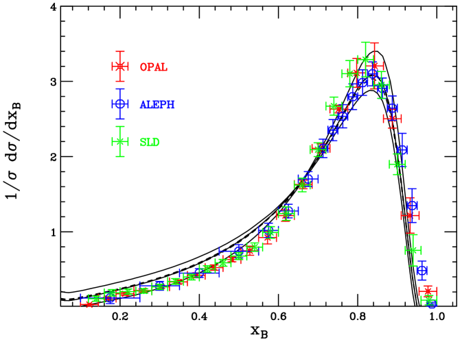
Figure 1: $B$-hadron spectrum yielded by our resummed calculation using the analytic time-like coupling constant $\tilde{\alpha}_{S}(k^{2})$ to model non-perturbative effects. We investigate the dependence on the factorization scales. Solid lines: $\mu_{0F}\,=\,m_{b}/2$, $m_{b}$ and $2m_{b}$; dashed lines: $\mu_{F}\,=\,m_{Z}/2$, $m_{Z}$ and $2m_{Z}$. The other parameters are kept to their default values.

Figure 2: Dependence on the renormalization scales $\mu_{R}$ and $\mu_{0R}$. Solid lines: $\mu_{R}$ varied between $m_{Z}/2$ and $2\,m_{Z}$; dashed lines: $\mu_{0R}$ between $m_{b}/2$ and $2\,m_{b}$.

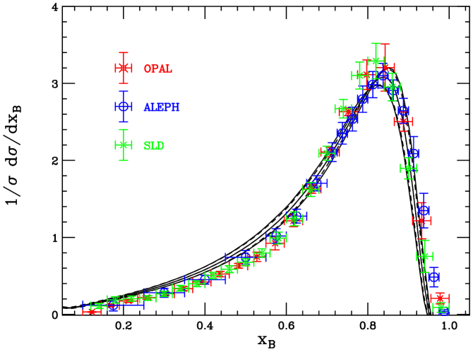
Figure 3: Dependence of the $B$-energy distribution on $\alpha_{S}(m_{Z}^{2})$ and on $m_{b}$. Solid lines: standard coupling $\alpha_{S}(m_{Z}^{2})$ varied from $0.117$ to $0.121$; Dashed lines: $b$ pole mass varied from $4.7$ to $5.3$ GeV.

.

In Fig. 1 we show the data points and our prediction, investigating its dependence on the factorization scales $\mu_{F}$ and $\mu_{0F}$. In Fig. 2 we look instead at the dependence on the renormalization scales $\mu_{R}$ and $\mu_{0R}$. For $\mu_{R}$ and $\mu_{F}$ we choose the values $m_{Z}/2$, $m_{Z}$ and $2m_{Z}$; for $\mu_{0R}$ and $\mu_{0F}$, $m_{b}/2$, $m_{b}$ and $2m_{b}$. We vary each scale separately, keeping all other quantities to their default values, in order to avoid an excessive number of runs. In Fig. 1 we notice that the dependence of our prediction on $\mu_{0F}$, the factorization scale entering in the initial condition of the perturbative fragmentation function, is rather large, especially at small $x_{B}$ and around the peak. At small $x_{B}$, the spectrum varies up to a factor of 2 if $\mu_{0F}$ changes from $m_{b}/2$ to $2m_{b}$; around the peak the impact of the choice of $\mu_{0F}$ is about 20%. The effect of the value chosen for $\mu_{F}$ is instead pretty small, and well within the band associated with the variation of $\mu_{0F}$. A possible explanation of the fairly large dependence on $\mu_{0F}$ could be the fact that, although we are working in the NNLL approximation, we are still matching the resummation to the NLO exact result, and not to the NNLO one. This generates a mismatch between the NNLL terms in the resummed expressions ($\sim\alpha_{S}^{2}\ln N$, $\alpha_{S}^{3}\ln^{2}N,\dots$) and the remainder functions, given in Eqs. (4.30) and (5.20), which have been included only to NLO. This mismatch is more evident in the initial condition, where $\mu_{0F}$ plays a role, since the coupling constant is larger, being evaluated at scales that are smaller than in the coefficient function. We should expect a milder dependence on such a factorization scale if we matched the resummed initial condition to the exact NNLO result [27]. Moreover, the scale $\mu_{0F}$ also enters in the DGLAP evolution operator (3.6), which we have implemented to NLL accuracy, using NLO splitting functions. Ref. [26] has recently calculated the NNLO corrections to the time-like splitting functions, which include a contribution analogous to the one $\sim A^{(3)}$ entering in the resummed expressions (4.5) and (5.4). The fact that we have not included such effects may be a further source of mismatch, which may be fixed implementing the splitting functions to NNLO accuracy. In any case, a peculiar feature of our model is that, since we are not using any hadronization model, our theoretical error includes, at the same time, uncertainties of both perturbative and non-perturbative nature. The partonic calculations in Refs. [14, 16, 17], which are NLL/NLO and use the standard coupling constant, yield indeed a very mild dependence on the quantities which enter in the perturbative calculation. However, in order to predict hadron-level observables, these perturbative computations need to be convoluted with a non-perturbative fragmentation function, whose parameters, after being fitted to SLD and LEP data, exhibit errors which are typically of the order of $10\%$, in such a way that the hadron spectra still present fairly large uncertainties.

Turning back to Fig. 1, let us observe that our distributions become negative and oscillate at very small and at very large $x_{B}$. In fact, the coefficient function (2.7) presents a term of the form

$$\frac{\alpha_{S}(\mu_{R}^{2})\,C_{F}}{\pi}\,\ln x,$$ (8.5)

which is enhanced at small $x$ and has not been resummed in our analysis. In any case, that does not affect much the comparison with the data, since the latter are at $x>0.12$. The coefficient function (2.7) and the initial condition (3.4) also contain terms of the type

$$-\,\frac{\alpha_{S}(\mu_{R}^{2})\,C_{F}}{\pi}\,\ln(1-x)~{}~{}~{}~{}~{}~{}~{}{\rm and}~{}~{}~{}~{}~{}~{}~{}2\,\frac{\alpha_{S}(\mu_{0R}^{2})\,C_{F}}{\pi}\,\ln(1-x),$$ (8.6)

which become large for $x\to 1$ and have not been resummed. It is at present not known how to accomplish this task. The contributions in Eq. (8.6) are responsible of the oscillating behaviour at large $x_{B}$. It is conceivable that the inclusion of NNLO corrections to the coefficient function and the initial condition may partly stabilize the distribution at the endpoints. In any case, we are aware that our simple model, based on an extrapolation of the perturbative behaviour to small energy scales, is expected to fail for very large $x$. It is therefore safe discarding a few data points at large $x_{B}$ when comparing with the data and, e.g., limiting ourselves to $x_{B}\,\raisebox{-3.0pt}{$\>\stackrel{{\scriptstyle<}}{{\scriptstyle\sim}}\>$}\,0.92$. We find that our default parameters give a good description of the ALEPH data ($\chi^{2}/\mathrm{dof}\,=\,21.4/16$), but reproduce rather badly the OPAL ($\chi^{2}/\mathrm{dof}\,=\,162.7/18$) and SLD ($\chi^{2}/\mathrm{dof}\,=\,109.1/20$) ones. The overall $\chi^{2}/\mathrm{dof}$, computed as if all measurements were coming from one experiment is also quite large: $\chi^{2}/\mathrm{dof}\,=\,293.2/54$. A much better description of SLD, OPAL and the overall sample is obtained setting $\mu_{0F}\,=\,m_{b}/2$. We obtain: $\chi^{2}/\mathrm{dof}=$ 24.8/16 (ALEPH), 30.4/18 (OPAL), 47.8/20 (SLD) and 103.0/54 (overall). Such values of $\chi^{2}/\mathrm{dof}$ are perfectly acceptable, since we are comparing data from different experiments and, as already discussed, SLD and OPAL, unlike ALEPH, also reconstructed a small fraction of $b$-flavoured baryons.

The theoretical uncertainties due to the values chosen for $\alpha_{S}(m_{Z}^{2})$ and $m_{b}$ are explored in Fig. 3: we consider $\alpha_{S}(m_{Z}^{2})\,=$ 0.117, 0.119 and 0.121 , and $m_{b}\,=\,4.7$, $5.0$ and $5.3$ GeV. The impact of the choice of these quantities is comparable and well visible throughout all the $x_{B}$-range, though smaller than the one due to the variation of $\mu_{0F}$. The effect is about 10% at average values of $x_{B}$ and grows up to 35% at large $x$. While changing $\alpha_{S}(m_{Z}^{2})$ and $m_{b}$ does not improve much the comparison with OPAL and SLD, an excellent description of the ALEPH data ($\chi^{2}/\mathrm{dof}=11.9/16$) is obtained for $m_{b}\,=\,5.3$ GeV, a value compatible with $B$-meson masses, and still $\alpha_{S}(m_{Z}^{2})=0.119$. Nevertheless, the comparison with the other experiments gets worse for this value of the bottom-quark mass, as we get $\chi^{2}/\mathrm{dof}=116.1/18$ for OPAL, 84.2/20 for SLD and 212.2/54 overall. As for the $\overline{\mbox{MS}}$ masses $\bar{m}_{b}$, $\bar{m}_{c}$ and $\bar{m}_{s}$, the effect of their variation on the $x_{B}$-spectrum is very little: we do not show such plots for the sake of brevity. The most relevant values of $\chi^{2}/\mathrm{dof}$ when we vary the perturbative parameters are collected in Table 1.

Table 1: Results of the comparison of our model with LEP and SLD data, for the most significant values of $\mu_{0F}$ and $m_{b}$. We have set $\alpha_{S}(m_{Z}^{2})=0.119$, while the other parameters have very little impact.

$\mu_{0F}$	$m_{b}$	$\chi^{2}/\mathrm{dof}$ (ALEPH)	$\chi^{2}/\mathrm{dof}$ (OPAL)	$\chi^{2}/\mathrm{dof}$ (SLD)	$\chi^{2}/\mathrm{dof}$ (overall)
$m_{b}$	5 GeV	21.4/16	162.18/18	109.1/20	293.2/54
$m_{b}/2$	5 GeV	24.8/16	30.4/18	47.8/20	103.0/54
$m_{b}$	5.3 GeV	11.9/16	116.1/18	84.2/20	212.2/54

8.2 Relevance of NNLL effects

Before turning to the analysis in moment space, we wish to estimate the impact on our prediction of the NNLL threshold-resummation corrections.

In Fig. 4 we present the experimental points and the spectra yielded by our model using the parameters which give the overall best fit to the data ($\mu_{0F}\,=\,m_{b}/2$ and $m_{b}\,=\,5$ GeV), but within two approximations schemes: NNLL soft resummation along with NNLO effective coupling constant (solid line), and NLL soft resummation with NLO coupling constant (dashed). In the NLO/NLL prediction, we still perform the Mellin transforms of the resummed expressions exactly, i.e. without the step-function approximation (4.16). By dropping the NNLL terms, i.e. the contributions proportional to $\tilde{A}^{(3)}$, $B^{(2)}$ and $D^{(2)}$ in the resummed expressions (4.5) and (5.4), we see that the spectrum gets shifted to larger $x_{B}$, and the agreement with the experimental data gets worse . For $x_{B}\,\raisebox{-3.0pt}{$\>\stackrel{{\scriptstyle<}}{{\scriptstyle\sim}}\>$}\,0.92$ we obtain: $\chi^{2}/\mathrm{dof}\,=\,11.18$ (SLD), $7.01$ (ALEPH), $16.27$ (OPAL) and $12.05$ (overall). The inclusion of the NNLL threshold contributions to the coefficient function and to the initial condition of the perturbative fragmentation function, together with the NNLO corrections to $\tilde{\alpha}_{S}(k^{2})$, is therefore crucial to get reasonable agreement with the data and the $\chi^{2}/\mathrm{dof}$ quoted in Table 1. In fact, when using the time-like coupling constant, the ${\cal O}(\alpha_{S}^{3})$ coefficient $A^{(3)}$ in the NNLL-resummed coefficient function and in the initial condition gets enhanced according to Eq. (7.6). The change $A^{(3)}\to\tilde{A}^{(3)}$ shifts the peak of the spectrum towards a lower value of $x_{B}$. If we had used the space-like coupling constant $\bar{\alpha}_{S}(k^{2})$, given in Eq. (6.3), instead of $\tilde{\alpha}_{S}(k^{2})$, we would have obtained the same $A^{(3)}$ and a rather poor description of the data.

It is also interesting to gauge the overall impact of the inclusion of power corrections by means of our model. In Fig. 4 we also show the NLL-resummed parton-level spectrum of Ref. [14], where the standard NLO coupling constant is used, the Mellin transforms are performed by the step-function approximation, and the inversion to $x$-space is done using the minimal prescription [36] to avoid the Landau pole. We see that the distribution of Ref. [14] is peaked at very large $x$ and is very far from the data for $x_{B}\,>\,0.4$. In fact, the $b$-quark spectrum of [14] is expected to be convoluted with a non-perturbative fragmentation function, whose parameters need to be fitted to reproduce the data. Our spectrum is also broader than the one of [14]: one can actually show that this is due to the fact that we have performed the Mellin transforms exactly.

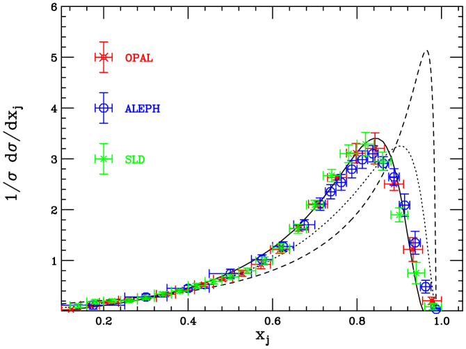
Figure 4: The solid line is our best prediction for $B$-hadron production ($j\,=\,B$), obtained using NNLL threshold resummation and the NNLO time-like coupling, super-imposed to the data. The dotted curve is obtained by dropping the NNLL terms, i.e. working within NLL accuracy. The dashed line is the parton-level spectrum of Ref. [14] ($j=b$), which uses the standard $\alpha_{S}(k^{2})$ and NLL large-$x$ resummation.

9 Phenomenology — $N$-space

We would like to present the results yielded by our approach in Mellin moment space, and compare them with the measurements of the DELPHI experiment [4]. It was argued in [19] that working in $N$-space is theoretically preferable, since one does not need to assume any functional form for the non-perturbative fragmentation function and can fit directly its moments. Moreover, as shown in [18, 7], the moments obtained fitting a non-perturbative model discarding data points at small and large $x_{B}$ are quite uncorrect, since the tails of the distributions play a crucial role to obtain the right $N$-space results. Our case is clearly different, since we are not tuning a non-perturbative fragmentation function, and therefore we do not have the problems related to the fits. However, our distributions are still negative and unreliable at very small and large $x_{B}$, and we were forced to discard few data points to obtain acceptable values of $\chi^{2}/\mathrm{dof}$. It is therefore still interesting to present the moments obtained using the analytic coupling constant and explore the theoretical uncertainties, by changing the parameters which enter in the calculation, along the lines of our $x$-space analysis. We calculate the $B$ spectrum in Mellin space directly from Eq. (8.2), and choose the same default values for scales, quark masses and $\alpha_{S}(m_{Z}^{2})$ as in $x$-space.

Table 2: Moments $\sigma^{B}_{N}$ from DELPHI [4] and moments $[\sigma_{N}^{B}]_{\mathrm{th}}$ yielded by our calculation. We quote the uncertainties due to the parameters which enter in the perturbative calculations, varied as discussed in the text. The theoretical total error is estimated as the sum in quadrature of the partial errors. We also present the moments $\sigma_{N}^{b}$ according to Ref. [14].

	$\langle x\rangle$	$\langle x^{2}\rangle$	$\langle x^{3}\rangle$	$\langle x^{4}\rangle$
$e^{+}e^{-}$ data $\sigma_{N}^{B}$	${\bf 0.7153\pm 0.0052}$	${\bf 0.5401\pm 0.0064}$	${\bf 0.4236\pm 0.0065}$	${\bf 0.3406\pm 0.0064}$
$[\sigma_{N}^{B}]_{\mathrm{th}}$	${\bf 0.6867\pm 0.0403}$	${\bf 0.5019\pm 0.0472}$	${\bf\,0.3815\pm 0.0465}$	${\bf\,0.2976\pm 0.0462}$
$\delta\sigma_{N}^{B}(\mu_{R})$	0.0014	0.0011	0.0009	0.0007
$\delta\sigma_{N}^{B}(\mu_{F})$	0.0066	0.0067	0.0059	0.0051
$\delta\sigma_{N}^{B}(\mu_{0R})$	0.0022	0.0028	0.0031	0.0033
$\delta\sigma_{N}^{B}(\mu_{0F})$	0.0364	0.0414	0.0398	0.0364
$\delta\sigma_{N}^{B}(m_{b})$	0.0111	0.0145	0.0153	0.0150
$\delta\sigma_{N}^{B}(\bar{m}_{b})$	0.0004	0.0005	0.0006	0.0006
$\delta\sigma_{N}^{B}(\bar{m}_{c})$	0.0003	0.0005	0.0006	0.0006
$\delta\sigma_{N}^{B}(\bar{m}_{s})$	0.0004	0.0007	0.0008	0.0008
$\delta\sigma_{N}^{B}(\alpha_{S}(m_{Z}^{2}))$	0.0113	0.0158	0.0173	0.0176
$\sigma_{N}^{b}$	0.7734 $\pm$ 0.0232	0.6333 $\pm$ 0.0311	0.5354 $\pm$ 0.0345	0.4617 $\pm$ 0.0346

In Table 2 we present the results of our study: we quote the experimental moments measured by DELPHI, the central values yielded by our calculation, denoted by $(\sigma_{N}^{B})_{\mathrm{th}}$, and the errors due to all the quantities which we vary. The data correspond to $N=$ 2, 3, 4 and 5; the first moment is $\sigma_{N=1}^{B}=1$, since both data and our spectra are normalized to unity. We estimate the overall theoretical error summing in quadrature the errors due to the variation of each parameter.

We observe that the experimental moments exhibit very little errors and that our central values are smaller by about $5\div 10\%$ than the DELPHI ones. This result confirms what we had found in $x_{B}$-space: our $x_{B}$-spectra go to zero more rapidly than the experimental data for large $x_{B}$, and become negative for $x_{B}>0.96$; for low and intermediate $x_{B}$, our curves lie above the data. It is therefore reasonable that our moments are smaller than the measured ones. However, we find that, within the uncertainties due to masses and scales, our calculation is in fair agreement with the data. As observed for the $x_{B}$-spectrum, the uncertainty due to the choice of $\mu_{0F}$ is pretty large, and the ones due to $\alpha_{S}(m_{Z}^{2})$ and $m_{b}$ are smaller but visible. The other scales and the $\overline{\mbox{MS}}$ masses, entering in the matching of $\alpha_{S}$ at different flavour numbers, have very little impact on the moments of the $B$ cross section. As far as the uncertainties are concerned, we observe that the DELPHI data are for $N\,\leq\,5$, hence the terms $\sim\ln^{k}N$ in the resummed exponents are not so dominant with respect to other contributions, such as the constants. Therefore, even in $N$-space, we expect that the further inclusion of NNLO contributions will have a significant impact on the prediction and decrease the theoretical error.

We also present in Table 2 the moments yielded by the NLL-resummed calculation of [14], which uses the NLO standard $\alpha_{S}(k^{2})$, whose $x$-space results have already been displayed in Fig. 4. We estimate the error on the moments of Ref. [14] as we did for the one on our calculation, varying the perturbative parameters in the same range. We find that the $N$-space results of [14], denoted by $\sigma_{N}^{b}$ to stress that they are a parton-level result, are very far from the data and much larger than the moments obtained using the analytic coupling constant. This result is in agreement with the plots in Fig. 4, and confirms the remarkable impact of non-perturbative effects in $N$-space as well. Moreover, we observe that the errors on the moments of [14] are smaller than the ones yielded by our calculation. In fact, Ref. [14] employs NLL threshold resummation and DGLAP evolution, and matches the resummation to the NLO results. As already discussed in the $x$-space analysis, using NNLL large-$x$ resummation but still NLL DGLAP evolution and NLO remainder functions, as we did, may lead to a mismatch which produces larger uncertainties. We expect that the inclusion of NNLO corrections to the initial condition and to the splitting functions will lead to a weaker dependence on the input parameters of our analysis. In any case, the perturbative moments of [14] need to be multiplied by the moments of a non-perturbative fragmentation function extracted from the data, which will lead to larger uncertainties on the hadron-level moments.

10 Conclusions

We studied $B$-hadron energy distributions in $e^{+}e^{-}$ annihilation at the $Z^{0}$ peak by means of a model having as the source of non-perturbative corrections an effective QCD coupling constant.

The physical idea behind our model is that the main non-perturbative effects, related to soft interactions in hadron bound states, are not very strong coupling phenomena, but can be described by an effective coupling constant of intermediate strength, typically $\tilde{\alpha}_{S}\,\approx\,0.3-0.5$. That implies that, within our model, these non-perturbative corrections — the Fermi motion in $B$ decays being the best-known example — can be obtained from perturbation theory by means of an extrapolation.

We modelled power corrections using a NNLO effective $\tilde{\alpha}_{S}(k^{2})$ constructed removing first the Landau pole, according to an analyticity requirement, and then resumming to all orders the absorptive effects related to time-like gluon branching. The resulting $\tilde{\alpha}_{S}(k^{2})$ significantly differs from the standard $\alpha_{S}(k^{2})$ at small scales. We described $b$-quark production within the framework of perturbative fragmentation functions, resumming threshold logarithms in the coefficient function and in the initial condition of the perturbative fragmentation function to NNLL accuracy, and matching the resummed results to the NLO ones. The perturbative fragmentation function was evolved using NLL DGLAP equations. When implementing threshold resummation in $N$-space, as part of our model, we decided to perform the Mellin transforms exactly, which leads to the further inclusion in the Sudakov exponent of terms $\sim\ln^{k}N$ of higher order (N³LL, N⁴LL, $\dots$), along with some constants and power-suppressed terms ${\cal O}\left(1/N\right)$.

We presented results on the $B$-hadron energy distribution, relying on this model to include power corrections, without introducing any non-perturbative fragmentation function with tunable parameters. When studying the $B$ spectra, we investigated the dependence of our prediction on the quantities which enter in the perturbative calculation, such as quark masses, renormalization and factorization scales, and $\alpha_{S}(m_{Z}^{2})$. We observed that the $x_{B}$-distributions become negative and oscillating at very small and large $x_{B}$, which is due terms $\sim\ln x$ and $\sim\ln(1-x)$, that are present in the NLO remainder functions and have not been resummed. We have therefore discarded a few data points at large $x_{B}$, where our calculation is anyway unreliable, and limited ourselves to $x_{B}\raisebox{-3.0pt}{$\>\stackrel{{\scriptstyle<}}{{\scriptstyle\sim}}\>$}0.92$. We compared our results with OPAL, ALEPH and SLD data on $b$-flavoured hadron production and found that, within our theoretical uncertainties, our calculation is able to reproduce quite well the ALEPH and OPAL data, while it is marginally consistent with SLD. As for the dependence on the perturbative parameters, the effect of the choice of the factorization scale $\mu_{0F}$, appearing in the initial condition of the perturbative fragmentation function, is quite large and the data are better described for low values of $\mu_{0F}$. The dependence on $\alpha_{S}(m_{Z}^{2})$ and on $m_{b}$ is also quite visible: for example, a value of $m_{b}$ consistent with $B$-meson masses, which is reasonable since our model assumes $E_{B}\,\simeq\,E_{b}$, yields an excellent description of the ALEPH data. The other parameters have instead very little impact on the $x_{B}$-spectrum.

We also compared our results in Mellin space with the moments measured by the DELPHI collaboration. We found that the central values of our $N$-space results are smaller than the experimental ones, but nonetheless, within the theoretical uncertainties, our moments are consistent with the data. In particular, a fairly large uncertainty is still due to the choice of $\mu_{0F}$, as was observed in the $x$-space analysis.

In summary, we find it remarkable that, within our theoretical uncertainties, we have been able to describe the LEP data in both $x$- and $N$-spaces, by modelling non-perturbative corrections via the analytic time-like coupling constant and without tuning any parameter to such data. It is also pretty interesting that a model which succeeded in reproducing the photon- and hadron-mass energy distribution in $B$-meson decays [9] has led to a reasonable fit of $B$-production data, although they are quite different processes, characterized by different energy scales.

Our model looks therefore quite promising and we plan to further apply it to other processes and observables. A straightforward extension of the study here presented is the investigation of $B$ production in top and Higgs decays, using the perturbative calculations in [16, 15, 17], and modelling power corrections as in the present paper. We can also use our model along with Monte Carlo event generators: in Ref. [18], the hadronization models of HERWIG and PYTHIA were tuned to the same data as the ones here considered, and then used to predict $B$ production in top and Higgs decays. We may thus think of using the parton shower algorithms of HERWIG and PYTHIA to describe perturbative $b$-production, with our analytic coupling constant in place of the cluster and string models. At the end of the cascade, we can assume $E_{b}\to E_{B}$ and compare the results with the data. The spectra yielded by Monte Carlo event generators are positive definite and do not exhibit the problem of becoming negative. However, parton shower algorithms are equivalent to a LL/LO resummation, with the further inclusion of some NLLs [49]. Since we have learned from this analysis that the inclusion of corrections of higher orders is crucial to reproduce the data, we may have to add to the Monte Carlo Sudakov form factor contributions analogous to the NLLs and NNLLs that are missing, in particular the one $\sim\tilde{A}^{(3)}$.

Besides, it will be really worthwhile to use the recent calculations of the NNLO initial condition of the perturbative fragmentation function [27, 28] and of the NNLO splitting functions in the non-singlet sector [29] to fully promote our formalism to NNLO/NNLL accuracy. This way we could explore whether the uncertainties on our predictions — especially the one due to the scale $\mu_{0F}$ — get finally reduced. If the theoretical uncertainties get substantially reduced, one may even think of extracting $\alpha_{S}(m_{Z}^{2})$ from $b$-fragmentation data, as already done from $B$-decay spectra [9].

Our study could also be improved by including NNNLL contributions in the resummation exponents. Such corrections involve the coefficients $A^{(4)}$, $B^{(3)}$ and $D^{(3)}$: at present only $B^{(3)}$ is exactly known. In particular, we expect a relevant effect due to the possible inclusion of $D^{(3)}$, the ${\cal O}(\alpha_{S}^{3})$ coefficient of function $D(\alpha_{S})$, which resums large-angle soft radiation in the initial condition. In fact, we have observed that the scale of $\alpha_{S}$ in the resummed initial condition is smaller than in the coefficient function, and therefore power corrections are more relevant. Also, our model enhances the coefficients of $\alpha_{S}$ from the third order on. We can therefore employ our model to implement non-perturbative corrections to Drell–Yan or Deep Inelastic Scattering processes, whose coefficient function was recently calculated to NNNLO accuracy [50]. In $e^{+}e^{-}$ annihilation, threshold contributions to the NNNLO coefficient function were computed in [51]; the full ${\cal O}(\alpha_{S}^{3})$ corrections have not been calculated yet.

From the theoretical viewpoint, we plan to investigate in more detail the issue of the Mellin transform of the resummed cross section and the power corrections which are inherited by the $B$ spectrum when one uses the effective $\tilde{\alpha}_{S}(k^{2})$ and does the longitudinal-momentum integration in an exact or approximated way. Within our model, we chose to perform it exactly, driven by the results in [9, 44], but nonetheless we believe that a thorough study of this point, along the lines of [36, 35], should be necessary.

Other issues which we plan to investigate in detail are the treatment of the higher orders of the effective $\tilde{\alpha}_{S}$ and the comparison between time- and space-like coupling constants. We have obtained reasonable agreement with the data by using the time-like effective coupling constant and taking the powers $\tilde{\alpha}_{S}^{n}(k^{2})$ after performing the integral of the dispersion relation. Nonetheless, this conclusion is somehow related to the level of approximation of the perturbative calculation which we have employed, and may not hold if we used a different accuracy. Therefore, a more solid understanding of these aspects of our model is mandatory.

Furthermore, our model has some built-in universal features implying that, to put it into a stringent check, one should consider several observables from different processes. To this goal, however, one might need both NNLL resummation from the theoretical side and accurate data on the experimental one. Shape-variable data at the $Z^{0}$ peak, for example, are rather accurate, but for these quantities NNLL resummation is still in progress, hence preventing an analysis within our model. In [9] this model was applied to semi-inclusive $B$ decays, where the situation is somehow complementary with respect to shape variables in $e^{+}e^{-}$ annihilation: NNLL threshold resummation is well established, but data are not very accurate yet, because of large backgrounds.

Finally, we could also push our model to the ‘low-energy’ direction, to try to describe, for example, charm production at the $Z^{0}$ peak or below it, where accurate experimental data are available. Due to the large value of $\alpha_{S}(m_{c}^{2})\simeq 0.35$ and to a soft scale $S\simeq m_{c}(1-x)$, smaller by a factor of three than in $b$-production, we expect a full NNLL/NNLO analysis to be necessary. The comparison with $D$-hadron data will be crucial to investigate possible deviations from our model. In fact, an extension of the formulation here presented may consist in adding to $\tilde{\alpha}_{S}(k^{2})$ a correcting term: $\tilde{\alpha}^{\prime}_{S}(k^{2})=\tilde{\alpha}_{S}(k^{2})+\delta\tilde{\alpha}_{S}(k^{2})$. This way, $\tilde{\alpha}_{S}(k^{2})$ will still be the effective coupling constant here discussed, while $\delta\tilde{\alpha}_{S}(k^{2})$ will depend on the hadronic state which we wish to describe, and vary, e.g, from mesons to baryons or from $B$’s to $D$’s. Investigating the charm sector may therefore help in shedding light on our model and understanding whether such a correcting term is necessary or not. This study is in progress as well.

Acknowledgments

We are indebted to S. Catani for discussions on soft-gluon resummation. We also acknowledge M. Cacciari for discussions on the perturbative fragmentation approach and for providing us with the computing code to obtain the results of Ref. [14].

Appendix A Numerical evaluation of Mellin transforms

In this appendix we present a method for computing numerically the Mellin transform, through the Fast Fourier Transform (FFT), of a function of the form

$$f(y)\,=\,\left[\frac{\varphi(y)}{y}\right]_{+},$$ (A.1)

where $y\,=\,1-z$ and $\varphi(y)$ is a regular function of $y$ or a function having at most a logarithmic singularity for $y\,\to\,0$.

To calculate the integer moments of the cross section $\sigma_{N}$ — typically the first few moments with $N=2,3,4,5,\cdots$ — the integral defining the Mellin transform does not present any convergence problem and can be done directly. In order to obtain the cross section in $x$-space, it is however necessary to perform an inverse Mellin transform by integrating $\sigma_{N}$ along a vertical line in $N$-space. The numerical computation of $\sigma_{N}$ in the complex $N$-plane is non trivial for ${\rm Im}\,N\,\gg\,1$ because the kernel $z^{N-1}$ develops fast oscillations with $z$, which affect the convergence of the integral.

In detail, we have to compute the integral

$$g_{N}\,=\,\int_{0}^{1}dy(1-y)^{N-1}\,f(y)\,=\,\int_{0}^{1}\frac{dy}{y}\,\left[(1-y)^{N-1}-1\right]\,\varphi(y).$$ (A.2)

for $N$ lying on a vertical line in the complex plane,

$$N\,=\,c\,+\,i\nu,$$ (A.3)

with $c\,>\,0$ and $\nu$ real. It is convenient to treat analytically the infrared cancellation between real and virtual contributions related to the first and the second term in square brackets on the r.h.s. of Eq. (A.2). We then take a derivative with respect to $\nu$:

$$\gamma_{c}\left(\nu\right)\,\equiv\,\frac{dg_{c+i\nu}}{d\nu}\,=\,i\int_{0}^{1}dy\,\frac{\ln(1-y)}{y}\,(1-y)^{c-1+i\nu}\,\varphi(y).$$ (A.4)

Note that the infrared singularity $1/y$ is now regulated by the $\ln(1-y)$ factor coming from the differentiation.

In order to express $\gamma_{c}(\nu)$ as the Fourier transform (FT) of some function, we change variables to

$$t\,\equiv\,-\,\ln(1-y),$$ (A.5)

and express Eq. (A.4) as an integral over $t$:

$$\gamma_{c}\left(\nu\right)\,=\,\int_{0}^{\infty}dt\,e^{-\,i\,\nu\,t}\,\psi_{c}(t),$$ (A.6)

with

$$\psi_{c}(t)\,\equiv\,-i\,\frac{t}{1\,-\,e^{-t}}\,e^{-c\,t}\,\varphi\left[1\,-\,e^{-t}\right].$$ (A.7)

$\gamma_{c}$ is therefore the Fourier transform of the function $\psi_{c}(t)$ defined above and vanishing for $t\,<\,0$. For a fast numerical evaluation, it is convenient to transform the FT above into a Fast-Fourier-Transform (FFT). We cut the improper integral at a large but finite $t_{\max}$:

$$\gamma_{c}\left(\nu\right)\,\simeq\,\int_{0}^{t_{\max}}dt\,e^{-\,i\,\nu\,t}\,\psi_{c}(t).$$ (A.8)

In practice, because of the exponential dependence $y\,\approx\,\exp[-t]$, we found that $t_{\max}\,=\,20\div 30$ already gives a good accuracy. The above integral can be easily approximated by means of a constant sampling:

$$\Delta t\,\equiv\,\frac{t_{\max}}{n},$$ (A.9)

where $n$ is the number of points in which the function $\psi_{c}(t)$ is evaluated. We have found that an accuracy $O(10^{-3}\div 10^{-4})$ is reached already with $n\,=\,10^{4}\div 10^{5}$ points. We then have:

$$\gamma_{c}\left(\nu\right)\,\cong\,\,e^{-\,i/2\,\nu\,\Delta t}\,\Delta t\,\sum_{k=0}^{n-1}e^{-i\,\nu\,k\,\Delta t}\,\psi_{c}\left[\left(k+\frac{1}{2}\right)\Delta t\right].$$ (A.10)

The Mellin transform is obtained by a numerical integration of $\gamma_{c}(\nu)$:

$$g_{c+i\nu}\,=\,g_{c}\,+\,\int_{0}^{\nu}d\nu^{\prime}\,\gamma_{c}\left(\nu^{\prime}\right).$$ (A.11)

$g_{c}$ is the Mellin transform in the fixed point $c$ on the positive $N$ axis; it is a constant which is computed directly just once. Eq. (A.11) is our final result for the numerical computation of the Mellin transform.

Let us now discuss the numerical computation of the inverse Mellin transform with a similar method:

$$f(y)\,=\,\int_{c-i\infty}^{c+i\infty}\frac{dN}{2\pi i}\,(1-y)^{-N}\,g_{N}\,=\,\frac{1}{(1-y)^{c}}\,\int_{-\infty}^{+\infty}\frac{d\nu}{2\pi}\,(1-y)^{-i\nu}\,g_{c+i\nu}.$$ (A.12)

Since $f(y)$ is real, one immediately obtains the following property of its Mellin transform:

$$\left(g_{N}\right)^{*}\,=\,g_{N^{*}}.$$ (A.13)

The inverse Mellin transform can therefore also be written as:

$$f(y)\,=\,\frac{1}{\pi\,(1-y)^{c}}\,{\mathrm{Re}}\,\int_{0}^{\infty}d\nu\,e^{-\,i\,\nu\,\ln(1-y)}\,g_{c\,+\,i\,\nu}.$$ (A.14)

Apart from constant factors, Eq. (A.14) express the inverse Mellin transform as the inverse Fourier transform $\nu\,\to\,-\,\ln(1-y)$ of $g_{c+i\nu}$. The transformation to the Inverse Fast Fourier Transform can be made as in the direct case.

We have implemented the above algorithm within the Mathematica System with a gain of CPU time by over an order of magnitude with respect to the direct numerical evaluation. A typical run on a standard PC takes ${\cal O}(1)$ minute. We have also checked our numerical results with direct integration in Fortran.

References

• [1] SLD Collaboration, K. Abe et al., Phys. Rev. Lett. 84 (2000) 4300.
• [2] ALEPH Collaboration, A. Heister et al., Phys. Lett. B512 (2001) 30.
• [3] OPAL Collaboration, G. Abbiendi et al., Eur. Phys. J. C29 (2003) 463.
• [4] DELPHI Collaboration, G. Barker et al., DELPHI 2002-069, CONF 603.
• [5] V.G. Kartvelishvili, A.K. Likehoded and V.A. Petrov, Phys. Lett. B78 (1978) 615.
• [6] C. Peterson, D. Schlatter, I. Schmitt and P.M. Zerwas, Phys. Rev. D27 (1983) 105.
• [7] M. Cacciari and E. Gardi, Nucl. Phys. B664 (2003) 299.
• [8] E. Gardi, Nucl. Phys. B622 (2002) 365.
• [9] U. Aglietti, G. Ferrera and G. Ricciardi, Nucl. Phys. B768 (2007) 85.
• [10] See, for example:
Yu. L. Dokshitzer, V.A. Khoze, A.H. Mueller and S.I. Troian, Basics of Perturbative QCD, Gif-sur-Yvette, France: Editions Frontières, (1991) 274 p.;
R.K. Ellis, W.J. Stirling and B.R. Webber, QCD and Collider Physics, Camb. Monogr. Part. Phys. Nucl. Phys. Cosmol. 8 (1996) 1–435.
• [11] B. Mele and P. Nason, Nucl. Phys. B361 (1991) 626.
• [12] L.N. Lipatov, Sov. J. Nucl. Phys. 20 (1975) 95; V.N. Gribov and L.N. Lipatov, Sov. J. Nucl. Phys. 15 (1972) 438; Yu.L. Dokshitzer, Sov. Phys. JETP 46 (1977) 641.
• [13] G. Altarelli and G. Parisi, Nucl. Phys. B126 (1977) 298.
• [14] M. Cacciari and S. Catani, Nucl. Phys. B617 (2001) 253.
• [15] G. Corcella and A.D. Mitov, Nucl. Phys. B623 (2002) 247.
• [16] M. Cacciari, G. Corcella and A.D. Mitov, JHEP 0212 (2002) 015.
• [17] G. Corcella, Nucl. Phys. B 705 (2005) 363;
G. Corcella, Nucl. Phys. B 715 (2005) 609, Erratum.
• [18] G. Corcella and V. Drollinger, Nucl. Phys. B730 (2005) 82.
• [19] M. Cacciari and P. Nason, Phys. Rev. Lett. 89 (2002) 122003.
• [20] B. Ermolaev, M. Greco and S. Troyan, Phys. Lett. B522 (2001) 57.
• [21] D. Shirkov, Nucl. Phys. Proc. Suppl. 152 (2006) 51.
• [22] N. G. Stefanis, W. Schroers and H. C. Kim, Phys. Lett. B449 (1999) 299;
N. G. Stefanis, W. Schroers and H. C. Kim, Eur. Phys. J. C18 (2000) 137.
• [23] U. Aglietti and G. Ricciardi, Phys. Rev. D70 (2004) 114008.
• [24] G. Altarelli, R.K. Ellis, G. Martinelli and S.–Y. Pi, Nucl. Phys. B160 (1979) 301.
• [25] P.J. Rijken and W.L. van Neerven, Nucl. Phys. B487 (1997) 233.
• [26] A.D. Mitov and S. Moch, Nucl. Phys. B751 (2006) 18.
• [27] K. Melnikov and A.D. Mitov, Phys. Rev. D70 (2004) 034027.
• [28] A.D. Mitov, Phys. Rev. D71 (2005) 054021
• [29] A.D. Mitov, S. Moch and A. Vogt, Phys. Lett. B638 (2006) 61.
• [30] G. Sterman, Nucl. Phys. B281 (1987) 310.
• [31] S. Catani and L. Trentadue, Nucl. Phys. B327 (1989) 323.
• [32] S. Moch, J.A.M. Vermaseren and A. Vogt, Nucl. Phys B688 (2004) 101.
• [33] S. Catani, D. de Florian, M. Grazzini and P. Nason, JHEP 07 (2003) 028.
• [34] G.P. Korchemsky and G. Sterman, Nucl. Phys. B 437 (1995) 415.
• [35] M. Beneke and V.M. Braun, Nucl. Phys. B454 (1995) 253.
• [36] S. Catani, M.L. Mangano, P. Nason and L. Trentadue, Nucl. Phys. B478 (1996) 273.
• [37] S. Moch, J.A.M. Vermaseren and A. Vogt, Nucl. Phys. B646 (2002) 181.
• [38] E. Gardi, JHEP 0502 (2005) 053.
• [39] U. Aglietti and G. Ricciardi, Phys. Rev. D66 (2002) 074003.
• [40] U. Aglietti, G. Ferrera and G. Ricciardi, Phys. Rev. D74 (2006) 034004.
• [41] G. Corcella and A.D. Mitov, Nucl. Phys. B 676 (2004) 346.
• [42] D. Amati, A. Bassetto, M. Ciafaloni, G. Marchesini and G. Veneziano, Nucl. Phys. B173 (1980) 429.
• [43] W. Bernreuther, Ann. Phys. 151 (1983) 127;
W. Bernreuther and W. Wetzel, Nucl. Phys B197 (1982) 228;
W. Bernreuther and W. Wetzel, Nucl. Phys. B513 (1998) 758, Erratum.
• [44] U. Aglietti and G. Ricciardi, Phys. Rev. D70 (2004) 114008.
• [45] G. Corcella, I.G. Knowles, G. Marchesini, S. Moretti, K. Odagiri, P. Richardson, M.H. Seymour, B.R. Webber, JHEP 0101 (2001) 010.
• [46] T. Sjostrand, S. Mrenna and P. Skands, JHEP 0605 (2006) 026.
• [47] S. Eidelman et al., Phys. Lett. B592 (2004) 1.
• [48] U. Aglietti and G. Corbò, unpublished.
• [49] S. Catani, G. Marchesini and B.R. Webber, Nucl. Phys. B349 (1991) 635.
• [50] S. Moch, J.A.M. Vermaseren and A. Vogt, Nucl. Phys. B724 (2005) 3.
• [51] J. Blümlein and V. Ravindran, Phys. Lett. B640 (2006) 40.