Probe the R-parity Violating Supersymmetry Effects
in the $B^{0}_{s}-\bar{B}^{0}_{s}$ Mixing

Abstract

The recent measurements of the $B_{s}$ mass difference $\Delta M_{s}$ by the CDF and DØ collaborations are roughly consistent with the Standard Model predictions, therefore, these measurements will afford an opportunity to constrain new physics scenarios beyond the Standard Model. We consider the impact of the R-parity violating supersymmetry in the $B^{0}_{s}-\bar{B}^{0}_{s}$ mixing, and use the latest experimental results of $\Delta M_{s}$ to constrain the size of the R-parity violating tree level couplings in the $B^{0}_{s}-\bar{B}^{0}_{s}$ mixing. Then, using the constrained R-parity violating parameter space from $\Delta M_{s}$, we show the R-parity violating effects on the $B_{s}$ width difference $\Delta\Gamma_{s}$.

PACS Numbers: 12.60.Jv, 11.30.Er, 12.15.Mm, 14.40.Nd

Recently CDF and DØ collaborations have measured the mass difference in the $B^{0}_{s}-\bar{B}^{0}_{s}$ system [1, 2] with the results

CDF: $$\Delta M_{s}=(17.31^{+0.33}_{-0.18}\pm 0.07)/\mbox{ps},$$ (1)

DØ: $$17/\mbox{ps}<\Delta M_{s}<21/\mbox{ps}~{}~{}~{}~{}\mbox{(90\%~{}C.L.)}.$$ (2)

The measurement of CDF collaboration turned out to be surprisingly below the Standard Model (SM) predictions obtained from other constraints [3, 4]

$$\Delta M_{s}^{SM}(\mbox{UTfit})=(21.5\pm 2.6)/\mbox{ps},~{}~{}~{}\Delta M_{s}^{SM}(\mbox{CKMfit})=(21.7^{+5.9}_{-4.2})/\mbox{ps}.$$ (3)

A consistent though slightly smaller value is found for the mass difference directly from its SM expression in later Eq.(10)

$$\Delta M_{s}^{SM}(\mbox{Direct})=(20.8\pm 6.4)/\mbox{ps}.$$ (4)

with the input parameters collected in Table I. It’s noted that this prediction is sensitive to the value chosen for the non-perturbative quantity $F_{B_{s}}\sqrt{B_{B_{s}}}$ and the CKM matrix element $V_{ts}$, in this paper, we use their values from Refs.[3, 5]. The implication of $\Delta M_{s}$ measurements have already been studied in model independent approach [6], MSSM models [7], $Z^{\prime}$-model [8], Grand Unified Models [9].

The SM prediction in Eq.(4) suffers large uncertainties from the hadronic parameters, nevertheless, the experimental data agree fairly well with the SM value. Therefore, we can use the CDF measurement to constrain new physics which may induce the b-s transition. Effects of the R-parity violating (RPV) supersymmetry (SUSY) on the neutral meson mixing have been discussed extensively in the papers [10, 11]. In this paper we will consider the RPV SUSY effects at the tree level in the $B^{0}_{s}-\bar{B}^{0}_{s}$ mixing by the latest experimental data. Using the latest experimental data of $\Delta M_{s}$ and the theoretical parameters, we obtain the new bound on the relevant RPV coupling product. If there are RPV contributions to $\Delta M_{s}$, the same new physics will also contribute to the width difference $\Delta\Gamma_{s}$, and therefore we will use the constrained parameter region to examine the RPV effects on $\Delta\Gamma_{s}$.

We first consider the SM contribution to the $B^{0}_{s}-\bar{B}^{0}_{s}$ mixing. The SM effective Hamiltonian for the $B^{0}_{s}-\bar{B}^{0}_{s}$ mixing is usually described by [12]

$$\mathcal{H}_{eff}^{SM}=\frac{G_{F}^{2}}{16\pi^{2}}m_{W}^{2}|V_{ts}^{*}V_{tb}|^{2}\eta_{2B}S_{0}(x_{t})[\alpha_{s}(\mu_{b})]^{-6/23}\left[1+\frac{\alpha_{s}(\mu_{b})}{4\pi}J_{5}\right]\mathcal{O}+h.c.,$$ (5)

with

$$\mathcal{O}=(\bar{s}b)_{V-A}(\bar{s}b)_{V-A},$$ (6)

where $x_{t}=m^{2}_{t}/m^{2}_{W}$ and $\eta_{2B}$ is the QCD correction.

In terms of Eq.(5), the mixing amplitude $M_{12}^{s}$ in the SM, dominated by the top quark loop, is

$$M_{12}^{s,SM}=\frac{\langle B^{0}_{s}|\mathcal{H}_{eff}^{SM}|\bar{B}^{0}_{s}\rangle}{2m_{B_{s}}}.$$ (7)

Defining the renormalization group invariant parameter $B_{B_{s}}$ by

$$B_{B_{s}}=B_{B_{s}}(\mu)[\alpha_{s}(\mu)]^{-6/23}\left[1+\frac{\alpha_{s}(\mu)}{4\pi}J_{5}\right],$$ (8)

$$\langle B^{0}_{s}|\mathcal{O}|\bar{B}^{0}_{s}\rangle\equiv\frac{8}{3}B_{B_{s}}(\mu)F^{2}_{B_{s}}m_{B_{s}}^{2},$$ (9)

then, we have the $B_{s}$ mass difference in the SM

$$\Delta M_{s}^{SM} = 2\left|M_{12}^{s,SM}\right|$$ (10)

$$= \frac{G_{F}^{2}}{6\pi^{2}}m_{W}^{2}m_{B_{s}}|V_{ts}^{*}V_{tb}|^{2}\eta_{2B}S_{0}(x_{t})\left(F_{B_{s}}\sqrt{B_{B_{s}}}\right)^{2}.$$

In the SM, the off-diagonal element of the decay width matrix $\Gamma^{s,SM}_{12}$ may be written as [13]

$$\Gamma^{s,SM}_{12}=-\frac{G^{2}_{F}m^{2}_{b}}{24\pi M_{B_{s}}}\left|V_{cb}V_{cs}^{*}\right|^{2}\left[G(x_{c})\langle B^{0}_{s}|\mathcal{O}|\bar{B}^{0}_{s}\rangle+G_{2}(x_{c})\langle B^{0}_{s}|\mathcal{O}_{2}|\bar{B}^{0}_{s}\rangle+\sqrt{1-4x_{c}}\hat{\delta}_{1/m}\right],$$ (11)

here $x_{c}=m_{c}^{2}/m_{b}^{2}$, $G(x_{c})=0.030$ and $G_{2}(x_{c})=-0.937$ at the $m_{b}$ scale [13], and the $1/m_{b}$ corrections $\hat{\delta}_{1/m}$ are given in [14]. The operator $\mathcal{O}$ can be found in Eq.(6), one now encounters a second operator operator, $\mathcal{O}_{2}$, and thereby another B-parameter $B^{(s)}_{2}(\mu)$

$$\mathcal{O}_{2}=(\bar{s}b)_{S-P}(\bar{s}b)_{S-P},~{}~{}~{}\langle B^{0}_{s}|\mathcal{O}_{2}(\mu)|\bar{B}^{0}_{s}\rangle=-\frac{5}{3}\left(\frac{m_{B_{s}}}{\overline{m}_{b}(\mu)+\overline{m}_{s}(\mu)}\right)^{2}m^{2}_{B_{s}}f^{2}_{B_{s}}B^{(s)}_{2}(\mu).$$ (12)

The width difference between $B_{s}$ mass eigenstates is given by

$$\Delta\Gamma_{s}^{SM} = 2\left|\Gamma^{s,SM}_{12}\right|$$ (13)

$$= \frac{G^{2}_{F}m^{2}_{b}}{12\pi M_{B_{s}}}\left|V_{cb}V_{cs}^{*}\right|^{2}\left[\frac{8}{3}G(x_{c})B_{B_{s}}(\mu)F^{2}_{B_{s}}m_{B_{s}}^{2}\right.$$

$$\left.-\frac{5}{3}G_{2}(x_{c})\left(\frac{m_{B_{s}}}{\overline{m}_{b}(\mu)+\overline{m}_{s}(\mu)}\right)^{2}m^{2}_{B_{s}}f^{2}_{B_{s}}B^{(s)}_{2}(\mu)+\sqrt{1-4x_{c}}\hat{\delta}_{1/m}\right],$$

and the SM predicts $\Delta\Gamma_{s}^{SM}$ with the input parameters in Table I

$$\Delta\Gamma_{s}^{SM}(\mbox{Direct})=(0.07\pm 0.03)/\mbox{ps}.$$ (14)

It’s noted that the width difference have been reviewed recently in [15].

Now we turn to the RPV SUSY contributions to the $B^{0}_{s}-\bar{B}^{0}_{s}$ mixing. In the most general superpotential of the minimal supersymmetric Standard Model, the RPV superpotential is given by [16]

$$\mathcal{W}_{\not\!R_{p}\,} = \mu_{i}\hat{L}_{i}\hat{H}_{u}+\frac{1}{2}\lambda_{[ij]k}\hat{L}_{i}\hat{L}_{j}\hat{E}^{c}_{k}+\lambda^{\prime}_{ijk}\hat{L}_{i}\hat{Q}_{j}\hat{D}^{c}_{k}+\frac{1}{2}\lambda^{\prime\prime}_{i[jk]}\hat{U}^{c}_{i}\hat{D}^{c}_{j}\hat{D}^{c}_{k},$$ (15)

where $\hat{L}$ and $\hat{Q}$ are the SU(2)-doublet lepton and quark superfields, $\hat{E}^{c}$, $\hat{U}^{c}$ and $\hat{D}^{c}$ are the singlet superfields, while $i$, $j$ and $k$ are generation indices and $c$ denotes a charge conjugate field.

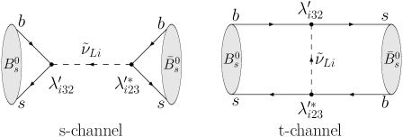
Figure 1: The RPV tree level contributions to the $B^{0}_{s}-\bar{B}^{0}_{s}$ mixing.

The $\lambda^{\prime}$ couplings of Eq.(15) make the $B^{0}_{s}-\bar{B}^{0}_{s}$ mixing possible at the tree level through the exchange of a sneutrino $\tilde{\nu}_{i}$ both in the s- and t-channels displayed in Fig.1. The RPV tree level contributions to $B^{0}_{s}-\bar{B}^{0}_{s}$ mixing are described by

$$\mathcal{H}^{\not\!R_{p}\,}_{eff}=\frac{1}{4}\sum_{i}\frac{\lambda^{\prime}_{i32}\lambda^{\prime*}_{i23}}{m^{2}_{\tilde{\nu}_{Li}}}(\bar{s}b)_{S-P}(\bar{s}b)_{S+P}+h.c.,$$ (16)

where we have a new physics operator

$$\mathcal{O}_{4}=(\bar{s}b)_{S-P}(\bar{s}b)_{S+P},$$ (17)

and we define the B-parameter as

$$\langle B^{0}_{s}|\hat{\mathcal{O}}_{4}(\mu)|\bar{B}^{0}_{s}\rangle = 2\left(\frac{m_{B_{s}}}{\overline{m}_{b}(\mu)+\overline{m}_{s}(\mu)}\right)^{2}m_{B_{s}}^{2}F_{B_{s}}^{2}B^{(s)}_{4}(\mu).$$ (18)

Note that the expectation values are scaled by factor of $2m_{B}$ over those given in some literature due to our different normalization of the meson wave functions. It is trivial to check that both conventions yield the same values for physical observables.

The RPV mixing amplitude $M_{12}^{s,\not\!R_{p}\,}$ is

$$M_{12}^{s,\not\!R_{p}\,} = \frac{\langle B^{0}_{s}|\mathcal{H}_{eff}^{\not\!R_{p}\,}|\bar{B}^{0}_{s}\rangle}{2m_{B_{s}}}$$ (19)

$$= \sum_{i}\frac{\lambda^{\prime}_{i32}\lambda^{\prime*}_{i23}}{m^{2}_{\tilde{\nu}_{Li}}}\frac{1}{4}\left(\frac{m_{B_{s}}}{m_{b}(\mu)+m_{s}(\mu)}\right)^{2}m_{B_{s}}F_{B_{s}}^{2}B^{(s)}_{4}(\mu),$$

Given the expressions above, we now write the total $B_{s}$ mass difference included both SM and RPV contributions

$$\Delta M_{s}=2|M^{s}_{12}|,$$ (20)

with

$$M^{s}_{12} = M^{s,SM}_{12}+M_{12}^{s,\not\!R_{p}\,}$$ (21)

$$= M^{s,SM}_{12}(1+ze^{i\theta}),$$

where the parameters $z$ and $\theta$ give the relative magnitude and relative phase of the RPV contribution, i.e. $z\equiv\left|M_{12}^{s\not\!R_{p}\,}/M^{s,SM}_{12}\right|$ and $\theta\equiv$arg$\left(M_{12}^{s,\not\!R_{p}\,}/M^{s,SM}_{12}\right)$.

The $B_{s}$ width difference beyond the SM has been studied in Refs.[17, 18]. If there are RPV contributions to $\Delta M_{s}$, the same new physics will also contribute to the $B_{s}$ width difference. The width difference including the RPV contributions is given by [18]

$$\Delta\Gamma_{s}=\frac{4|Re(M^{s}_{12}\Gamma^{s*}_{12})|}{\Delta M_{s}}=2|\Gamma^{s}_{12}|\cdot|\mbox{cos}\phi_{m}|,$$ (22)

where $\phi_{m}=$arg$(1+ze^{i\theta})$, and $\phi_{m}=0$ turns out to be an excellent approximation in the SM. The effect of NP on the off-diagonal element of the decay width matrix $\Gamma^{s}_{12}$ is anticipated to be negligibly small, hence $\Gamma^{s}_{12}=\Gamma^{s,SM}_{12}$ holds as a good approximation [19].

We now perform numerical calculation and show the constraint imposed by the measurement of $\Delta M_{s}$ only or both $\Delta M_{s}$ and $\Delta\Gamma_{s}$. The values of the input parameters used in this paper are collected in Table I, and we will use the input parameters and the experimental data which vary randomly within $1\sigma$ variance.

Table I: Values of the theoretical quantities as input parameters.

$m_{W}=80.403\pm 0.029~{}GeV,~{}~{}~{}m_{B_{s}}=5.3696\pm 0.0024~{}GeV,$
$\overline{m}_{b}(\overline{m}_{b})=4.20\pm 0.07~{}GeV,~{}~{}~{}\overline{m}_{s}(2GeV)=0.095\pm 0.025~{}GeV,$
$m_{t}=174.2\pm 3.3~{}GeV,~{}~{}~{}m_{b}=4.8~{}GeV$.	[20]
$A=0.818^{+0.007}_{-0.017},~{}~{}~{}\lambda=0.2272\pm 0.0010.$	[20]
$\eta_{2B}=0.55\pm 0.01.$	[21]
$F_{B_{s}}\sqrt{B_{B_{s}}}=0.262\pm 0.035~{}GeV,~{}~{}~{}F_{B_{s}}=0.230\pm 0.030~{}GeV.$	[5]
$B_{2}^{(s)}(m_{b})=0.832\pm 0.004,~{}~{}~{}B_{4}^{(s)}(m_{b})=1.172^{+0.005}_{-0.007}.$	[22]

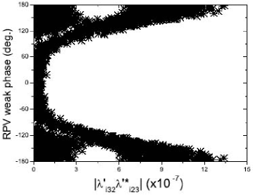
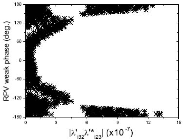
Figure 2: Allowed parameter space for $\lambda^{\prime}_{i32}\lambda^{\prime*}_{i23}$ constrained by the experimental data of $\Delta M_{s}$.

We calculate the contributions of Eq.(16) to $\Delta M_{s}$ and require it not to exceed the corresponding experimental data in Eq.(1). The random variation of the parameters subjecting to the constraint leads to the scatter plot shown in Fig.2.

We can see that there are three possible bands of solutions in Fig.2. The two bands are for the modulus of RPV weak phase $(\phi_{\not\!R_{p}\,})\in[\frac{5}{9}\pi,\pi]$ and $|\lambda^{\prime}_{i32}\lambda^{\prime*}_{i23}|\leq 3.2\times 10^{-7}$. The other band is for $\phi_{\not\!R_{p}\,}\in[-\pi,\pi]$ and $|\lambda^{\prime}_{i32}\lambda^{\prime*}_{i23}|\leq 1.4\times 10^{-6}$, $|\phi_{\not\!R_{p}\,}|$ is increasing with $|\lambda^{\prime}_{i32}\lambda^{\prime*}_{i23}|$ in this band. We get a very strong bound on the magnitudes of the RPV coupling product $\lambda^{\prime}_{i32}\lambda^{\prime*}_{i23}$ from $\Delta M_{s}$

$$|\lambda^{\prime}_{i32}\lambda^{\prime*}_{i23}|\leq 1.4\times 10^{-6}\times\left(\frac{100~{}GeV}{m_{\tilde{\nu}_{i}}}\right)^{2}.$$ (23)

For comparison, we will use the existing bounds on these single coupling in Refs.[23, 24, 25] to compose the corresponding bounds on the quadric coupling products with the superpartner mass of 100 $GeV$. In the RPV SUSY model, the strongest bound for this coupling is $|\lambda^{\prime}_{i32}\lambda^{\prime*}_{i23}|\leq 1.4\times 10^{-3}$ in Ref.[23], and some bounds are obtained $|\lambda^{\prime}_{132}\lambda^{\prime*}_{123}|\leq 1.0\times 10^{-11}$ and $|\lambda^{\prime}_{232}\lambda^{\prime*}_{223}|\leq 1.0\times 10^{-3}$ by the experimental upper limits on the electric dipole moment’s of the fermions in Ref.[24]. In addition, in the RPV mSUGRA model, Allanach $et~{}al.$ have obtained quite strong upper bound: $|\lambda^{\prime}_{i32}\lambda^{\prime*}_{i23}|\leq 2.6\times 10^{-9}$ at the $M_{GUT}$ scale and $|\lambda^{\prime}_{i32}\lambda^{\prime*}_{i23}|\leq 2.2\times 10^{-8}$ at the $M_{Z}$ scale [25], so their constraints from neutrino masses are stronger than ours from the $B^{0}_{s}-\bar{B}^{0}_{s}$ mixing. However, we note that the constraints on $\lambda^{\prime}$ from neutrino masses would depend on the explicit neutrino mass models with trilinear couplings only, bilinear couplings only, or both [23].

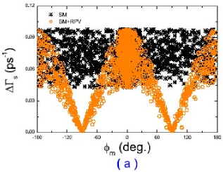
Figure 3: The RPV tree level contributions to the $\Delta\Gamma_{s}$.

Using the constrained parameter space from $\Delta M_{s}$ as shown in Fig.2, one can predict the RPV effects on the $B_{s}$ width difference $\Delta\Gamma_{s}$. Our predictions of $\Delta\Gamma_{s}$ are displayed in Fig.3. From Fig.3(a), we find that $\phi_{m}$ can have any value from $-\pi$ to $\pi$, as discussed in Ref.[18], the RPV contributions to the mixing could reduce $\Delta\Gamma_{s}$ relative to the SM prediction, and $\Delta\Gamma_{s}$ lies between $0.00/\mbox{ps}$ and $0.10/\mbox{ps}$. 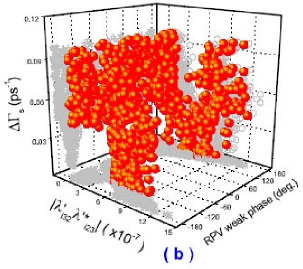We present correlation between $\Delta\Gamma_{s}$ and the parameter space of $\lambda^{\prime}_{i32}\lambda^{\prime*}_{i23}$ by the three-dimensional scatter plot in Fig.3(b). We also give projections on three vertical planes, where the $|\lambda^{\prime}_{i32}\lambda^{\prime*}_{i23}|$-$\phi_{\not\!R_{p}\,}$ plane displays the constrained region of $\lambda^{\prime}_{i32}\lambda^{\prime*}_{i23}$ as the plot of Fig.2. It’s shown that $\Delta\Gamma_{s}$ is decreasing first and then increasing with $|\lambda^{\prime}_{i32}\lambda^{\prime*}_{i23}|$ on the $\Delta\Gamma_{s}$-$|\lambda^{\prime}_{i32}\lambda^{\prime*}_{i23}|$ plane. From the $\Delta\Gamma_{s}$-$\phi_{\not\!R_{p}\,}$ plane, we can see that $\Delta\Gamma_{s}$ may be reduced to zero when $|\phi_{\not\!R_{p}\,}|$ lies in $[\frac{2}{3}\pi,\frac{8}{9}\pi]$.

Figure 4: Allowed parameter space for $\lambda^{\prime}_{i32}\lambda^{\prime*}_{i23}$ constrained by the data of $\Delta M_{s}$ and $\Delta\Gamma_{s}$.

The present experimental data of the $B_{s}$ width difference have a large error, and we obtain the averaged value from [20, 26]

$$\Delta\Gamma_{s}=(0.22\pm 0.09)/\mbox{ps}.$$ (24)

Now we add the experimental constraint of $\Delta\Gamma_{s}$ to the allowed space of $\lambda^{\prime}_{i32}\lambda^{\prime*}_{i23}$. We can not get the solution to the experimental data of $\Delta\Gamma_{s}$ at $1\sigma$ level. If $\Delta\Gamma_{s}$ is varied randomly within $2\sigma$ variance, we can obtain the scatter plot as exhibited in Fig.4. Comparing Fig.4 with Fig.2, we can see that the experimental bound on $\Delta\Gamma_{s}$ shown in Eq.(24) obviously excludes the region $4.4\times 10^{-7}<|\lambda^{\prime}_{i32}\lambda^{\prime*}_{i23}|<5.5\times 10^{-7}$. The stronger limit on $|\lambda^{\prime}_{i32}\lambda^{\prime*}_{i23}|$ from $\Delta M_{s}$ and $\Delta\Gamma_{s}$ than the one from $\Delta M_{s}$ only is obtained

$$|\lambda^{\prime}_{i32}\lambda^{\prime*}_{i23}|\leq 4.4\times 10^{-7}\times\left(\frac{100~{}GeV}{m_{\tilde{\nu}_{i}}}\right)^{2},$$ (25)

and (26)

$$|\lambda^{\prime}_{i32}\lambda^{\prime*}_{i23}|\in[5.5,13.1]\times 10^{-7}\times\left(\frac{100~{}GeV}{m_{\tilde{\nu}_{i}}}\right)^{2}.$$

In summary, we have studied the RPV tree level effects in the $B^{0}_{s}-\bar{B}^{0}_{s}$ mixing with the current experimental measurements. As shown, using the latest experimental data of $\Delta M_{s}$ and the theoretical parameters, we have obtained the allowed space of the RPV coupling product $\lambda^{\prime}_{i32}\lambda^{\prime*}_{i23}$, the upper bound on the magnitude of $\lambda^{\prime}_{i32}\lambda^{\prime*}_{i23}$ has been greatly improved over the existing bounds obtained from the RPV SUSY. Then, we have examined the RPV effects on $\Delta\Gamma_{s}$ by the constrained region of $\lambda^{\prime}_{i32}\lambda^{\prime*}_{i23}$ from $\Delta M_{s}$, and we have found that the RPV contributions to the mixing could reduce $\Delta\Gamma_{s}$ relative to the SM prediction. Finally, using the experimental data of $\Delta M_{s}$ and $\Delta\Gamma_{s}$, we have obtained stronger bound than the one from $\Delta M_{s}$ only on $\lambda^{\prime}_{i32}\lambda^{\prime*}_{i23}$. In addition, we stress that once LHC is turned on, with the anticipated production of $10^{12}$ $b\bar{b}$ per year, the measurements of $\Delta M_{s}$ and $\Delta\Gamma_{s}$ will be much more accurate, then the allowed parameter space for $\lambda^{\prime}_{i32}\lambda^{\prime*}_{i23}$ will be significantly shrunken or ruled out.