Axion results: what is new?

Abstract

The PVLAS collaboration has obtained results that may be interpreted in terms of a light axion-like particle, while the CAST collaboration has not found any signal of such particles. Moreover, the PVLAS results are in gross contradiction with astrophysical bounds. We develop a particle physics model with two paraphotons and with a low energy scale in which these apparent inconsistencies are circumvented.

I Introduction and motivation

Particle physics theories that go beyond the standard $SU(3)\times SU(2)\times U(1)$ model have usually new global symmetries. When one of these global symmetries is spontaneously broken we get a Goldstone or a pseudo Goldstone boson. In general the new particle $\phi$ will be light (or massless) and will couple to two photons. Examples are extensions of the standard model involving breaking of a family symmetry, or lepton number symmetry, or string theories Svrcek:2006yi .

Depending on the parity of the particle the two photon coupling is described by the lagrangian

$${\cal L}_{\phi\gamma\gamma}=\frac{1}{8M}\epsilon_{\mu\nu\rho\sigma}F^{\mu\nu}F^{\rho\sigma}\,\phi$$ (1)

for a pseudoscalar, while for a scalar we would have

$${\cal L}^{\prime}_{\phi\gamma\gamma}=\frac{1}{4M}F_{\mu\nu}F^{\mu\nu}\,\phi$$ (2)

We will denote these new hypothetical light particles by $\phi$, and refer to them as axion-like particles (ALPs) Jaeckel , both for the scalar and pseudoscalar case.

ALP physics has received a lot of attention lately Jaeckel ; nature ; Masso:2005ym ; recentwork ; abel ; Masso:2006gc because ALPs are a plausible explanation of the recent results of the Polarization of Vacuum with Laser (PVLAS) collaboration ZavattiniEM . They observe a rotation of the plane of the polarization of a laser when propagating in a magnetic field. The result can be interpreted as production of an ALP with a mass

$$m\sim 10^{-3}\ {\rm eV}$$ (3)

and a scale interaction

$$M\sim 4\times 10^{5}\ {\rm GeV}$$ (4)

The story is not finished since the coupling (1) or (2) let $\phi$ particles to be produced copiously in the center of our Sun or other stars like red giants. The production mechanism is $\gamma\rightarrow\phi$ in the electromagnetic field of a nucleus or an electron of the star core (this is analogous to the observed Primakoff effect $\gamma\rightarrow\pi^{0}$ in the electromagnetic field of a nucleus). The value (4) is low enough so that the produced ALP escapes the star with no interactions. This would mean a quite large luminosity ${\cal L}_{\phi}$ in this exotic channel. The value (4) implies for the Sun

$${\cal L}_{\phi}\sim 10^{6}\,{\cal L}_{\odot}$$ (5)

Of course, this would be a disaster for the solar evolution.

In these Proceedings we would like to summarize some models that we have developed and where the puzzle is solved. In our models, the coupling (1) or (2) is valid at the very low energies of the PVLAS experiment. However, it gets modified when going to the conditions of the stellar interior. Obviously we look for models where the effective coupling is strongly diminished in the stellar environment. The lagrangians (1) and (2) are five-dimensional operators so that if we wish to get a modification of the coupling we assume a new energy scale of energy much less than the typical stellar interiors, ${\cal O}$(1 keV). Here we will only look at modifications to the $\phi\gamma\gamma$ coupling due to the relatively high temperatures of the Sun. There are other parameters, like the environment density, that also could affect the coupling. This is studied in Jaeckel .

Solving in our way the apparent problem of the PVLAS results when examining its astrophysical consequences, has an additional bonus. There is another puzzle concerning ALPs, that originates in the result of experiment run by the CAST collaboration ZioutasEM . The CAST experiment is a helioscope SikivieEM , which expects to detect the solar flux of $\phi$ particles by means of their conversion in X-rays in a cavity with a strong magnetic field. The null CAST result implies a limit on $M$,

$$M>0.9\times 10^{10}\ {\rm GeV}$$ (6)

The puzzle is clear, (6) and (4) are in gross contradiction. Our models solve also this contradiction, since if we are able to diminish the ALP production in the Sun, then (6) is no longer valid since the CAST bound assumes a standard emission of ALPs.

II Paraphoton Models

Our strategy to lower the novel particle emission from stellar environments is to provide a particular structure to the interactions (1) or (2): a triangle diagram with a new fermion running in the loop (shown in Fig.1). The matching between this diagram and eq.(1) gives

$$\frac{1}{M}=\frac{\alpha}{\pi}\frac{Q_{f}^{2}}{v}$$ (7)

where $Q_{f}$ is the electric charge of $f$ and $v$ is a function of $m_{f}$ and $m_{\phi}$ if $\phi$ has a scalar or pseudoscalar coupling but can be an completely independent energy scale if $\phi$ is a Goldstone boson.

Figure 1: Triangle diagram responsible for the PVLAS signal in our model.

As we want $v$ to be a low energy scale we shall consider models in which $Q_{f}$ is very small. This can be naturally achieved in paraphoton models Holdom:1985ag which can be considered as extensions of QED. The simplest model assumes the addition of new gauge $U(1)_{1}$ symmetry to the usual electromagnetic one which we will call $U(1)_{0}$. As a consequence, the theory has a new gauge boson, $A_{1}$, called paraphoton. Two further ingredients of a typical paraphoton model are fermions that can have electric and/or para-charge and mixing terms $\epsilon F_{0}^{\mu\nu}F_{1\mu\nu}$ between the field strengths $F_{i}^{\mu\nu}$ of the gauge bosons. The later are allowed by the combined symmetry $U(1)_{0}\times U(1)_{1}$ and thus must be present in a renormalizable lagrangian. Furthermore, even if they are not included at the beginning in the theory they are radiatively generated by massive fermions charged under both $U(1)$’s. In what follows we are going to consider that this is the case, so small values of $\epsilon$ are natural on the basis of their radiative origin.

The important point is that these mixing terms act as if there where new contributions to the fermion charges $Q_{i}$. This can be explained in several ways. In Masso:2005ym we use one of them first presented in Holdom:1985ag that consists in diagonalizing together the kinetic and mass parts of the lagrangian for the gauge bosons. Let us develop here a simpler (though less formal) method of calculation.

In the LHS of Fig.2 we see the interaction of a para-fermion $f$ belonging to the representation $(0,Q_{1}^{f})$ with an electron $\in(Q_{0}^{e},0)$. We consider the general case in which both gauge bosons are massive. The value of this amplitude is

$${\cal A}=(e_{0}Q^{e}_{0}j^{e}_{\mu})\frac{i}{q^{2}-m_{0}^{2}}(\epsilon iq^{2})\frac{i}{q^{2}-m_{1}^{2}}(e_{1}Q^{f}_{1}j^{f\mu})$$ (8)

($q$ is the momentum carried by the bosons, $e_{0},e_{1}$ are the coupling constants and $j_{\mu}^{e},j_{\mu}^{f}$ the currents of electrons and $f$ particles) which we can decompose using

$$\frac{-iq^{2}}{(q^{2}-m_{0}^{2})(q^{2}-m_{1}^{2})}=\frac{m_{0}^{2}}{m_{1}^{2}-m_{0}^{2}}\frac{i}{q^{2}-m_{0}^{2}}+\frac{m_{1}^{2}}{m_{0}^{2}-m_{1}^{2}}\frac{i}{q^{2}-m_{1}^{2}}$$ (9)

to realize that this amplitude is completely equivalent to the sum of two single boson exchange diagrams as shown in Fig.2 which require that we assign an $\epsilon$-charge to $f$ and a $\epsilon$-para-charge to the electron $e$:

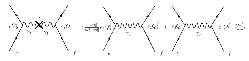
Figure 2: Mixing between massive photons is equivalent to new $\epsilon$-charges for the fermions.

$$Q_{0}^{f}=\epsilon Q_{1}^{f}\frac{m_{0}^{2}}{m_{1}^{2}-m_{0}^{2}}\frac{e_{1}}{e_{0}}\hskip 28.45274ptQ_{1}^{e}=\epsilon Q_{0}^{e}\frac{m_{1}^{2}}{m_{0}^{2}-m_{1}^{2}}\frac{e_{0}}{e_{1}}$$ (10)

These charges are in agreement with eq.(15) of Masso:2005ym which was derived by a different method. Note in particular that if a boson is massless and the other massive, only particles that coupled to the massless boson acquire new charges. A final remark is worth, namely that we are adjusting the charges by comparing diagrams in perturbation theory and clearly when the photons are degenerate in mass the charges diverge so our formulae do not hold for the case $m_{0}=m_{1}\neq 0$. Interestingly enough they can be useful for the case in which the two bosons are massless because we can fulfill the perturbative condition by performing first the limit $m_{0}\rightarrow 0$ and after $m_{1}\rightarrow 0$ or viceversa. The result is shocking at first sight: the two orderings give different assignments of charge! To understand that this is not an inconsistency let us show the value of the $ef\rightarrow ef$ amplitude in this case:

$${\cal A}=(e_{0}Q^{e}_{0}j^{e}_{\mu})\frac{i}{q^{2}}(\epsilon iq^{2})\frac{i}{q^{2}}(e_{1}Q^{f}_{1}j^{f\mu})=(e_{0}Q^{e}_{0}j^{e}_{\mu})\frac{-i\epsilon}{q^{2}}(e_{1}Q^{f}_{1}j^{f\mu})$$ (11)

We see that this amplitude could be attributed to diagram with exchange of a $\gamma_{0}$ an a new $\epsilon$-sized $Q_{0}^{f}$

$$Q_{0}^{f}=-\epsilon Q_{1}^{f}e_{1}/e_{0}$$ (12)

or to a diagram with exchange of $\gamma_{1}$ and a $\epsilon$-sized $Q_{1}^{e}$:

$$Q_{1}^{e}=-\epsilon Q_{0}^{e}e_{0}/e_{1}$$ (13)

Indeed, generally we can put a combination of both such that the sum remains the same. This would correspond to take the limit $m_{0}^{2}=\alpha m_{1}^{2}\rightarrow 0$ in eq.(10) (with $|\alpha-1|\gg\epsilon$) which gives:

$$Q_{0}^{f}=\epsilon Q_{1}^{f}\frac{1}{\alpha-1}\frac{e_{1}}{e_{0}}\hskip 28.45274ptQ_{1}^{e}=\epsilon Q_{0}^{e}\frac{\alpha}{1-\alpha}\frac{e_{0}}{e_{1}}$$ (14)

This freedom in the assignment of charges can be traced back to the freedom we have to rotate the basis $\{A_{0},A_{1}\}$ because the photons are degenerated in mass as we comment in Masso:2005ym . We find then that in this case the $\epsilon$-charge assignments are convention dependent.

Now that we can calculate easily charges arising from mixing terms in paraphoton models we are going to apply our knowledge to explain our solution to the PVLAS-CAST apparent inconsistency.

II.1 A model with two paraphotons solving the PVLAS-CAST inconsistency

The motivation of our model comes from the high $q^{2}$ behavior of the LHS diagram in Fig.2 shown in (8). As we go higher in $q^{2}$ the dependence on the paraphoton mass $m_{1}$ becomes smaller. Then we can consider that in adition to the amplitude of Fig.2 we have other diagram with a different paraphoton $\gamma_{2}$ with different mass $m_{2}$ that, having opposite sign, cancels the first one at high $q^{2}$ (corresponding to the typical stellar environment) but leaves a finite contribution at low $q^{2}$ where the PVLAS experiment takes place.

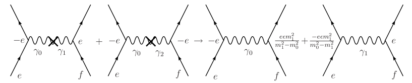
Figure 3: $ef\rightarrow ef$ from which we can infer the charges in our paraphoton model. We have set $e_{0}=e_{1}=e_{2}=e$, $Q_{0}^{e}=-1$, $Q_{1}^{f}=-Q_{2}^{f}=1$. The two LHS diagrams are equivalent to the two RHS. The diagram of the $\gamma_{0}$ exchange recieves contributions from $\gamma_{0}-\gamma_{1}$ and $\gamma_{0}-\gamma_{2}$ mixing diagrams that cancel at high $m_{0}$, while the later is due only to $\gamma_{0}-\gamma_{1}$.

We consider then a model with two paraphotons in which the local symmetry is $U(1)_{0}\otimes U(1)_{1}\otimes U(1)_{2}$. The condition that we have to impose for the two diagrams to cancel at high momentum transfer is $\epsilon_{01}e_{1}Q_{1}^{f}-\epsilon_{02}e_{2}Q_{2}^{f}=0$ as can be deduced from Fig.3. We can set $e_{0}=e_{1}=e_{2}$ for simplicity. Very massive fermions $F$ in the representations $(Q_{0}^{F},Q^{F},Q^{F})$ will produce naturally $\epsilon_{01}=\epsilon_{02}$ and we can choose $Q_{1}^{f}=-Q_{2}^{f}=1$ for the light para-fermion $f$. The second condition is that at the low momentum transfer of the PVLAS experiment ($q^{2}\sim 10^{-6}$ eV²) $Q_{0}^{f}$ should be finite and preferably maximum. Note from (10) that massive paraphotons imply $Q_{0}^{f}=0$ when photons are in vacuum ($m_{0}=0$), so we need one paraphoton to be massless. Accordingly we choose $m_{1}=\mu\neq 0$ and $m_{2}=0$. We must, however, note that in the sun the dispersion relation of photons resembles that of a massive particle with mass equal to the plasma frequency so $m_{0}=\omega_{P}\sim 4\pi\alpha n_{e}/m_{e}$ ($\alpha\sim 1/137$, while $n_{e}$ and $m_{e}$ are the electron density and mass, respectively). Then we find that the electric charge of $f$ depends on the environment where it is probed, and from (12) and (10) we get:

$$Q_{0}^{f}(PVLAS)=\epsilon\hskip 28.45274pt;\hskip 28.45274ptQ_{0}^{f}(Sun)\sim-\epsilon\frac{\mu^{2}}{\omega_{P}^{2}}$$ (15)

We reach our goal of having a decrease of the electric charge of $f$ and consequently of the novel particle emission from the sun by requiring $\mu/\omega_{P}$ to be small enough.

II.2 Astrophysical bounds evaded

We now discuss the consequences of our model. The PVLAS experiment is in vacuum, so $f$ has an effective electric charge $Q^{f}_{0}=\epsilon$, which from (1) has to be

$$\epsilon^{2}\simeq 10^{-12}\,\frac{v}{\rm eV}$$ (16)

Concerning the astrophysical constraints Raffelt:1996wa we should first look for the relevant production processes of the exotic particles in our model. We notice that the amplitude for the Primakoff effect $\gamma Z\rightarrow\phi Z$ is of order $\epsilon^{2}(\mu^{2}/\omega_{P}^{2})^{2}$. But there are production processes with amplitudes of order $\epsilon(\mu^{2}/\omega_{P}^{2})$ which will be more effective. The most efficient is plasmon decay $\gamma^{*}\rightarrow\bar{f}f$. Energy loss arguments in horizontal-branch (HB) stars Davidson:1991si limits $Q_{0}^{f}<2\times 10^{-14}$, which translates in our model into the bound

$$\epsilon\ \frac{\mu^{2}}{\rm eV^{2}}<4\times 10^{-8}$$ (17)

(we have introduced $\omega_{P}\simeq 2$ keV in a typical HB core). But equations (16) and (17) do not fully determine the parameters of our model. Together they imply the constraint

$$v\,\mu^{4}<(\,0.4\ {\rm eV})^{5}$$ (18)

We can now make explicit one of our main results. In the reasonable case that $v$ and $\mu$ are not too different, we wee that the new physics scale is in the sub eV range.

On the other hand, the CAST telescope is able to detect $\phi$’s with energies within $1$ and $14$ keV. In our model, $f$’s and paraphotons are emitted from the Sun, but we should care about $\phi$ production. We consider three possibilities.

A) $\phi$ is a fundamental particle. Production takes place mainly through plasmon decay $\gamma^{*}\rightarrow\bar{f}f\phi$. The $\phi$-flux is suppressed, but, most importantly, the average $\phi$ energy is much less than $\omega_{P}\simeq.3$ keV, the solar plasmon mass. The spectrum then will be below the present CAST energy window.

B) $\phi$ is a composite $\bar{f}f$ particle confined by new strong confining forces. The final products of plasmon decay would be a cascade of $\phi$’s and other resonances which again would not have enough energy to be detected by CAST citaK .

C) $\phi$ is a positronium-like bound state of $\bar{f}f$, with paraphotons providing the binding force. As the binding energy should be small, ALPs are not produced in the solar plasma.

A final constraint should bother us. In vacuum, $\gamma_{1}$ couples to electrons with a strength $\epsilon$ and a range $\mu^{-1}$ and this interaction is limited by Cavendish-type experiments Bartlett:1988yy .

Finally, in Fig.(4) we show all these limits. In the ordinates we can see both $\epsilon$ and $v$, since we assume they are related by (16). We find out that there is wide room for the parameters of our model, even in the natural line $v=\mu$ or further, in the preferred point $v=m_{f}=m_{\phi}\sim$ meV.

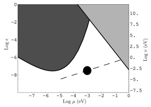
Figure 4: Constraints on the parameters of our model. The black area is excluded by Cavendish-type experiments, and the grey area by the astrophysical constraint (17). The dashed line corresponds to $v=\mu$, and the dot to $v=\mu\simeq 1$ meV.

To conclude let us say that the PVLAS-CAST puzzle has recently received very much attention. We have presented a model with two paraphotons and a new fermion $f$ living all at a low energy scale, below eV, in which the apparent discrepancy is safely circumvented. Let us also mention that recently our model has been justified in the context of string theory abel .

III Acknowledgments

We acknowledge support by the projects FPA2005-05904 (CICYT) and 2005SGR00916 (DURSI).

References

- (1) P. Svrcek and E. Witten, JHEP 0606, 051 (2006) [arXiv:hep-th/0605206]; P. Svrcek, [arXiv:hep-th/0607086].
- (2) J. Jaeckel, E. Masso, J. Redondo, A. Ringwald and F. Takahashi, [arXiv:hep-ph/0605313], and in preparation.
- (3) S. Lamoreaux, Nature 441, 31 - 32 (2006).
- (4) E. Masso and J. Redondo, JCAP 0509, 015 (2005) [arXiv:hep-ph/0504202].
- (5) P. Jain and S. Mandal, [astro-ph/0512155]; C. Biggio, E. Masso and J. Redondo, [arXiv:hep-ph/0604062]; I. Antoniadis, A. Boyarsky and O. Ruchayskiy, [arXiv:hep-ph/0606306]; H. Gies, J. Jaeckel and A. Ringwald, [hep-ph/0607118]; T. Fukuyama and T. Kikuchi, [arXiv:hep-ph/0608228];
- (6) S. A. Abel, J. Jaeckel, V. V. Khoze and A. Ringwald, [hep-ph/0608248].
- (7) E. Masso and J. Redondo, [arXiv:hep-ph/0606163], accepted for publication in Phys. Rev. Lett..
- (8) E. Zavattini et al. [PVLAS Collaboration], Phys. Rev. Lett. 96, 110406 (2006) [arXiv:hep-ex/0507107]
- (9) K. Zioutas et al. [CAST Collaboration], Phys. Rev. Lett. 94, 121301 (2005) [arXiv:hep-ex/0411033]
- (10) P. Sikivie, Phys. Rev. Lett. 51, 1415 (1983) [Erratum-ibid. 52, 695 (1984)]
- (11) B. Holdom, Phys. Lett. B 166, 196 (1986), ibid. 178, 65 (1986); L. B. Okun, Sov. Phys. JETP 56, 502 (1982) [Zh. Eksp. Teor. Fiz. 83, 892 (1982)].
- (12) For a complete description see: G. G. Raffelt, “Stars as laboratories for fundamental physics”, Chicago Univ. Pr. (1996).
- (13) S. Davidson, B. Campbell and D. Bailey, Phys. Rev. D 43, 2314 (1991); S. Davidson and M. Peskin, Phys. Rev. D 49, 2114 (1994) [arXiv:hep-ph/9310288]; S. Davidson, S. Hannestad and G. Raffelt, JHEP 0005, 003 (2000) [arXiv:hep-ph/0001179].
- (14) For a model of composite see Masso:2005ym .
- (15) E. R. Williams, J. E. Faller and H. A. Hill, Phys. Rev. Lett. 26, 721 (1971); D. F. Bartlett and S. Logl, Phys. Rev. Lett. 61, 2285 (1988).