Radiative B decay spectrum: DGE at NNLO

Abstract:

We compute the differential $\bar{B}\to X_{s}\gamma$ decay width in the Standard Model as a function of the photon energy using Dressed Gluon Exponentiation (DGE). The resummed spectrum is matched with the fixed–order expansion, making use of the next–to–next–to–leading order (NNLO) results for the matrix element of the magnetic dipole interaction $O_{7}$ and NLO ones for other operators in the effective Weak Hamiltonian. We develop a new technique to implement constraints on the analytic structure of the Sudakov factor in moment space. This improves the behavior of the resummed spectrum away from the Sudakov region. We also derive an analytic expression for the Borel transform of the perturbative series for the $O_{7}$ spectrum in the large–$\beta_{0}$ limit. Using this example we demonstrate that exponentiation in moment space is necessary for the calculation of the spectrum for $E_{\gamma}\mathrel{\mathchoice{\vbox{\offinterlineskip\halign{$\m@th\displaystyle\hfil#\hfil$\cr>\crcr\sim\crcr} }}{\vbox{\offinterlineskip\halign{$\m@th\textstyle\hfil#\hfil$\cr>\crcr\sim\crcr} }}{\vbox{\offinterlineskip\halign{$\m@th\scriptstyle\hfil#\hfil$\cr>\crcr\sim\crcr} }}{\vbox{\offinterlineskip\halign{$\m@th\scriptscriptstyle\hfil#\hfil$\cr>\crcr\sim\crcr} }}}2$ GeV. Finally, we investigate numerically the relation between renormalons, power corrections and support properties. We present predictions for the branching fraction and the first few spectral moments as a function of a cut $E_{\gamma}>E_{0}$ and estimate the theoretical uncertainty.

1 Introduction

Inclusive radiative B decays, $\bar{B}\longrightarrow X_{s}\gamma$, have become an essential ingredient in precision tests of the Standard Model. The Standard Model $b\to s\gamma$ decay occurs only through loops (penguin diagrams) involving the W Boson, whose mass is significantly larger than the available energy, $m_{W}\gg m_{b}$. This makes the $\bar{B}\longrightarrow X_{s}\gamma$ width a sensitive probe of any potential flavor–changing short–distance interaction beyond the Standard Model, see e.g. [1, 2, 3].

The Standard Model Branching Fraction (BF) is known [4, 5, 6, 7, 8] since a few years to next–to–leading order (NLO) in renormalization–group improved perturbation theory. The summation of large logarithms of $m_{b}/m_{W}$ is conveniently formulated in the framework of the effective Weak Hamiltonian, where virtualities of order of the Weak scale are integrated out to obtain a set of local operators $O_{i}$ of dimension 6. The result for the inclusive decay width with a minimal photon–energy cut, $E_{\gamma}>E_{0}$, takes the form:

$$\Gamma(\bar{B}\longrightarrow X_{s}\gamma,E>E_{0}) = \frac{\alpha_{\rm em}G_{F}^{2}}{32\pi^{4}}\left|V_{\rm tb}V_{\rm ts}^{*}\right|^{2}\,\left(m_{b}^{\hbox{\tiny${\overline{\rm MS}}$}}(m_{b})\right)^{2}\,m_{b}^{3}\,$$

$$\hskip 60.0pt\times\,\sum_{i,j,\,i\leq j}C^{\hbox{\tiny eff}}_{i}(\mu)C_{j}^{\hbox{\tiny eff}}(\mu)\,{G_{ij}(E_{0},\mu)},$$

where $m_{b}$ is the quark pole mass, $G_{ij}(E_{0},\mu)$ are matrix elements of operators in the effective Weak Hamiltonian, $G_{ij}(E_{0},\mu)=\sum_{X_{s}}\left<\bar{B}\right|O_{i}^{\dagger}(\mu)\left|X_{s}\gamma\right>\left<X_{s}\gamma\right|O_{j}(\mu)\left|\bar{B}\right>$ where $E_{\gamma}>E_{0}$, and $C^{\hbox{\tiny eff}}_{i}(\mu)$ are the corresponding Wilson coefficients. The matrix elements can be computed in perturbation theory, replacing the $\bar{B}$ meson by an on-shell b quark and the hadronic system $X_{s}$ by a partonic one, owing to the inclusive sum over the final states. This replacement can be justified using the Operator Product Expansion (OPE) so long as the photon–energy cut is insignificant. Upon removing the cut, power corrections to the partonic calculation can be formally shown to be of ${\cal O}(\Lambda^{2}/m_{b}^{2})$, and they are numerically small, approximately $+2.5\%$ of the total BF [7]. The Standard Model BF, which has been determined with about $\pm 10\%$ uncertainty [7, 8], is found to be in good agreement with experimental measurements by CLEO, Belle and BaBar [9, 10, 11, 12, 13, 14].

The current world average of all experimental data, prepared by the Heavy Flavor Averaging Group [15], is ${\cal B}(\bar{B}\longrightarrow X_{s}\gamma,E_{\gamma}>1.6\,{\rm GeV})=(355\pm 24\pm 10\pm 3)\times 10^{-6}$, where the errors are: combined statistical and systematic uncertainty, “shape–function” uncertainty owing to the extrapolation from the region of measurement $E_{\gamma}>E_{0}$, where $E_{0}\geq 1.8\,{\rm GeV}$, to the reference range of $E_{\gamma}>1.6\,{\rm GeV}$, and uncertainty owing to the $b\to d\gamma$ fraction. The “shape–function” uncertainty varies significantly between different theoretical approaches. For example, Ref. [16] assigns an error of about $\pm 8\%$ to the extrapolation below $E_{0}=1.8$ GeV, i.e. three times the size of the error quoted here.

One of the essential ingredients for improving the precision of this comparison in the future is the theoretical calculation of the photon energy spectrum. Owing to irreducible background, experimental measurements are limited to the range $E_{\gamma}>1.8\,{\rm GeV}$ and they can be significantly improved if the requirement on the range of measurement is relaxed, for example, to $E_{\gamma}>2.0\,{\rm GeV}$. This, however, requires larger extrapolation that relies on the theoretical description of the spectrum. Fortunately, this extrapolation presents very little sensitivity to short–distance physics, in sharp contrast with the total width. On the other hand, it requires detailed understanding of the QCD dynamics.

The QCD calculation of inclusive decay spectra is essential for other aspects of flavor physics. An important example is the determination of $|V_{\rm ub}|$ from inclusive charmless semileptonic decays, $\bar{B}\longrightarrow X_{u}l\bar{\nu}$, where the background due to the $50$ times more abundant semileptonic decay into charm restricts the region of measurement to $M_{X}<1.7$ GeV. The dynamics there is similar to the one governing the $\bar{B}\longrightarrow X_{s}\gamma$ spectrum to the extent that spectral measurements of the photon–energy spectrum in $\bar{B}\longrightarrow X_{s}\gamma$ are used for the determination of $|V_{\rm ub}|$. In recent years the $\bar{B}\longrightarrow X_{s}\gamma$ spectrum has become the prime testing–grounds for theoretical approaches to inclusive distributions, see e.g. [17, 18, 19, 20, 21, 22, 23, 24, 25, 26, 16, 27, 28, 29].

The main challenge in computing inclusive decay spectra in QCD is the complex dynamics of the threshold region. In this region the decaying b quark is just slightly off its mass shell, owing to its “primordial” Fermi motion and to soft gluon radiation [30, 31, 32, 33]. Specifically, the $\bar{B}\longrightarrow X_{s}\gamma$ spectrum peaks near the partonic threshold, $E_{\gamma}\longrightarrow m_{b}/2$, or $x\equiv 2E_{\gamma}/m_{b}\longrightarrow 1$. This region is characterized by parametrically–large higher–order perturbative corrections (Sudakov logs) [33] as well as non-perturbative effects, predominantly ones related to the Fermi motion of the b quark in the B meson.

It is universally acknowledged that fixed–order perturbative results cannot be directly used for comparison with spectral data, not even the first few moments of the photon energy with experimentally–relevant cuts, such as $E_{\gamma}>1.8$ GeV. Fixed–order results for the $\bar{B}\longrightarrow X_{s}\gamma$ spectrum are characterized by

• Sudakov logarithms, namely singular real-emission corrections to the differential spectrum ${d\Gamma(x)}/{dx}$, of the form $\ln^{k}(1-x)/(1-x)$ with $k\leq 2n-1$ at order ${\alpha_{s}}^{n}$, owing to multiple soft and collinear radiation. The perturbative spectrum is nevertheless integrable as there are also infrared–singular virtual corrections proportional to $\delta(1-x)$ — the spectral moments,

  $$\Gamma_{N}^{\hbox{\tiny PT}}\equiv\int_{0}^{1}dx\,\frac{1}{\Gamma_{\hbox{\tiny total}}^{\hbox{\tiny PT}}}\frac{d\Gamma^{\hbox{\tiny PT}}(x)}{dx}\,x^{N-1}$$ (2)

  are infrared safe.

• Support for $E_{\gamma}<m_{b}/2$, where $m_{b}$ is the quark pole mass, setting the upper limit of integration in Eq. (2) as $x=1$. The perturbative support at any order is different from the physical one, $E_{\gamma}<M_{B}/2$, where $M_{B}$ is the meson mass. Importantly, the pole mass itself has a linear infrared renormalon ambiguity [34, 35, 36], $m_{b}\to m_{b}\pm{\cal O}(\Lambda)$, and therefore it cannot be assigned a precise value without specifying an additional regularization prescription. In a fixed–order framework one computes the pole mass order-by-order from a given short–distance mass, such as $m_{b}^{\hbox{\tiny${\overline{\rm MS}}$}}$, but the result strongly depends on the order, as the series is badly divergent. The use of alternative mass schemes [26, 27, 37, 38] amounts to introducing an infrared cutoff, which hinders the possibility of using of the inherent infrared safety of the on-shell decay spectrum.

• Large running–coupling effects, which completely dominate the NNLO correction to the spectrum [39] if the coupling at NLO is renormalized at $m_{b}$. Large running–coupling effects reflect the fact that the typical gluon virtuality is much smaller than $m_{b}$. Naturally, large running–coupling corrections appear also at higher orders. Real-emission corrections proportional to $C_{F}\beta_{0}^{n-1}{\alpha_{s}}^{n}$, where $\beta_{0}$ (20) is the leading coefficient of the beta function, were computed in [18] to all orders. In Sec. 2.3 below we will show that the series composed of these terms alone (i.e. with no exponentiation, no effect of real–virtual cancellation) cannot be considered a viable prediction for the spectrum anywhere in the peak region. This series is Borel summable up to $E_{\gamma}\sim 2$ GeV, but ceases to be so above this scale, where the Borel integral diverges for $u\longrightarrow\infty$.

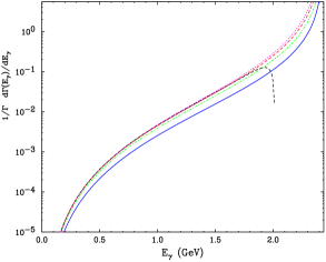
The numerical results for the spectrum obtained by fixed–order calculations at NLO and NNLO, as well as running–coupling corrections beyond this order, are shown in Fig. 1, with the pole mass is set to $m_{b}=4.89$ GeV. The lack of convergence in the peak region is apparent.

Figure 1: Comparison between the differential spectra for $\bar{B}\longrightarrow X_{s}\gamma$ decay (through $O_{7}$ only) obtained by DGE, matched to NLO or NNLO, with fixed–order results in $E_{\gamma}$ space ($x$ space). All curves correspond to the same value of the b-quark mass, the PV pole mass $m_{b}=4.89$ GeV. The end of partonic phase space, $E_{\gamma}=m_{b}/2$, is denoted by an arrow.

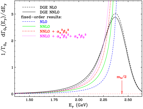
These characteristics of the fixed–order result point towards the necessity for (1) resummation of all large perturbative corrections (2) systematic separation between perturbative and non-perturbative contributions and appropriate parametrization of the latter. Dressed Gluon Exponentiation (DGE) offers a framework to do so, utilizing directly the on-shell scheme [18, 40, 17]. Owing to its inherent infrared safety, the on-shell decay spectrum itself provides then a first approximation to the physical B–meson decay spectrum. Fig. 1 shows these results as well. Other approaches to compute the spectrum [29, 16, 27] have been based on introducing an infrared cutoff as means of separation between perturbative and non-perturbative corrections. With a cutoff in place, a first approximation to the B–meson decay spectrum is obtained only upon convoluting the perturbative result with a leading–power non-perturbative quark distribution function, or “shape function” [30, 31, 32, 33, 25, 26, 27, 37, 38]. Ref. [17] has shown that a cutoff and a leading–power “shape function” can be avoided, and replaced by a resummation of the perturbative expansion, a prescription for the renormalon singularities (Principal Value of the Borel sum) and power corrections. This involves of course making certain assumptions on the perturbative expansion and on non-perurbative corrections. Aside from the separation issue, the calculation in Ref. [17] applies a novel approach to resummation per se. Different higher–order corrections are considered important in different approaches:

• Refs. [16, 27] emphasize the significance of Sudakov logarithms and utilize a logarithmic accuracy criterion and an infrared cuoff.

• Ref. [29] emphasizes the significance of running–coupling corrections (dismissing Sudakov logarithms) and utilizes large–$\beta_{0}$ resummation with a Wilsonian cutoff.

• Ref. [17] resums Sudakov logarithms as well as running–coupling corrections in the Sudakov exponent and utilizes additional information on the Borel transform of the exponent to complement the logarithmic accuracy criterion.

Upon resumming the perturbative expansion for the matrix elements $G_{ij}$ as a function of the cut $E_{0}$, normalized by $G_{ij}(E_{\min})$, Eq. (1) can be written as:

$$\Gamma(\bar{B}\longrightarrow X_{s}\gamma,E>E_{0}) = \frac{\alpha_{\rm em}G_{F}^{2}}{32\pi^{4}}\left|V_{\rm tb}V_{\rm ts}^{*}\right|^{2}\,\left(m_{b}^{\hbox{\tiny${\overline{\rm MS}}$}}(m_{b})\right)^{2}\,m_{b}^{3}\,$$

$$\times\,\sum_{i,j,\,i\leq j}C^{\hbox{\tiny eff}}_{i}(\mu)C_{j}^{\hbox{\tiny eff}}(\mu)\,{G_{ij}(E_{\min},\mu)}\left[\frac{G_{ij}(E_{0})}{G_{ij}(E_{\min})}\right]_{\rm Resummed},$$

where it is assumed that $E_{\min}\ll m_{b}/2$ so $G_{ij}(E_{\min},\mu)$ can be computed using fixed–order perturbation theory (our choice will be $E_{\min}=m_{b}/20$) while $E_{0}$ can take any value, in particular, experimentally–relevant one: $E_{0}\geq 1.8$ GeV.

The essential element in the calculation of resummed spectra near threshold, namely $\left[{G_{ij}(E_{0})}/{G_{ij}(E_{\min})}\right]_{\rm Resummed}$ in Eq. (1), is the Sudakov factor, which sums up the dominant corrections owing to multiple soft gluon emission that exponentiate in moment space. In DGE the Sudakov exponent is computed as Borel sum, combining Sudakov resummation with the resummation of running–coupling effects. This immediately exposes the power–like infrared sensitivity of the on-shell matrix elements in the form of renormalons. This allows for

• Explicit cancellation of the leading renormalon ambiguity, the one associated with the definition of the pole mass.

• Definite regularization of all renormalons, using the Principal Value prescription.

This definition of the perturbative sum amounts to a systematic separation between perturbative and non-perturbative corrections. This procedure uniquely defines the non-perturbative Fermi motion effect, distinguishing it from the radiation effect that is common to an on-shell heavy quark and to one that is part of a meson. As already mentioned, in contrast with other formulations, no infrared cutoff is needed here. Therefore, Fermi motion effects enter exclusively through power corrections. These power corrections are power–enhanced at large $N$: they scale as powers of $N\Lambda/m_{b}$, so they can modify the perturbative on-shell spectrum by ${\cal O}(1)$ corrections near threshold while almost not affecting the first few moments and the distribution away from threshold. According to the renormalon structure of the exponent, non-perturbative corrections start at the third power of $N\Lambda/m_{b}$, making just a small correction to the spectrum. The numerical significance of these power corrections will be analyzed in Sec. 4 below.

As shown in Fig. 1 the DGE spectrum is qualitatively different from the fixed–order results. It is characterized by

• Approximate physical support: the spectrum smoothly extends beyond the perturbative endpoint, $E_{\gamma}=m_{b}/2$, and tends to zero close to the physical one, $E_{\gamma}=M_{B}/2$.

• Mass–scheme independence, owing to the explicit cancellation of the pole–mass rerormalon ambiguity.

• Stability in going from order to order, reflecting the fact that the dominant higher–order corrections are indeed resummed.

The DGE $\bar{B}\longrightarrow X_{s}\gamma$ spectrum, and its first few moments with experimentally relevant cuts, were computed in Ref. [17]. Later, when experimental data for the average energy the variance appeared [14, 12, 13], these predictions where found to be in good agreement [41, 19].

Recently there has been significant progress in higher–order calculations. The NNLO corrections to the spectrum associated with the matrix element $G_{77}(E_{0})$ of the magnetic dipole operator

$$O_{7}\equiv\frac{\,e}{32\pi^{2}}\,m_{\hbox{\tiny${\overline{\rm MS}}$}}\,F^{\mu\nu}\,\,\bar{s}\,\sigma_{\mu\nu}(1+\gamma_{5})\,b$$ (4)

have been computed in full [39, 42]. The resummed spectrum of Ref. [17] already included NNLL corrections through the Sudakov factor [17, 43]; however, it included non-logarithmic corrections to NLO only. One of the tasks of the present paper is to match the resummed spectrum to full NNLO accuracy in the $O_{7}$ sector. We also consider other operators in the Weak Hamiltonian, which have been so far computed to ${\cal O}(\alpha_{s})$ only. Knowing that independently of the nature of the short–distance interaction, all important contributions in the peak region necessarily involve the same Sudakov factor, we compute resummed spectra for individual matrix elements $G_{ij}(E_{0})$, determining the hard coefficient functions at ${\cal O}(\alpha_{s})$ from known results.

In addition, significant progress towards NNLO calculation of the total BF was recently made [44, 45]: two–loop matrix element of the $O_{7}$ operator have been computed in full. This adds to the already existing NNLO results in the framework of the effective Weak Hamiltonian, which includes the matching coefficients at the Weak scale [46], partial information on the evolution matrix [47, 48], as well as $\beta_{0}{\alpha_{s}}^{2}$ contributions to $\bar{B}\longrightarrow X_{s}\gamma$ of several matrix elements [49]. It is our aim here to set a framework where the state-of-the-art calculation of the spectrum can be used together with that of the total BF. This would be particularly important once the NNLO calculation is complete. A detailed knowledge of the partial BF as a function of the photon–energy cut $E_{\gamma}>E_{0}$ can help making good use of the data, since low cuts, such as $E_{0}=1.8$ GeV, are characterized by large systematic experimental errors, in contrast with higher cuts, such as $E_{0}=2.0$ GeV, that, in turn, requires larger extrapolation.

An important new ingredient in the calculation of the spectrum that we develop in this paper is the use of the analytic structure of the perturbative result in moment space when writing the resummation formula. It is a general problem in the application of Sudakov resummation, that the region of interest may extend far beyond the asymptotic Sudakov regime where the logs are large and the coupling is small. An immediate implication is that the resummed result depends on the (often implicit) assumptions made concerning non-logarithmic ${\cal O}(1/N)$ higher–order corrections. Non-logarithmic corrections are of course included to some fixed order in ${\alpha_{s}}$ in the process of matching the resummed spectrum into the fixed–order expansion. This procedure, however, may not be sufficient to avoid bias of the result due to the resummation of logarithms in the region where the logarithms are not at all dominant.

The $\bar{B}\longrightarrow X_{s}\gamma$ spectrum provides an important motivation to address this problem, since the region where the logarithms alone dominate is rather small, at least up to the NNLO level [39]. To make good use of perturbation theory it is therefore important to impose additional constrains on the resummation formula. Such constraints are indeed available: the analytic structure of the perturbative result (at any order) in moment space is known fairly well: perturbative coefficients are composed of harmonic sums and rational functions whose singularities appear on the negative real axis in $N$ space. The rightmost singularity appears at $N=-J$ where $J$, a non-negative integer, corresponds to the power fall of the spectrum, $d\Gamma/dx\sim x^{J}$, in the $x\to 0$ limit. In $\bar{B}\longrightarrow X_{s}\gamma$, for most matrix elements, $J=3$. Thus, there is quite a strong suppression of the spectrum at small $x$, which obviously would not be respected by a generic large–$x$ resummation formula that accounts only for $\ln^{l}(1-x)/(1-x)$ terms. A power fall is generally expected when the $x\to 0$ behavior is dominated by phase space.

The remainder of this paper is organized as follows: Sec. 2 is devoted entirely to the normalized spectrum of the $G_{77}$ matrix element, corresponding to the magnetic dipole operator, $O_{7}$. $G_{77}$ is the only matrix element contributing at ${\cal O}(1)$, while other $G_{ij}$ start at ${\cal O}({\alpha_{s}})$. Moreover, $G_{77}$ is the only matrix element for which the full ${\cal O}({\alpha_{s}}^{2})$ (NNLO) result is available [39, 42, 44, 45]. This facilitates matching of the resummed spectrum to NNLO as well as performing an in-depth analysis of the perturbative expansion. In Sec. 2.1 we briefly summarize the main assumptions and the necessary formulae in the application of DGE to the radiative B decay spectrum. In Sec. 2.2 we reformulate the resummation formulae under constraints on the analytic structure in moment space, in order to have a good description of the small $E_{\gamma}$ tail. Next, in Sec. 2.3 we analyze the all–order result in the large–$\beta_{0}$ limit. Sec. 3 is devoted to computing the resummed spectra for the matrix elements $G_{ij}$ other than $G_{77}$. In Sec. 4 we compute the total BF and incorporate the resummed spectra of Secs. 2 and 3 into Eq. (1), to obtain the BF as a function of $E_{0}$. We also study there numerically the relation between renormalons, power correction and support properties. Finally, we present predictions for the first few moments as a function of the cut and analyze the theoretical uncertainty. In Sec. 5 we shortly summarize our conclusions.

2 Resummed spectrum for the magnetic dipole operator $O_{7}$ 

2.1 Dressed Gluon Exponentiation 

DGE is a general resummation formalism for inclusive distributions that is designed to address kinematic threshold problems in QCD where there is interplay between Sudakov logarithms, running–coupling effects and parametrically–enhanced power corrections. The formalism will not be described here in any detail; we refer the reader to a recent review [40]. Here we concentrate on the application to $\bar{B}\longrightarrow X_{s}\gamma$ [17], briefly summarizing the main assumptions and the necessary formulae.

For simplicity we consider in this section the normalized spectrum associated with the magnetic dipole operator only, postponing the calculation of the spectra of other matrix elements to Sec. 3, and the calculation of the overall normalization of the BF to Sec. 4, where the contributions of the different matrix elements are combined with the appropriate Wilson coefficients.

Formulating Sudakov resummation in moment space

The normalized differential spectrum associated with the magnetic dipole operator takes the form

$$\begin{split}\frac{1}{\Gamma_{O_{7}}}\,\frac{d\Gamma_{O_{7}}(x)}{dx}&=V\left(\alpha_{s}(m_{b})\right)\,\delta(1-x)\,+\,R\left(\alpha_{s}(m_{b}),x\right),\\ &V\left(\alpha_{s}(m_{b})\right)=1+C_{F}\sum_{n=1}^{\infty}k_{n}\,\left(\frac{\alpha_{s}(m_{b})}{\pi}\right)^{n}\\ \hfil\displaystyle\begin{split}&R\left(\alpha_{s}(m_{b}),x\right)=R_{\hbox{\tiny sing.}}\left(\alpha_{s}(m_{b}),x\right)+R_{\hbox{\tiny reg.}}\left(\alpha_{s}(m_{b}),x\right)\\ &\hskip 70.0ptR_{\hbox{\tiny sing.}}\left(\alpha_{s}(m_{b}),x\right)=C_{F}\,\sum_{n=1}^{\infty}\Big{[}r_{n}^{\hbox{\tiny sing.}}(x)\Big{]}_{+}\,\left(\frac{\alpha_{s}(m_{b})}{\pi}\right)^{n}\\ &\hskip 70.0ptR_{\hbox{\tiny reg.}}\left(\alpha_{s}(m_{b}),x\right)=C_{F}\,\sum_{n=1}^{\infty}r_{n}^{\hbox{\tiny reg.}}(x)\,\left(\frac{\alpha_{s}(m_{b})}{\pi}\right)^{n}\end{split}\end{split}$$ (5)

where $R_{\hbox{\tiny sing.}}$ contains only plus distributions of the form $\left[{\ln^{l}(1-x)}/{(1-x)}\right]_{+}$ where at order ${\alpha_{s}}^{n}$, $0\leq l\leq 2n-1$, while $R_{\hbox{\tiny reg.}}$ is integrable for $x\to 1$. The constants $k_{n}$ are determined such that the integral of the normalized spectrum would be exactly unity:

$$k_{n}\equiv-\int_{0}^{1}dx\,r_{n}^{\hbox{\tiny reg.}}(x),$$ (6)

at every order in the perturbative expansion.

The partially–integrated matrix element defined with a $E_{\gamma}>E_{0}$ cut, normalized by the fully–integrated one, is

$$\frac{G_{77}(E_{0},m_{b})}{G_{77}(0,m_{b})}=\int_{x=2E_{0}/m_{b}}^{1}\,dx\,\frac{1}{\Gamma_{O_{7}}}\,\frac{d\Gamma_{O_{7}}(x)}{dx}.$$ (7)

Defining the spectral moments of Eq. (5) as in Eq. (2) one may resum the perturbative expansion corresponding to Eq. (7) as follows:

$$\left[\frac{G_{77}(E_{0},m_{b})}{G_{77}(0,m_{b})}\right]_{\rm Resummed} = \frac{1}{2\pi i}\int_{c-i\infty}^{c+i\infty}\frac{dN}{N-1}\,\left(\frac{2E_{0}}{m_{b}}\right)^{1-N}\,H\left(\alpha_{s}(m_{b}),N\right)\,\times\,{\rm Sud}(N,m_{b})$$ (8)

$$+ \,\,\int_{x=2E_{0}/m_{b}}^{1}dx\Delta R(\alpha_{s}(m_{b}),x),$$

where the first line, written as an inverse–Mellin transform, is the dominant contribution, which contains in particular the contributions originating in $V$ in Eq. (5) as well as all the log–enhanced contributions to the matrix element, $R_{\hbox{\tiny sing.}}$ in Eq. (5), while the second line contains some residual real–emission terms that are integrable for $x\to 1$.

The Sudakov factor

The Sudakov factor, ${\rm Sud}(N,m_{b})$, sums up the logarithmically–enhanced corrections originating $R_{\hbox{\tiny sing.}}$ to all orders. These corrections exponentiate:

$${\rm Sud}(N,m_{b})=\exp\left\{C_{F}\left[E_{1}(N)\frac{\alpha_{s}(m_{b})}{\pi}+E_{2}(N)\left(\frac{\alpha_{s}(m_{b})}{\pi}\right)^{2}+\cdots\right]\right\}.$$ (9)

In DGE the exponent is written as a Borel sum:

$${\rm Sud}(N,m_{b}) =\exp\Bigg{\{}\frac{C_{F}}{\beta_{0}}\int_{0}^{\infty}\frac{du}{u}\,T(u)\,\left(\frac{\Lambda^{2}}{m_{b}^{2}}\right)^{u}\,\bigg{[}B_{\cal S}(u)\Gamma(-2u)\,\left(\frac{\Gamma(N)}{\Gamma(N-2u)}-\frac{1}{\Gamma(1-2u)}\right)$$

$$-B_{\cal J}(u)\Gamma(-u)\left(\frac{\Gamma(N)}{\Gamma(N-u)}-\frac{1}{\Gamma(1-u)}\right)\bigg{]}\Bigg{\}},$$ (10)

where $\beta_{0}$ is defined in (20) below. $B_{\cal S}(u)$ and $B_{\cal J}(u)$ are the Borel transforms

$${\cal S}(\alpha_{s}(\mu)) = \frac{C_{F}}{\beta_{0}}\int_{0}^{\infty}du\,T(u)\left(\frac{\Lambda^{2}}{\mu^{2}}\right)^{u}B_{\cal S}(u)$$

$${\cal J}(\alpha_{s}(\mu)) = \frac{C_{F}}{\beta_{0}}\int_{0}^{\infty}du\,T(u)\left(\frac{\Lambda^{2}}{\mu^{2}}\right)^{u}B_{\cal J}(u)$$ (11)

of the Sudakov anomalous dimensions of the quark distribution function [43] and the jet function [50], respectively, and $T(u)$ is the Laplace conjugate of the ’t Hooft coupling [51]:

$$A(\mu) = \frac{\beta_{0}{\alpha_{s}}^{\hbox{\tiny't Hooft}}(\mu)}{\pi}=\int_{0}^{\infty}{du}\,T(u)\,\left(\frac{\Lambda^{2}}{\mu^{2}}\right)^{u};\qquad\qquad\frac{dA}{d\ln\mu^{2}}=-A^{2}(1+\delta A),$$

$$T(u) = \frac{(u\delta)^{u\delta}{\rm e}^{-u\delta}}{\Gamma(1+u\delta)};\qquad\qquad\ln(\mu^{2}/\Lambda^{2})=\frac{1}{A}-\delta\ln\left(1+\frac{1}{\delta A}\right)$$ (12)

with $\delta\equiv\beta_{1}/\beta_{0}^{2}$.

Let us point out that the particular $N$–dependence in (2.1) is based on the Mellin transform of the plus distributions of the log–enhanced terms, $\left[{\ln^{l}(1-x)}/{(1-x)}\right]_{+}$, making no further approximation. Eq. (2.17) in Ref. [17] is based on an approximation to this result, a minimal scheme where only $\ln N$ terms are exponentiated; it differs from (2.1) above by ${\cal O}(1/N)$ terms. As discussed in Sec. 3.4 in [52], Eq. (2.1) goes beyond this minimal scheme in exponentiating a particular class of ${\cal O}(1/N)$ terms. In the present paper we will take one further step in this direction (see Sec. 2.2 below) and modify the exponent to conform with the analytic structure of the full perturbative result in moment space. The Sudakov factor then takes the form (18). It should be clear that these modification do not affect the large–$N$ behavior, and their influence on the distribution in the peak region is small.

The calculation of the exponent proceeds as in Refs. [52, 17]. Formally, Eq. (2.1) (or Eq. (18) below) is computed with NNLL accuracy, using the known [43, 53, 17, 39, 54, 55] ${\cal O}({\alpha_{s}}^{3})$ expansions of ${\cal S}(\alpha_{s}(\mu))$ and ${\cal J}(\alpha_{s}(\mu))$. However, since the Borel integral is evaluated, not expanded(!), large subleading corrections, notably running–coupling effects are accounted for to all orders [56, 57, 58, 59, 52, 17]. Importantly, the Borel integrand presents singularities at integer and half integer values of $u$. These induce ambiguities that scale as integer powers of $N\Lambda/m_{b}$ and $N\Lambda^{2}/m_{b}^{2}$ that are inherent to the perturbative quark distribution and the jet, respectively. In DGE the perturbative exponent is defined as the Principal Value of the integral in Eq. (2.1), while non-perturbative corrections are assumed to follow the ambiguity structure of the exponent.

The details of the spectrum are dictated by the two functions: $B_{\cal S}(u)$ and $B_{\cal J}(u)$ in Eq. (2.1). In this paper we adopt the approximations to these two functions that were developed and used in previous papers, namely Eq. (3.27) in Ref. [52] (or Eq. (2.35) in Ref. [17]). These approximations are based on the known NNLO expansions of the anomalous dimensions and on additional constraints on the behavior of these functions away from the origin. These are particularly important in the case of the quark distribution function $B_{\cal S}(u)$, since $N\Lambda/m_{b}$ is not necessarily small; the contribution of $B_{\cal J}(u)$ away from $u=0$ has a rather significant suppression, since $N\Lambda^{2}/m_{b}^{2}\ll 1$ at any relevant $N$. The additional constraints can be briefly summarized as follows [52, 17] (see also the recent review [40]):

• Properties of the large–$\beta_{0}$ results [18] that are expected to hold in the full theory: the Sudakov anomalous dimensions in Eq. (2.1) have no Borel singularities. Moreover, their Borel transform vanishes at certain integer values of $u$, eliminating some potential renormalon singularities in the exponent of Eq. (2.1). Specifically in the quark distribution function there is one zero at $u=1$: $B_{\cal S}(u=1)=0$, so ${\cal O}(N^{2}\Lambda^{2}/m_{b}^{2})$ ambiguities are absent while higher power ambiguities are present. This suggests that the width of the spectrum is “protected” from non-perturbative power corrections, while higher moments receive such corrections.

• The computed value of $B_{\cal S}(u=1/2)$, corresponding to the large–order asymptotic behavior of the Sudakov exponent (which is different from its large–$\beta_{0}$ limit). This calculation (see Sec. 2.3 and Appendix B in Ref. [17]) is based on the known cancellation mechanism [18] of the leading, ${\cal O}(N\Lambda/m_{b})$, renormalon ambiguity in the exponent with that of the pole mass, the known structure of this Borel singularity [60, 17] and the perturbative expansion of the ratio between the pole mass and $m_{b}^{\hbox{\tiny${\overline{\rm MS}}$}}$.

It was further observed in Refs. [17, 52] that given the constraints described above — in particular, the expansion of $B_{\cal S}(u)$ near the origin and its values at $u=1/2$ and at $u=1$ — and so long as $B_{\cal S}(u)$ does not get large at intermediate values of $u$ (specifically for $u\sim 3/2$) the support properties of the resummed spectrum are close to these of physical spectrum. In this scenario power corrections are expected to be small. When making predictions we shall not assume that this is necessarily the case, but instead allow for variation of $B_{\cal S}(u)$ and for power corrections as explained below.

Renormalons and power corrections in the exponent

We base our analysis on the parametrization of $B_{\cal S}(u)$ in Ref. [52] (see Eqs. (3.27) to (3.29) there), where

$$B_{\cal S}(u=3/2)=-0.23366\,C_{3/2}.$$ (13)

$C_{3/2}=1$ is the default value used in Refs. [17, 52], and variation of $C_{3/2}$ between $0.1$ and $10$ is considered. Here, however, we take one step further in the way power corrections are taken into account. Introducing power corrections based on the renormalon ambiguities in the quark–distribution part of the Sudakov factor (18) we have [52]:

$$\left.\widetilde{\rm Sud}^{(J)}(N,m_{b})\right|_{\hbox{\tiny PV}}\,\longrightarrow\,\left.\widetilde{\rm Sud}^{(J)}(N,m_{b})\right|_{\hbox{\tiny PV}}\times\exp\Bigg{\{}\sum_{k=3}^{\infty}\epsilon^{\hbox{\tiny PV}}_{k}\left(\frac{\Lambda}{m_{b}}\right)^{k}\,R^{(J)}(N,k/2)\Bigg{\}},$$ (14)

where the $N$–dependence of each renormalon residue is carried by

$$R^{(J)}(N,k/2)\equiv{\rm Res}\left.\Gamma(-2u)\,\left(\frac{\Gamma(N+J)}{\Gamma(N+J-2u)}-\frac{\Gamma(J+1)}{\Gamma(J+1-2u)}\right)\right|_{u=k/2},$$ (15)

and where we defined

$$\epsilon^{\hbox{\tiny PV}}_{k}\equiv\frac{C_{F}}{\beta_{0}}\,\pi\,f^{\hbox{\tiny PV}}_{k}\,\frac{T(k/2)}{k/2}\,\,B_{\cal S}(k/2),$$ (16)

where $f_{k}^{\hbox{\tiny PV}}$ are dimensionless non-perturbative parameters. Assuming that the power corrections are of order of the ambiguity itself, Eq. (16) with $f_{k}^{\hbox{\tiny PV}}\thickapprox 1$ provides an estimate of their magnitude. This assumption will be eventually tested by data.

The application of (14) is limited in practice for several reasons: (1) going to large $E_{\gamma}$ an increasing number of power terms become relevant. It is not clear a priori how many would be needed in a given situation; (2) $B_{\cal S}(k/2)$ with $k\geq 3$ is not known beyond the large–$\beta_{0}$ limit, and this limit most likely provides an overestimate. If one varies $C_{3/2}$ in (13) over a large range, also the magnitude of the power correction $\epsilon^{\hbox{\tiny PV}}_{3}$ in Eq. (16) varies a lot if $f_{3}^{\hbox{\tiny PV}}$ is kept at its natural size, $f_{3}^{\hbox{\tiny PV}}\thickapprox 1$.

Fortunately, there is another selection criterion that can be used to determine the allowed range in the parametrization of $B_{\cal S}(u)$ as well as in the size of the power corrections $\epsilon_{k}$: the support properties. In the calculation itself the heavy–meson mass is not used. However, since it sets the physical support, it can be used to distinguish acceptable spectra from non-acceptable ones. In Sec. 4.3 we perform a numerical analysis examining the parameter space of $C_{3/2}$ and $f^{\hbox{\tiny PV}}$ under constrains on the support of the corresponding spectra, see Eq. (53) and Fig. 9 there.

Matching the resummed spectrum to fixed order

Given the Sudakov factor, one can determine the hard coefficient function $H\left(\alpha_{s}(m_{b}),N\right)$ as well as the residual terms $\Delta R(\alpha_{s}(m_{b}),x)$ in Eq. (8) order-by-order in perturbation theory from the expansion of the differential spectrum in Eq. (5). It should be noted that as far as the terms that are regular for $x\to 1$ are concerned, the separation between the contributions that are taken into account in moment space and the residual terms that are included directly in $x$ space is arbitrary. Moreover, the matching between the resummed exponent and the fixed–order expansion can be done in a variety of ways that differ by subleading corrections. In Appendix A we derive explicit expressions to ${\cal O}({\alpha_{s}}^{2})$ for $H\left(\alpha_{s}(m_{b}),N\right)$ and $\Delta R(\alpha_{s}(m_{b}),x)$ based on the available NNLO results of Ref. [39, 42]. In doing so we rely on previous experience in the applications of Sudakov resummation to inclusive distributions in QCD, e.g. [56, 57, 59, 17, 52], in the following ways:

• we give preference to moment space, so $\Delta R(\alpha_{s}(m_{b}),x)$ reduces to small corrections that vanish at $x\to 1$. This guarantees, in particular, smooth transition from the perturbative region $x\leq 1$ to the one above $x=1$.

• in moment space we use “log-R” matching [61], where the perturbative expansion of the logarithm of the spectral moments is constructed as a sum of the perturbative expansions of $\ln{\rm Sud}(N,m_{b})$ and of $\ln H\left(\alpha_{s}(m_{b}),N\right)$. Consequently $H\left(\alpha_{s}(m_{b}),N\right)$ itself is constructed as an exponential function.

Following these considerations we arrive at the NNLO matching formula of Eq. (A.2).

2.2 Analytic structure in moment space and the small–$E_{\gamma}$ asymptotics

In general, Sudakov resummation is a parametrically–controlled approximation in a specific kinematic region where the logarithms are large and the coupling is small. The logarithmic–accuracy criterion applies only if the product of the coupling times the logarithm is small enough. The application to b decay, where the coupling at the hard scale is $\alpha_{s}(m_{b})\simeq 0.2$, is a borderline case at the outset: near threshold, where the logarithms are really large, the logarithmic–accuracy criterion does not hold and non-perturbative corrections become important, while away from threshold the logarithms are no more the dominant perturbative corrections.

As discussed above, DGE is designed to deal with the first problem, extending the applicability of the resummation deeper into the threshold region, $x\simeq 1$. In this section we would like to address the second, namely the application of the resummed spectrum in the region where the logarithms are not necessarily dominant. Usually, Sudakov–resummed spectra suffer from artifacts when evaluated away from the Sudakov region. We will show that by imposing constraints on the analytic structure of the Sudakov factor in moment space, one can extend the applicability of the resummed spectrum away from the Sudakov region, and even use it for $x\ll 1$, where in the absence of such constraints artifacts from the resummed $\ln^{k}(1-x)/(1-x)$ terms are significant.

Much like the problem, the solution we suggest is general. We nevertheless consider here the concrete case of the photon–energy spectrum in $b\to s\gamma$. As we shall see, it provides a particularly good example because of the strong suppression of the differential spectrum at small $x$, which makes potential resummation–artifacts more pronounced.

As was observed by Melnikov and Mitov [39], at small $x$, the differential $b\to s\gamma$ spectrum $d\Gamma_{O_{7}}/dx$ falls as $x^{3}$:

$$\frac{1}{\Gamma_{O_{7}}}\frac{d\Gamma_{O_{7}}}{dx}\,\,\simeq\,\,x^{3}\times\left(\frac{C_{F}\alpha_{s}}{2\pi}+\cdots\right)+{\cal O}(x^{4}).$$ (17)

This is a general property that holds to all orders in the perturbative expansion. In particular, the known two–loop results [39, 42] as well as all-order results in the large–$\beta_{0}$ limit [18] — see Appendix B.3 below — all share this cubic suppression. This suppression is partially owing to the fact that the available phase space shrinks as $E_{\gamma}dE_{\gamma}$ for $E_{\gamma}\to 0$, and partially a consequence of the dynamics: the coupling of the photon to the flavor–changing current in (4) involves $F^{\mu\nu}=\partial^{\mu}A^{\nu}-\partial^{\nu}A^{\mu}$, which translates into a power of the photon momentum compared to the usual $A^{\mu}$ coupling. In the squared matrix element this results in two powers of $E_{\gamma}$ on top of the phase space suppression, namely $d\Gamma_{O_{7}}\sim E_{\gamma}^{3}dE_{\gamma}$.

It is obvious that any resummation procedure that considers only the terms that are singular at $x\to 1$, namely, ${\alpha_{s}}^{n}\ln^{k}(1-x)/(1-x)$, is bound to generate artifacts in the region where these terms no longer dominate. The largest artifacts are associated with the most subleading logarithms, $1/(1-x)$, which behave as a constant for $x\to 0$. Such resummation artifacts are limited in size by virtue of matching the resummed Sudakov factor to the fixed–order expansion. However, matching to a fixed order may not always be sufficient to guarantee a good approximation away from the Sudakov region, especially in cases where the coupling is large, so subleading perturbative corrections are not negligible.

The strong suppression of the differential spectrum in Eq. (17) makes such artifacts particularly important: if only ${\alpha_{s}}^{n}\ln^{k}(1-x)/(1-x)$ terms are resummed, resummation artifacts that behave as a constant at small $x$ are expected to appear at any order. NNLO matching guarantees that such terms only appear at ${\cal O}({\alpha_{s}}^{3})$ and beyond. Nevertheless, at sufficiently small $x$ these can easily compete with the terms in Eq. (17), and eventually dominate. Consequently, the resummed spectrum would develop a (small, ${\cal O}({\alpha_{s}}^{3})$) constant $x\to 0$ tail instead of the correct cubic fall-off. Obviously, this should be avoided. In the following we develop a formalism where such artifacts are systematically avoided to any order by imposing the correct analytic structure on the moment space Sudakov factor.

The basic observation underlying our method is that there is a direct correspondence between the small–$x$ asymptotic behavior and the analytic structure in moment space (where moments are defined according to Eq. (2)): a pole at $N=-J$ corresponds to a small–$x$ fall-off of the form: $d\Gamma/dx\sim x^{J}$.

Motivated by Eq. (17), we assume the asymptotic behavior $d\Gamma/dx\sim x^{J}$ (in our case $J=3$) and construct the Sudakov–resummed spectrum to accommodate this behavior. In order to capture the $x^{J}$ suppression at $x\to 0$ at the level of the Sudakov exponent we modify Eq. (2.1) into:

$$\,\,\widetilde{{\rm Sud}}^{(J)}(N,m_{b})=\exp\Bigg{\{}\frac{C_{F}}{\beta_{0}}\int_{0}^{\infty}\frac{du}{u}\,T(u)\,\left(\frac{\Lambda^{2}}{m_{b}^{2}}\right)^{u}\,\bigg{[}B_{\cal S}(u)\Gamma(-2u)\,\times$$ (18)

$$\left(\frac{\Gamma(N+J)}{\Gamma(N+J-2u)}-\frac{\Gamma(J+1)}{\Gamma(J+1-2u)}\right)-B_{\cal J}(u)\Gamma(-u)\,\left(\frac{\Gamma(N+J)}{\Gamma(N+J-u)}-\frac{\Gamma(J+1)}{\Gamma(J+1-u)}\right)\bigg{]}\Bigg{\}}.$$

This guarantees that no poles are generated for $N>-J$ and therefore already before any matching is done the Sudakov factor would not give rise to a tail that falls slower than $x^{J}$.

Figure 2: Comparison between the differential spectra for $\bar{B}\longrightarrow X_{s}\gamma$ decay (through $O_{7}$ only) obtained by DGE using the exponent (18), matched to NNLO according to (A.3) with $J=0$ through $4$ (and $\mu=m_{b}$), and results obtained in $x$ space with NNLO using Borel summation of running–coupling effects in the SDG approximation according to Eq. (2.3). In the plot on the left the horizontal axis ends at the physical endpoint $E_{\gamma}=M_{B}/2$ while the partonic endpoint is denoted by an arrow. The plot on the right hand side enlarges the tail of the distribution; it ends at the partonic end of phase space.

In Appendix A.3 we develop the matching procedure of Eq. (18) with the NNLO results, in analogy with what was done in Appendices A.1 and A.2 for the $J=0$ case. Similarly to Eq. (18), the matching coefficients are constructed under a constraint on the analytic structure in moment space: no poles should appear for $N>-J$, and so the small–$x$ asymptotic behavior would coincide with that of the fixed–order result, $d\Gamma/dx\sim x^{J}$. The final matching formula, for a general $J$, appears in Eq. (A.3). Note that while both the exponent (18) and the matching coefficients entering (A.3) vary with $J$, the NNLO expansion does not; only higher orders do. Moreover, the log–enhanced terms are $J$ independent, only ${\cal O}(1/N)$ terms depend on $J$.

Figure 3: The partial BF ratio, ${\rm BF}(E_{\gamma}>E_{0})/{\rm BF}(E_{\gamma}>0)$, corresponding to magnetic dipole operator, as a function of the cut $E_{0}$, computed by DGE (18) with $J=3$, matched to NLO (dashed) and NNLO (full line) according to Eq. (A.3). In both cases the renormalization scale in the matching coefficient is $\mu=m_{b}$. The shaded area represents the uncertainty band at NNLO while the two external dashed lines represent the NLO one. The lower NLO uncertainty band trails the central line for the NNLO matching prediction for $E_{0}\lesssim 2.15$ GeV. The width of the uncertainty band is reduced roughly by a factor of two by including the NNLO corrections. The calculation of the theoretical errors is explained in Sec. 4.2 below.

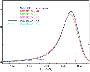
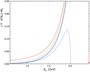
The effect of varying $J$ is shown in Fig. 2. As expected, variations in the peak region as a function of $J$ are small, while variations in the tail are rather significant. In particular, as shown in the plot on the right, the $J=0$ curve approaches a constant at small $x$, the $J=1$ one falls as $x^{1}$, etc. These are artifacts of the resummation. Such artifacts are absent for $J=3$ (or larger) where the power fall-off is determined by the perturbative expansion itself, Eq. (17). Obviously, the natural choice in our case is $J=3$: singularities at $N=-3$ do appear in the perturbative expansion, so they should be allowed in the resummed spectrum. We will use the $J=3$ spectrum as the default choice below.

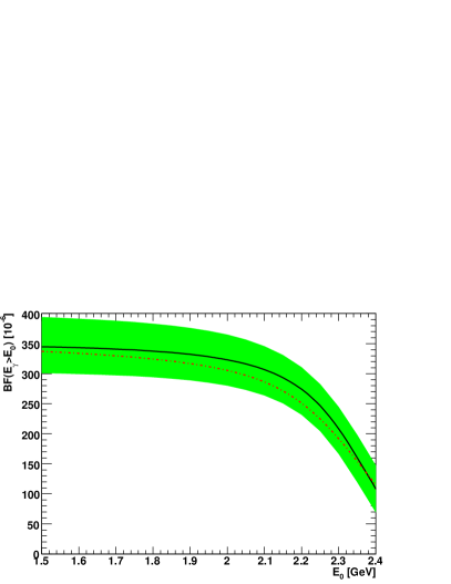
Having set the final resummation and matching formulae, let us examine the prediction for the partial BF as a function of the cut. The result is shown in Fig. 3. The figure compares the results obtained at NLO and at NNLO. Note that the Sudakov factor, which is computed as a Principal Value Borel sum, is the same (formally it has NNLL accuracy) — only the matching coefficient (A.3) is truncated at different orders. The error is significantly reduced at small $E_{0}$ cuts, where the corrections in the matching coefficient are essential.

2.3 All–order results in the large–$\beta_{0}$ limit 

Running–coupling effects often constitute a major part of the radiative corrections in QCD [62, 63, 64]. The typical situation is that the average gluon virtuality is lower, sometimes quite significantly lower, than the hard scale in the process, $m$. Thus, when the latter is used as the default renormalization scale for coupling ($\mu=m$), one encounters large corrections involving powers of $(\beta_{0}\alpha_{s}(m)/\pi)$, to any order in perturbation theory. In simple cases perturbative predictions can therefore be significantly improved by using the BLM scale instead. Differential spectra involve other parametrically–large corrections, such as Sudakov logarithms. Since they inherently depend on several scales, a straightforward scale–setting procedure is excluded. In such cases resummation is necessary.

In case of the $b\to X_{s}\gamma$ spectrum ${\cal O}(C_{F}\beta_{0}{\alpha_{s}}^{2})$ running–coupling (BLM) corrections have been computed long ago [65]. When using $\mu=m_{b}$, these corrections are very significant. A couple of years ago running–coupling terms in the $G_{77}$ spectrum, $C_{F}\beta_{0}^{n-1}{\alpha_{s}}^{n}$, were computed to all orders [18, 29]. Recently, the full ${\cal O}({\alpha_{s}}^{2})$ calculation of $G_{77}$ was performed [39, 42], finding that the additional, non-BLM corrections are, instead, moderate. Figs. 4 and 1 present these results for the normalized differential $b\to X_{s}\gamma$ spectrum.

Figure 4: Convergence of the perturbative expansion in Eq. (23), generated by running–coupling effects only, for the $O_{7}$ decay spectrum: partial sums of order ${\cal O}({\alpha_{s}}^{n})$ with $n=1$ through 4 are shown together with the Borel sum of Eq. (19). Left: the whole range of energies on a logarithmic vertical axis. Right: a restricted range on a linear scale. In both plots the horizontal axis ends at $E_{\gamma}=m_{b}/2$, as dictated by the support of these functions. The $\delta(E_{\gamma}-m_{b}/2)$ is not shown. In the plot on the right hand side the additional full lines at NNLO and beyond include the full ${\cal O}({\alpha_{s}}^{2})$ corrections based on the calculation of Ref. [39], see Eq. (2.3) and (2.3) below.

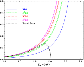
The plots clearly show that the $C_{F}\beta_{0}^{n-1}{\alpha_{s}}^{n}$ corrections are very large. In particular, if the expansion is performed in terms of $\alpha_{s}(m_{b})$, the ${\cal O}(C_{F}\beta_{0}{\alpha_{s}}^{2})$ term completely dominate the ${\cal O}({\alpha_{s}}^{2})$ correction. This is true even at fairly large $E_{\gamma}$, despite the presence of formally leading Sudakov logarithms with other color factors. With this numerical evidence it is easy to reach the conclusion that Sudakov resummation is not needed, or cannot significantly improve the description of the spectrum (see e.g. the discussion in Ref. [29]). The purpose of this section is to demonstrate that this conclusion is wrong, and that multiple soft and collinear gluon emission does in fact play an important rôle in shaping the spectrum through higher–order corrections. To this end we compare the fixed–order results with (1) DGE, where Sudakov logarithms are taken into account through exponentiation in moment space; and (2) the single–dressed–gluon (SDG) approximation, which accounts for real–emission running–coupling $C_{F}\beta_{0}^{n-1}{\alpha_{s}}^{n}$ corrections, to all orders, but neglects Sudakov logarithms. We will show that while the SDG series is Borel–summable for $E_{\gamma}\mathrel{\mathchoice{\vbox{\offinterlineskip\halign{$\m@th\displaystyle\hfil#\hfil$\cr<\crcr\sim\crcr} }}{\vbox{\offinterlineskip\halign{$\m@th\textstyle\hfil#\hfil$\cr<\crcr\sim\crcr} }}{\vbox{\offinterlineskip\halign{$\m@th\scriptstyle\hfil#\hfil$\cr<\crcr\sim\crcr} }}{\vbox{\offinterlineskip\halign{$\m@th\scriptscriptstyle\hfil#\hfil$\cr<\crcr\sim\crcr} }}}2$ GeV, it does not provide a viable description of the spectrum anywhere in the peak region, in sharp contrast with the DGE result.

The single–dressed–gluon approximation

The all–order calculation of the $G_{77}$ decay spectrum in the large–$\beta_{0}$ limit was performed in Ref. [18]. Using the scheme–invariant Borel transform with $\Lambda$ defined in the ${\overline{\rm MS}}$ scheme the result takes the form:

$$\frac{1}{\Gamma_{O_{7}}}\frac{d\Gamma_{O_{7}}}{dx} = \delta(1-x)+\left[\frac{C_{F}}{2\beta_{0}}\int_{0}^{\infty}du\,T(u)\,\left(\frac{\Lambda^{2}}{m_{b}^{2}}\right)^{u}\,B(x,u)\right]_{+}$$ (19)

with $m_{b}$ the bottom pole mass,

$$\beta_{0}=\frac{11}{12}N_{c}-\frac{1}{6}N_{f}$$ (20)

and

$$B(x,u) \equiv {\rm e}^{\frac{5}{3}u}\,\frac{\sin\pi u}{\pi u}\,x^{3}\,(1-x)^{-u}\int_{0}^{1}d\alpha\,\alpha\,(1-\alpha)^{-u}\,\times$$

$$\bigg{[}\frac{1}{(1-x\alpha)^{2}}\left(1-4\alpha+\alpha^{2}-\frac{(1-\alpha)^{2}}{1-u}\right)+\frac{1-\alpha}{(1-x\alpha)(1-u)}+\frac{2}{1-x}\frac{1}{1-x\alpha}+\frac{1}{1-x}\bigg{]}$$

$$= {\rm e}^{\frac{5}{3}u}\,\frac{\sin\pi u}{\pi u}\,x^{3}\,(1-x)^{-u}\Bigg{\{}\frac{1}{1-x}\frac{1}{(1-u)(2-u)}+$$

$$\left[-\frac{(1-4x+x^{2})}{x^{3}}\left(\frac{1}{1-x}+\frac{1}{1-u}\right)+\frac{2(1-x)^{2}}{(1-u)^{2}x^{3}}\right]\,\,_{2}F_{1}\Big{(}[1,1],[2-u],x\Big{)}$$

$$+\frac{(1-4x+x^{2})}{x^{3}}\frac{1}{1-x}+\frac{(x+1)(x^{2}-3x+1)}{(1-u)x^{3}(1-x)}-\frac{(2-x)}{(2-u)x^{2}}-\frac{2(1-x)}{(1-u)^{2}x^{3}}\Bigg{\}}.$$

In Ref. [18] the Borel function was expressed as an integral over a single Feynman parameter (the first expression above). Here we performed this integral and wrote the Borel function in terms of a hypergeometric function.

Strictly within the large–$\beta_{0}$ limit $T(u)=1$. It is straightforward to take into account running–coupling effects beyond this level by an appropriate choice of the function $T(u)$ in the Borel integral. To account for $\beta_{1}$ terms to all orders it is sufficient to use the $T(u)$ of Eq. (2.1), see Ref. [51]. This will be done in the perturbative expansion, Eq. (23), and in the numerical analysis that follows.

Let us now examine the result of Eq. (2.3). The first observation is that this Borel function has no renormalon singularities. To see this note first that (despite appearance) there is no double pole at $u=1$ inside the curly brackets: for $u\longrightarrow 1$ the hypergeometric function reduces to ${}_{2}F_{1}\Big{(}[1,1],[2-u],x\Big{)}\longrightarrow 1/(1-x)$, so the double pole cancels. Now, since the curly brackets contain just simple poles at integer values of $u$, upon taking the $\sin\pi u$ factor into account, one concludes that there in no renormalon in $B(x,u)$.

The absence of Borel singularities may be interpreted as an indication that the perturbative expansion in $x$ space should be good. As we shall see this is not the case. First of all, at large $x$ the effective scales are parametrically lower than $m_{b}$ [18]: the dynamics is dominated by momenta of order $m_{b}\sqrt{1-x}$, the jet mass, and $m_{b}(1-x)$, the soft scale associated with the momentum distribution of the b quark. The analytic expression in (2.3) immediately indicates the presence of the former through its $(1-x)^{-u}$ dependence; to isolate the latter it is convenient to first apply the identity:

$$_{2}F_{1}\Big{(}[1,1],[2-u],x\Big{)}=(1-u)\left[-\frac{1}{u}\,_{2}F_{1}\Big{(}[1,1],[1+u],1-x\Big{)}+\frac{\pi}{\sin\pi u}(1-x)^{-u}x^{u-1}\right]$$ (22)

in (2.3), revealing the dependence on $(1-x)^{-2u}$. Moreover, the absence of renormalons does not imply the existence of the Borel sum: the Borel integral (19) may not converge at $u\to\infty$. It turns out that the Borel integral exists for sufficiently small $x$ values, but it does not exist at large $x$. We shall return to discuss this issue below, after considering the perturbative expansion order by order.

As usual, renormalons do appear upon taking moments [18]: when integrating over all values of $x$, including the endpoint region $x\to 1$, soft gluons necessarily contribute and consequently, infrared renormalon singularities at integer and half integer values of $u$ are generated. We emphasize that this is not a disadvantage of the moment space formulation, but rather its strength: renormalon singularities are a useful tool to understand the rôle of non-perturbative power corrections.

Perturbative expansion in $x$ space in the large–$\beta_{0}$ limit

The perturbative expansion of Eq. (19) is:

$$\frac{1}{\Gamma_{O_{7}}}\frac{d\Gamma_{O_{7}}}{dx}=\delta(1-x)+\frac{C_{F}}{\beta_{0}}\,\sum_{n=1}^{\infty}a_{n}\,\left[r^{\beta_{0}}_{n}(x)\right]_{+}\times\Big{(}1+{\cal O}(1/\beta_{0})\Big{)},$$ (23)

where

$$a_{n} \equiv\frac{1}{n!}\int_{0}^{\infty}du\,T(u)\,\left(\frac{\Lambda^{2}}{m_{b}^{2}}\right)^{u}\,u^{n}=\left(-\frac{d}{d\ln m_{b}^{2}}\right)^{n}\left(\frac{\alpha_{s}(m_{b})\beta_{0}}{\pi}\right)=\left(\frac{\alpha_{s}(m_{b})\beta_{0}}{\pi}\right)^{n}+\cdots,$$ (24)

where the dots stand for higher–order terms, ${\cal O}({\alpha_{s}}^{n+1})$ and so on, containing powers of $\beta_{1}/\beta_{0}^{2}$. Up to ${\cal O}({\alpha_{s}}^{2})$ such terms do not appear, and Eq. (23) reduces to

$$\frac{1}{\Gamma_{O_{7}}}\frac{d\Gamma_{O_{7}}}{dx}=\delta(1-x)+\frac{\alpha_{s}(m_{b})}{\pi}C_{F}\left[r^{\beta_{0}}_{1}(x)\right]_{+}+\left(\frac{\alpha_{s}(m_{b})}{\pi}\right)^{2}C_{F}\beta_{0}\left[r^{\beta_{0}}_{2}(x)\right]_{+}+\cdots.$$ (25)

The coefficients $r^{\beta_{0}}_{n}$ can be obtained order by order from the expansion of $\frac{1}{2}B(x,u)=\sum_{n=0}^{\infty}r^{\beta_{0}}_{n}(x)\,u^{n}/n!$ in Eq. (2.3). To this end we need the expansion of the hypergeometric function, which is available based on Ref. [66]. We present this expansion and the resulting coefficients up to ${\cal O}({\alpha_{s}}^{4})$ in Appendix B.

It is straightforward to include the remaining $C_{F}^{2}$ and $C_{A}C_{F}$ terms at ${\cal O}({\alpha_{s}}^{2})$ based on the results of Ref. [39]:

$$\frac{1}{\Gamma_{O_{7}}}\frac{d\Gamma_{O_{7}}}{dx} = \delta(1-x)+\frac{\alpha_{s}(m_{b})}{\pi}C_{F}\left[r_{1}(x)\right]_{+}$$

$$+ C_{F}\left[N_{f}r_{2}^{N_{f}}(x)+C_{F}r_{2}^{C_{F}}(x)+C_{A}r_{2}^{C_{A}}(x)\right]_{+}\left(\frac{\alpha_{s}(m_{b})}{\pi}\right)^{2}+\cdots$$

$$= \delta(1-x)+\frac{\alpha_{s}(m_{b})}{\pi}C_{F}\left[r^{\beta_{0}}_{1}(x)\right]_{+}$$

$$+ C_{F}\left[\beta_{0}r^{\beta_{0}}_{2}(x)+C_{F}r_{2}^{C_{F}}(x)+C_{A}\left(r_{2}^{C_{A}}(x)+\frac{11}{2}r_{2}^{N_{f}}(x)\right)\right]_{+}\left(\frac{\alpha_{s}(m_{b})}{\pi}\right)^{2}+\cdots.$$

The partial sums of Eq. (23) as well as the Borel sum of Eq. (19) include the large–$\beta_{0}$, $r^{\beta_{0}}_{n}(x)$ terms at each order. Thus, to have a complete result to ${\cal O}({\alpha_{s}}^{2})$ we now include the non-BLM ($C_{F}$ and $C_{A}$) terms in the square brackets of Eq. (2.3). When using Borel summation for the running–coupling contributions the normalized spectrum at NNLO can be expressed as:

$$\frac{1}{\Gamma_{O_{7}}}\frac{d\Gamma_{O_{7}}}{dx} = \delta(1-x)+\left[\frac{C_{F}}{2\beta_{0}}\int_{0}^{\infty}du\,T(u)\,\left(\frac{\Lambda^{2}}{m_{b}^{2}}\right)^{u}\,B(x,u)\right]_{+}$$

$$+ C_{F}\left[C_{F}r_{2}^{C_{F}}(x)+C_{A}\left(r_{2}^{C_{A}}(x)+\frac{11}{2}r_{2}^{N_{f}}(x)\right)\right]_{+}\left(\frac{\alpha_{s}(m_{b})}{\pi}\right)^{2}+\cdots.$$

The results are shown together with the pure running–coupling contributions in the plot on the right hand side in Fig. 4. As already concluded in Ref. [39], these additional contributions are moderate, so at least at this order, the running–coupling contributions dominate.

Let us now examine the convergence of the expansion and the possibility to sum up the series à la Borel. Fig. 4 summarizes the numerical results using $m_{b}=4.875$ GeV and $\Lambda=0.332$ GeV with $N_{f}=4$ and two–loop running coupling. The partial sums obtained by truncation of Eq. (23) at increasing orders converge well at small energies $E_{\gamma}\mathrel{\mathchoice{\vbox{\offinterlineskip\halign{$\m@th\displaystyle\hfil#\hfil$\cr<\crcr\sim\crcr} }}{\vbox{\offinterlineskip\halign{$\m@th\textstyle\hfil#\hfil$\cr<\crcr\sim\crcr} }}{\vbox{\offinterlineskip\halign{$\m@th\scriptstyle\hfil#\hfil$\cr<\crcr\sim\crcr} }}{\vbox{\offinterlineskip\halign{$\m@th\scriptscriptstyle\hfil#\hfil$\cr<\crcr\sim\crcr} }}}1.5$ GeV and less so as the energy increases. Nevertheless, the increasing–order contributions do decrease monotonically. This decrease is related of course to the absence of renormalons in Eq. (2.3). This usually means that the series is Borel summable. However, since it is a divergent series there is no straightforward relation between partial sums and the Borel sum.

As anticipated, the series is in fact Borel summable only below a certain energy, $x<x_{\max}$: the convergence of the Borel integral at large $u$ is guaranteed only owing to the suppression by $(\Lambda^{2}/m_{b}^{2})^{u}$; as already observed in Ref. [18], because of the presence of $(1-x)^{-2u}$ contributions in $B(x,u)$ (see Eq. (22)), it is predominantly the soft scale $m_{b}(1-x)$ which sets the argument of the coupling at large $x$. Based on these considerations we can deduce from Eq. (2.3) an estimate of where the Borel sum will cease to exist:

$$E_{\gamma}^{\max}\simeq\frac{m_{b}}{2}\left(1-{\rm e}^{5/6}\Lambda/m_{b}\right)\simeq 2.06\,\,{\rm GeV}.$$ (28)

Indeed, as shown in Fig. 4 the Borel sum is close to the high–order partial sums at small energies and to lower–order ones at higher energies, until it eventually reaches a peak, bends downwards and becomes negative. Soon after it breaks down completely owing to non-convergence of the $u$ integral at $u\longrightarrow\infty$, in accordance with Eq. (28).

We note that increasing–order partial sums become quite different from each other at $E_{\gamma}\mathrel{\mathchoice{\vbox{\offinterlineskip\halign{$\m@th\displaystyle\hfil#\hfil$\cr>\crcr\sim\crcr} }}{\vbox{\offinterlineskip\halign{$\m@th\textstyle\hfil#\hfil$\cr>\crcr\sim\crcr} }}{\vbox{\offinterlineskip\halign{$\m@th\scriptstyle\hfil#\hfil$\cr>\crcr\sim\crcr} }}{\vbox{\offinterlineskip\halign{$\m@th\scriptscriptstyle\hfil#\hfil$\cr>\crcr\sim\crcr} }}}2$ GeV; this obviously means they cannot be thought of as an approximation to the spectrum. Also the corresponding Borel sum, although unique where it exists, does not look anything like a physical spectrum would. Its complete breakdown according to (28) is indicative of the low scales involved. But even if the bottom mass were much higher, this SDG approximation cannot be expected to describe the Sudakov region. Running–coupling corrections are not the most important corrections for $E_{\gamma}\longrightarrow m_{b}/2$. In the large–$\beta_{0}$ limit the most singular terms at large $x$ are ${\alpha_{s}}^{n}\,C_{F}\,{\beta_{0}}^{n-1}\ln^{n}(1-x)/(1-x)$, while the full perturbative expansion contains double logarithms of form ${\alpha_{s}}^{n}\,{C_{F}}^{n}\,\ln^{2n-1}(1-x)/(1-x)$, as well as other subleading logarithms which are associated with multiple soft and collinear emission. With increasing order, the latter become more important at large $x$ compared to the former. Finally, returning to Fig. 1, we observe the remarkable difference between increasing–order partial sums and the DGE result in the peak region. The gap between them should be understood as the contribution of multiple soft and collinear gluon emission, with a particular regularization of the divergent sum. In contrast with the fixed–order partial sums and the SDG Borel sum, the DGE result provides a useful approximation to the spectrum in the peak region.

3 Resummed spectra for individual matrix elements other than $G_{77}$ 

In Sec. 2 we considered in some detail the calculation of the normalized spectrum of the magnetic dipole operator. It is well known that in contrast with the total width, the spectrum is not so sensitive to the details of the short–distance interaction, and therefore the $G_{77}$ spectrum computed above can be thought of as an approximation to the physical spectrum. However, to make precision estimates of the partial BF as a function of the cut, it is important to compute the spectra of other matrix elements as well. Since fixed–order results for all matrix elements but $G_{77}$ are available to ${\cal O}(\alpha_{s})$ only, the accuracy we can hope to achieve in the description of the spectra of individual $G_{ij}$ matrix elements is not as high.

We will make the approximation where the matrix elements $G_{ij}$ (for any $i$ and $j$ other than 77) are written as ${\cal O}(\alpha_{s})$ hard coefficient functions, which are ${\cal O}(N^{0})$ for $G_{i7}$ interference terms and ${\cal O}(N^{-1})$ for other terms, times the same Sudakov factor discussed in the context of $G_{77}$. This approximation is motivated by the following observations:

• Independently of the nature of the short–distance interaction, all non–integrable real–emission corrections at any order, namely corrections to the moments that scale as $N^{0}$ times logarithms at large $N$, are necessarily associated with soft and collinear radiation around the same Born–level configuration involving a b quark in the initial state and an unresolved quark jet in the final state.

• All operators mix into $O_{7}$ under renormalization. Moreover, the ${\cal O}(\alpha_{s})$ result of $G_{ij}$ is dominated by the virtual diagrams, which are proportional to the tree level $G_{77}$. This observation was already used in Ref. [49] arguing that ${\cal O}(N_{f}\alpha_{s}^{2})$ corrections can be well approximated by computing both real and virtual diagrams for $O_{7}$ and only virtual diagrams for $O_{1,2,8}$.

It should be noted that while the ${\cal O}(N^{0})$ interference terms do indeed involve the same Sudakov factor, ${\cal O}(N^{-1})$ contributions associated with integrable bremsstrahlung corrections, do not share this property, and in general involve a new jet function. In this respect, our calculation of the resummed spectra of $G_{ij}$ that do not involve $O_{7}$ is a cruder approximation; as we shall see the relative weight of these contributions, especially in the Sudakov region, is small.

The structure of this section is as follows: in Sec. 3.1 we discuss the small $E_{\gamma}$ behavior of the different matrix elements and then extend the matching procedure of Sec. 2 accordingly, using the known ${\cal O}(\alpha_{s})$ coefficients. In Sec. 3.2 we present numerical results for the resummed spectra of individual matrix elements, based on this ${\cal O}(\alpha_{s})$ matching procedure.

3.1 The small $E_{\gamma}$ asymptotic behavior and matching at ${\cal O}(\alpha_{s})$ 

Looking at the small photon–energy limit, $E_{\gamma}\to 0$, we find the following asymptotic behavior:

$$\frac{dG_{ij}(E_{0},m_{b})}{dE_{0}}={\cal O}(E_{0}^{3});$$ (29)

$${\mathrm{except}}\,\,{\mathrm{for}}\qquad\left\{\begin{array}[]{l}{\displaystyle\frac{dG_{88}(E_{0},m_{b})}{dE_{0}}=\frac{1}{E_{0}}}\left[C_{F}\frac{\alpha_{s}}{\pi}\frac{2}{9}\left(1-\ln\frac{m_{b}}{m_{s}}\right)\,+\,{\cal O}({\alpha_{s}}^{2})\right];\\ \\ {\displaystyle\frac{dG_{78}(E_{0},m_{b})}{dE_{0}}=\frac{4E_{0}}{m_{b}^{2}}}\left[C_{F}\frac{\alpha_{s}}{\pi}\frac{1}{3}\,+\,{\cal O}({\alpha_{s}}^{2})\right].\end{array}\right.$$

As discussed in Sec. 2.2, the phase–space suppression for $E_{\gamma}\to 0$ is $E_{\gamma}dE_{\gamma}$, and any additional suppression or enhancement of the $G_{ij}$ spectrum in this limit depends on the dynamics, and therefore on the operators $O_{i}$ and $O_{j}$. To understand the difference between $O_{8}$ and $O_{7}$ in this respect, note that in the $O_{8}$ amplitude the gluon couples to the flavor–changing current through $G^{\mu\nu}$ while the photon is emitted as bremsstrahlung, whereas in the $O_{7}$ case it is the other way around. While the $O_{7}$ coupling (4) gives rise to a linear dynamical suppression with the photon energy, photon bremsstrahlung involves a soft singularity, namely a $1/E_{\gamma}$ enhancement. Combining this behavior of the amplitudes with the phase–space factor one immediately obtains the different $E_{\gamma}\to 0$ limits in (29) for $G_{77}$, $G_{88}$ and the interference $G_{78}$. At ${\cal O}(\alpha_{s})$, the behavior of matrix elements containing $O_{1,2}$ is similar to that of $O_{7}$. The reason for this is that the photon cannot be emitted as bremsstrahlung, but must instead couple to the virtual charm propagating in the loop (the diagram with just gluon coupling to the charm loop vanishes).

Thus in most cases there is a cubic power suppression of the spectrum for extremely soft photons, $E_{\gamma}\to 0$. When matching Sudakov resummation for the high photon energy endpoint ($E_{\gamma}=m_{b}/2$) into the fixed–order results, it is therefore useful to take $J=3$ as for the $O_{7}$ contribution. As explained in detail in Sec. 2.2, in this way artifacts of resummation away from the hard photon endpoint are avoided (the more pronounced soft–energy tail of $O_{8}$ and its interference with $O_{7}$ will be accounted for at fixed order).

In general, the matching involves a separation of the real–emission contributions between momentum and moment space (see Sec. 3 and Appendix C in Ref. [17]). The separation we use is defined such that the leading contributions at small $\Delta$ are always treated in moment space:

$$\phi_{ij}(\Delta)=\tilde{\eta}_{ij}(\Delta)+\tilde{\xi}_{ij}(\Delta)\quad{\mathrm{with}}\quad\tilde{\xi}_{ij}(\Delta)=O(\Delta^{2}).$$ (32)

Introducing the Mellin transform of $\tilde{\eta}_{ij}(\Delta)$ as in [17]:

$$\tilde{\mu}_{ij}(N)\equiv\int_{0}^{1}dx\,x^{N-1}\left.\frac{d\tilde{\eta}_{ij}(\Delta)}{d\Delta}\right|_{\Delta=1-x};\qquad\tilde{\eta}_{ij}(\Delta)=\int_{c-i\infty}^{c+i\infty}\frac{dN}{2\pi\,i}\,\frac{(1-\Delta)^{1-N}}{N-1}\,\tilde{\mu}_{ij}(N),$$ (33)

we get:

$$G_{ij}(E_{\min},m_{b}) = C_{F}\frac{\alpha_{s}(m_{b})}{\pi}\left[\frac{3}{8}\delta_{j=7}{\rm Re}\left\{r_{i}+\gamma_{i7}^{(0)}\ln\frac{m_{b}}{\mu}\right\}+{\tilde{\eta}}_{ij}(\Delta)\right]$$ (34)

$$+\,C_{F}\frac{\alpha_{s}(m_{b})}{\pi}{\tilde{\xi}}_{ij}(\Delta)+{\cal O}({\alpha_{s}}^{2})$$

$$=\int_{c-i\infty}^{c+i\infty}\frac{dN}{2\pi\,i}\,\frac{(1-\Delta)^{1-N}}{N-1}\left[C_{F}\frac{\alpha_{s}(m_{b})}{\pi}V_{ij}^{(1)}(N)+{\cal O}({\alpha_{s}}^{2})\right]\times\widetilde{\rm Sud}^{(J)}(N,m_{b})$$

$$+\,C_{F}\frac{\alpha_{s}(m_{b})}{\pi}{\tilde{\xi}}_{ij}(\Delta)+{\cal O}({\alpha_{s}}^{2}),$$

where in the second expression used Eq. (33), included the Sudakov factor resumming large logarithms at ${\cal O}({\alpha_{s}}^{2})$ and beyond, and defined

$$V_{ij}^{(1)}(N)\equiv\frac{3}{8}\delta_{j=7}{\rm Re}\left\{r_{i}+\gamma_{i7}^{(0)}\ln\frac{m_{b}}{\mu}\right\}+{\tilde{\mu}}_{ij}(N).$$ (35)

Note that $\tilde{\mu}_{ij}(N)$ are all ${\cal O}(1/N)$ (Appendix C in [17]) so $V_{ij}^{(1)}(N)$ is of ${\cal O}(1)$ at large $N$ for $j=7$ (the interference terms for any $i$ are ${\cal O}(1)$ at large $N$) while it is ${\cal O}(1/N)$ otherwise.

For $77$, $78$ and $88$ matrix elements the NLO contribution is treated entirely in moment space: $\tilde{\eta}_{ij}(\Delta)=\tilde{\phi}_{ij}(\Delta)$ and $\tilde{\xi}_{ij}(\Delta)=0$, so

$$\tilde{\mu}_{78}(N) = \frac{2}{3}\left[-\frac{1}{(N-1)N}(\Psi(N)+\gamma_{E})+\frac{1}{N^{2}}+\frac{1}{4}\frac{1}{N+2}+\frac{1}{N}\right].$$ (36)

and

$$\tilde{\mu}_{88}(N) = -\left[\frac{2}{9}\frac{1}{N}-\frac{2}{9}\frac{1}{N-1}-\frac{1}{9}\frac{1}{N+1}\right]\left(\ln\frac{m_{b}}{m_{s}}-\frac{1}{2}\Psi(N)-\frac{1}{2}\gamma_{E}\right)$$

$$-\frac{1}{18}\frac{1}{N+2}+\frac{1}{6}\frac{1}{N}-\frac{2}{9}\frac{1}{N-1}+\frac{1}{36}\frac{1}{N+1}+\frac{1}{9N^{2}}-\frac{1}{18}\frac{1}{(1+N)^{2}}.$$

Note that the latter expression has a pole at $N=1$, owing to the soft–photon singularity. However, this should not affect the calculation of $G_{ij}(E_{\min},m_{b})$ with non-zero $E_{\min}$ so long as the contour in Eq. (34) is to the right of $N=1$.

For all the other contributions, namely the ones associated with the operators $O_{1}$ and $O_{2}$ and their interference with $O_{7}$ and $O_{8}$ (this includes $\phi_{22}$, $\phi_{27}$, $\phi_{11}$, $\phi_{12}$ $\phi_{17}$, $\phi_{18}$ and $\phi_{28}$) we introduce a separation according to Eq. (32) with a non-trivial $\tilde{\xi}_{ij}(\Delta)$. The specific separation used in Appendix C in [17] was based on defining $\tilde{\eta}_{ij}(\Delta)$ as the leading–order term in the expansion of $\phi_{ij}(\Delta)$ at small $\Delta$. This simple procedure is not adopted here, since it would introduce a constant differential spectrum at very small $E_{\gamma}$, in contradiction with the power suppressed behavior of Eq. (29). Instead we will define $\tilde{\eta}_{ij}(\Delta)$ such that it would capture both the small $\Delta$ limit and certain features of the $\Delta\to 1$ limit. As shown in Appendix C in [17] for small $\Delta$, ${\phi}_{ij}(\Delta)$ is ${\cal O}(\Delta)$, so according to Eq. (32) we require

$$\mathrm{for}\,\,\mathrm{small}\,\,\Delta:\hskip 110.0pt\tilde{\eta}_{ij}(\Delta)\simeq{\phi}_{ij}^{\prime}(\Delta=0)\times\Delta+{\cal O}(\Delta^{2}).$$ (38)

As explained above (see Eq. (29)) for $\Delta\to 1$ the differential spectrum falls as the third power $1-\Delta$ so the integrated spectrum approaches a constant as the fourth power of $(1-\Delta)$. We therefore require:

$$\mathrm{for}\,\,\mathrm{large}\,\,\Delta:\hskip 90.0pt\tilde{\eta}_{ij}(\Delta)\simeq{\phi}_{ij}(\Delta=1)+{\cal O}\Big{(}(1-\Delta)^{J+1}\Big{)},$$ (39)

where $J=3$, such that $(1-\Delta)^{4}$ contributions appear through both the moment–space expression ($\tilde{\eta}_{ij}$) and the momentum–space residual ($\tilde{\xi}_{ij}$), while ones with $(1-\Delta)^{h}$ for $h=1,2,3$, which are absent in the physical spectrum, do not appear in either. Both ${\phi}_{ij}^{\prime}(\Delta=0)$ and ${\phi}_{ij}(\Delta=1)$ can be explicitly computed from the expressions in Eq. (C.1) in [17]. To accommodate (38) and (39) we define:

$$\tilde{\eta}_{ij}(\Delta)\equiv\phi_{ij}(\Delta=1)\bigg{[}1-(1-\Delta)^{J+1}\,\Big{(}1+(J+1)\Delta\Big{)}\bigg{]}+\phi^{\prime}_{ij}(\Delta=0)\,(1-\Delta)^{J+1}\,\Delta.$$ (40)

In computing $G_{ij}(E_{0},m_{b})/G_{ij}(E_{\min},m_{b})$ using Eq. (34), $\tilde{\xi}_{ij}(\Delta)$ is readily obtained using $\tilde{\xi}_{ij}(\Delta)=\phi_{ij}(\Delta)-\tilde{\eta}_{ij}(\Delta)$, while $\tilde{\mu}_{ij}(N)$ is computed according to Eq. (33) by the Mellin conjugate of the derivative of Eq. (40), namely:

$$\tilde{\mu}_{ij}(N) \equiv\int_{0}^{1}d\Delta\,(1-\Delta)^{N+J-1}\Big{[}\phi_{ij}(\Delta=1)\,(J+1)(J+2)\Delta\,+\,\phi^{\prime}_{ij}(\Delta=0)\,\big{(}1-(J+2)\Delta\big{)}\Big{]}$$

$$=\frac{(J+1)(J+2)}{(N+J)(N+J+1)}\phi_{ij}(\Delta=1)+\frac{N-1}{(N+J)(N+J+1)}\phi^{\prime}_{ij}(\Delta=0).$$ (41)

As required, the first moment $\tilde{\mu}_{ij}(N=1)$, corresponding to the total width, is given by $\phi_{ij}(\Delta=1)$, while the large–$N$ asymptotic behavior is determined by $\phi^{\prime}_{ij}(\Delta=0)$. Importantly, when using the matching procedure of Eq. (34), where $\widetilde{\rm Sud}^{(J)}(N,m_{b})$ is given by Eq. (18) and $\tilde{\mu}_{ij}(N)$ by Eq. (3.1), we are guaranteed that no spurious singularities at $N>-J$ would appear (singularities do appear for $N=-J$, $N=-J-1$ etc.), which could alter the small–$E_{\gamma}$ behavior.

3.2 Resummed spectra for individual matrix elements 

In the previous sections we established a procedure for matching the Sudakov–resummed spectrum with the known fixed–order expansion. For $G_{77}$ this is done to NNLO, ${\cal O}({\alpha_{s}}^{2})$, while for the matrix elements of other operators and their interference with $O_{7}$, to ${\cal O}(\alpha_{s})$. This allows us to study the shape of each contribution and eventually have better control on the cut dependence of the total BF.

Figure 5: Left: the contribution to the spectrum from the separate operators and their mixing, together with their sum, the total width, based on Eq. 4.1. We notice that the dominant contributions (from 77 and 27) have similar shapes in the Sudakov region, although their tails for small $E_{\gamma}$ are significantly different. Right: the spectrum of each matrix element $\Gamma_{ij}$ (see Eq. (4.1)) has been normalised to better display the various shapes. Since effectively $O_{1}=\frac{1}{6}O_{2}$, the curves for 17 and 27 are identical. The same is true for the groups (18, 28) and (11, 12, 22).

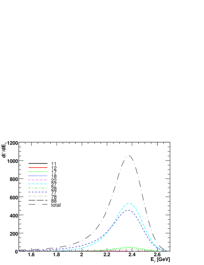
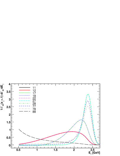
Figure 5 shows the contributions to the differential BF from each matrix element $G_{ij}$ according to Eq. 4.1 below, as well as a comparison between the shapes (normalized spectra) of the different matrix elements. In general, it confirms the lore that the shapes of the spectra of the most contributing operators do not vary much, and the shape of the total spectrum is roughly the same as the one for $O_{7}$. However, the shapes are not completely identical and the details do depend on the relative contributions of the different operators. These depend of course also on the coefficient functions. Numerically, the most important effect in the experimentally accessible energy range is that of $G_{27}$ which is comparable in magnitude to $G_{77}$, but is somewhat narrower. The effect it has on the differential distribution along the tail, e.g. between $1.8$ and $2$ GeV, is significant. The $G_{78}$ spectrum, on the other hand, is somewhat wider and it has a higher small-$x$ tail. A rather different, and significantly wider shape is presented by $G_{28}$ and even wider still by $G_{22}$ (and likewise those corresponding to $O_{1}$ instead of $O_{2}$). These affect the differential spectrum at smaller energies, below $1.8$ GeV.

4 Partially–integrated BF and moments with a photon–energy cut

In the previous sections we computed the ${\bar{B}}\longrightarrow X_{s}\gamma$ spectra using DGE. We improved the calculation in Ref. [17] in various ways: we included the NNLO corrections in full in the $G_{77}$ sector (Sec. 2.1 and Appendix A), introduced a new method to constrain the behavior of the resummed spectrum away from the Sudakov region (Sec. 2.2 and Appendix A.3), and matched the resummed spectrum with the fixed–order expansion, separately for each matrix element $G_{ij}$ (Sec. 3). In this section we will make use of these advancements to make predictions for measurable quantities: the partial BF and the first few moments as a function of the cut on the photon energy. We begin in Sec. 4.1 by computing the total BF and discussing its theoretical uncertainty, then in Sec. 4.2, we consider the partial BF with a cut and discuss cut–dependent uncertainties, and finally in Sec. 4.3 we present results for the first few moments and analyze numerically the relation between renormalon contributions, power corrections and support properties.

4.1 The total BF

The calculation of the total BF presents a challenge in its own [7, 8]. First, this calculation has to accommodate a large hierarchy of scales $M_{W},m_{t}\gg m_{b}$. This is dealt with [4, 5, 6, 7, 8] by the well–established machinery of the effective Weak Hamiltonian, which facilitates the resummation of large logarithms, $\ln m_{W}/m_{b}$, to all orders in the strong coupling. Estimating the BF therefore involves the perturbative calculation of the matching coefficients at the high scales, evolution of the different operators from $M_{W}$ to $m_{b}$ and finally, the contribution of the matrix elements of the different operators to ${\bar{B}}\longrightarrow X_{s}\gamma$. The main challenge here is at the perturbative level: even the matrix elements present little sensitivity to non-perturbative effects.

The NLO calculation was completed 5 years ago (see [8] and Refs. therein) and some of the ingredients have been recently brought to the NNLO level. This includes, in particular, the matching coefficients at the Weak scale [46], partial calculation of the evolution matrix [47, 48] and, most importantly, the two–loop matrix element of the $O_{7}$ operator [44, 45]. However, other essential ingredients are still missing. Amongst these are the matrix elements of other operators, especially $G_{27}$, which contributes to the BF almost as much as $G_{77}$, despite the fact that its perturbative expansion starts at ${\cal O}(\alpha_{s})$, rather than at ${\cal O}(1)$. The renormalization scale of $G_{ij}$ other than $G_{77}$ is obviously not fixed at this level.

Beyond $G_{77}$, which is known to NNLO in full [44, 45], the virtual $\beta_{0}{\alpha_{s}}^{2}$ corrections to $G_{ij}$ have been computed in Ref. [49]. It is likely that these running–coupling corrections constitute a major part of the NNLO contribution — this has been supported by the finding of Ref. [44]. Here we shall make use of this available, partial NNLO information on the matrix elements, which are the most important ingredient, neglecting NNLO effects in the Wilson coefficients at the $M_{W}$ scale and in the evolution. A more complete NNLO BF estimate is due when some of the missing ingredients — in particular $G_{27}$ at ${\cal O}({\alpha_{s}}^{2})$ — become available.

Another difficulty in the evaluation of the BF is its sensitivity to the bottom mass, which is raised to the fifth power in (1). Amongst these five powers, two are associated with the operator itself, and therefore correspond to the short–distance mass $m_{b}^{\hbox{\tiny${\overline{\rm MS}}$}}$, whereas the additional three result from phase–space integration, and therefore correspond to the pole mass, $m_{b}$. As discussed in the introduction, the pole mass has a leading renormalon ambiguity at $u=1/2$, implying that the perturbative expansion of the total width in the on-shell scheme is badly divergent. Writing (1) order by order,

$$\Gamma(\bar{B}\longrightarrow X_{s}\gamma,E>E_{0}) = \frac{\alpha_{\rm em}G_{F}^{2}}{32\pi^{4}}\left|V_{\rm tb}V_{\rm ts}^{*}\right|^{2}\,\left(m_{b}^{\hbox{\tiny${\overline{\rm MS}}$}}(m_{b})\right)^{2}\,m_{b}^{3}\,$$

$$\hskip 60.0pt\times\,\sum_{i,j,\,i\leq j}C^{\hbox{\tiny eff}}_{i}(\mu)C_{j}^{\hbox{\tiny eff}}(\mu)\,{G_{ij}(E_{0},\mu)},$$

$$= \frac{\alpha_{\rm em}G_{F}^{2}}{32\pi^{4}}\left|V_{\rm tb}V_{\rm ts}^{*}\right|^{2}\,\left(m_{b}^{\hbox{\tiny${\overline{\rm MS}}$}}(m_{b})\right)^{2}\,m_{b}^{3}\,$$

$$\hskip 60.0pt\times\,\underbrace{\bigg{[}f_{0}(\mu)+f_{1}(\mu)\frac{\alpha_{s}(\mu)}{\pi}+f_{2}(\mu)\left(\frac{\alpha_{s}(\mu)}{\pi}\right)^{2}+\cdots\bigg{]}}_{F},$$

the expansion coefficients $f_{n}(\mu)$ are therefore expected to grow factorially with the order $n$ owing to running–coupling corrections. Judging from what we know of the pole mass — see Appendix B in Ref. [17] — this divergence sets in already at the first few orders. A similar situation occurs for other inclusive decays, for example for the charmless semileptonic decay ${\bar{B}}\longrightarrow X_{u}l\bar{\nu}$ [34, 35, 36]:

$$\Gamma_{\hbox{\tiny total}}\left({\bar{B}}\longrightarrow X_{u}l\bar{\nu}\right)=\frac{G_{F}^{2}|V_{\rm ub}|^{2}m_{b}^{5}}{192\pi^{3}}\underbrace{\bigg{[}1+s_{1}\frac{\alpha_{s}(\mu)}{\pi}+s_{2}(\mu)\left(\frac{\alpha_{s}(\mu)}{\pi}\right)^{2}+\cdots\bigg{]}}_{G_{u}}.$$ (43)

In this case the coefficients have been computed to NNLO in Ref. [70], where large running–coupling corrections already appear. Moreover, in this case it is possible to interpolate reliably [52] (see also Ref. [71, 72, 73]) between the first few orders and the known asymptotic behavior of the series, which is set by the $u=1/2$ renormalon of the pole mass. In this way a precise evaluation of the total charmless semileptonic BF can be made directly using the on-shell scheme, where the $u=1/2$ renormalon ambiguities of the pole mass and the series in $G_{u}$ in Eq. (43) are regularized using the PV prescription. According to Sec. 2 in Ref. [52], this results in the following values:

$$\left.m_{b}\right|_{\hbox{\tiny PV}}=4.89\,\pm 0.05\,{\rm GeV}\qquad\qquad\left.G_{u}^{1/5}\right|_{\hbox{\tiny PV}}=0.928\,\pm 0.002,$$ (44)

corresponding to $N_{f}=4$. Here the error in the pole mass $m_{b}$ is dominated by the error on the short distance mass $m_{b}^{\hbox{\tiny${\overline{\rm MS}}$}}=4.20\pm 0.04$ (as quoted in Table 1). The uncertainty in $\Gamma_{\hbox{\tiny total}}\left({\bar{B}}\longrightarrow X_{u}l\bar{\nu}\right)/|V_{\rm ub}|^{2}$ is largely determined by this error.

$G_{F}=1.16637\cdot 10^{-5}$ GeV-2;  $\alpha_{\rm em}=1/(130.3\pm 2.3)$

$|V_{\rm ts}|=(41.13\pm 0.63)\cdot 10^{-3}$; $|V_{\rm tb}|=0.999119\pm 0.000026$ [67]

$M_{W}=80.388\pm 0.035$ GeV

$m_{t}^{\hbox{\tiny${\overline{\rm MS}}$}}(m_{t}^{\hbox{\tiny${\overline{\rm MS}}$}})=165\pm 5$ GeV

$\alpha_{s}(M_{Z}=91.19)=0.1176\pm 0.0020$  $\Longrightarrow$  $\eta\equiv\alpha_{s}(M_{W})/\alpha_{s}(\mu)\simeq 0.561$

$m_{s}^{\hbox{\tiny${\overline{\rm MS}}$}}\simeq 0.15$ GeV

$m_{c}^{\hbox{\tiny${\overline{\rm MS}}$}}(m_{c}^{\hbox{\tiny${\overline{\rm MS}}$}})=1.295\pm 0.015$ GeV [68]

$m_{b}^{\hbox{\tiny${\overline{\rm MS}}$}}(m_{b}^{\hbox{\tiny${\overline{\rm MS}}$}})=4.20\pm 0.04$ GeV [68, 69]

Table 1: Values of input parameters in the calculation of the BF and their uncertainties.

A useful tool in the calculation of the total ${\bar{B}}\longrightarrow X_{s}\gamma$ width is to normalize it by the semileptonic width; both $b\to c$ and $b\to u$ have been used in the past. In this way one exploits the better control one has on higher–order corrections in the semileptonic case, and reduces the sensitivity to the pole mass. There is however an important difference between the radiative decay width (4.1) and the semileptonic one (43) in the power of the pole mass. Thus, while the ratio

$$\left.\Gamma(\bar{B}\longrightarrow X_{s}\gamma,E>E_{0})\right/\Gamma_{\hbox{\tiny total}}\left({\bar{B}}\longrightarrow X_{u}l\bar{\nu}\right)$$ (45)

itself is an observable, and therefore renormalon free, it still contains an explicit dependence on the pole mass through $(m_{\hbox{\tiny${\overline{\rm MS}}$}}/m_{b}^{\rm pole})^{2}$. This has been dealt with in the past by resorting to some alternative renormalon–free mass scheme, a step that unavoidably introduces some uncertainty that is hard to quantify. Here we suggest an alternative procedure that utilizes the charmless semileptonic width to eliminate the explicit power dependence on the pole mass and yet does not require any additional mass scheme. This procedure is explained below.

Using the semileptonic width

In order to use the semileptonic result (43) to normalize the radiative one (4.1) in a renormalon free manner, we first write the series for $F$ over $G_{u}^{3/5}$. By virtue of the cancallation of renormalon ambiguities in Eq. (4.1) and in Eq. (43), this ratio is renormalon free, so it can be evaluated at fixed order. To recover the result for the radiative decay width in Eq. (4.1) we then multiply the series for $F/G_{u}^{3/5}$ by the PV result [52] for $G_{u}$ quoted in Eq. (44), namely $G_{u}^{3/5}=(0.928)^{3/5}$ and use the corresponding PV pole mass in the overall $m_{b}^{3}$ power (the product $m_{b}^{3}G_{u}^{3/5}$ is prescription–independent, see Eq. (43)):

$$\begin{split}\Gamma(\bar{B}\longrightarrow X_{s}\gamma,E>E_{\min})&=\frac{\alpha_{\rm em}G_{F}^{2}}{32\pi^{4}}\left|V_{\rm tb}V_{\rm ts}^{*}\right|^{2}\,\left(m_{b}^{\hbox{\tiny${\overline{\rm MS}}$}}(m_{b})\right)^{2}\,\times\\ &\hskip 70.0pt\,m_{b}^{3}\,G_{u}^{3/5}\bigg{[}F(E_{\min})/G_{u}^{3/5}\bigg{]}_{\rm Fixed\,\,Order}\end{split}$$ (46)

with

$$\bigg{[}F(E_{\min})/G_{u}^{3/5}\bigg{]}_{\rm Fixed\,\,Order} \equiv f_{0}(\mu)+\left(f_{1}(\mu)-\frac{3}{5}s_{1}f_{0}(\mu)\right)\frac{\alpha_{s}(\mu)}{\pi}$$

$$+\left(f_{2}(\mu)-\frac{3}{5}s_{1}f_{1}(\mu)-\frac{3}{5}s_{2}(\mu)f_{0}(\mu)+\frac{12}{25}s_{1}^{2}\,f_{0}(\mu)\right)\left(\frac{\alpha_{s}(\mu)}{\pi}\right)^{2}+\cdots.$$

Similarly, in order to use the resummed calculation of the normalized integrated spectra for individual matrix elements, namely ${G_{ij}(E_{0})}/{G_{ij}(E_{\min})}$, we define

$$F_{ij}(E_{\min}) = C^{\hbox{\tiny eff}}_{i}(\mu)C_{j}^{\hbox{\tiny eff}}(\mu)\,{G_{ij}(E_{\min},\mu)}$$

$$= f_{0}^{ij}(\mu)+f_{1}^{ij}(\mu)\frac{\alpha_{s}(\mu)}{\pi}+f_{2}^{ij}(\mu)\left(\frac{\alpha_{s}(\mu)}{\pi}\right)^{2}+\cdots$$

and write

$$\Gamma(\bar{B}\longrightarrow X_{s}\gamma,E>E_{0}) = \frac{\alpha_{\rm em}G_{F}^{2}}{32\pi^{4}}\left|V_{\rm tb}V_{\rm ts}^{*}\right|^{2}\,\left(m_{b}^{\hbox{\tiny${\overline{\rm MS}}$}}(m_{b})\right)^{2}\,m_{b}^{3}\,$$

$$\times\,\sum_{i,j,\,i\leq j}G_{u}^{3/5}\bigg{[}F_{ij}(E_{\min})/G_{u}^{3/5}\bigg{]}_{\rm Fixed\,\,Order}\left[\frac{G_{ij}(E_{0})}{G_{ij}(E_{\min})}\right]_{\rm Resummed}.$$

This formula will be used for the numerical analysis that follows. In Fig. 5 above we show the contribution from each of the terms $\Gamma_{ij}$. Eq. (4.1) will allow us to study the theoretical uncertainties associated with different ingredients as a function of the cut.

The total BF and the theoretical uncertainty

Using Eq. (46) we obtain the following result for the total BF:

$${\rm BF}(E_{\gamma}>m_{b}/20)=\Big{(}357\,\,\pm 40_{(\mu)}\,\pm 19_{(\mu_{c})}\,\pm{21}_{({\rm param.})}\Big{)}\,\cdot 10^{-6},$$ (50)

where, as explained above, we used (4.1) to NNLO where $f_{1}(\mu)$ is the full NLO coefficient while $f_{2}(\mu)$ is the $\beta_{0}$ part of the NNLO corrections to the matrix elements, with the parameters of Table 1, which yield (44). The central value is based on $\mu=m_{b}$ and $\mu_{c}=m_{b}/2$, and the three errors represent the variation of (1) $\mu$ and (2) $\mu_{c}$ as explained below, and (3) the parametric uncertainty in $m_{b}^{\hbox{\tiny${\overline{\rm MS}}$}}$ and ${\alpha_{s}}^{\hbox{\tiny${\overline{\rm MS}}$}}$ according to Table 1, respectively.

Let us discuss now the theoretical uncertainty in some more detail. Having separated the calculation into that of Wilson coefficients on the one hand, and matrix elements on the other, the stability of the result with respect to the renormalization point of the operators becomes an essential measure of the accuracy of the calculation. It should be emphasized that by modifying $\mu$ in (4.1) or in (4.1) both the renormalization scale of the coupling and the factorization scale (i.e. the separation between the coefficient functions and the matrix elements) is changed. This necessarily implies reshuffling of contributions between different matrix elements according to the anomalous dimension matrix.

It should be noted that there are various possibilities for choosing the renormalization point of the short distance mass in (4.1), which are of course reflected in the anomalous dimension matrix. We have chosen to fix this scale at the pole mass $m_{b}$, rather than to vary it with $\mu$.

Figure 6: The scale dependence of the total BF (the BF with $E_{\gamma}>m_{b}/20$) at LO, NLO and NNLO, according to Eqs. (46) and (4.1). At NNLO only $\beta_{0}{\alpha_{s}}^{2}$ terms are included in $f_{2}(\mu)$.

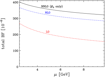
Figure 6 presents the variation of the total BF as a function of $\mu$, with the default parameters of Table 1 and with $\sqrt{z}\equiv m_{c}(\mu_{c})/m_{b}=0.2215$ (see below). We see that at leading order there is a large scale dependence (that of $(C_{7}^{\hbox{\tiny eff}}(\mu))^{2}$) which get significantly smaller at NLO and NNLO. Note that at NNLO only $\beta_{0}{\alpha_{s}}^{2}$ corrections are included here. The reason for suppressing the known ${\cal O}({\alpha_{s}}^{2})$ terms for $G_{77}$ beyond this approximation, is that there is a large cancellation, at each order in the expansion, between $G_{77}$ and $G_{27}$. It is therefore essential to include the same type of corrections for both. Note that there is no significant reduction of the scale dependence by including the $\beta_{0}{\alpha_{s}}^{2}$ NNLO corrections. This is a reflection of the fact that important NNLO corrections are still missing: the leading scale dependence at each order, ${\cal O}({\alpha_{s}}^{n}\ln^{n}m_{b}/\mu)$, is associated with the evolution of the operators and their mixing.

Another important source of uncertainty in the calculation of the total BF [7] is the renormalization point $\mu_{c}$ of the charm mass $m_{c}$ entering through the ratio $z\equiv m_{c}^{2}(\mu_{c})/m_{b}^{2}$ into the expressions for the matrix element involving $O_{2}$ (and $O_{1}$), notably $G_{27}$. We have chosen the central value for $z$ as $\sqrt{z}=0.2215$, corresponding to an intermediate renormalization point, $\mu_{c}\simeq m_{b}/2$ GeV, which is in between the b mass and the c mass. This is close to the central value chosen in [7]. For the error estimate we vary $z$ in the range suggested in that paper, namely $0.18\,<\,\sqrt{z}\,<\,0.26$. This uncertainty will reduce once the calculation of the matrix elements involving $O_{2}$ is complete.

Let us also note that the results of Ref. [49] for the $\beta_{0}{\alpha_{s}}^{2}$ corrections involving charm loops were computed as an expansion in $z=m_{c}(\mu_{c})/m_{b}$. When using this expansion we assume that it is valid at the physical value of $z$, an issue that was checked in Ref. [49]. Given that $z$ is already varied over a large range, we do not consider the residual error associate with using a finite–order expansion in $z$ as an independent source of uncertainty.

We note that the central value of Eq. (50) is somewhat lower than that of previous estimates. This is despite the fact that NNLO corrections increase the BF: using the same procedure at NLO we get ${\rm BF}(E_{\gamma}>m_{b}/20)=322\cdot 10^{-6}$. These results can be compared with the result by Gambino and Misiak [7]: ${\rm BF}(E_{\gamma}>m_{b}/20)=373\cdot 10^{-6}$, who used the NLO calculation. The main change is due to the different procedure for normalizing the BF by the semileptonic width. Note, in particular, that Ref. [7] evaluated the factor $m_{b}^{\hbox{\tiny${\overline{\rm MS}}$}}/m_{b}^{\rm pole}$ appearing in (45) by replacing it with $m_{b}^{\hbox{\tiny${\overline{\rm MS}}$}}/m_{b}^{1S}$. At NLO this replacement has no effect on the expansion since the expansion of $m_{b}^{1S}/m_{b}^{\rm pole}$ starts at ${\cal O}({\alpha_{s}}^{2})$, however, numerically, this ratio is $\sim 0.95$. This explains much of the difference in the central values between the two estimates. It should also be noted that the uncertainty we find from varying the renormalization scale $\mu$, $\pm 11\%$, is larger than those in Refs. [7, 8], and consequently the combined uncertainty on the total BF is about $\pm 13.7\%$, somewhat larger than previous estimates.

Finally, we point out that certain small corrections have been neglected in our calculation. The largest amongst these is the electroweak corrections whose effect has been estimated [7] to be $-3.8\%$ of the BF. Another correction is the power–suppressed $\Lambda^{2}/m_{b}^{2}$ that was estimated as $+2.5\%$ of the BF [7]. As soon as more complete NNLO results become available these corrections should be taken into account as well.

4.2 BF for $E_{\gamma}>E_{0}$

Figure 7: Left: The central value and uncertainty on the branching fraction ratio ${\rm BF}(E_{\gamma}>E_{0})$ as a function of the cut on the photon energy $E_{0}$. The black central line is obtained with the standard values of the parameters, while the (red) dot-dashed line is obtained by the same choice of parameters as for the dot-dashed line in Figs. 10 and 11. Right: The breakdown on sources to the uncertainty in the branching fraction.

In Fig. 7 we present the BF as a function of the cut, ${\rm BF}(E_{\gamma}>E_{0})$. The uncertainty band in this figure as well as in Figs. 3, 8 and 10 to 12, indicates the theoretical uncertainty obtained by varying separately the following parameters, and summing the respective uncertainties in quadrature:

• The renormalization scale of the operators (and the coupling) in the calculation of the total width according to Eqs. (46) and (4.1) between $m_{b}/2$ and $2m_{b}$ where $\mu=m_{b}$ is the default.

• The renormalization point $\mu_{c}$ of the charm mass $m_{c}(\mu_{c})$ entering the matrix elements involving $O_{2}$ and $O_{1}$. As mentioned above we use: $0.18\,m_{b}<\,m_{c}(\mu_{c})\,<\,0.26\,m_{b}$.

• The renormalization scale in the matching coefficients of the resummed spectra (A.3), between $m_{b}$ and $m_{b}/2$, where $\mu=m_{b}$ is the default.

• The parameters controlling the details of the quark distribution function (corresponding to the leading “shape function”) $B_{\cal S}(u)$, which enter the Sudakov factor in Eq. (18), with the corresponding power corrections, namely $(N\Lambda/m_{b})^{k}$ for any $k\geq 3$. Specifically, as discussed in Sec. 4.3 below, we vary $C_{3/2}$ in Eq. (13) (see Eqs. (3.27) to (3.29) in Ref. [52]) and $f^{\mathrm{PV}}$ in Eq. (53) below within a range that is determined based on the support properties of the spectra, according to $\mathrm{CutA,\,CutB}<0.01$, where the functions $\mathrm{CutA}$ and $\mathrm{CutB}$ are defined in (54).

• The short distance parameters, $\alpha_{s}^{\hbox{\tiny${\overline{\rm MS}}$}}$ and $m_{b}^{\hbox{\tiny${\overline{\rm MS}}$}}$, within their error ranges as indicated in Table 1.

Let us point out that the effect of the charm mass on the running of the coupling is neglected throughout the calculation of the spectra. We use $N_{f}=4$, and ignore the charm threshold. The consequences of this approximation have not yet been studied. They certainly worthwhile investigating since at large $N$ the coupling in the Sudakov factor is effectively evaluated at scales below the charm mass. We further neglect non-perturbative effects that go beyond the summation of the leading powers, $(N\Lambda/m_{b})^{k}$. This includes the so-called “subleading shape functions”, namely power corrections that are suppressed by $1/N$ compared to the ones we include, as well as the non-perturbative structure of the final state, which can be viewed as power corrections in $(N\Lambda^{2}/m_{b}^{2})$, or directly in momentum space as exclusive states.

Figure 8: Left: The central value and uncertainty on the branching fraction ratio ${\rm BF}(E_{\gamma}>E_{0})/{\rm BF}(E_{\gamma}>.2445\mathrm{GeV})$ and the branching fraction itself (insert) as a function of the cut on the photon energy $E_{0}$. Right: The breakdown on sources to the uncertainty in the branching fraction ratio. For low values of the cut, the uncertainty is dominated by the contribution from a variation in the renormalization scale in the matching coefficients (A.3). This relatively large effect is originating from the matrix elements other than $G_{77}$ that are known to NLO accuracy only. For $E_{0}\lesssim 2.1\,\mathrm{GeV}$, the parameters controlling the behavior in the Sudakov region contributes only little to the overall uncertainty. The (red) dot-dashed lines are obtained by the same choice of parameters as for the dot-dashed line in Figs. 10 and 11.

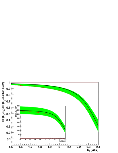
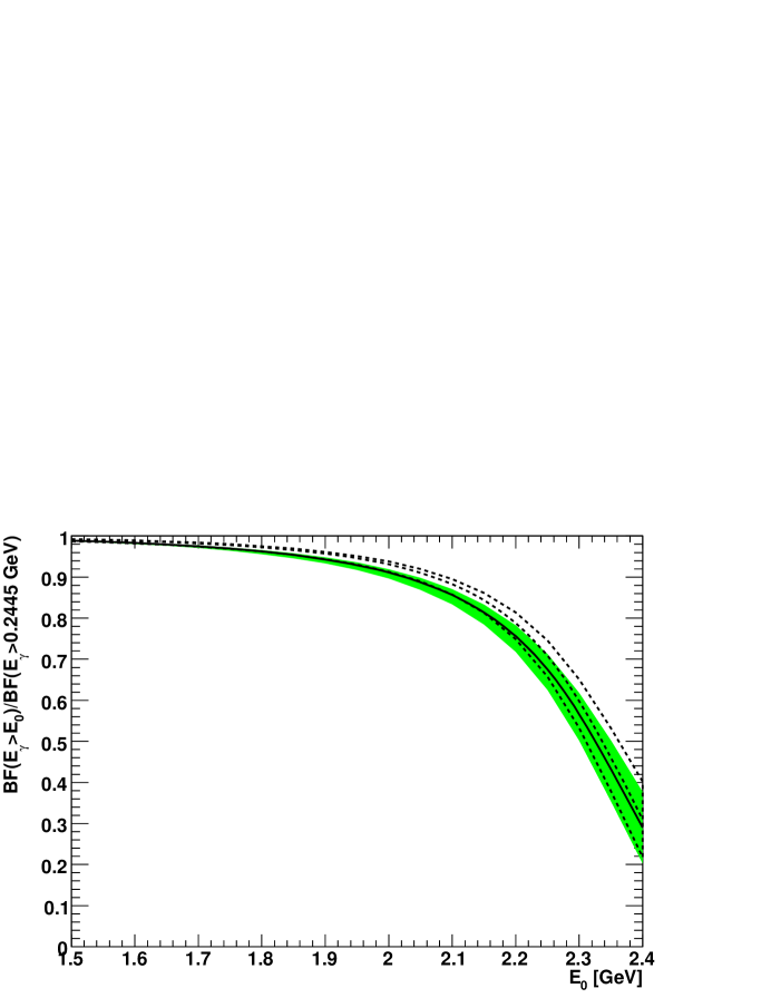
Excluding very high cut values, the largest uncertainties shown in Fig. 7 have very little dependence on the cut. This includes, in particular, the renormalization scale of the operators and the value of $m_{c}(\mu_{c})$. The cut dependence of these contributions, is entirely due to the change their variation induces on the relative weight of the different matrix elements in Eq. (4.1). Furthermore, Fig. 7 shows that the uncertainty associated with the values of the short distance parameters, is also insensitive to the cut for sufficiently mild cuts. It is therefore useful to analyze separately the cut–dependent uncertainty. This is done in Fig. 8, where we display the partial BF ratio ${\rm BF}(E_{\gamma}>E_{0})/{\rm BF}(E_{\gamma}>m_{b}/20)$ as a function of $E_{0}$. This ratio is needed, and can be used for extrapolating experimental measurements from the region $E_{\gamma}>E_{0}$ to the whole of phase space. Some numerical values for the extrapolation factor are presented in Table 2.

$E_{0}$ (GeV)	default	$\min$	$\max$
1.6	1.028	1.025	1.058
1.7	1.034	1.031	1.071
1.8	1.045	1.041	1.090
1.9	1.062	1.056	1.117
2.0	1.092	1.083	1.160
2.1	1.150	1.134	1.238
2.2	1.287	1.247	1.414
2.3	1.692	1.556	1.965

Table 2: Extrapolation factors for the ${\bar{B}}\longrightarrow X_{s}\gamma$ BF,   ${\rm BF}(E_{\gamma}>m_{b}/20)/{\rm BF}(E_{\gamma}>E_{0})$

As expected, the uncertainty of the extrapolation increases as the cut is increased. However, the rate of increase is not too high: precise experimental measurements with fairly stringent cuts, such as $E_{\gamma}>2.0$ GeV, can still be useful. As shown in Fig. 8, up to cuts as high as $E_{0}=2.3$ GeV, the largest source of uncertainty is still the dependence on the renormalization scale in the matching coefficients of Eq. (A.3). At higher cuts the $m_{b}$ dependence and the details of the quark distribution function, $B_{\cal S}(u)$ and the associated power corrections become dominant. For the higher moments of the photon energy these ingredients become important already at milder cuts. We therefore discuss these issues in more detail in the next section.

4.3 Spectral moments for $E_{\gamma}>E_{0}$

Figure 9: The region in the $u=3/2$ renormalon residue and power corrections plain, $(C_{3/2},f^{\mathrm{PV}})$, where the spectra conforms with the physical support properties. For example, in the most restricted region, marked by circles, both the requirement on the BF $\mathrm{CutA}(C_{3/2},f^{\mathrm{PV}})<0.01$ and the one on the average energy $\mathrm{CutB}(C_{3/2},f^{\mathrm{PV}})<0.01$ are satisfied ($\mathrm{CutA}$ and $\mathrm{CutB}$ are defined in Eq. (54)).

Figure 10: Left: The prediction for $M_{B}-\langle E_{\gamma}\rangle_{E_{\gamma}>E_{0}}$ as a function of $E_{0}$ compared with data from Belle and BaBar. The green band indicates the uncertainty, and is obtained by adding contributions in quadrature. The default choice of parameters, corresponding to $\mu=m_{b}^{\mathrm{PV}}$ in Eq. (A.3) and $(C_{3/2},f^{\mathrm{PV}})=(1,0)$ in Eqs. (13) and (53), is shown as a full (black) line. The dotted line is obtained by choosing $\mu=m_{b}^{\mathrm{PV}}/2$. A slightly better description of the data is obtained upon choosing $\mu=m_{b}^{\mathrm{PV}}/2$ and $(C_{3/2},f^{\mathrm{PV}})=(6.2,.3)$. This result is indicated by the (red) dot-dashed line. These choices all have equal theoretical justification. Right: The breakdown on sources for the uncertainty.

Spectral moments defined over a restricted energy range $E_{\gamma}>E_{0}$ [17], have proven to be a useful tool for comparison of the spectrum between experimental data and theory [14, 12, 13]. This comparison is important for a few reasons. First, it allows to test the extrapolation of ${\bar{B}}\longrightarrow X_{s}\gamma$ from the region of measurement. Second, more generally, it allows to test our understanding of the Sudakov region, which is a critical ingredient in extracting $|V_{\rm ub}|$ from semileptonic decays, ${\bar{B}}\longrightarrow X_{u}l{\bar{\nu}}$. It that case the extrapolation from the region of measurement into the whole of phase space is very large, a factor of $\sim 2-5$ depending on the specific kinematic cuts applied, and thus the sensitivity to the details of the spectrum in the peak region is significant.

Following Ref. [17] we consider here the average photon energy with a cut, namely

$$\left<E_{\gamma}\right>_{E_{\gamma}>E_{0}}\equiv\frac{\displaystyle\int_{E_{0}}dE_{\gamma}\,\frac{d\Gamma(E_{\gamma})}{dE_{\gamma}}\,E_{\gamma}}{\displaystyle\int_{E_{0}}dE_{\gamma}\,\frac{d\Gamma(E_{\gamma})}{dE_{\gamma}}}$$ (51)

and higher truncated moments, defined by:

$$\left<\left(\left<E_{\gamma}\right>_{E_{\gamma}>E_{0}}-E_{\gamma}\right)^{n}\right>_{E_{\gamma}>E_{0}}\equiv\frac{\displaystyle\int_{E_{0}}dE_{\gamma}\,\frac{d\Gamma(E_{\gamma})}{dE_{\gamma}}\,\left(\left<E_{\gamma}\right>_{E_{\gamma}>E_{0}}-E_{\gamma}\right)^{n}}{\displaystyle\int_{E_{0}}dE_{\gamma}\,\frac{d\Gamma(E_{\gamma})}{dE_{\gamma}}}.$$ (52)

It is obvious that the higher the cut, or the moment $n$ considered, the higher is the sensitivity to the fine details of the peak and, eventually, the endpoint region, $E_{\gamma}\simeq M_{B}/2$. In contrast to the BF with mild cuts, where one can obtain a purely perturbative prediction, when considering the moments or high cuts one must take account of power corrections. In DGE, this can be judged by the sensitivity of the Borel integral to values of $u$ away from the origin. In our parametrization of the soft function $B_{\cal S}(u)$ (see Eqs. (3.27) to (3.29) in Ref. [52]) this directly depends on $C_{3/2}$. Since $B_{\cal S}(u)$ at $u\mathrel{\mathchoice{\vbox{\offinterlineskip\halign{$\m@th\displaystyle\hfil#\hfil$\cr>\crcr\sim\crcr} }}{\vbox{\offinterlineskip\halign{$\m@th\textstyle\hfil#\hfil$\cr>\crcr\sim\crcr} }}{\vbox{\offinterlineskip\halign{$\m@th\scriptstyle\hfil#\hfil$\cr>\crcr\sim\crcr} }}{\vbox{\offinterlineskip\halign{$\m@th\scriptscriptstyle\hfil#\hfil$\cr>\crcr\sim\crcr} }}}3/2$ is not known, and since the significance of power corrections in (14) directly depends on what it is assumed to be, it becomes obvious that these two aspects must be addressed together, and that an additional constraint would be needed. Here we propose to use the support properties, namely the vanishing of the spectrum for $E_{\gamma}>M_{B}/2$ for this purpose.

In taking power corrections in the peak region into account one has to find a compromise that allows a sufficiently accurate description of the spectrum and yet involves a sufficiently small number of non-perturbative parameters. In general, starting with perturbation theory, the closer the region of interest to the endpoint, the harder it is to find such a compromise. Here we wish to explore the relation between $C_{3/2}$ in the parametrization of $B_{\cal S}(u)$ entering Eq. (18), the power corrections and the support properties. As a first exploration of this issue, it is reasonable to consider a single non-perturbative parameter. On the other hand, since we would like to explore extreme cuts — the support properties — there is no justification in using only the leading power term, $k=3$ in Eq. (14). For $E_{\gamma}\simeq M_{B}/2$ such hierarchy does not exist. In order to use Eq. (14) we therefore take a sum of all renormalon ambiguities, all weighted by one non-perturbative parameter, $f^{\hbox{\tiny PV}}$:

$$\begin{split}\left.\widetilde{\rm Sud}^{(J)}(N,m_{b})\right|_{\hbox{\tiny PV}}&\,\longrightarrow\,\left.\widetilde{\rm Sud}^{(J)}(N,m_{b})\right|_{\hbox{\tiny PV}}\times\\ &\exp\Bigg{\{}\frac{C_{F}}{\beta_{0}}\,\pi\,f^{\hbox{\tiny PV}}\,\sum_{k=3}^{\infty}\,\frac{T(k/2)}{k/2}\,\,B_{\cal S}(k/2)\left(\frac{\Lambda}{m_{b}}\right)^{k}\,R^{(J)}(N,k/2)\Bigg{\}},\end{split}$$ (53)

where $f^{\hbox{\tiny PV}}$ is expected to be of order $1$. Eq. (53) includes a sum of all powers of $(N\Lambda/m_{b})^{k}$ with $k\geq 3$, which a priori (depending on $B_{\cal S}(k/2)$) may all be relevant for $E_{\gamma}\simeq M_{B}/2$. Going over to milder cuts, where only the leading power is relevant, $f^{\hbox{\tiny PV}}$ can be identified with $f^{\hbox{\tiny PV}}_{3}$ in (14).

Figure 11: Left: The prediction for the second central moment $\left\langle\left(\langle E_{\gamma}\rangle_{E_{\gamma}>E_{0}}-E_{\gamma}\right)^{2}\right\rangle_{E_{\gamma}>E_{0}}$ as a function of $E_{0}$ compared with data from Belle and BaBar. The band indicating the uncertainty and the various lines are obtained with the same choice of parameters as the corresponding ones in Fig. 10. Right: The breakdown on sources for the uncertainty.

We already know from previous studies that very large values of $C_{3/2}$ or of power corrections cannot be accommodated with the support properties, $E_{\gamma}<M_{B}/2$. Here we would like to translate this into a concrete constraint. To this end we require that neither the spectrum nor the first moment extend too far beyond the physical endpoint. Considering all possible values of $C_{3/2}$ and $f^{\mathrm{PV}}$, we implement this requirement using the following cuts:

$$\begin{split}\mathrm{CutA}(C_{3/2},f^{\mathrm{PV}})&=\left|\frac{\Gamma(\bar{B}\longrightarrow X_{s}\gamma,E_{\gamma}>M_{B}/2)}{\Gamma(\bar{B}\longrightarrow X_{s}\gamma,E_{\gamma}>M_{B}/20)}\right|\\ \mathrm{CutB}(C_{3/2},f^{\mathrm{PV}})&=\left|1-\frac{\langle E_{\gamma}\rangle_{E_{\gamma}>M_{B}/2}}{M_{B}/2}\right|.\end{split}$$ (54)

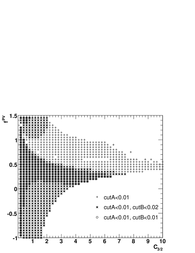
In Fig. 9 we have indicated by plus’s the region in the plane of $(C_{3/2},f^{\mathrm{PV}})$ for which the spectra conform to $\mathrm{CutA}(C_{3/2},f^{\mathrm{PV}})<0.01$ with the remaining parameters at their default value. We have also indicated by circles (asterisks) the region for which the spectra also obey $\mathrm{CutB}(C_{3/2},f^{\mathrm{PV}})\,<\,0.01\,(0.02)$.

We observe that there is a reasonably large range in the $(C_{3/2},f^{\mathrm{PV}})$ parameter space that conforms with the physical support properties. The details depend on how stringent the constrains on (54) are. What is general, however, is that acceptable spectra have power corrections that are typically of the order of the renormalon ambiguity: as shown in Fig. 9 $f^{\mathrm{PV}}\mathrel{\mathchoice{\vbox{\offinterlineskip\halign{$\m@th\displaystyle\hfil#\hfil$\cr<\crcr\sim\crcr} }}{\vbox{\offinterlineskip\halign{$\m@th\textstyle\hfil#\hfil$\cr<\crcr\sim\crcr} }}{\vbox{\offinterlineskip\halign{$\m@th\scriptstyle\hfil#\hfil$\cr<\crcr\sim\crcr} }}{\vbox{\offinterlineskip\halign{$\m@th\scriptscriptstyle\hfil#\hfil$\cr<\crcr\sim\crcr} }}}1$, except at very small $C_{3/2}$ where the power correction essentially has no effect.

Having excluded too large contributions to the Sudakov factor from large $u$ values and too large power corrections based on the support criterion, we still have a variety of spectra whose properties, i.e. the first few cut moments, are different. In the analysis of the theoretical uncertainty in this paper we allow $(C_{3/2},f^{\mathrm{PV}})$ to vary within the region of $\mathrm{CutA,\,CutB}<0.01$. It is reassuring that the power corrections satisfying these requirements are also of the order of the renormalon ambiguity, or smaller. Note, on the other hand, that for most of the range in $C_{3/2}$ vanishing power corrections are excluded as well.

Figure 12: Left: The prediction for the third central moment $\left\langle\left(\langle E_{\gamma}\rangle_{E_{\gamma}>E_{0}}-E_{\gamma}\right)^{3}\right\rangle_{E_{\gamma}>E_{0}}$ as a function of $E_{0}$. The band indicating the uncertainty and the various lines are obtained with the same choice of parameters as the corresponding ones in Fig. 10. Right: The breakdown on sources for the uncertainty. This plot is terminated when the prediction for the third moment becomes consistent with zero.

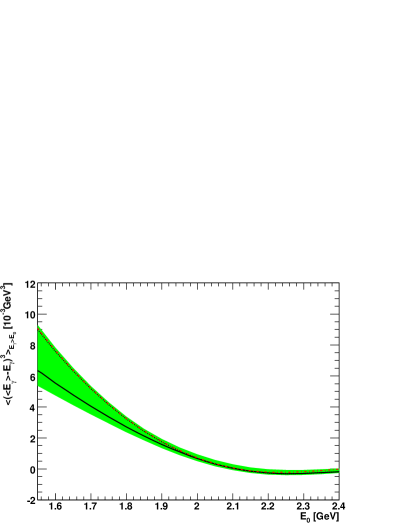
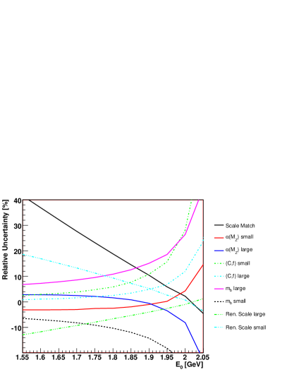
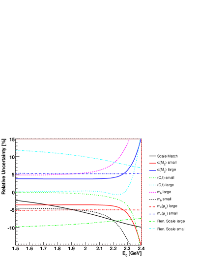
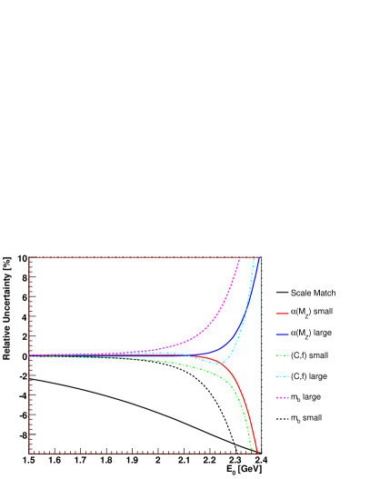
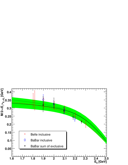
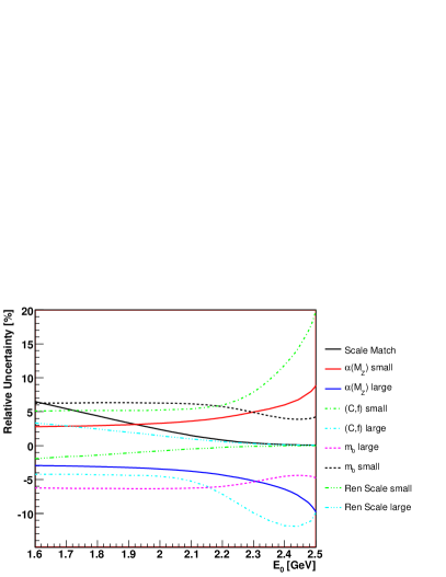
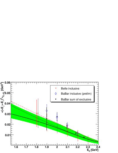
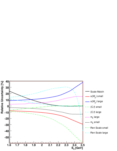
In Figs. 10 to 12 we show the cut dependence of the first three central moments, $M_{B}-\left<E_{\gamma}\right>_{E_{\gamma}>E_{0}}$ where the average energy is defined in (51), the variance $n=2$ in (52) and the third moment $n=3$ in (52), respectively. The bands in the figures on the left hand side represent the estimated theoretical uncertainty obtained by the same procedure used in Sec. 4.2. The various contributions to the uncertainty are presented in the plots on the right. As expected, the uncertainty associated with the behavior of the quark distribution function, $B_{\cal S}(u)$ at $u\sim 3/2$, and the corresponding power corrections increases as the cut is raised. It also gets more significant of course for higher moments.

In the average energy and variance figures, Figs. 10 and 11, we also present experimental data [14, 12, 13] by Belle and two analysis by BaBar. Fits to data, with simultaneous variation of $m_{b}$, $C_{3/2}$ and $f^{\hbox{\tiny PV}}$, can be very useful for the measurement of the bottom mass and for testing the theoretical description of the peak region. We do not perform any such fits here, and the comparison with data is merely qualitative.

The default line (full line) in Figs. 10 and 11, corresponding to the $C_{3/2}=1$ choice made in Refs. [17, 52] with no power corrections $f^{\hbox{\tiny PV}}=0$, seems to agree very well with the Belle data, and not as good with the BaBar data that often has smaller errors. In particular, in the average energy plot, the theoretical curve lies quite significantly above the BaBar data point at $E_{0}=2.26$ GeV; in the variance plot it is about two sigma below the BaBar data points at $E_{0}<2.1$ GeV. When making this comparison one should take great care in interpreting theoretical uncertainties, which do not reflect probability. For example, there is absolutely no theoretical preference to the choice $C_{3/2}=1$ with $f^{\hbox{\tiny PV}}=0$ as compared, for example to $C_{3/2}=6.2$ with $f^{\hbox{\tiny PV}}=0.3$. Similarly, there is no preference for choosing the renormalization scale in (A.3) as $\mu=m_{b}$ (our default) as compared to $\mu=m_{b}/2$. Short of further calculations, these choices remain arbitrary to a large extent. We note that with these different choices there is good agreement with BaBar data. This is demonstrated by the dot-dashed lines in Figs. 10 and 11.

5 Conclusions 

We presented here a calculation of the ${\bar{B}}\longrightarrow X_{s}\gamma$ branching fraction, as well as the first few spectral moments as a function of a cut on the photon energy, using the framework of Dressed Gluon Exponentiation. Building on our previous work [17, 52], and on recent progress in fixed–order calculations [44, 45, 39, 42, 49], we now have accurate predictions for these observables and good understanding of the theoretical uncertainties and their dependence on the cut.

We made progress on several different aspects of the calculation:

• In matching the resummed spectrum into the fixed–order expansion (Appendix A), we made full use of the available NNLO results of the $G_{77}$ spectrum [39, 42]. In this sector we therefore have a complete NNLO with NNLL accuracy. As shown in Fig. 1 the DGE spectrum does not vary much in going from NLO to NNLO, indicating that all important higher–order corrections are indeed resummed. The largest relative variation is along the tail of the distribution where NNLO corrections in the matching coefficient are important (see also Fig. 3).

• We developed a method to perform Sudakov resummation without violating the analytic structure of the perturbative series in moment space, and therefore, without generating artifacts away from the Sudakov region. Using the Sudakov factor (18) the resummed spectrum can therefore be used down to small $E_{\gamma}$ where it matches into the fixed–order result (See Fig. 2).

• Matrix elements of other operators in the effective Weak Hamiltonian and their interference with $O_{7}$ are known in full to ${\cal O}(\alpha_{s})$ only. However, we also know that independently of the nature of the short–distance interaction, all important contributions in the peak region, i.e. ones that do not vanish as ${\cal O}(1/N)$, necessarily involve the same Sudakov factor. Here we computed the spectra of individual matrix elements $G_{ij}$ assuming the same Sudakov factor multiplied by ${\cal O}(\alpha_{s})$ hard coefficient functions that depend on the operators. The resulting effect on the spectrum is shown in Fig. 5.

• We performed a first numerical study of the relation between renormalon contributions to the quark distribution function, power corrections, and support properties. To this end we used the parametrization of the soft anomalous dimension function $B_{\cal S}(u)$ proposed in Ref. [52] (see Eqs. (3.27) to (3.29) there), which is consistent with all available constraints for $u\to 0$, and at $u=1/2$ and $u=1$; it includes a single parameter $C_{3/2}$ that controls the $u\mathrel{\mathchoice{\vbox{\offinterlineskip\halign{$\m@th\displaystyle\hfil#\hfil$\cr>\crcr\sim\crcr} }}{\vbox{\offinterlineskip\halign{$\m@th\textstyle\hfil#\hfil$\cr>\crcr\sim\crcr} }}{\vbox{\offinterlineskip\halign{$\m@th\scriptstyle\hfil#\hfil$\cr>\crcr\sim\crcr} }}{\vbox{\offinterlineskip\halign{$\m@th\scriptscriptstyle\hfil#\hfil$\cr>\crcr\sim\crcr} }}}3/2$ region, which is not well constrained theoretically. We also used a simple formula with a single parameter for the corresponding power corrections, Eq. (53), which nevertheless takes into account all powers of $(N\Lambda/m_{b})^{k}$ with $k\geq 3$. Under these assumptions we showed that there exists a range in the parameter space where the computed spectrum conforms with the physical support properties. We observed that the size of the power corrections is of the order of the renormalon ambiguity, as expected on general grounds.

• We proposed a new method to evaluate the total ${\bar{B}}\longrightarrow X_{s}\gamma$ width that utilizes the semileptonic width, where the leading renormalon ambiguity has been explicitly dealt with using Borel summation [52]. Our new method avoids using any additional mass scheme. The result for the total BF is summarized in Eq. (50). It is consistent with previous determinations [7, 8]. Unfortunately, despite having partial NNLO information on the matrix elements [44, 45, 49], the theoretical uncertainty is still large, $\pm 13.7\%$. We observed large cancellations between $G_{77}$ and $G_{27}$ contributions, which vary depending on the renormalization scale. Therefore, significant improvement is expected upon completion of the NNLO calculation of $G_{27}$.

• Finally, we devised a method to compute the BF with a cut on the photon energy, by combining the resummed calculation of the spectrum of individual matrix elements with the proper weight, given by the fixed–order calculation of the total BF, Eq. (4.1). This framework facilitates the analysis of theoretical uncertainties associated with different ingredients, which are known at different orders, and have different rôle depending on how stringent the cut is.

It is of theoretical as well as practical interest to understand the behavior of higher–order corrections. The overwhelming dominance of running–coupling corrections at ${\cal O}({\alpha_{s}}^{2})$, and the very late settling of the leading logarithmic behavior at large $x$ [39], might be interpreted as a signal that Sudakov resummation is irrelevant. In order to address the relative significance of higher–order corrections of different origin we presented in Sec. 2.3 the all–order resummation of the $G_{77}$ spectrum in the large–$\beta_{0}$ limit, based on the calculation of Ref. [18]. When working directly in momentum space ($x$ space) there are no renormalon ambiguities in the real–emission result, but there are convergence constraints on the Borel integral. Consequently, the Borel sum does not exist for $E_{\gamma}\mathrel{\mathchoice{\vbox{\offinterlineskip\halign{$\m@th\displaystyle\hfil#\hfil$\cr>\crcr\sim\crcr} }}{\vbox{\offinterlineskip\halign{$\m@th\textstyle\hfil#\hfil$\cr>\crcr\sim\crcr} }}{\vbox{\offinterlineskip\halign{$\m@th\scriptstyle\hfil#\hfil$\cr>\crcr\sim\crcr} }}{\vbox{\offinterlineskip\halign{$\m@th\scriptscriptstyle\hfil#\hfil$\cr>\crcr\sim\crcr} }}}2$ GeV. As shown in Fig. 1 and 4, the large–$\beta_{0}$ sum does not give a viable description of the spectrum in the peak region. This stands in sharp contrast with DGE, which through real–virtual cancellation and exponentiation in moments space, accounts for multiple soft and collinear radiation. Thus, despite the late settling of the leading logarithmic behavior at large $x$ up to ${\cal O}({\alpha_{s}}^{2})$, such logarithms are important at higher orders. It is the combination of soft gluon resummation with the resummation of running–coupling corrections that open the way for the quantitative description of inclusive decay spectra.

Finally, the results of the present paper can help in various ways in understanding and using the B factory ${\bar{B}}\longrightarrow X_{s}\gamma$ data. In order to make comparison between the BF measurements with a given kinematic cut, $E_{\gamma}>E_{0}$, and the theoretical result of Eq. (50) we provided in Table 2 estimates of the extrapolation factor as a function of $E_{0}$. This information, as well as all other details of the spectrum and the moments computed here, can be obtained using a ${\tt c^{++}}$ program that is made publicly available. Beyond the issue of the BF itself, combining the theoretical calculations presented here with ${\bar{B}}\longrightarrow X_{s}\gamma$ data is extremely valuable for other aspects of flavor physics: it allows a precise determination of the the b–quark mass, as well as testing and improving the description of inclusive decay spectra in the Sudakov region by quantifying Fermi–motion corrections. This is particularly important for the determination of $|V_{\rm ub}|$ from the B factory measurements of charmless semileptonic decays[74, 15].

Note Added: Upon completion of this paper there appeared two new papers addressing the calculation of the total BF [75, 76]. In particular, Ref. [76] estimates the ${\cal O}(\alpha_{s}^{2})$ contribution of the four–quark operator matrix elements using extrapolation from large $m_{c}$. This goes beyond the large–$\beta_{0}$ results of Ref. [49] that we used here. The final result for the total BF in [75, 76] is consistent with ours, but has a lower central value and a significantly smaller uncertainty from varying the renormalization scale. The reasons for that are not yet clear.

Appendix A NNLO matching of the resummed $G_{77}$ spectrum

A.1 Expansion of the Sudakov exponent and a basic NNLO matching formula 

Let us begin by recalling the ${\cal O}({\alpha_{s}}^{2})$ result for the Sudakov exponent [17]. Expanding Eq. (2.1) to this order one obtains Eq. (9) with

$$E_{1}(N) = -\frac{a_{1}}{2}\bigg{(}S_{1}^{2}(N)-S_{2}(N)\bigg{)}-(b_{1}-d_{1})S_{1}(N)$$ (55)

$$E_{2}(N) = \bigg{[}-\frac{a_{1}}{2}S_{1}^{3}(N)+\left(d_{1}-\frac{1}{2}b_{1}-\frac{1}{2}a_{2}\right)S_{1}^{2}(N)+\left(d_{2}-b_{2}+\frac{3}{2}a_{1}\,S_{2}(N)\right)S_{1}(N)$$

$$+\left(-d_{1}+\frac{1}{2}b_{1}+\frac{1}{2}a_{2}\right)S_{2}(N)-\frac{1}{2}a_{1}\,S_{3}(N)\bigg{]}\beta_{0}$$

where we define

$$S_{k}(N)\equiv (-1)^{k-1}\,(k-1)!\sum_{l=1}^{N-1}\frac{1}{l^{k}}\,=\,\Psi_{k-1}(N)-\Psi_{k-1}(1),$$

$${\rm so} S_{1}(N)=\Psi(N)+\gamma_{E},\,\,\,S_{2}(N)=\Psi_{1}(N)-\frac{\pi^{2}}{6},$$

$$S_{3}(N)=\Psi_{2}(N)+2\zeta_{3},\,\,\,S_{4}(N)=\Psi_{3}(N)-\frac{\pi^{4}}{15}.$$

and where the coefficients of the Sudakov anomalous dimensions, defined in the $\overline{\rm MS}$ scheme, are [43, 53, 17, 39, 54, 55]:

$$\begin{split}a_{1}&=1,\qquad a_{2}=\frac{5}{3}+\left(\frac{1}{3}-\frac{1}{12}\pi^{2}\right)\frac{C_{A}}{\beta_{0}},\\ a_{3}&=-\frac{1}{3}+\frac{1}{\beta_{0}}\left[\left(\frac{55}{16}-3\zeta_{3}\right)C_{F}+\left(\frac{253}{72}-\frac{5}{18}\pi^{2}+\frac{7}{2}\zeta_{3}\right)C_{A}\right]\\ &+\frac{1}{\beta_{0}^{2}}\left[\left(-\frac{7}{18}-\frac{1}{18}\pi^{2}-\frac{11}{4}\zeta_{3}+\frac{11}{720}\pi^{4}\right)C_{A}^{2}+\left(-\frac{605}{192}+\frac{11}{4}\zeta_{3}\right)C_{A}C_{F}\right],\\ b_{1}&=-\frac{3}{4},\qquad b_{2}=-\frac{247}{72}+\frac{1}{6}\pi^{2}+\frac{1}{\beta_{0}}\left[\left(-\frac{3}{32}-\frac{3}{2}\zeta_{3}+\frac{1}{8}\pi^{2}\right)C_{F}+\left(-\frac{73}{144}+\frac{5}{2}\zeta_{3}\right)C_{A}\right],\\ d_{1}&=1,\qquad d_{2}=\frac{1}{9}+\frac{C_{A}}{\beta_{0}}\left[\frac{9}{4}\zeta_{3}-\frac{\pi^{2}}{12}-\frac{11}{18}\right].\end{split}$$ (57)

In the following we will compute the matching coefficient functions $H(\alpha_{s}(m_{b}),N)$ and $\Delta R(\alpha_{s}(m_{b}),x)$ in Eq. (8) to ${\cal O}({\alpha_{s}}^{2})$ based on the known NNLO expansion [39] and the expansion of the exponent in Eq. (9) with (55).

To this end we will need the color decomposition of the NNLO result in Eq. (5) (note that an overall factor of $C_{F}$ was extracted there). The NLO coefficients entering $R(\alpha_{s}(m_{b}),x)$ and $V(\alpha_{s}(m_{b}))$ are $r_{1}(x)$, which is is given explicitly Eq. (107) below, and $k_{1}=-31/12$. The NNLO ones will be decomposed as follows:

$$\begin{split}k_{2}&=N_{f}k_{2}^{N_{f}}+C_{F}k_{2}^{C_{F}}+C_{A}k_{2}^{C_{A}};\\ r_{2}^{\hbox{\tiny sing.}}(x)&=N_{f}r_{2}^{N_{f},\hbox{\tiny sing.}}(x)+C_{F}r_{2}^{CF,\hbox{\tiny sing.}}(x)+C_{A}r_{2}^{C_{A},\hbox{\tiny sing.}}(x);\\ r_{2}^{\hbox{\tiny reg.}}(x)&=N_{f}r_{2}^{N_{f},\hbox{\tiny reg.}}(x)+C_{F}r_{2}^{CF,\hbox{\tiny reg.}}(x)+C_{A}r_{2}^{C_{A},\hbox{\tiny reg.}}(x).\end{split}$$ (58)

The explicit expression for $r_{2}^{N_{f},\hbox{\tiny reg.}}(x)=-\frac{1}{6}r_{2}^{\beta_{0},\hbox{\tiny reg.}}(x)$ is given in Eq. (108) while the expressions for the other terms, corresponding to the $C_{F}^{2}$ and $C_{F}C_{A}$ color factors, can be found in Eqs. (7) and (8) in Ref. [39], respectively. Below we quote only their singular parts, $r_{2}^{\hbox{\tiny sing.}}(x)$, which were derived already in [17]. The regular parts, $r_{2}^{\hbox{\tiny reg.}}(x)$, are used here but owing to their length we do not write their explicit expressions here; these can read off Eqs. (7) and (8) in Ref. [39] by removing the $\delta$ and the plus–distribution terms. Using this color decomposition one finds the constants $k_{n}$ by integrating $r_{n}^{\hbox{\tiny reg.}}(x)$ according to Eq. (6) [39]:

$$k_{2}^{N_{f}}=\frac{49}{48}-\frac{\zeta_{3}}{3}+\frac{\pi^{2}}{16}=1.237;\qquad k_{2}^{C_{A}}=-4.795;\qquad k_{2}^{C_{F}}=1.216.$$ (59)

Having set the notation let us consider now the partially–integrated $G_{77}$ matrix element at ${\cal O}({\alpha_{s}}^{2})$, as obtained from Eq. (7) with (5):

$$\frac{G_{77}(E_{0},m_{b})}{G_{77}(0,m_{b})} = 1+C_{F}\left[k_{1}\frac{\alpha_{s}(m_{b})}{\pi}+k_{2}\left(\frac{\alpha_{s}(m_{b})}{\pi}\right)^{2}+\cdots\right]$$

$$+ C_{F}\int_{x_{0}=2E_{0}/m_{b}}^{1}\!\!\!\!\!dx\left[r_{1}^{\hbox{\tiny sing.}}(x)\frac{\alpha_{s}(m_{b})}{\pi}+r_{2}^{\hbox{\tiny sing.}}(x)\left(\frac{\alpha_{s}(m_{b})}{\pi}\right)^{2}+\cdots\right]_{+}$$

$$+ C_{F}\int_{x_{0}=2E_{0}/m_{b}}^{1}\!\!\!\!\!dx\bigg{(}r_{1}^{\hbox{\tiny reg.}}(x)\frac{\alpha_{s}(m_{b})}{\pi}+r_{2}^{\hbox{\tiny reg.}}(x)\left(\frac{\alpha_{s}(m_{b})}{\pi}\right)^{2}+\cdots\bigg{)}.$$

Defining the moments of $r_{n}^{\hbox{\tiny sing.}}(x)$ according to Eq. (2),

$$R_{n}^{\hbox{\tiny sing.}}(N)\equiv\int_{0}^{1}dx\,x^{N-1}\,\Big{[}r_{n}^{\hbox{\tiny sing.}}(x)\Big{]}_{+}=\int_{0}^{1}dx\left(x^{N-1}-1\right)r_{n}^{\hbox{\tiny sing.}}(x),$$ (61)

we find:

$$\int_{x_{0}=2E_{0}/m_{b}}^{1}\!\!\!\!\!dx\left[r_{n}^{\hbox{\tiny sing.}}(x)\right]_{+}=\frac{1}{2\pi i}\int_{c-i\infty}^{c+i\infty}\frac{dN}{N-1}\,\left(\frac{2E_{0}}{m_{b}}\right)^{1-N}\,R_{n}^{\hbox{\tiny sing.}}(N)$$ (62)

Thus, we can express Eq. (A.1) as an inverse–Mellin transform:

$$\frac{G_{77}(E_{0},m_{b})}{G_{77}(0,m_{b})} = \frac{1}{2\pi i}\int_{c-i\infty}^{c+i\infty}\frac{dN}{N-1}\!\left(\frac{2E_{0}}{m_{b}}\right)^{1-N}\!\!\Bigg{\{}1+C_{F}\bigg{[}k_{1}\frac{\alpha_{s}(m_{b})}{\pi}+\,k_{2}\left(\frac{\alpha_{s}(m_{b})}{\pi}\right)^{2}+\cdots\bigg{]}$$

$$+\,C_{F}\,\left[R_{1}^{\hbox{\tiny sing.}}(N)\frac{\alpha_{s}(m_{b})}{\pi}+R_{2}^{\hbox{\tiny sing.}}(N)\left(\frac{\alpha_{s}(m_{b})}{\pi}\right)^{2}+\cdots\right]\Bigg{\}}$$

$$+\,C_{F}\,\int_{x_{0}=2E_{0}/m_{b}}^{1}\!\!\!\!\!dx\bigg{(}r_{1}^{\hbox{\tiny reg.}}(x)\frac{\alpha_{s}(m_{b})}{\pi}+r_{2}^{\hbox{\tiny reg.}}(x)\left(\frac{\alpha_{s}(m_{b})}{\pi}\right)^{2}+\cdots\bigg{)}$$

Next, we can incorporate the resummation of Sudakov logarithms by rewriting Eq. (A.1) in terms of the Sudakov factor of Eq. (2.1) according to the general form in Eq. (8):

$$\left[\frac{G_{77}(E_{0},m_{b})}{G_{77}(0,m_{b})}\right]_{\rm Resummed}=\frac{1}{2\pi i}\int_{c-i\infty}^{c+i\infty}\frac{dN}{N-1}\,\left(\frac{2E_{0}}{m_{b}}\right)^{1-N}\,{\rm Sud}(N,m_{b})$$ (64)

$$\hskip 50.0pt\times\exp\left[C_{F}k_{1}\frac{\alpha_{s}(m_{b})}{\pi}+C_{F}\left(\bar{k}_{2}-C_{F}k_{1}^{2}/2\right)\left(\frac{\alpha_{s}(m_{b})}{\pi}\right)^{2}+\cdots\right]$$

$$\hskip 50.0pt+C_{F}\int_{x_{0}=2E_{0}/m_{b}}^{1}\!\!\!\!\!dx\bigg{(}r_{1}^{\hbox{\tiny reg.}}(x)\frac{\alpha_{s}(m_{b})}{\pi}+\bar{r}_{2}^{\hbox{\tiny reg.}}(x)\left(\frac{\alpha_{s}(m_{b})}{\pi}\right)^{2}+\cdots\bigg{)}.$$

Note that $\bar{r}_{2}^{\hbox{\tiny reg.}}(x)$ introduced here is different from $r_{2}^{\hbox{\tiny reg.}}(x)$ used in Eq. (A.1) since the exponentiation generates some additional integrable terms (see below). Such terms need to be subtracted of $r_{2}^{\hbox{\tiny reg.}}(x)$ to avoid double counting. Of course, $\bar{k}_{2}$ is defined accordingly, $\bar{k}_{n}\equiv-\int_{0}^{1}dx\,\bar{r}_{n}^{\hbox{\tiny reg.}}(x)$.

Upon expansion, this formula together with the coefficients of the Sudakov exponent was used to predict [17] the terms that diverge at $N\longrightarrow\infty$ at ${\cal O}(\alpha_{s}^{2})$, see Appendix A there. Explicit calculations later confirmed these results [39, 42]. Expanding Eq. (64) using Eq. (9) one gets, under the inverse–Mellin integral:

$$1+C_{F}\left[\left(R_{1}^{\hbox{\tiny sing.}}(N)+k_{1}\right)\frac{\alpha_{s}(m_{b})}{\pi}+\left(\bar{R}_{2}^{\hbox{\tiny sing.}}(N)+\bar{k}_{2}\right)\left(\frac{\alpha_{s}(m_{b})}{\pi}\right)^{2}+\cdots\right],$$ (65)

where

$$R_{1}^{\hbox{\tiny sing.}}(N)=E_{1}(N),\,\,\,\qquad\bar{R}_{2}^{\hbox{\tiny sing.}}(N)=\left(\frac{1}{2}E_{1}^{2}(N)+k_{1}E_{1}(N)\right)C_{F}+E_{2}(N).$$ (66)

Eq. (65) should be compared with the contents of the curly brackets in Eq. (A.1). The ${\cal O}(\alpha_{s})$ terms are clearly identical, but the ${\cal O}(\alpha_{s}^{2})$ terms are not. They are equal as far as the terms that diverge at $N\longrightarrow\infty$ are concerned, yet they differ by ${\cal O}(1/N)$ corrections proportional to $C_{F}^{2}$ that are generated by exponentiating $E_{1}(N)$. To account for this difference we have introduced the bar notation. Specifically ${\bar{R}}_{2}^{\hbox{\tiny sing.}}(N)$ is different from the originally defined $R_{2}^{\hbox{\tiny sing.}}(N)$ of Eq. (61) by some additional terms that are finite at $N\longrightarrow\infty$:

$$\begin{split}\bar{R}_{2}^{\hbox{\tiny sing.}}(N)&=R_{2}^{\hbox{\tiny sing.}}(N)+\int_{0}^{1}dx\left(x^{N-1}-1\right)r_{2}^{\hbox{\tiny sing.},\,\hbox{\tiny integrable}}(x).\end{split}$$ (67)

The constant at $N\longrightarrow\infty$ is retained at its computed value by requiring $\bar{R}_{2}^{\hbox{\tiny sing.}}(N)+\bar{k}_{2}=R_{2}^{\hbox{\tiny sing.}}(N)+k_{2}+{\cal O}(1/N)$, see Eq. (74) below. In the remainder of this section we derive explicit expressions for the barred matching coefficients in Eq. (64).

Starting with Eq. (66) and using Eq. (55) we get the following explicit expressions:

$$\begin{split}R_{1}^{\hbox{\tiny sing.}}(N)&=-\frac{1}{2}\bigg{(}S_{1}^{2}(N)-S_{2}(N)\bigg{)}-(b_{1}-d_{1})S_{1}(N)\\ \hfil\displaystyle\begin{split}\bar{R}_{2}^{\hbox{\tiny sing.}}(N)&=C_{F}\Bigg{[}\frac{1}{8}S_{1}^{4}(N)+\frac{1}{2}\left(b_{1}-d_{1}\right)S_{1}^{3}(N)+\left(-\frac{1}{2}k_{1}-\frac{1}{4}S_{2}(N)+\frac{1}{2}(d_{1}-b_{1})^{2}\right)S_{1}^{2}(N)\\ &+(d_{1}-b_{1})\left(\frac{1}{2}S_{2}(N)+k_{1}\right)S_{1}(N)+\frac{1}{8}S_{2}^{2}(N)+\frac{1}{2}k_{1}S_{2}\Bigg{]}\\ &+\beta_{0}\Bigg{[}-\frac{1}{2}S_{1}^{3}(N)+\left(d_{1}-\frac{1}{2}b_{1}-\frac{1}{2}a_{2}\right)S_{1}^{2}(N)+\left(\frac{3}{2}S_{2}(N)+d_{2}-b_{2}\right)S_{1}(N)\\ &+\left(-d_{1}+\frac{1}{2}b_{1}+\frac{1}{2}a_{2}\right)S_{2}(N)-\frac{1}{2}S_{3}(N)\Bigg{]}\end{split}\end{split}$$ (68)

where we substituted $a_{1}=1$; other coefficients can be read off Eq. (57). The additional terms contained in $\bar{R}_{2}^{\hbox{\tiny sing.}}(N)$ but not in $R_{2}^{\hbox{\tiny sing.}}(N)$, (finite terms at $N\longrightarrow\infty$) are:

$$\begin{split}&\int_{0}^{1}dx\left(x^{N-1}-1\right)r_{2}^{\hbox{\tiny sing.},\,\hbox{\tiny integrable}}(x)=C_{F}\,\Bigg{[}-S_{2}(N)\left(\frac{\pi^{2}}{12}-\frac{1}{2}(d_{1}-b_{1})^{2}\right)\\ &+(b_{1}-d_{1})\left(\left(S_{2}(N)+\frac{\pi^{2}}{6}\right)S_{1}(N)-\frac{1}{2}S_{3}(N)\right)\\ &-\frac{1}{2}\left(\frac{\pi^{2}}{6}\left(S_{2}(N)-S_{1}^{2}(N)\right)-S_{1}^{2}(N)S_{2}(N)+\left(S_{3}(N)-2\zeta_{3}\right)S_{1}(N)-\frac{1}{3}S_{4}(N)+S_{2}^{2}(N)\right)\\ &+\frac{1}{2}\left(\frac{1}{2}S_{2}^{2}(N)-\frac{1}{12}S_{4}(N)+\frac{\pi^{2}}{6}S_{2}(N)\right)\Bigg{]}\end{split}$$ (69)

In $x$ space this corresponds to

$$\begin{split}r_{1}^{\hbox{\tiny sing.}}(x)&=-\frac{\ln(1-x)}{1-x}+(b_{1}-d_{1})\frac{1}{1-x}\\ \bar{r}_{2}^{\hbox{\tiny sing.}}(x)&=r_{2}^{\hbox{\tiny sing.},\,\hbox{\tiny integrable}}(x)+r_{2}^{\hbox{\tiny sing.}}(x)\end{split}$$ (70)

where the original terms, appearing under the plus prescription in Eq. (5), are

$$\begin{split}r_{2}^{\hbox{\tiny sing.}}(x)&=C_{F}\Bigg{[}\left(\zeta_{3}-k_{1}(d_{1}-b_{1})+\frac{\pi^{2}}{6}(b_{1}-d_{1})\right)\frac{1}{1-x}\\ &+\left((d_{1}-b_{1})^{2}-\frac{\pi^{2}}{6}-k_{1}\right)\frac{\ln(1-x)}{1-x}+\frac{3}{2}\left(d_{1}-b_{1}\right)\frac{\ln^{2}(1-x)}{1-x}+\frac{1}{2}\frac{\ln^{3}(1-x)}{1-x}\Bigg{]}\\ &+\beta_{0}\Bigg{[}(b_{2}-d_{2})\frac{1}{1-x}+(2d_{1}-b_{1}-a_{2})\frac{\ln(1-x)}{1-x}+\frac{3}{2}\frac{\ln^{2}(1-x)}{1-x}\Bigg{]}\end{split}$$ (71)

while the additional, integrable terms that arise from $C_{F}^{2}E_{1}^{2}(N)$ are:

$$\begin{split}&r_{2}^{\hbox{\tiny sing.},\,\hbox{\tiny integrable}}(x)=C_{F}\Bigg{[}\left(\frac{\pi^{2}}{12}-\frac{1}{2}(d_{1}-b_{1})^{2}\right)\frac{\ln(x)}{1-x}+(b_{1}-d_{1})\frac{\ln(x)\ln(1-x)}{1-x}\\ &\qquad-\frac{1}{2}\frac{\ln(x)\ln^{2}(1-x)}{1-x}+\frac{1}{2}\frac{1}{1-x}\,\left(\displaystyle-\ln(x)\left({\rm Li}_{2}(x)+\frac{\pi^{2}}{6}\right)+2\,{\rm Li}_{3}(x)-2\zeta_{3}\right)\Bigg{]}.\end{split}$$ (72)

It is now straightforward to obtain the modified (barred) $r_{2}^{\hbox{\tiny reg.}}(x)$ that enters the matching formula of Eq. (64):

$$\bar{r}_{2}^{\hbox{\tiny reg.}}(x)=r_{2}^{\hbox{\tiny reg.}}(x)-r_{2}^{\hbox{\tiny sing.},\,\hbox{\tiny integrable}}(x).$$ (73)

Note that only the $C_{F}^{2}$ term is modified. Finally, the corresponding change in $k_{2}$ can be easily determined by computing

$$\begin{split}\bar{k}_{2}-k_{2}=\int_{0}^{1}dx\,r_{2}^{\hbox{\tiny sing.},\,\hbox{\tiny integrable}}(x)&=-\lim_{N\longrightarrow\infty}\left[\bar{R}_{2}^{\hbox{\tiny sing.}}(N)-R_{2}^{\hbox{\tiny sing.}}(N)\right]\\ &=\left(\frac{\pi^{4}}{720}+\frac{49}{192}\pi^{2}-\frac{7}{4}\zeta_{3}\right)C_{F}=0.550496\,C_{F}.\end{split}$$ (74)

Using Eq. (59) we therefore find $k_{2}^{C_{F}}=1.7662$, so

$$\bar{k}_{2}\,=\,-4.795\,C_{A}\,+\,1.237\,N_{f}\,+\,1.7662\,C_{F}.$$ (75)

A.2 Including more in moment space 

One advantage of the DGE, which is tightly connected to the fact that the calculation is done in moment space, is that the resummed spectrum smoothly extends beyond the perturbative endpoint $x=1$ and tends to zero at $x=1+{\cal O}(\Lambda/m_{b})$, even in the absence of power corrections.

For the differential spectrum to be smooth at $x=1$, not just integrable, one must take into account in moment space not only terms that diverge (or are finite) for $N\longrightarrow\infty$, but also ${\cal O}(1/N)$ corrections, corresponding in particular to powers of $\ln(1-x)$. In the basic matching formula of Eq. (64) these correction are still part of $r_{n}^{\hbox{\tiny reg.}}(x)$. In the following we rearrange the split between moment space and $x$ space to incorporate all the terms that are finite for $x\longrightarrow 1$ in moment space, leaving only subleading terms, that vanish at $x\longrightarrow 1$ in $x$ space. In addition we include in moments space all running–coupling, ${\cal O}(\beta_{0}\alpha_{s}^{2})$ effects.

One way to ensure this is, of course, full moment–space matching. One defines:

$$\bar{R}_{n}^{\hbox{\tiny reg.}}(N)\equiv\int_{0}^{1}dx\left(x^{N-1}-1\right)\bar{r}_{n}^{\hbox{\tiny reg.}}(x)=\int_{0}^{1}dxx^{N-1}\bar{r}_{n}^{\hbox{\tiny reg.}}(x)+\bar{k}_{n}.$$ (76)

and then

$$\begin{split}&\frac{G_{77}(E_{0},m_{b})}{G_{77}(0,m_{b})}=\frac{1}{2\pi i}\int_{c-i\infty}^{c+i\infty}\frac{dN}{N-1}\,\left(\frac{2E_{0}}{m_{b}}\right)^{1-N}\,{\rm Sud}(N,m_{b})\times\,\exp\left\{C_{F}R_{1}^{\hbox{\tiny reg.}}(N)\frac{\alpha_{s}(m_{b})}{\pi}\right.\\ &\left.\hskip 2.0pt+\,C_{F}\left[\bar{R}_{2}^{\hbox{\tiny reg.}}(N)-C_{F}\left(\frac{1}{2}\left(R_{1}^{\hbox{\tiny reg.}}(N)\right)^{2}+\left(R_{1}^{\hbox{\tiny reg.}}(N)-k_{1}\right)E_{1}(N)\right)\right]\left(\frac{\alpha_{s}(m_{b})}{\pi}\right)^{2}+\cdots\right\}.\end{split}$$ (77)

Here we choose to implement full moment–space matching at NLO while splitting the NNLO corrections as follows:

$$\bar{r}_{n}^{\hbox{\tiny reg.}}(x)=\bar{r}_{n}^{\hbox{\tiny reg.},\,\hbox{\tiny leading}}(x)+\bar{r}_{n}^{\hbox{\tiny reg.},\,\hbox{\tiny subleading}}(x)$$ (78)

where $\bar{r}_{n}^{\hbox{\tiny reg.},\,\hbox{\tiny subleading}}(x)$ vanishes as $(1-x)$ at $x\longrightarrow 1$ (up to logarithms) and

$$\bar{R}_{n}^{\hbox{\tiny reg.},\,\hbox{\tiny leading}}(N) = \int_{0}^{1}dx\,\bar{r}_{n}^{\hbox{\tiny reg.},\,\hbox{\tiny leading}}(x)\left(x^{N-1}-1\right)-\int_{0}^{1}dx\,\bar{r}_{n}^{\hbox{\tiny reg.},\,\hbox{\tiny subleading}}(x)$$ (79)

$$= \,\bar{k}_{n}\,+\,\int_{0}^{1}dx\,\bar{r}_{n}^{\hbox{\tiny reg.},\,\hbox{\tiny leading}}(x)x^{N-1}$$

such that at $N\longrightarrow\infty$: $\bar{R}_{n}^{\hbox{\tiny reg.},\,\hbox{\tiny leading}}(N)\longrightarrow\bar{k}_{n}$, while at finite $N$ $\bar{R}_{n}^{\hbox{\tiny reg.},\,\hbox{\tiny leading}}(N)$ contains all the terms that fall as $1/N$ (including $1/N$ times a power of $\ln N$). We shall not make this split for $r_{1}^{\hbox{\tiny reg.}}$ nor for the $\beta_{0}$ contribution to $\bar{r}_{2}^{\hbox{\tiny reg.}}$ (the so-called BLM term) — these will be fully contained in the moment–space expression.

For the leading terms in $\bar{r}_{2}^{\hbox{\tiny reg.}}$ at $x\longrightarrow 1$, Eq. (78) we find:

$$\bar{r}_{2}^{N_{f},\,\hbox{\tiny reg.},\,\hbox{\tiny leading}}(x) = -\frac{7}{24}-\frac{\pi^{2}}{36}+\frac{13}{36}\ln(1-x)-\frac{1}{4}\ln^{2}(1-x)$$ (80)

$$\bar{r}_{2}^{C_{F},\,\hbox{\tiny reg.},\,\hbox{\tiny leading}}(x) = \frac{17}{72}\pi^{2}-\frac{9}{4}\zeta_{3}-\frac{379}{96}+\left(-\frac{5}{12}-\frac{\pi^{2}}{4}\right)\ln(1-x)+\ln^{2}(1-x)+\frac{1}{2}\ln^{3}(1-x)$$

$$\bar{r}_{2}^{C_{A},\,\hbox{\tiny reg.},\,\hbox{\tiny leading}}(x) = \frac{9}{8}\zeta_{3}+\frac{3}{4}-\frac{\pi^{2}}{36}+\left(-\frac{22}{9}+\frac{\pi^{2}}{8}\right)\ln(1-x)+\frac{11}{8}\ln^{2}(1-x).$$

In moment space, the coefficients of the different color factors of $\bar{R}_{n}^{\hbox{\tiny reg.},\,\hbox{\tiny leading}}(N)$ read:

$$\bar{R}_{2}^{N_{f},\,\hbox{\tiny reg.},\,\hbox{\tiny leading}}(N) = \bar{k}_{2}^{N_{f}}+\left(-\frac{7}{24}-\frac{\pi^{2}}{36}\right)\mu_{0}(N)+\frac{13}{36}\mu_{1}(N)-\frac{1}{4}\mu_{2}(N)$$ (81)

$$\bar{R}_{2}^{C_{F},\,\hbox{\tiny reg.},\,\hbox{\tiny leading}}(N) = \bar{k}_{2}^{C_{F}}+\left(\frac{17}{72}\pi^{2}-\frac{9}{4}\zeta_{3}-\frac{379}{96}\right)\mu_{0}(N)+\left(-\frac{5}{12}-\frac{\pi^{2}}{4}\right)\mu_{1}(N)$$

$$\hskip 200.0pt+\,\mu_{2}(N)+\frac{1}{2}\mu_{3}(N)$$

$$\bar{R}_{2}^{C_{A},\,\hbox{\tiny reg.},\,\hbox{\tiny leading}}(N) = \bar{k}_{2}^{C_{A}}+\left(\frac{9}{8}\zeta_{3}+\frac{3}{4}-\frac{\pi^{2}}{36}\right)\mu_{0}(N)+\left(-\frac{22}{9}+\frac{\pi^{2}}{8}\right)\mu_{1}(N)+\frac{11}{8}\mu_{2}(N),$$

$\mu_{j}(N)\equiv\int_{0}^{1}dx\,x^{N-1}\ln^{j}(1-x)$, e.g. $\mu_{0}(N)=1/N$, $\mu_{1}(N)=-(\Psi(N)+\gamma_{E})/N-1/N^{2}$, etc.

Making this split, and shifting the renormalization scale of the coupling in the matching coefficient to an arbitrary scale $\mu$, we obtain:

$$\left[\frac{G_{77}(E_{0},m_{b})}{G_{77}(0,m_{b})}\right]_{\rm Resummed}=\frac{1}{2\pi i}\int_{c-i\infty}^{c+i\infty}\frac{dN}{N-1}\,\left(\frac{2E_{0}}{m_{b}}\right)^{1-N}\,{\rm Sud}(N,m_{b})\times$$

$$\,\exp\Bigg{\{}C_{F}R_{1}^{\hbox{\tiny reg.}}(N)\frac{\alpha_{s}(\mu)}{\pi}+\,C_{F}\bigg{[}\beta_{0}\,\ln\left(\frac{\mu^{2}}{m_{b}^{2}}\right)\,R_{1}^{\hbox{\tiny reg.}}(N)+\bar{R}_{2}^{\hbox{\tiny reg.},\,\hbox{\tiny leading}}(N)$$

$$\hskip 30.0pt-\,\,C_{F}\left(\frac{1}{2}\left(R_{1}^{\hbox{\tiny reg.}}(N)\right)^{2}+\left(R_{1}^{\hbox{\tiny reg.}}(N)-k_{1}\right)E_{1}(N)\right)\bigg{]}\left(\frac{\alpha_{s}(\mu)}{\pi}\right)^{2}\!+\cdots\!\Bigg{\}}$$

$$\hskip 50.0pt+\,C_{F}\int_{x_{0}=2E_{0}/m_{b}}^{1}\!\!\!\!\!dx\,\,\bar{r}_{2}^{\hbox{\tiny reg.},\,\hbox{\tiny subleading}}(x)\left(\frac{\alpha_{s}(\mu)}{\pi}\right)^{2}+\cdots.$$ (82)

where the explicit expression for $R_{1}^{\hbox{\tiny reg.}}(N)$ is given in Eq. (B.2), $\beta_{0}=\frac{11}{12}C_{A}-\frac{1}{6}N_{f}$ and

$$\bar{R}_{2}^{\hbox{\tiny reg.}\,\hbox{\tiny leading}}(N) \equiv \underbrace{-6\beta_{0}\bar{R}_{2}^{N_{f},\hbox{\tiny reg.}}(N)}_{\rm BLM}$$

$$+ \underbrace{C_{F}\bar{R}_{2}^{C_{F},\,\hbox{\tiny reg.},\,\hbox{\tiny leading}}(N)+\,\,C_{A}\left(\bar{R}_{2}^{C_{A},\,\hbox{\tiny reg.},\,\hbox{\tiny leading}}(N)+\frac{11}{2}\bar{R}_{2}^{N_{f},\,\hbox{\tiny reg.},\,\hbox{\tiny leading}}(N)\right)}_{\rm non-BLM},$$

where $\bar{R}_{2}^{N_{f},\hbox{\tiny reg.}}(N)$ is given explicitly in Eq. (B.2), while the leading terms of the non-BLM color factors are given in Eq. (81). As announced above, terms that are excluded from Eq. (A.2) are ${\cal O}(1/N^{2})$ and do not involve running–coupling effects. These residual terms are included in $x$ space through

$$\bar{r}_{2}^{\hbox{\tiny reg.},\,\hbox{\tiny subleading}}(x) \equiv C_{F}\bar{r}_{2}^{C_{F},\,\hbox{\tiny reg.},\,\hbox{\tiny subleading}}(x)$$ (84)

$$+ C_{A}\left(\bar{r}_{2}^{C_{A},\,\hbox{\tiny reg.},\,\hbox{\tiny subleading}}(x)+\frac{11}{2}\bar{r}_{2}^{N_{f},\,\hbox{\tiny reg.},\,\hbox{\tiny subleading}}(x)\right)\!\!.$$

As usual, the renormalization–scale dependence in Eq. (A.2) can serve as a measure of subleading perturbative corrections at ${\cal O}(\alpha_{s}^{3})$ and beyond. In the numerical analysis we will vary $\mu$ between $m_{b}/2$ and $m_{b}$ as one of several means to estimate the theoretical uncertainty.

A.3 NNLO matching under constraints on the analytic structure ($J\neq 0$)

Let us describe now the matching procedure with the Sudakov factor of Eq. (18). The matching coefficients, just like the exponent, are constructed under a constraint on the analytic structure in moment space: no poles should appear for $N>-J$, and so the small–$x$ asymptotic behavior would coincide with that of the fixed–order result, $d\Gamma/dx\sim x^{J}$.

The expansion of the $J$–modified Sudakov exponent, Eq. (18), takes the form:

$$\widetilde{{\rm Sud}}^{(J)}(N,m_{b})=\exp\left\{C_{F}\left[\widetilde{E}_{1}(N)\frac{\alpha_{s}(m_{b})}{\pi}+\widetilde{E}_{2}(N)\left(\frac{\alpha_{s}(m_{b})}{\pi}\right)^{2}+\cdots\right]\right\}.$$ (85)

with

$$\widetilde{E}_{n}(N) = E_{n}(N+J)-E_{n}(J+1)$$ (86)

where $E_{n}$ for $n=1,2$ are given explicitly in Eq. (55).

We now proceed to match Eq. (18) into the NNLO result. First, let us write a basic matching formula, in analogy with Eq. (64),

$$\left.\frac{G_{77}(E_{0},m_{b})}{G_{77}(0,m_{b})}\right|_{\rm Resummed}=\frac{1}{2\pi i}\int_{c-i\infty}^{c+i\infty}\frac{dN}{N-1}\,\left(\frac{2E_{0}}{m_{b}}\right)^{1-N}\,\widetilde{{\rm Sud}}^{(J)}(N,m_{b})$$ (87)

$$\hskip 50.0pt\times\exp\left\{C_{F}\tilde{k}_{1}\frac{\alpha_{s}(m_{b})}{\pi}+C_{F}\left(\tilde{k}_{2}-C_{F}\tilde{k}_{1}^{2}/2\right)\left(\frac{\alpha_{s}(m_{b})}{\pi}\right)^{2}+\cdots\right\}$$

$$\hskip 50.0pt+C_{F}\int_{x_{0}=2E_{0}/m_{b}}^{1}\!\!\!\!\!dx\bigg{(}\tilde{r}_{1}^{\hbox{\tiny reg.}}(x)\frac{\alpha_{s}(m_{b})}{\pi}+\tilde{r}_{2}^{\hbox{\tiny reg.}}(x)\left(\frac{\alpha_{s}(m_{b})}{\pi}\right)^{2}+\cdots\bigg{)}.$$

Defining $\widetilde{R}_{n}^{\hbox{\tiny sing.}}(N)$ as the coefficients arising from the expansion of the Sudakov factor times the matching coefficient in Eq. (87):

$$\widetilde{R}_{1}^{\hbox{\tiny sing.}}(N)=\widetilde{E}_{1}(N),\,\,\,\qquad\widetilde{R}_{2}^{\hbox{\tiny sing.}}(N)=\left(\frac{1}{2}\widetilde{E}_{1}^{2}(N)+\tilde{k}_{1}\widetilde{E}_{1}(N)\right)C_{F}+\widetilde{E}_{2}(N)$$ (88)

we can compute the modified regular parts as follows:

$$\tilde{r}_{n}^{\hbox{\tiny reg.}}(x)=r_{n}^{\hbox{\tiny reg.}}(x)-\Delta r_{n}^{\hbox{\tiny sing.}}(x)$$ (89)

where $\Delta r_{n}^{\hbox{\tiny sing.}}(x)\equiv\tilde{r}_{n}^{\hbox{\tiny sing.}}(x)-r_{n}^{\hbox{\tiny sing.}}(x)$ and where

$$\widetilde{R}_{n}^{\hbox{\tiny sing.}}(N)=\int_{0}^{1}dx\left(x^{N-1}-1\right)\tilde{r}_{n}^{\hbox{\tiny sing.}}(x),$$ (90)

similarly to Eq. (61). It is straightforward to compute $\tilde{k}_{1}$:

$$\begin{split}\tilde{k}_{1}-k_{1}=\int_{0}^{1}dx\,\Delta r_{1}^{\hbox{\tiny sing.}}(x)&=-\lim_{N\longrightarrow\infty}\left[\widetilde{R}_{1}^{\hbox{\tiny sing.}}(N)-R_{1}^{\hbox{\tiny sing.}}(N)\right]\\ &=-\left(\frac{1}{2}{S_{1}}^{2}(1+J)+(b_{1}-d_{1})S_{1}(1+J)-\frac{1}{2}S_{2}(1+J)\right)C_{F}\end{split}$$ (91)

Because of the structure of $\widetilde{E}_{n}$ in Eq. (86) one can express $\widetilde{R}_{n}^{\hbox{\tiny sing.}}(N)$ as

$$\begin{split}\widetilde{R}_{n}^{\hbox{\tiny sing.}}(N)&=F_{n}(N+J,J)-F_{n}(1+J,J)\equiv\int_{0}^{1}dx\,x^{N+J-1}\left[f_{n,J}(x)\right]_{+}-\int_{0}^{1}dx\,x^{J}\left[f_{n,J}(x)\right]_{+}\\ &=\int_{0}^{1}dx\,\left(x^{N-1}-1\right)x^{J}f_{n,J}(x).\end{split}$$ (92)

This means the inverse Mellin transform of $\widetilde{R}_{n}^{\hbox{\tiny sing.}}(N)$ is readily obtained by multiplying the inverse Mellin transform of $F_{n}(N,J)$ by $x^{J}$ under the plus prescription. Moreover, since for $J=0$ Eq. (92) must coincide with Eq. (66) we have:

$$F_{1}(N,0)=R_{1}^{\hbox{\tiny sing.}}(N);\qquad F_{2}(N,0)=\bar{R}_{2}^{\hbox{\tiny sing.}}(N),$$ (93)

and therefore Eq. (92) implies

$$\widetilde{R}_{1}^{\hbox{\tiny sing.}}(N)=R_{1}^{\hbox{\tiny sing.}}(N+J)-R_{1}^{\hbox{\tiny sing.}}(1+J);\qquad\widetilde{R}_{2}^{\hbox{\tiny sing.}}(N)=\bar{R}_{2}^{\hbox{\tiny sing.}}(N+J)-\bar{R}_{2}^{\hbox{\tiny sing.}}(1+J)$$ (94)

where the explicit expressions of the functions on the r.h.s. are given in Eq. (68) and

$$\begin{split}\Delta r_{1}^{\hbox{\tiny sing.}}(x)&=(x^{J}-1)\,r_{1}^{\hbox{\tiny sing.}}(x)\\ \Delta r_{2}^{\hbox{\tiny sing.}}(x)&=x^{J}\,\bar{r}_{2}^{\hbox{\tiny sing.}}(x)-r_{2}^{\hbox{\tiny sing.}}(x)=x^{J}\,r_{2}^{\hbox{\tiny sing.},\,\hbox{\tiny integrable}}(x)\,+\,(x^{J}-1)\,r_{2}^{\hbox{\tiny sing.}}(x),\end{split}$$ (95)

where $r_{1}^{\hbox{\tiny sing.}}(x)$ and $r_{2}^{\hbox{\tiny sing.}}(x)$ and $r_{2}^{\hbox{\tiny sing.},\,\hbox{\tiny integrable}}(x)$ are given in Eqs (70), (71) and (LABEL:r2_integrable), respectively. Finally we find $\tilde{k}_{2}$ by

$$\begin{split}\tilde{k}_{2}-\bar{k}_{2}&=\int_{0}^{1}dx\,\Delta r_{2}^{\hbox{\tiny sing.}}(x)=-\lim_{N\longrightarrow\infty}\left[\widetilde{R}_{2}^{\hbox{\tiny sing.}}(N)-\bar{R}_{2}^{\hbox{\tiny sing.}}(N)\right]\\ &=C_{F}\Bigg{[}{\displaystyle\frac{1}{8}}\,{S_{1}}^{4}(1+J)-{\displaystyle\frac{1}{2}}\,({d_{1}}-{b_{1}})\,{S_{1}}^{3}(1+J)\\ &+\left(\frac{1}{2}(d_{1}-b_{1})^{2}-{\displaystyle\frac{1}{4}}\,{S_{2}}(1+J)-{\displaystyle\frac{{k_{1}}}{2}}\right)\,{S_{1}}^{2}(1+J)\\ &+\left({\displaystyle\frac{1}{2}}\,({d_{1}}-{b_{1}})\,{S_{2}}(1+J)+({d_{1}}-{b_{1}})\,{k_{1}}\right)\,{S_{1}}(1+J)+{\displaystyle\frac{1}{8}}\,{S_{2}}^{2}(1+J)+{\displaystyle\frac{1}{2}}\,{k_{1}}\,{S_{2}}(1+J)\Bigg{]}\\ &+{\beta_{0}}\Bigg{[}-{\displaystyle\frac{1}{2}}\,{S_{1}}(1+J)^{3}+\left({d_{1}}-{\displaystyle\frac{{b_{1}}}{2}}-{\displaystyle\frac{{a_{2}}}{2}}\right)\,{S_{1}}^{2}(1+J)\\ &+\left({\displaystyle\frac{3}{2}}\,{S_{2}}(1+J)+{d_{2}}-{b_{2}}\right)\,{S_{1}}(1+J)+\left(-{d_{1}}+{\displaystyle\frac{{b_{1}}}{2}}+{\displaystyle\frac{{a_{2}}}{2}}\right)\,{S_{2}}(1+J)-{\displaystyle\frac{1}{2}}\,{S_{3}}(1+J)\Bigg{]},\end{split}$$ (96)

where we used Eq. (91) and wrote $\tilde{k}_{1}$ in terms of $k_{1}$. $\bar{k}_{2}$ on the l.h.s is given in Eq. (75).

Having determined all the ingredients in the matching formula Eq. (87), we can easily convert it to the preferred form where all the NLO terms and the leading NNLO terms are evaluated in moment space, in analogy with Eq. (A.2):

$$\left.\frac{G_{77}(E_{0},m_{b})}{G_{77}(0,m_{b})}\right|_{\rm Resummed}=\frac{1}{2\pi i}\int_{c-i\infty}^{c+i\infty}\frac{dN}{N-1}\,\left(\frac{2E_{0}}{m_{b}}\right)^{1-N}\,\widetilde{{\rm Sud}}^{(J)}(N,m_{b})\times$$

$$\,\exp\Bigg{\{}C_{F}\widetilde{R}_{1}^{\hbox{\tiny reg.}}(N)\frac{\alpha_{s}(\mu)}{\pi}+\,C_{F}\bigg{[}\beta_{0}\,\ln\left(\frac{\mu^{2}}{m_{b}^{2}}\right)\,\widetilde{R}_{1}^{\hbox{\tiny reg.}}(N)+\widetilde{R}_{2}^{\hbox{\tiny reg.},\,\hbox{\tiny leading}}(N)$$

$$\hskip 30.0pt-\,\,C_{F}\left(\frac{1}{2}\left(\widetilde{R}_{1}^{\hbox{\tiny reg.}}(N)\right)^{2}+\left(\widetilde{R}_{1}^{\hbox{\tiny reg.}}(N)-\tilde{k}_{1}\right)\widetilde{E}_{1}(N)\right)\bigg{]}\left(\frac{\alpha_{s}(\mu)}{\pi}\right)^{2}+\cdots\Bigg{\}}$$

$$\hskip 50.0pt+\,C_{F}\int_{x_{0}=2E_{0}/m_{b}}^{1}\!\!\!\!\!dx\,\,\tilde{r}_{2}^{\hbox{\tiny reg.},\,\hbox{\tiny subleading}}(x)\left(\frac{\alpha_{s}(\mu)}{\pi}\right)^{2}+\cdots,$$ (97)

where we used Eq. (88). Here $\widetilde{R}_{1}^{\hbox{\tiny reg.}}(N)$ is

$$\begin{split}\widetilde{R}_{1}^{\hbox{\tiny reg.}}(N)&\equiv\int_{0}^{1}dx(x^{N-1}-1)\tilde{r}_{1}^{\hbox{\tiny reg.}}(x)=R_{1}^{\hbox{\tiny reg.}}(N)+R_{1}^{\hbox{\tiny sing.}}(N)-\widetilde{R}_{1}^{\hbox{\tiny sing.}}(N)\\ &=R_{1}^{\hbox{\tiny reg.}}(N)-\bigg{[}R_{1}^{\hbox{\tiny sing.}}(N+J)-R_{1}^{\hbox{\tiny sing.}}(1+J)-R_{1}^{\hbox{\tiny sing.}}(N)\bigg{]}\end{split}$$ (98)

where the second line in based on Eq. (95), and $\widetilde{R}_{1}^{\hbox{\tiny sing.}}(N)$ is given in Eq. (94). An explicit expression for the regular part in $x$ space can be obtained using Eqs. (89) and (95):

$$\tilde{r}_{2}^{\hbox{\tiny reg.}}(x)=r_{2}^{\hbox{\tiny reg.}}(x)-\Bigg{(}x^{J}\,r_{2}^{\hbox{\tiny sing.},\,\hbox{\tiny integrable}}(x)\,+\,(x^{J}-1)\,r_{2}^{\hbox{\tiny sing.}}(x)\Bigg{)}.$$ (99)

Finally, $\widetilde{R}_{2}^{\hbox{\tiny reg.},\,\hbox{\tiny leading}}(N)$ is defined in analogy with $R_{2}^{\hbox{\tiny reg.},\,\hbox{\tiny leading}}(N)$ in Eqs. (78) and (79). To this end we decompose the regular part:

$$\tilde{r}_{2}^{\hbox{\tiny reg.}}(x)=\tilde{r}_{2}^{\hbox{\tiny reg.},\,\hbox{\tiny leading}}(x)+\tilde{r}_{2}^{\hbox{\tiny reg.},\,\hbox{\tiny subleading}}(x)$$ (100)

such that $\tilde{r}_{2}^{\hbox{\tiny reg.},\,\hbox{\tiny subleading}}(x)$ vanishes as $(1-x)$ for $x\longrightarrow 1$ and

$$\widetilde{R}_{2}^{\hbox{\tiny reg.},\,\hbox{\tiny leading}}(N) = \int_{0}^{1}dx\,\tilde{r}_{2}^{\hbox{\tiny reg.},\,\hbox{\tiny leading}}(x)\left(x^{N-1}-1\right)-\int_{0}^{1}dx\,\tilde{r}_{2}^{\hbox{\tiny reg.},\,\hbox{\tiny subleading}}(x)$$ (101)

$$= \,\tilde{k}_{2}\,+\,\int_{0}^{1}dx\,\tilde{r}_{2}^{\hbox{\tiny reg.},\,\hbox{\tiny leading}}(x)x^{N-1}.$$

In contrast with $\bar{r}_{2}^{\hbox{\tiny reg.},\,\hbox{\tiny leading}}(x)$, however, we require that $\tilde{r}_{2}^{\hbox{\tiny reg.},\,\hbox{\tiny leading}}(x)$ — and therefore also $\tilde{r}_{2}^{\hbox{\tiny reg.},\,\hbox{\tiny subleading}}(x)$ (!) — will behave as $x^{J}$ at $x\longrightarrow 0$. To compute $\tilde{r}_{2}^{\hbox{\tiny reg.},\,\hbox{\tiny leading}}(x)$ we therefore first extract $x^{J}$ out of $\tilde{r}_{2}^{\hbox{\tiny reg.}}(x)$ of Eq. (99) before expanding near $x\longrightarrow 1$. Using $x^{J}=1-J\,(1-x)+{\cal O}((1-x)^{2})$ and Eq. (73) we obtain:

$$\tilde{r}_{2}^{\hbox{\tiny reg.},\,\hbox{\tiny leading}}(x)=x^{J}\left[\bar{r}_{2}^{\hbox{\tiny reg.},\,\hbox{\tiny leading}}(x)\,+\,J\,(1-x)\,r_{2}^{\hbox{\tiny sing.}}(x)\right].$$ (102)

Finally, returning to Eq. (101) and using Eq. (79) we obtain:

$$\widetilde{R}_{2}^{\hbox{\tiny reg.},\,\hbox{\tiny leading}}(N) = \,\tilde{k}_{2}\,+\,\int_{0}^{1}dx\,\bigg{(}\bar{r}_{2}^{\hbox{\tiny reg.},\,\hbox{\tiny leading}}(x)\,+\,J\,(1-x)\,r_{2}^{\hbox{\tiny sing.}}(x)\bigg{)}x^{N+J-1}$$

$$= \,\tilde{k}_{2}\,-\bar{k}_{2}+\bar{R}_{2}^{\hbox{\tiny reg.},\,\hbox{\tiny leading}}(N+J)\,+\,J\,\int_{0}^{1}dx\,\,(1-x)\,r_{2}^{\hbox{\tiny sing.}}(x)\,x^{N+J-1}.$$

where the explicit expression for $\bar{R}_{2}^{\hbox{\tiny reg.},\,\hbox{\tiny leading}}(N)$ is given in Eq. (A.2) with Eq. (81).

Appendix B The normalized $G_{77}$ spectrum in the large–$\beta_{0}$ limit: results

B.1 Expansion coefficients in $x$ space

The coefficients $r^{\beta_{0}}_{n}$ of Eq. (23) are obtained upon expanding the Borel function in Eq. (2.3):

$$\frac{1}{2}B(x,u)=\sum_{n=0}^{\infty}r^{\beta_{0}}_{n}(x)\,u^{n}/n!;\qquad\quad r^{\beta_{0}}_{n}(x)=r^{\beta_{0},\,\hbox{\tiny sing.}}_{n}(x)+r^{\beta_{0},\,\hbox{\tiny reg.}}_{n}(x),$$ (104)

To this end we need the expansion of the hypergeometric function, which is (see [66]):

$${}_{2}F_{1}\Big{(}[1,1],[2-u],x\Big{)} = \frac{1-u}{x}\Bigg{\{}-\ln(1-x)+u\bigg{[}\frac{1}{2}\ln^{2}(1-x)+{\rm Li}_{2}(x)\bigg{]}$$

$$+u^{2}\left[-S_{1,2}(x)-\ln(1-x){\rm Li}_{2}(x)+{\rm Li}_{3}(x)-\frac{1}{6}\ln^{3}(1-x)\right]$$

$$+u^{3}\bigg{[}-S_{2,2}(x)-\ln(1-x){\rm Li}_{3}(x)+\ln(1-x)S_{1,2}(x)$$

$$+\frac{1}{2}\ln^{2}(1-x){\rm Li}_{2}(x)+\frac{1}{24}\ln^{4}(1-x)+S_{1,3}(x)+{\rm Li}_{4}(x)\bigg{]}+\cdots\Bigg{\}},$$

where Nielsen integrals are defined by

$$S_{a,b}(x)\equiv\frac{(-1)^{a+b-1}}{(a-1)!b!}\int_{0}^{1}\frac{d\xi}{\xi}\ln^{a-1}(\xi)\ln^{b}(1-\xi x).$$ (106)

The resulting coefficients are as follows:

$$\begin{split}r^{\hbox{\tiny sing.}}_{1}(x)&=-{\displaystyle\frac{\mathrm{ln}(1-x)}{1-x}}-{\displaystyle\frac{7}{4\,(1-x)}}\\ r^{\hbox{\tiny reg.}}_{1}(x)&=-\frac{1+x}{2}\,\mathrm{ln}(1-x)-{\displaystyle\frac{x^{2}}{2}}+{\displaystyle\frac{x}{4}}+{\displaystyle\frac{7}{4}}\end{split}$$ (107)

$$\begin{split}r^{\beta_{0},\,\hbox{\tiny sing.}}_{2}(x)&={\displaystyle\frac{3}{2}}\,{\displaystyle\frac{\mathrm{ln}^{2}(1-x)}{1-x}}+{\displaystyle\frac{13}{12}}\,{\displaystyle\frac{\mathrm{ln}(1-x)}{1-x}}+{\displaystyle\left({{\displaystyle\frac{\pi^{2}}{6}}-{\displaystyle\frac{85}{24}}}\right)\frac{1}{1-x}}\\ r^{\beta_{0}\,\hbox{\tiny reg.}}_{2}(x)&=\left({\displaystyle\frac{x}{2}}+{\displaystyle\frac{1}{2}}+{\displaystyle\frac{1}{1-x}}\right)\,{\rm Li}_{2}(x)+\left({\displaystyle\frac{3\,x}{4}}+{\displaystyle\frac{3}{4}}\right)\,\mathrm{ln}^{2}(1-x)\\ &+\left(-{\displaystyle\frac{25\,x}{12}}-{\displaystyle\frac{3}{2\,x}}-{\displaystyle\frac{1}{12}}+{\displaystyle\frac{x^{2}}{2}}\right)\,\mathrm{ln}(1-x)-{\displaystyle\frac{19\,x^{2}}{12}}+{\displaystyle\frac{49}{24}}+{\displaystyle\frac{55\,x}{24}}-{\displaystyle\frac{\pi^{2}}{6\,(1-x)}}\end{split}$$ (108)

$$\begin{split}r^{\beta_{0}\,\hbox{\tiny sing.}}_{3}(x)&=-{\displaystyle\frac{7}{3}}\,{\displaystyle\frac{\mathrm{ln}^{3}(1-x)}{1-x}}+{\displaystyle\frac{1}{4}}\,{\displaystyle\frac{\mathrm{ln}^{2}(1-x)}{1-x}}+\left({\displaystyle\frac{275}{36}}-{\displaystyle\frac{\pi^{2}}{3}}\right){\displaystyle\frac{\,\mathrm{ln}(1-x)}{1-x}}+{\displaystyle\left({{\displaystyle\frac{29\,\pi^{2}}{36}}-{\displaystyle\frac{581}{72}}}\right)\frac{1}{1-x}}\\ r^{\beta_{0}\,\hbox{\tiny reg.}}_{3}(x)&=\left(x+1+{\displaystyle\frac{2}{1-x}}\right)\,{\rm Li}_{3}(x)+\bigg{[}\left(-2-2\,x-{\displaystyle\frac{4}{1-x}}\right)\,\mathrm{ln}(1-x)+{\displaystyle\frac{11\,x}{3}}+{\displaystyle\frac{4}{3\,(1-x)}}\\ &+{\displaystyle\frac{3}{x}}-{\displaystyle\frac{10}{3}}\bigg{]}\,{\rm Li}_{2}(x)\mbox{}+\left(-x-1-{\displaystyle\frac{2}{1-x}}\right)\,{S_{1,\,2}}(x)+\left(-{\displaystyle\frac{7}{6}}-{\displaystyle\frac{7\,x}{6}}\right)\,\mathrm{ln}^{3}(1-x)\\ &\mbox{}+\left({\displaystyle\frac{23\,x}{4}}+{\displaystyle\frac{9}{2\,x}}-{\displaystyle\frac{13}{4}}-{\displaystyle\frac{x^{2}}{2}}\right)\,\mathrm{ln}^{2}(1-x)\\ &\mbox{}+\left({\displaystyle\frac{19\,x^{2}}{6}}-{\displaystyle\frac{7}{x}}+{\displaystyle\frac{\pi^{2}}{6}}+{\displaystyle\frac{247}{36}}+\left(-{\displaystyle\frac{407}{36}}+{\displaystyle\frac{\pi^{2}}{6}}\right)\,x+{\displaystyle\frac{2\,\pi^{2}}{3\,(1-x)}}\right)\,\mathrm{ln}(1-x)\\ &\mbox{}+\left({\displaystyle\frac{\pi^{2}}{6}}-{\displaystyle\frac{203}{36}}\right)\,x^{2}-{\displaystyle\frac{2\,\pi^{2}}{9\,(1-x)}}+\left({\displaystyle\frac{923}{72}}-{\displaystyle\frac{\pi^{2}}{12}}\right)\,x-{\displaystyle\frac{139}{72}}-{\displaystyle\frac{7\,\pi^{2}}{12}}\end{split}$$ (109)

$$\begin{split}r^{\beta_{0}\,\hbox{\tiny sing.}}_{4}(x)&={\displaystyle\frac{15}{4}}\,{\displaystyle\frac{\mathrm{ln}^{4}(1-x)}{1-x}}-{\displaystyle\frac{35}{12}}\,{\displaystyle\frac{\mathrm{ln}^{3}(1-x)}{1-x}}+\left({\displaystyle\frac{\pi^{2}}{2}}-{\displaystyle\frac{105}{8}}\right){\displaystyle\frac{\,\mathrm{ln}^{2}(1-x)}{1-x}}\\ &+\left({\displaystyle\frac{6029}{216}}-{\displaystyle\frac{29\,\pi^{2}}{12}}\right){\displaystyle\frac{\,\mathrm{ln}(1-x)}{1-x}}+{\displaystyle\left(-\frac{\pi^{4}}{30}+\frac{235}{72}\pi^{2}-\frac{9557}{432}+3\zeta_{3}\right)\frac{1}{1-x}}\\ r^{\beta_{0},\,\hbox{\tiny reg.}}_{4}(x)&=3\left(1+x+{\displaystyle\frac{2}{1-x}}\right)\,{\rm Li}_{4}(x)+\bigg{[}-6\left(1+x+{\displaystyle\frac{2}{1-x}}\right)\,\mathrm{ln}(1-x)+{\displaystyle\frac{9}{x}}+11\,x-10\\ &+{\displaystyle\frac{4}{1-x}}\bigg{]}\,{\rm Li}_{3}(x)+\bigg{[}6\left(1+x+{\displaystyle\frac{2}{1-x}}\right)\,\mathrm{ln}^{2}(1-x)\\ &+\left(20-{\displaystyle\frac{8}{1-x}}-{\displaystyle\frac{18}{x}}-22\,x\right)\,\mathrm{ln}(1-x)-{\displaystyle\left({\pi^{2}+\frac{5}{3}}\right)\frac{1}{1-x}}\\ &\mbox{}-{\displaystyle\frac{197}{6}}-{\displaystyle\frac{\pi^{2}}{2}}+\left({\displaystyle\frac{121}{6}}-{\displaystyle\frac{\pi^{2}}{2}}\right)\,x+{\displaystyle\frac{21}{x}}\bigg{]}{\rm Li}_{2}(x)\\ &\mbox{}+\bigg{[}6\left(1+\,x+{\displaystyle\frac{2}{1-x}}\right)\,\mathrm{ln}(1-x)-{\displaystyle\frac{4}{1-x}}+10-11\,x-{\displaystyle\frac{9}{x}}\bigg{]}\,{S_{1,\,2}}(x)\\ &\mbox{}+3\left(1+\,x+{\displaystyle\frac{2}{1-x}}\right)\,\left({S_{1,\,3}}(x)-{S_{2,\,2}}(x)\right)\\ &\mbox{}+\bigg{(}{\displaystyle\frac{15}{8}}+{\displaystyle\frac{15\,x}{8}}\bigg{)}\,\mathrm{ln}^{4}(1-x)+\left({\displaystyle\frac{x^{2}}{2}}+{\displaystyle\frac{119}{12}}-{\displaystyle\frac{157\,x}{12}}-{\displaystyle\frac{21}{2\,x}}\right)\,\mathrm{ln}^{3}(1-x)\\ &\mbox{}+\left(-{\displaystyle\frac{3\,\pi^{2}}{4}}-{\displaystyle\frac{2\,\pi^{2}}{1-x}}+{\displaystyle\frac{63}{2\,x}}-{\displaystyle\frac{19\,x^{2}}{4}}-{\displaystyle\frac{345}{8}}+\left({\displaystyle\frac{297}{8}}-{\displaystyle\frac{3\,\pi^{2}}{4}}\right)\,x\right)\,\mathrm{ln}^{2}(1-x)+\\ &\left[{\displaystyle\frac{12163}{216}}+{\displaystyle\frac{3\,\pi^{2}-57}{2\,x}}+{\displaystyle\frac{4\,\pi^{2}}{3\,(1-x)}}+\left({\displaystyle\frac{203}{12}}-{\displaystyle\frac{\pi^{2}}{2}}\right)\,x^{2}+\left({\displaystyle\frac{25\,\pi^{2}}{12}}-{\displaystyle\frac{14063}{216}}\right)\,x+{\displaystyle\frac{\pi^{2}}{12}}\right]\\ &\mathrm{ln}(1-x)\mbox{}+\left(-{\displaystyle\frac{4955}{216}}+{\displaystyle\frac{19\,\pi^{2}}{12}}\right)\,x^{2}-{\displaystyle\frac{15715}{432}}+\left(-{\displaystyle\frac{55\,\pi^{2}}{24}}+{\displaystyle\frac{30227}{432}}\right)\,x\\ &\mbox{}-{\displaystyle\frac{1}{90}}\,{\displaystyle\frac{-25\,\pi^{2}+270\,\zeta_{3}-3\,\pi^{4}}{1-x}}-{\displaystyle\frac{49\,\pi^{2}}{24}}\end{split}$$ (110)

B.2 Expansion coefficients in moment space

Defining the moments, as in (2), by

$$\bar{M}_{N}^{\hbox{\tiny PT},\,O_{7}}=\int_{0}^{1}dx\frac{1}{\Gamma_{O_{7}}}\frac{d\Gamma_{O_{7}}}{dx}x^{N-1}$$ (111)

and using Eq. (19) with the final expression in Eq. (2.3) we get:

$$\bar{M}_{N}^{\hbox{\tiny PT},\,O_{7}}=1+\frac{C_{F}}{2\beta_{0}}\int_{0}^{\infty}du\,T(u)\,\left(\frac{\Lambda^{2}}{m^{2}}\right)^{u}\,\tilde{B}(N,u)$$ (112)

with

$$\tilde{B}(N,u) \equiv \int_{0}^{1}dx\Big{(}x^{N-1}-1\Big{)}B(x,u)$$

$$= {\rm e}^{\frac{5}{3}u}\,\frac{\sin\pi u}{\pi u}\,\int_{0}^{1}dx\,\Big{(}x^{N-1}-1\Big{)}\,(1-x)^{-u}\Bigg{\{}\frac{1}{1-x}\frac{1}{(1-u)(2-u)}+$$

$$\left[-(1-4x+x^{2})\left(\frac{1}{1-x}+\frac{1}{1-u}\right)+\frac{2(1-x)^{2}}{(1-u)^{2}}\right]\,\,_{2}F_{1}\Big{(}[1,1],[2-u],x\Big{)}$$

$$+(1-4x+x^{2})\frac{1}{1-x}+\frac{(x+1)(x^{2}-3x+1)}{(1-u)(1-x)}-\frac{(2-x)x}{(2-u)}-\frac{2(1-x)}{(1-u)^{2}}\Bigg{\}}$$

The perturbative series to leading order in the flavor expansion takes the form:

$$\bar{M}_{N}^{\hbox{\tiny PT},\,O_{7}}=1+C_{F}R_{1}(N)\frac{\alpha_{s}(m_{b}^{2})}{\pi}+C_{F}N_{f}R_{2}^{N_{f}}(N)\left(\frac{\alpha_{s}(m_{b}^{2})}{\pi}\right)^{2}+\cdots$$ (114)

where at each order $k$ we separate the coefficients into singular and regular parts, as in Eq. (104), namely

$$R_{k}(N)=R_{k}^{\hbox{\tiny sing.}}(N)+R_{k}^{\hbox{\tiny reg.}}(N).$$ (115)

Here both parts of the coefficients are defined with vanishing first moments at each order: $R_{k}^{\hbox{\tiny sing.}}(N=1)=0$ and $R_{k}^{\hbox{\tiny reg.}}(N=1)=0$.

At NLO the coefficients are:

$$R_{1}^{\hbox{\tiny sing.}}(N)=\underbrace{\frac{1}{2}\Psi_{1}(N)-{\displaystyle\frac{\pi^{2}}{12}}-\frac{1}{2}\left(\Psi(N)+\gamma_{E}\right)^{2}}_{\rm LL}+\underbrace{{\displaystyle\frac{7}{4}}\,\left(\Psi(N)+\gamma_{E}\right)}_{\rm NLL}$$ (116)

$$R_{1}^{\hbox{\tiny reg.}}(N) = \left(-{\displaystyle\frac{1}{2N\,(N+1)}}+{\displaystyle\frac{1}{N}}\right)\,\left(\Psi(N)+\gamma_{E}\right)-{\displaystyle\frac{31}{12}}$$

$$\hskip 40.0pt+{\displaystyle\frac{9}{4\,N}}+{\displaystyle\frac{1}{2(N+1)^{2}}}-{\displaystyle\frac{1}{2(N+2)}}-{\displaystyle\frac{1}{4\,(N+1)}}+{\displaystyle\frac{1}{2N^{2}}}$$

At NNLO we have:

$$R_{2}^{N_{f},\hbox{\tiny sing.}}(N) = \underbrace{-\frac{1}{4}\left[-\frac{1}{3}(\Psi(N)+\gamma_{E})^{3}+\left(\Psi_{1}(N)-\frac{\pi^{2}}{6}\right)(\Psi(N)+\gamma_{E})-\frac{1}{3}(\Psi_{2}(N)+2\zeta_{3})\right]}_{\rm LL}$$ (118)

$$+\underbrace{\frac{13}{72}\left[\frac{1}{2}\Psi_{1}(N)-{\displaystyle\frac{\pi^{2}}{12}}-\frac{1}{2}\left(\Psi(N)+\gamma_{E}\right)^{2}\right]}_{\rm NLL}+\underbrace{\left(\frac{\pi^{2}}{36}-\frac{85}{144}\right)\left(\Psi(N)+\gamma_{E}\right)}_{\rm NNLL}$$

and

$$R_{2}^{N_{f},\hbox{\tiny reg.}}(N) = \frac{1}{12}\sum_{k=1}^{\infty}\frac{\Gamma(k)\Gamma(N)}{\Gamma(N+k+2)}\left(3+3\frac{1+2N}{k}+2\frac{N(N+1)}{k^{2}}\right)+\frac{49}{48}$$

$$-\frac{1}{12N^{3}}-\frac{13}{72N^{2}}-\frac{31}{48}\frac{1}{N}-\frac{1}{8}\left(\frac{1}{N}+\frac{1}{N+1}\right)(\Psi(N)+\gamma_{E})^{2}+\bigg{(}-\frac{19}{72}\frac{1}{N}-\frac{1}{6}\frac{1}{N^{2}}$$

$$+\frac{1}{12}\frac{1}{N+2}-\frac{7}{72}\frac{1}{N+1}-\frac{1}{6}\frac{1}{(N+1)^{2}}+\frac{1}{6}\Psi_{1}(N)-\frac{1}{4}\frac{1}{N-1}\bigg{)}\left(\Psi(N)+\gamma_{E}\right)$$

$$+\frac{1}{24}\left(\frac{1}{N+1}+\frac{1}{N}\right)\Psi_{1}(N)+\left(\frac{1}{16}-\frac{5}{144}\frac{1}{N}-\frac{5}{144}\frac{1}{N+1}\right)\pi^{2}-\frac{1}{12}\Psi_{2}(N)-\frac{1}{3}\zeta_{3}$$

$$-\frac{13}{72}\frac{1}{(N+1)^{2}}+\frac{1}{12(N+2)^{2}}+\frac{5}{36}\frac{1}{N+2}-\frac{1}{12(N+1)^{3}}+\frac{7}{144(N+1)}.$$

B.3 The small–$x$ limit 

Upon expanding Eq. (2.3) in Ref. [18], or Eq. (2.3) above, in powers of $x$ one finds:

$$\left.\frac{1}{\Gamma_{O_{7}}}\frac{d\Gamma_{O_{7}}}{dx}\right|_{{\rm large}\,\,\beta_{0}} = \frac{C_{F}}{2\beta_{0}}\int_{0}^{\infty}du\,T(u)\,\left(\frac{\Lambda^{2}}{m_{b}^{2}}\right)^{u}\left\{\,B^{(x^{3})}(u)\,x^{3}+B^{(x^{4})}(u)\,x^{4}+{\cal O}(x^{5})\right\}$$

$$= \frac{C_{F}\alpha_{s}}{2\pi}\left\{\bigg{(}1+\frac{35}{12}\frac{\alpha_{s}\beta_{0}}{\pi}+\cdots\bigg{)}\,x^{3}\,+\,\bigg{(}\frac{5}{4}+\frac{1099}{240}\frac{\alpha_{s}\beta_{0}}{\pi}+\cdots\bigg{)}\,x^{4}+{\cal O}(x^{5})\right\}$$

with

$$\begin{split}B^{(x^{3})}(u)&={\rm e}^{\frac{5}{3}u}\,\frac{\sin\pi u}{\pi u}\frac{4}{3}\left[\frac{1}{1-u}-\frac{1}{4-u}\right]\\ B^{(x^{4})}(u)&={\rm e}^{\frac{5}{3}u}\,\frac{\sin\pi u}{\pi u}\left[\frac{5}{2}\frac{1}{1-u}+\frac{4}{2-u}-\frac{6}{3-u}-\frac{7}{4-u}+\frac{5}{2}\frac{1}{5-u}\right]\end{split}$$ (121)

Performing the Borel integration in Eq. (B.3) (with the default values $m_{b}=4.875$ GeV $\Lambda=0.332$ GeV and $N_{f}=4$) we obtain the following numerical coefficients of the small $x$ expansion:

$$\begin{split}\left.\frac{1}{\Gamma_{O_{7}}}\frac{d\Gamma_{O_{7}}}{dx}\right|_{{\rm large}\,\,\beta_{0}}=0.0729\,x^{3}+0.105\,x^{4}+{\cal O}(x^{5}).\end{split}$$ (122)

References

- [1] M. Ciuchini, G. Degrassi, P. Gambino, and G. F. Giudice, Next-to-leading QCD corrections to B X/s gamma: Standard model and two-higgs doublet model, Nucl. Phys. B527 (1998) 21–43, [hep-ph/9710335].
- [2] P. Gambino, Semileptonic and radiative B decays circa 2005, Nucl. Phys. Proc. Suppl. 156 (2006) 169–173, [hep-ph/0510085].
- [3] B. C. Allanach, Naturalness priors and fits to the constrained minimal supersymmetric standard model, Phys. Lett. B635 (2006) 123–130, [hep-ph/0601089].
- [4] C. Greub, T. Hurth, and D. Wyler, Virtual corrections to the inclusive decay , Phys. Rev. D54 (1996) 3350–3364, [hep-ph/9603404].
- [5] K. G. Chetyrkin, M. Misiak, and M. Munz, Weak radiative B-meson decay beyond leading logarithms, Phys. Lett. B400 (1997) 206–219, [hep-ph/9612313].
- [6] A. L. Kagan and M. Neubert, QCD anatomy of B X/s gamma decays, Eur. Phys. J. C7 (1999) 5–27, [hep-ph/9805303].
- [7] P. Gambino and M. Misiak, Quark mass effects in anti-B X/s gamma, Nucl. Phys. B611 (2001) 338–366, [hep-ph/0104034].
- [8] A. J. Buras, A. Czarnecki, M. Misiak, and J. Urban, Completing the nlo QCD calculation of anti-B X/s gamma, Nucl. Phys. B631 (2002) 219–238, [hep-ph/0203135].
- [9] Belle Collaboration, K. Abe et al., A measurement of the branching fraction for the inclusive B X/s gamma decays with Belle, Phys. Lett. B511 (2001) 151–158, [hep-ex/0103042].
- [10] CLEO Collaboration, S. Chen et al., Branching fraction and photon energy spectrum for b s gamma, Phys. Rev. Lett. 87 (2001) 251807, [hep-ex/0108032].
- [11] Belle Collaboration, P. Koppenburg et al., An inclusive measurement of the photon energy spectrum in b s gamma decays, Phys. Rev. Lett. 93 (2004) 061803, [hep-ex/0403004].
- [12] BaBar Collaboration, B. Aubert et al., Results from the BaBar fully inclusive measurement of B X/s gamma, hep-ex/0507001.
- [13] BABAR Collaboration, B. Aubert et al., Measurements of the branching fraction and photon spectrum from a sum of exclusive final states, Phys. Rev. D72 (2005) 052004, [hep-ex/0508004].
- [14] Belle Collaboration, K. Abe et al., Moments of the photon energy spectrum from B X/s gamma decays measured by belle, hep-ex/0508005.
- [15] Heavy Flavor Averaging Group (HFAG) Collaboration, E. Barberio et al., Averages of b-hadron properties at the end of 2005, hep-ex/0603003.
- [16] M. Neubert, Renormalization-group improved calculation of the B X/s+ gamma branching ratio, Eur. Phys. J. C40 (2005) 165–186, [hep-ph/0408179].
- [17] J. R. Andersen and E. Gardi, Taming the B X/s gamma spectrum by dressed gluon exponentiation, JHEP 06 (2005) 030, [hep-ph/0502159].
- [18] E. Gardi, Radiative and semi-leptonic B-meson decay spectra: Sudakov resummation beyond logarithmic accuracy and the pole mass, JHEP 04 (2004) 049, [hep-ph/0403249].
- [19] E. Gardi and J. R. Andersen, Progress in computing inclusive B decay spectra, Nucl. Phys. Proc. Suppl. 157 (2006) 207–214, [hep-ph/0601181].
- [20] T. Becher and M. Neubert, Toward a nnlo calculation of the anti-B X/s+ gamma decay rate with a cut on photon energy. ii: Two-loop result for the jet function, Phys. Lett. B637 (2006) 251–259, [hep-ph/0603140].
- [21] T. Becher and M. Neubert, Toward a nnlo calculation of the B X/s gamma decay rate with a cut on photon energy. i: Two-loop result for the soft function, Phys. Lett. B633 (2006) 739–747, [hep-ph/0512208].
- [22] C. W. Bauer, Corrections to moments of the photon spectrum in the inclusive decay B X/s gamma, Phys. Rev. D57 (1998) 5611–5619, [hep-ph/9710513].
- [23] C. W. Bauer, S. Fleming, and M. E. Luke, Summing sudakov logarithms in B X/s gamma in effective field theory, Phys. Rev. D63 (2001) 014006, [hep-ph/0005275].
- [24] C. W. Bauer and A. V. Manohar, Shape function effects in B X/s gamma and B X/u l nu decays, Phys. Rev. D70 (2004) 034024, [hep-ph/0312109].
- [25] S. W. Bosch, B. O. Lange, M. Neubert, and G. Paz, Factorization and shape-function effects in inclusive B- meson decays, Nucl. Phys. B699 (2004) 335–386, [hep-ph/0402094].
- [26] M. Neubert, Two-loop relations for heavy-quark parameters in the shape- function scheme, Phys. Lett. B612 (2005) 13–20, [hep-ph/0412241].
- [27] M. Neubert, Advanced predictions for moments of the B X/s gamma photon spectrum, Phys. Rev. D72 (2005) 074025, [hep-ph/0506245].
- [28] U. Aglietti, R. Sghedoni, and L. Trentadue, Full o(alpha(s)) evaluation for b s gamma transverse momentum distribution, Phys. Lett. B585 (2004) 131–143, [hep-ph/0310360].
- [29] D. Benson, I. I. Bigi, and N. Uraltsev, On the photon energy moments and their ’bias’ corrections in B X/s + gamma, Nucl. Phys. B710 (2005) 371–401, [hep-ph/0410080].
- [30] M. Neubert, Analysis of the photon spectrum in inclusive B X(s) gamma decays, Phys. Rev. D49 (1994) 4623–4633, [hep-ph/9312311].
- [31] I. I. Y. Bigi, M. A. Shifman, N. G. Uraltsev, and A. I. Vainshtein, On the motion of heavy quarks inside hadrons: Universal distributions and inclusive decays, Int. J. Mod. Phys. A9 (1994) 2467–2504, [hep-ph/9312359].
- [32] A. F. Falk, E. Jenkins, A. V. Manohar, and M. B. Wise, QCD corrections and the endpoint of the lepton spectrum in semileptonic B decays, Phys. Rev. D49 (1994) 4553–4559, [hep-ph/9312306].
- [33] G. P. Korchemsky and G. Sterman, Infrared factorization in inclusive B meson decays, Phys. Lett. B340 (1994) 96–108, [hep-ph/9407344].
- [34] I. I. Y. Bigi, M. A. Shifman, N. G. Uraltsev, and A. I. Vainshtein, The pole mass of the heavy quark. perturbation theory and beyond, Phys. Rev. D50 (1994) 2234–2246, [hep-ph/9402360].
- [35] M. Beneke and V. M. Braun, Heavy quark effective theory beyond perturbation theory: Renormalons, the pole mass and the residual mass term, Nucl. Phys. B426 (1994) 301–343, [hep-ph/9402364].
- [36] M. Beneke, V. M. Braun, and V. I. Zakharov, Bloch-nordsieck cancellations beyond logarithms in heavy particle decays, Phys. Rev. Lett. 73 (1994) 3058–3061, [hep-ph/9405304].
- [37] I. I. Y. Bigi, M. A. Shifman, N. Uraltsev, and A. I. Vainshtein, High power n of m(b) in beauty widths and n = 5 infinity limit, Phys. Rev. D56 (1997) 4017–4030, [hep-ph/9704245].
- [38] A. Czarnecki, K. Melnikov, and N. Uraltsev, Complete o(alpha(s)**2) corrections to zero-recoil sum rules for B d* transitions, Phys. Rev. D57 (1998) 1769–1775, [hep-ph/9706311].
- [39] K. Melnikov and A. Mitov, The photon energy spectrum in B X/s + gamma in perturbative QCD through o(alpha(s)**2), Phys. Lett. B620 (2005) 69–79, [hep-ph/0505097].
- [40] E. Gardi, Inclusive distributions near kinematic thresholds, hep-ph/0606080.
- [41] E. Gardi and J. R. Andersen, A new approach to inclusive decay spectra, hep-ph/0504140.
- [42] H. M. Asatrian, T. Ewerth, A. Ferroglia, and P. Gambino, Magnetic dipole operator contributions to the photon energy spectrum in anti-B X/s gamma at o(alpha(s)**2), hep-ph/0607316.
- [43] E. Gardi, On the quark distribution in an on-shell heavy quark and its all-order relations with the perturbative fragmentation function, JHEP 02 (2005) 053, [hep-ph/0501257].
- [44] I. Blokland, A. Czarnecki, M. Misiak, M. Slusarczyk, and F. Tkachov, The electromagnetic dipole operator effect on B X/s gamma at o(alpha(s)**2), Phys. Rev. D72 (2005) 033014, [hep-ph/0506055].
- [45] H. M. Asatrian et al., Nnll QCD contribution of the electromagnetic dipole operator to gamma(anti-B X/s gamma), Nucl. Phys. B749 (2006) 325–337, [hep-ph/0605009].
- [46] M. Misiak and M. Steinhauser, Three-loop matching of the dipole operators for b s gamma and b s g, Nucl. Phys. B683 (2004) 277–305, [hep-ph/0401041].
- [47] M. Gorbahn and U. Haisch, Effective hamiltonian for non-leptonic —delta(f)— = 1 decays at nnlo in QCD, Nucl. Phys. B713 (2005) 291–332, [hep-ph/0411071].
- [48] M. Gorbahn, U. Haisch, and M. Misiak, Three-loop mixing of dipole operators, Phys. Rev. Lett. 95 (2005) 102004, [hep-ph/0504194].
- [49] K. Bieri, C. Greub, and M. Steinhauser, Fermionic nnll corrections to b s gamma, Phys. Rev. D67 (2003) 114019, [hep-ph/0302051].
- [50] E. Gardi and R. G. Roberts, The interplay between sudakov resummation, renormalons and higher twist in deep inelastic scattering, Nucl. Phys. B653 (2003) 227–255, [hep-ph/0210429].
- [51] G. Grunberg, The renormalization scheme invariant Borel transform and the qed renormalons, Phys. Lett. B304 (1993) 183–188.
- [52] J. R. Andersen and E. Gardi, Inclusive spectra in charmless semileptonic B decays by dressed gluon exponentiation, JHEP 01 (2006) 097, [hep-ph/0509360].
- [53] S. Moch, J. A. M. Vermaseren, and A. Vogt, The three-loop splitting functions in QCD: The non-singlet case, Nucl. Phys. B688 (2004) 101–134, [hep-ph/0403192].
- [54] K. Melnikov and A. Mitov, Perturbative heavy quark fragmentation function through o(alpha(s)**2), Phys. Rev. D70 (2004) 034027, [hep-ph/0404143].
- [55] G. P. Korchemsky and G. Marchesini, Structure function for large x and renormalization of wilson loop, Nucl. Phys. B406 (1993) 225–258, [hep-ph/9210281].
- [56] E. Gardi and J. Rathsman, Renormalon resummation and exponentiation of soft and collinear gluon radiation in the thrust distribution, Nucl. Phys. B609 (2001) 123–182, [hep-ph/0103217].
- [57] E. Gardi and J. Rathsman, The thrust and heavy-jet mass distributions in the two-jet region, Nucl. Phys. B638 (2002) 243–287, [hep-ph/0201019].
- [58] E. Gardi, Dressed gluon exponentiation, Nucl. Phys. B622 (2002) 365–392, [hep-ph/0108222].
- [59] M. Cacciari and E. Gardi, Heavy-quark fragmentation, Nucl. Phys. B664 (2003) 299–340, [hep-ph/0301047].
- [60] M. Beneke, More on ambiguities in the pole mass, Phys. Lett. B344 (1995) 341–347, [hep-ph/9408380].
- [61] S. Catani, L. Trentadue, G. Turnock, and B. R. Webber, Resummation of large logarithms in e+ e- event shape distributions, Nucl. Phys. B407 (1993) 3–42.
- [62] S. J. Brodsky, G. P. Lepage, and P. B. Mackenzie, On the elimination of scale ambiguities in perturbative quantum chromodynamics, Phys. Rev. D28 (1983) 228.
- [63] S. J. Brodsky, E. Gardi, G. Grunberg, and J. Rathsman, Disentangling running coupling and conformal effects in QCD, Phys. Rev. D63 (2001) 094017, [hep-ph/0002065].
- [64] M. Beneke, Renormalons, Phys. Rept. 317 (1999) 1–142, [hep-ph/9807443].
- [65] Z. Ligeti, M. E. Luke, A. V. Manohar, and M. B. Wise, The anti-B X/s gamma photon spectrum, Phys. Rev. D60 (1999) 034019, [hep-ph/9903305].
- [66] M. Y. Kalmykov, Gauss hypergeometric function: Reduction, epsilon-expansion for integer / half-integer parameters and feynman diagrams, JHEP 04 (2006) 056, [hep-th/0602028].
- [67] CKMfitter Group Collaboration, J. Charles et al., CP violation and the CKM matrix: Assessing the impact of the asymmetric B factories, http://ckmfitter.in2p3.fr/, Eur. Phys. J. C41 (2005) 1–131, [hep-ph/0406184].
- [68] R. Boughezal, M. Czakon, and T. Schutzmeier, Charm and bottom quark masses from perturbative qcd, hep-ph/0605023.
- [69] O. Buchmuller and H. Flacher, Fits to moment measurements from B X/c l nu and B X/s gamma decays using heavy quark expansions in the kinetic scheme, Phys. Rev. D73 (2006) 073008, [hep-ph/0507253].
- [70] T. van Ritbergen, The second order QCD contribution to the semileptonic bu decay rate, Phys. Lett. B454 (1999) 353–358, [hep-ph/9903226].
- [71] T. Lee, Direct resummation of the leading renormalons in inclusive semileptonic B decay, Phys. Lett. B563 (2003) 93, [hep-ph/0212034].
- [72] G. Cvetic and T. Lee, Bilocal expansion of borel amplitude and hadronic tau decay width, Phys. Rev. D64 (2001) 014030, [hep-ph/0101297].
- [73] A. Pineda, Determination of the bottom quark mass from the upsilon(1s) system, JHEP 06 (2001) 022, [hep-ph/0105008].
- [74] Heavy Flavor Averaging Group (HFAG) Collaboration, semileptonic decays, http://www.slac.stanford.edu/xorg/hfag/.
- [75] Misiak, M., et al., The first estimate of br(B gamma) at o(), hep-ph/0609232.
- [76] M. Misiak and M. Steinhauser, NNLO QCD corrections to the B gamma matrix elements using interpolation in , hep-ph/0609241.