Thermodynamics of the PNJL model with nonzero baryon and isospin chemical potentials

Abstract

We have extended the Polyakov-Nambu-Jona-Lasinio (PNJL) model for two degenerate flavours to include the isospin chemical potential ($\mu_{I}$). All the diagonal and mixed derivatives of pressure with respect to the quark number (proportional to baryon number) chemical potential ($\mu_{0}$) and isospin chemical potential upto sixth order have been extracted at $\mu_{0}=\mu_{I}=0$. These derivatives give the generalized susceptibilities with respect to quark and isospin numbers. Similar estimates for the flavour diagonal and off-diagonal susceptibilities are also presented. Comparison to Lattice QCD (LQCD) data of some of these susceptibilities for which LQCD data are available, show similar temperature dependence, though there are some quantitative deviations above the crossover temperature. We have also looked at the effects of instanton induced flavour-mixing coming from the $U_{A}(1)$ chiral symmetry breaking ’t Hooft determinant like term in the NJL part of the model. The diagonal quark number and isospin susceptibilities are completely unaffected. The off-diagonal susceptibilities show significant dependence near the crossover. Finally we present the chemical potential dependence of specific heat and speed of sound within the limits of chemical potentials where neither diquarks nor pions can condense.

I Introduction

Two most important features of strongly interacting matter at low temperature and chemical potentials are the phenomenon of color charge confinement and chiral symmetry breaking. However, with the increase in temperature and/or chemical potential, various phases may appear with different confining and chiral properties. At present both theoretical and experimental endeavours are underway to map out the phase diagram of QCD.

In the limit of infinite quark mass, the thermal average of the Polyakov-loop can be considered as the order parameter for the confinement-deconfinement transition polyl . Though in presence of dynamical quarks the Polyakov-loop is not a rigorous order parameter for this transition, it still serves as an indicator of a rapid quark-hadron crossover. Motivated by this observation, Polyakov-loop based effective theories have been suggested polyd1 ; polyd2 ; polyd3 to capture the underlying physics of the confinement-deconfinement transition. The essential ingredient of these models is an effective potential constructed out of the Polyakov-loop (and its complex conjugate). More recently, the parameters in these effective theories have been fixed pisarski1 ; pisarski2 using the data from Lattice QCD (LQCD) simulations (similar comparisons of perturbative effects on Polyakov-loop with Lattice data above the deconfinement transition was studied in salcd ).

With the small quark masses the QCD Lagrangian has a partial global chiral symmetry, which is however broken spontaneously at low temperatures (and hence the absence of chiral partners of low-lying hadrons). This symmetry is supposed to be partially restored at higher temperatures and chemical potentials. The chiral condensate is considered to be the order parameter in this case. Various effective chiral models exist for the study of physics related to the chiral dynamics, e.g. the sigma model sgmodel and the Nambu-Jona-Lasinio (NJL) model njl1 ; njls . The parameters of these models are fixed from the phenomenology of the hadronic sector.

Various studies of the QCD inspired models indicate (see e.g. Refs.qcdpd1 ; qcdpd2 ; qcdpd3 ; qcdpd4 ; qcdpd5 ) that at low temperatures there is a possibility of first order phase transition for a large baryon chemical potential $\mu_{B_{c}}$. This $\mu_{B_{c}}$ is supposed to decrease with increasing temperature. Thus there is a first order phase transition line starting from ($T=0$, $\mu_{B}=\mu_{B_{c}}$) on the $\mu_{B}$ axis in the ($T$,$\mu_{B}$) phase diagram which steadily bends towards the ($T=T_{c}$, $\mu_{B}=0$) point and may actually terminate at a critical end point (CEP) characterized by ($T=T_{E}$, $\mu_{B}=\mu_{B_{E}}$), which can be detected via enhanced critical fluctuations in heavy-ion reactions rajag1 . The location of this CEP has become a topic of major importance in effective model studies (see e.g. Ref.njltype ). For $\mu_{B}\neq 0$ LQCD has a complex determinant which hinders usual importance sampling techniques. However recently the CEP was located for the physical fdkz1 and for somewhat larger fdkz2 quark masses using the reweighting technique of smalmu1 , and for Taylor expansion method in ceprs .

For nonzero isospin chemical potential ($\mu_{I}$) models and effective theories muimod find an interesting array of possible phases. The most important phenomenon that is supposed to happen is a transition to the pion condensed phase close to $\mu_{I}\sim m_{\pi}$. This has also been supported by Lattice simulations muilat , which does not suffer from the complex determinant problem for $\mu_{I}\neq 0$ and $\mu_{B}=0$.

In this paper we study some of the thermodynamic properties of strongly interacting matter using the Polyakov loop enhanced Nambu-Jona-Lasinio (PNJL) model pnjl0 ; pnjl1 . In this model one is able to couple the chiral and deconfinement order parameters inside a single framework. While the NJL part is supposed to give the correct chiral properties, the Polyakov-loop part simulates the deconfinement physics. In fact studies of Polyakov loop coupled to chiral quark models have become quite fashionable these days (see e.g. Ref.ruiz1 ).

The initial motivation to couple Polyakov loop to the NJL model was to understand the coincidence of chiral symmetry restoration and deconfinement transitions observed in LQCD simulations coinlat . While the NJL part is supposed to give the correct chiral properties, the Polyakov-loop part simulates the deconfinement physics. Indeed the PNJL model worked well to obtain the “coincidence” of onset of chiral restoration and deconfinement pnjl0 ; pnjl1 . Recently the introduction of the Polyakov loop potential pnjl1 ; pnjl2 has made it possible to extract estimates of various thermodynamic quantities. The pressure, scaled pressure difference at various quark chemical potential $\mu_{0}$ (or baryon chemical potential $\mu_{B}$, where $\mu_{B}=3\mu_{0}$), quark number density and the interaction measure were extracted from the PNJL model in Ref. pnjl2 for two quark flavours, and all the quantities compared well with the LQCD data. Following this some of us made a comparative study pnjl3 of the quark number susceptibility (QNS) and its higher order derivatives with respect to $\mu_{0}$ with LQCD data. Here the qualitative features match very well though there are some quantitative differences. Very recently the spectral properties of low lying meson states have been studied in ratti2 .

Encouraged by these results, in this paper we have extended the the PNJL model to incorporate the effects of nonzero isospin chemical potential ($\mu_{I}$). The motivation for this is that, it enables one to calculate the isospin number susceptibility (INS) and its higher order derivatives with respect to $\mu_{0}$. LQCD data on these quantities are also available sixx . Thus comparing the results of PNJL for these quantities with that for the LQCD data will provide an opportunity to perform some stringent tests on the PNJL model.

Moreover, once both the QNS and the INS are known one can proceed further to compute the flavour diagonal and off-diagonal susceptibilities separately. Since the $2$-nd order flavour off-diagonal susceptibility measures the correlation among “up” ($u$) and “down” ($d$) flavours gavai , this quantity provide a direct understanding to the extent in which the PNJL model captures the underlying physics of QCD.

In our attempt to have a closer look at the $u$-$d$ flavour correlation within the PNJL model, we have modified the NJL part of the PNJL model by using the NJL Lagrangian proposed in buballa . This Lagrangian has a term that can be interpreted as an interaction induced by instantons and reflects the $U_{A}(1)$-anomaly of QCD. It has the structure of a ’t-Hooft determinant in the flavour space, leading to flavour-mixing. By adjusting the relative strength of this term one can explicitly control the amount of flavour-mixing in the NJL sector. This modified NJL Lagrangian reduces to the standard NJL Lagrangian njl1 ; njls in some particular limit. This modification of the PNJL model have allowed us to study the effects of such flavour-mixing on various susceptibilities, specially on the $2$-nd order off-diagonal one which measures the $u$-$d$ flavour correlation.

Investigation of the flavour-mixing effects brings us to an important issue regarding the NJL-type models. Within the framework of an NJL model it has been found asakawa1 that for $\mu_{I}=0$, in the $T-\mu_{0}$ plane, there is a single first order phase transition line (which ends at a critical endpoint) at low temperatures. But for $\mu_{I}\neq 0$ this single line separates into two first order phase transition lines because of the different behaviour of the $u$ and $d$ quark condensates toubl1 . Thus there is a possibility of having two critical end-points in the QCD phase diagram toubl1 . This has also been observed in Random Matrix models verba1 , in ladder QCD models laddq1 as well as in hadron resonance gas models hadres1 . It was then argued in Ref. buballa ; zhuang2 that the flavour-mixing through the instanton effects rein1 ; bernard1 may wipe out this splitting. Later studies found that the splitting is considerable when $\mu_{I}$ is large hadres1 ; barducci1 or $\mu_{B}$ is large toubl2 . We shall restrict ourselves only to small chemical potentials and calculate the susceptibilities with the modified PNJL model for different amount of flavour-mixing. Comparing these with LQCD data may give us some idea about actual amount of the flavour-mixing that is favoured by the LQCD simulations.

Our next objective is to study the specific heat at constant volume ($C_{V}$) and speed of sound ($v_{s}$) of strongly interacting systems. These two quantities are of major importance for heavy-ion collision experiments. While $C_{V}$ is related to the event-by-event temperature fluctuations ebe1 and mean transverse momentum fluctuations ebe2 in heavy-ion collisions, the quantity $v_{s}$ controls the expansion rate of the fireball produced in such collisions and hence an important input parameter for the hydrodynamic studies elp1 ; elp2 ; elp3 ; elp4 . The temperature dependence of these quantities were reported earlier in Ref. pnjl3 . For the sake of completeness, in this paper we have also studied the quark number and isospin chemical potential dependence of $C_{V}$ and $v_{s}$.

The plan of this paper is as follows. In Section II, we will present our formalisms. First, we will briefly discuss the extended PNJL model which we are going to use. Next, in the same section, formalisms regarding the Taylor expansion of pressure (with respect to $\mu_{0}$ and $\mu_{I}$) and formulae for specific heat $C_{V}$ and speed of sound $v_{s}$ will be given. In Section III we will present our results and compare some of those with the available LQCD data. Finally, we conclude with a discussion in Section IV. Detail mathematical expressions regarding the model can be found in Appendix A.

II Formalism

II.1 PNJL Model

The PNJL model at nonzero temperature $T$ and quark number chemical potential $\mu_{0}$ was introduced in Ref. pnjl1 ; pnjl2 . Here we extend it to include the isospin chemical potential $\mu_{I}$. We have introduced separate chemical potentials $\mu_{u}$ and $\mu_{d}$ for the “up” and “down” quark flavours respectively in the NJL model following Ref. asakawa1 ; buballa . To further extend it to include the Polyakov loop dynamics we have followed the parameterization of the PNJL model used in Ref. pnjl2 . We start with the final form of the mean field thermodynamic potential per unit volume that we have obtained. It is given by (further details about the model can be found in Appendix A),

$$\Omega = {\cal U}\left(\Phi,\bar{\Phi},T\right)+2G_{1}(\sigma_{u}^{2}+\sigma_{d}^{2})+4G_{2}\sigma_{u}\sigma_{d}$$ (1)

$$- \sum_{f=u,d}2\,T\int\frac{\mathrm{d}^{3}p}{\left(2\pi\right)^{3}}\left\{\ln\left[1+3\left(\Phi+\bar{\Phi}\mathrm{e}^{-\left(E_{f}-\mu_{f}\right)/T}\right)\mathrm{e}^{-\left(E_{f}-\mu_{f}\right)/T}+\mathrm{e}^{-3\left(E_{f}-\mu_{f}\right)/T}\right]\right.$$

$$+ \left.\ln\left[1+3\left(\bar{\Phi}+\Phi\mathrm{e}^{-\left(E_{f}+\mu_{f}\right)/T}\right)\mathrm{e}^{-\left(E_{f}+\mu_{f}\right)/T}+\mathrm{e}^{-3\left(E_{f}+\mu_{f}\right)/T}\right]\right\}-\sum_{f=u,d}6\int\frac{\mathrm{d}^{3}p}{\left(2\pi\right)^{3}}{E_{f}}\theta\left(\Lambda^{2}-\vec{p}^{~{}2}\right)~{}~{}~{}.$$

Here for the two flavours the respective quark condensates are given by $\sigma_{u}=<\bar{u}u>$ and $\sigma_{d}=<\bar{d}d>$ and the respective chemical potentials are $\mu_{u}$ and $\mu_{d}$. Note that $\mu_{0}=(\mu_{u}+\mu_{d})/2$ and $\mu_{I}=(\mu_{u}-\mu_{d})/2$. The quasi-particle energies are $E_{u,d}=\sqrt{\vec{p}^{~{}2}+m_{u,d}^{2}}$, where $m_{u,d}=m_{0}-4G_{1}\sigma_{u,d}-4G_{2}\sigma_{d,u}$ are the constituent quark masses and $m_{0}$ is the current quark mass (we assume flavour degeneracy). $G_{1}$ and $G_{2}$ are the effective coupling strengths of a local, chiral symmetric four-point interaction. $\Lambda$ is the 3-momentum cutoff in the NJL model. ${\cal U}\left(\Phi,\bar{\Phi},T\right)$ is the effective potential for the mean values of the traced Polyakov-loop $\Phi$ and its conjugate $\bar{\Phi}$, and $T$ is the temperature. The functional form of the potential is,

$$\frac{\mathcal{U}\left(\Phi,\bar{\Phi},T\right)}{T^{4}}=-\frac{b_{2}\left(T\right)}{2}\bar{\Phi}\Phi-{b_{3}\over 6}\left(\Phi^{3}+{\bar{\Phi}}^{3}\right)+{b_{4}\over 4}\left(\bar{\Phi}\Phi\right)^{2}~{}~{}~{},$$ (2)

with

$$b_{2}\left(T\right)=a_{0}+a_{1}\left(\frac{T_{0}}{T}\right)+a_{2}\left(\frac{T_{0}}{T}\right)^{2}+a_{3}\left(\frac{T_{0}}{T}\right)^{3}~{}~{}~{}.$$ (3)

The coefficients $a_{i}$ and $b_{i}$ were fitted from LQCD data of pure gauge theory. The parameter $T_{0}$ is precisely the transition temperature for this theory, and as indicated by LQCD data its value was chosen to be $270\,{\rm MeV}$ tcpg1 ; tcpg2 ; tcpg3 . With the coupling to NJL model the transition doesn’t remain first order. In this case from the peak in $d\Phi/dT$ the transition (or crossover) temperature $T_{c}$ comes around $227\,{\rm MeV}$.

Before we move further we note some important features of this model:

• Since the gluons in this model are contained only in a static background field, the model would be suitable to study the physics below $T=2.5T_{c}$. Above this temperature the transverse degrees of freedom become important tranv .

• In general, pion condensation takes place in NJL models for $\mu_{I}>m_{\pi}/2$. Also there is a chiral transition for $\mu_{0}\sim 340\,{\rm MeV}$ above which diquark physics become important. For simplicity we neglect both the pion condensation and diquarks and so restrict our analysis to $\mu_{I}<70\,{\rm MeV}$ and $\mu_{0}<200\,{\rm MeV}$.

• As discussed in the appendix, for $G_{2}=0$ the full symmetry of the Lagrangian in the chiral limit ($m_{0}=0$) is $SU_{V}(2)\times SU_{A}(2)\times U_{V}(1)\times U_{A}(1)$. The coefficient $G_{2}$ is interpreted as inducing instanton effects as it breaks the $U_{A}(1)$ symmetry explicitly by mixing the quark flavours. By using a parameterization $G_{1}=(1-\alpha)G_{0}$ and $G_{2}=\alpha G_{0}$ (following Ref.  buballa ), one can tune the amount of instanton induced flavour mixing by varying $\alpha$. For $\alpha=0$ there is no instanton induced flavour mixing, and for $\alpha=1$ the mixing becomes maximal. We shall look into the effects of this mixing in the susceptibilities.

  The form of the NJL part in Eqn. (1) is a generalization of the standard NJL model, which we get when $G_{1}=G_{2}$, and $\mu_{u}=\mu_{d}$. In fact the potential in Eqn. (1) becomes exactly the same as that of Ref. pnjl2 ; pnjl3 if we use $\alpha=0.5$ and put $G_{0}$ equal to half the four-point coupling $G$ in those references. We shall use this value for $G_{0}$ in this work.

• For the NJL sector without coupling to the Polyakov loop (i.e. setting $\Phi=\bar{\Phi}=1$) one can easily see that the expression for $\Omega$ in Eqn. (1), is invariant under the transformations $\mu_{u}\rightarrow-\mu_{u}$ “and/or” $\mu_{d}\rightarrow-\mu_{d}$. This implies that the physics along the directions of $\mu_{0}=0$ and $\mu_{I}=0$ at any given temperature are equivalent. However inclusion of the Polyakov loop turns off this symmetry. Now $\Omega$ is invariant only under the simultaneous transformation $\mu_{u}\rightarrow-\mu_{u}$ “and” $\mu_{d}\rightarrow-\mu_{d}$. This is a manifestation of the CP symmetry which implies that $\Omega$ is symmetric only under the simultaneous transformation $\Phi\rightarrow\bar{\Phi}$ and $\mu_{u,d}\rightarrow-\mu_{u,d}$ and vice-verse. Thus coefficients of $\Phi$ and $\bar{\Phi}$ are found to be equal when $\mu_{0}=0$, and different when $\mu_{I}=0$. In the $T-\mu_{I}$ plane we shall have $\Phi=\bar{\Phi}$, and everywhere else $\Phi\neq\bar{\Phi}$. This is reminiscent of the complex fermion determinant for nonzero $\mu_{0}$. This will be seen to have important consequences for the extraction of susceptibilities.

• On the other hand the quark condensates $\sigma_{u}$ and $\sigma_{d}$ are equal to each other whenever $\mu_{0}=0$ or $\mu_{I}=0$ [see, e.g., Eqn. (31)]in the NJL as well as PNJL model. This can be seen by inspecting the thermodynamic potential $\Omega$ and remembering that we are using $G_{1}+G_{2}=G_{0}$, and also the fact that for $\mu_{0}=0$, $\Phi=\bar{\Phi}$. Now $G_{1}$ and $G_{2}$ are only coupled to the $\sigma_{u}$ and $\sigma_{d}$. It is clear from Eqn. (1) that whenever $\sigma_{u}=\sigma_{d}$, the couplings $G_{1}$ and $G_{2}$ come in the combination $G_{1}+G_{2}=G_{0}={\rm constant}$. This means that the physics is completely independent of these couplings whenever either $\mu_{0}=0$ or $\mu_{I}=0$.

II.2 Taylor expansion of Pressure

The pressure as a function of temperature $T$, quark chemical potential $\mu_{0}$ and isospin chemical potential $\mu_{I}$ is given by,

$$P(T,\mu_{0},\mu_{I})=-\Omega(T,\mu_{0},\mu_{I})~{}~{}~{}.$$ (4)

Following usual thermodynamical relations one can show that the first derivative of pressure with respect to $\mu_{0}$ gives the quark number density. The second derivative is the quark number susceptibility. In LQCD since usual Monte Carlo importance sampling fails for nonzero $\mu_{0}$, the QNS and higher order derivatives computed at $\mu_{0}=0$ can be used as Taylor expansion coefficients to extract chemical potential dependence of pressure.

Given the thermodynamic potential $\Omega$, our job is to minimize it with respect to the fields $\sigma_{u}$, $\sigma_{d}$, $\Phi$ and $\bar{\Phi}$, using the following set of equations,

$${\partial\Omega\over\partial\sigma_{u}}=0~{},~{}~{}~{}~{}~{}{\partial\Omega\over\partial\sigma_{d}}=0~{},~{}~{}~{}~{}~{}{\partial\Omega\over\partial\Phi}=0~{},~{}~{}~{}~{}~{}{\partial\Omega\over\partial\bar{\Phi}}=0~{}.$$ (5)

The values of the fields so obtained can then be used to evaluate all the thermodynamic quantities in mean-field approximation. The cross-over temperature for $\mu_{0}=\mu_{I}=0$ was obtained in Ref.  pnjl3 and was found to be $T_{c}=227\,{\rm MeV}$. The field values obtained from Eqn. (5) are then put back into $\Omega$ to obtain pressure from (4). We can then expand the scaled pressure at a given temperature in a Taylor series for the two chemical potentials $\mu_{0}$ and $\mu_{I}$,

$${P(T,\mu_{0},\mu_{I})\over T^{4}}=\sum^{\infty}_{n=0}\sum^{n}_{j=0}{n!\over j!(n-j)!}c^{jk}_{n}(T)\left({\mu_{0}\over T}\right)^{j}\left({\mu_{I}\over T}\right)^{k}~{}~{}~{};~{}k=n-j,$$ (6)

where,

$$c^{jk}_{n}(T)={1\over n!}{\partial^{n}\left({P(T,\mu_{0},\mu_{I})/T^{4}}\right)\over\partial\left({\mu_{0}\over T}\right)^{j}\partial\left({\mu_{I}\over T}\right)^{k}}\Big{|}_{\mu_{0}=0,\mu_{I}=0}~{}~{}~{}.$$ (7)

The $n={\rm odd}$ terms vanish due to CP symmetry. Even for the $n={\rm even}$ terms, due to flavour degeneracy all the coefficients $c^{jk}_{n}$ with $j$ and $k$ both odd vanish identically. In this work we evaluate all the 10 nonzero coefficients (including the pressure at $\mu_{0}=\mu_{I}=0$) upto order $n=6$. Some of these coefficients have already been measured on the LQCD sixx ; eight . In our earlier work pnjl3 , we compared the 4 coefficients for $\mu_{I}=0$ with those of the LQCD data using improved actions sixx . Here we shall be able to compare 3 more coefficients with LQCD data and also predict the behaviour of the other 3 coefficients.

Let us now identify the coefficients which we shall compare with the LQCD data. The first set is given by,

$$c_{n}(T) = {1\over n!}\left.{\partial^{n}\left({P(T,\mu_{0})/T^{4}}\right)\over\partial\left({\mu_{0}\over T}\right)^{n}}\right|_{\mu_{0}=0}=c^{n0}_{n}~{}~{}~{}.$$ (8)

These coefficients were already computed upto $8$-th order and compared to LQCD data to $6$-th order in pnjl3 . The new set of coefficients to be compared with the LQCD data upto $n=6$ are,

$$c^{I}_{n}(T) = \left.{{1\over n!}{\partial^{n}\left({P(T,\mu_{0},\mu_{I})/T^{4}}\right)\over\partial\left({\mu_{0}\over T}\right)^{n-2}\partial\left({\mu_{I}\over T}\right)^{2}}}\right|_{\mu_{0}=0,\mu_{I}=0}=c^{(n-2)2}_{n}~{}~{}~{};~{}n>1.$$ (9)

The remaining coefficients we obtain are $c^{04}_{4}$, $c^{24}_{6}$ and $c^{06}_{6}$.

To complete the comparison with the LQCD data we have looked at the flavour diagonal ($c_{n}^{uu}$) and flavour off-diagonal ($c_{n}^{ud}$) susceptibilities defined as,

$$c^{uu}_{n}={c^{n0}_{n}+c^{(n-2)2}_{n}\over 4},\qquad{\rm and}\qquad c^{ud}_{n}={c^{n0}_{n}-c^{(n-2)2}_{n}\over 4}.$$ (10)

The $2$-nd order flavour diagonal and off-diagonal susceptibilities are given by,

$$\frac{\chi_{uu}(T,\mu_{u}=0,\mu_{d}=0)}{T^{2}} = \left.\frac{\partial^{2}P(T,\mu_{u},\mu_{d})}{\partial\mu_{u}^{2}}\right|_{{\mu_{u}=\mu_{d}=0}}=2c_{2}^{uu},\qquad{\rm and}\qquad$$

$$\frac{\chi_{ud}(T,\mu_{u}=0,\mu_{d}=0)}{T^{2}} = \left.\frac{\partial^{2}P(T,\mu_{u},\mu_{d})}{\partial\mu_{u}\partial\mu_{d}}\right|_{{\mu_{u}=\mu_{d}=0}}=2c_{2}^{ud}.$$

In this work we have computed all the coefficients using the following method. First the pressure is obtained as a function of $\mu_{0}$ and $\mu_{I}$ for each value of $T$, and then fitted to a sixth order polynomial in $\mu_{0}$ and $\mu_{I}$. The quark number susceptibility, isospin number susceptibility and all other higher order derivatives are then obtained from the coefficients of the polynomial extracted from the fit. In the fits we have used only the even order terms.

II.3 Specific heat and speed of sound

Given the thermodynamic potential $\Omega$, the energy density $\epsilon$ is obtained from the relation,

$$\epsilon=-T^{2}\left.{\partial(\Omega/T)\over\partial T}\right|_{V}=-T\left.{\partial\Omega\over\partial T}\right|_{V}+\Omega~{}~{}~{}.$$ (11)

The rate of change of energy density $\epsilon$ with temperature at constant volume is the specific heat $C_{V}$ which is given as,

$$C_{V}=\left.{\partial\epsilon\over\partial T}\right|_{V}=-\left.T{\partial^{2}\Omega\over\partial T^{2}}\right|_{V}~{}~{}~{}.$$ (12)

For a continuous phase transition one expects a divergence in $C_{V}$, which, as discussed earlier, will translate into highly enhanced transverse momentum fluctuations or highly suppressed temperature fluctuations if the dynamics in relativistic heavy-ion collisions is such that the system passes close to the critical end point (CEP) in the $T-\mu_{B}$ plane.

The square of velocity of sound at constant entropy $S$ is given by,

$$v_{s}^{2}=\left.{\partial P\over\partial\epsilon}\right|_{S}=\left.{\partial P\over\partial T}\right|_{V}\left/\left.{\partial\epsilon\over\partial T}\right|_{V}\right.=\left.{\partial\Omega\over\partial T}\right|_{V}\left/\left.T{\partial^{2}\Omega\over\partial T^{2}}\right|_{V}\right.~{}~{}~{}.$$ (13)

Since the denominator is nothing but the $C_{V}$, a divergence in specific heat would mean the velocity of sound going to zero at the CEP.

Given the relations Eqn. (12) and Eqn. (13), we first obtain the $\Omega(T,\mu_{0}=0)$ from the PNJL model. We then obtain the derivatives using the standard finite difference method. To get points close enough we have used cubic spline interpolations. This procedure has been repeated for various values of $\mu_{0}$ and $\mu_{I}$.

III Results

III.1 Taylor expansion of Pressure

As discussed in section II.2, we extract the Taylor expansion coefficients by fitting the pressure as a function of $\mu_{0}$ and $\mu_{I}$ at each temperature. Data for pressure was obtained in the range $0<\mu_{0}<50\,{\rm MeV}$ and $0<\mu_{I}<50\,{\rm MeV}$ at all the temperatures. Spacing between consecutive data was kept at $0.1\,{\rm MeV}$. We obtain all possible coefficients upto $6^{th}$ order using gnuplot program. The least-squares of all the fits came out to be $10^{-14}$ or less. This method was already used in our earlier work pnjl3 where we checked the reliability of such fits. Here again we have reproduced all those coefficients satisfactorily. We shall first discuss the results with the standard flavour mixing in the NJL model parameterization (i.e.with $G_{1}=G_{2}$), and then discuss the results for minimal ($G_{2}=0$) and maximal ($G_{1}=0$) flavour mixing.

III.1.1 $G_{1}=G_{2}$

Figure 1: The QNS and INS as a functions of $T/T_{c}$. Symbols are LQCD data sixx . Arrows on the right indicate the corresponding ideal gas values.

We start by presenting our results for the PNJL model with the standard NJL Lagrangian, i.e., $G_{1}=G_{2}=G_{0}/2$. Note that this is the case studied in the PNJL models of Refs. pnjl1 ; pnjl2 ; pnjl3 , but without the isospin chemical potential.

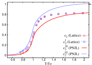
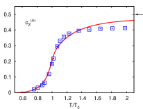
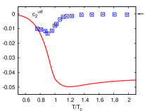
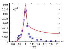
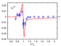
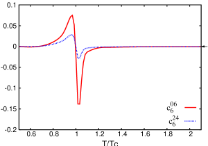
We present the QNS, INS and their higher order derivatives with respect to $\mu_{0}$ in Fig. 1. We have also plotted the LQCD data from Ref. sixx for quantitative comparison. At the second order of Taylor expansion i.e. $n=2$ we find (also observed earlier in pnjl3 ) that the QNS $c_{2}$ compares well with the LQCD data. On the other hand, the INS $c^{I}_{2}$ quickly reaches its ideal gas value above $T_{c}$ (around $2T_{c}$) in our model calculations, whereas the LQCD value are lower and matches with the value of $c_{2}$. Note that in the present form of the model the Polyakov loop itself rises a little above 1 and saturates. This leads to the INS to rise slightly above 1 at high temperatures. At the $4^{th}$ order we see that the values of $c_{4}$ (also observed in pnjl3 ) in the PNJL model matches closely with those of LQCD data for upto $T\sim 1.05T_{c}$ and deviates significantly thereafter. The coefficient $c^{I}_{4}$ is close to the LQCD data for the full range of $T$ upto $2T_{c}$.

Earlier expectation pnjl3 ; ratti3 was that, the mean field analysis may not be sufficient and hence the higher order coefficient $c_{4}$ in the PNJL model shows significant departure from lattice results. This should have also meant that the INS $c^{I}_{2}$ should be more closer to LQCD data than $c^{I}_{4}$. However, our results show that the INS $c^{I}_{2}$ is significantly different from the LQCD data above $T_{c}$, but $c^{I}_{4}$ is quite consistent. Further, we see from Fig. 1 that both the $6^{th}$ order coefficients $c_{6}$ and $c^{I}_{6}$ are quite consistent with the LQCD results. We now give a qualitative explanation for the PNJL results and try to understand the behaviour of the coefficients above $T_{c}$.

Figure 2: Left panel: $\Phi$ (solid lines) decreases and $\bar{\Phi}$ (dotted lines) increases as a function of $\mu_{0}/T$ ($\mu_{I}=0$). Right panel: $\Phi$ (solid lines) and $\bar{\Phi}$ (dotted lines) are equal and almost constant as a function of $\mu_{I}/T$ ($\mu_{0}=0$).

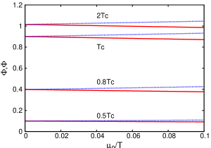
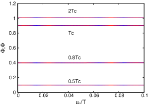
We pointed out in Section II.1 that in the thermodynamic potential Eqn. (1), the Polyakov loop couples to $\mu_{0}$ and its conjugate couples to $-\mu_{0}$ due to CP symmetry. As observed in $SU(N)$ matrix model matrix1 and also in the PNJL model pnjl2 ; pnjl3 , this difference in coupling leads to splitting of the Polyakov loop and its conjugate for any nonzero $\mu_{0}$. Thus even at high temperatures when the Polyakov loop is close to $1$, it decreases with increasing $\mu_{0}$ and its conjugate increases (see left panel of Fig. 2). This means that the $\mu_{0}$ dependence of pressure is not the same as that for an ideal gas. Hence the coefficients $c_{2}$ and $c_{4}$ are both quite off from their respective ideal gas values. Also note that though $c_{6}$ is close enough, it is still distinctly different from zero. On the other hand for $\mu_{0}=0$, the Polyakov loop as well as its conjugate couples to both the $\mu_{I}$ and $-\mu_{I}$. They are, thus, equal (see right panel of Fig. 2), and also found to be almost constant for small $\mu_{I}$. So the temperature dependence of the INS and its $\mu_{I}$ derivatives should reach the ideal gas behaviour above $T_{c}$. For the coefficients which are mixed derivatives of $\mu_{0}$ and $\mu_{I}$ the behaviour should be somewhere in between. And indeed we see that $c^{I}_{2}$, $c^{I}_{4}$ and $c^{I}_{6}$ in Fig. 1 are quite close to their respective ideal gas values above $T_{c}$. Thus the LQCD results that show almost equal values of QNS and INS, indicate that the splitting between the Polyakov Loop and its conjugate in the $\mu_{I}=0$ direction for $T>1.5T_{c}$ is almost negligible (also supported by pQCD). This splitting was taken to be absolutely zero in the recent report with the PNJL model in Ref. ratti4 .

Figure 3: The flavour diagonal (upper row) and flavour off-diagonal (lower row) susceptibilities for $n=2$, $4$ and $6$ as functions of $T/T_{c}$. Symbols are LQCD data sixx . The arrows on the right indicate the respective ideal gas values.

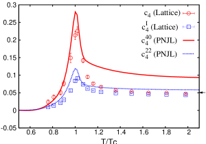
In order to investigate these discrepancies between the results form the PNJL model and the LQCD data more closely, we have also calculated the flavour diagonal ($c_{n}^{uu}$) and off-diagonal ($c_{n}^{ud}$) susceptibilities, defined in Section II.2, upto $6$-th order. These are shown in Fig. 3. Except for $c_{2}^{uu}$, all the other LQCD results for flavour diagonal susceptibilities are close to their respective ideal gas values from around $1.2T_{c}$ onwards. The PNJL model values for the diagonal coefficient $c^{uu}_{2}$ seem to be more or less consistent with the LQCD data. The most striking discrepancy with the LQCD data shows up in the $2$-nd order flavour off-diagonal susceptibility $c^{ud}_{2}$. As discussed earlier, $c_{2}^{ud}$ signifies the mixing of $u$ and $d$ quarks through the contribution of the two disconnected $u$ and $d$ quark loops. While the LQCD data shows that this kind of correlation between the $u$-$d$ flavours are almost zero just away form $T_{c}$, the PNJL model results remains significant even upto $2T_{c}$. The negativity of $c_{2}^{ud}$ (see Fig. 3) indicates that the dominant correlation is between $u$ quarks and $d$ anti-quarks and vice-verse, i.e., pion-like. Hence putting in the dynamical pion condensate may throw some light on this issue. Also addition of any new couplings (e.g. as shown for the isoscalar-vector and isovector-vector couplings for NJL model in Ref. redlich1 ) may have important consequences for these suscpetibilities.

Figure 4: $c^{04}_{4}$ and $c^{06}_{6}$ and $c^{24}_{6}$ as functions of $T/T_{c}$. Arrows on the right indicate the respective ideal gas values.

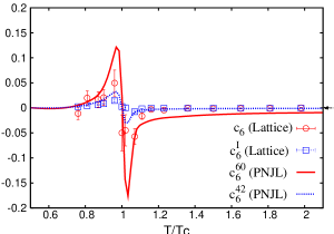
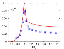
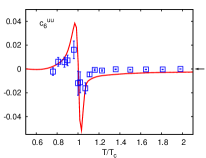
Again from Fig. 3, the $4$-th order diagonal ($c^{uu}_{4}$) as well as the off-diagonal ($c^{ud}_{4}$) coefficients show a behaviour similar to $c^{40}_{4}$. Whereas the LQCD data reaches the ideal gas value above $T_{c}$, the PNJL values are quite distinctly separated. Finally, at the $6^{th}$ order the behaviour for both diagonal and off-diagonal coefficients in the PNJL model and LQCD are quite consistent.

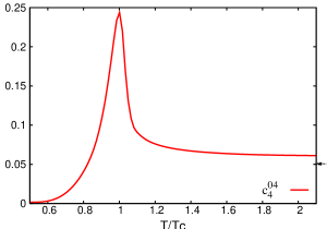
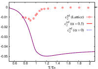
We now present the temperature dependence of the remaining nonzero coefficients (Fig. 4). $c^{04}_{4}$ is the $4$-th order diagonal coefficient in the isospin direction. In contrast to $c^{40}_{4}$ we see that $c^{04}_{4}$ approaches the ideal gas value quite fast above $T_{c}$. The behaviour of $c^{06}_{6}$ is quite similar to its counterpart $c^{60}$. This is in accordance to the expectation, as discussed earlier. Same is true for the coefficient $c^{24}_{6}$.

III.1.2 $G_{1}\neq G_{2}$

Figure 5: Left panel: $c^{ud}_{2}$ is independent of $\alpha$. Middle and Right panel: Dependence of some off-diagonal coefficients on the flavour mixing parameter $\alpha$. Symbols are Lattice data sixx . Arrows on the right indicate the corresponding ideal gas values.

Since the PNJL model has problem in reproducing the LQCD data for $c_{2}^{ud}$ which is a measure of the flavour-flavour correlation, it is interesting to have a closer look at the effect of flavour-mixing on different susceptibilities. As discussed earlier, the parameterization $G_{1}=(1-\alpha)G_{0}$ and $G_{2}=\alpha G_{0}$ enables one to tune the instanton induced flavour mixing by varying the value of $\alpha$ between 0 and 1. Here we discuss the two extreme cases of $\alpha=1$ (maximal mixing) and $\alpha=0$ (zero mixing). We have re-calculated all $c_{n}$ and $c_{n}^{I}$, upto $n=6$, for $\alpha=0,\ {\rm and},\ 1$. We found that all the diagonal coefficients, including $c^{I}_{2}$ and $c_{4}$ whose behaviour are the most drastically different in the PNJL model and in LQCD, are independent of the values of $\alpha$. As a consequence, the $2$-nd order flavour off-diagonal susceptibility [$c_{2}^{ud}=(c_{2}^{I}-c_{2})/4$] is also unaffected by the instanton induced flavour-mixing effects.

The above fact can be understood from the following reasoning. We mentioned in section II.1 that the quark condensates $\sigma_{u}$ and $\sigma_{d}$ are equal to each other for either of the cases $\mu_{0}=0$ and $\mu_{I}=0$. This is clear from Eqn. 31. Now $G_{1}$ and $G_{2}$ couple only to the $\sigma_{u}$ and $\sigma_{d}$. So for $\sigma_{u}=\sigma_{d}$, we only get the combination $G_{1}+G_{2}=G_{0}$, which is a constant. Thus none of the physics in the $\mu_{0}=0$ and $\mu_{I}=0$ directions depend on the value of $\alpha$, implying that the diagonal derivatives in these two directions will also be independent of $\alpha$.

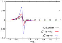
However, the mixed derivatives can have dependence on $\alpha$. This is because the values of $\sigma_{u}$ and $\sigma_{d}$ can be different when both $\mu_{0}$ and $\mu_{I}$ are together nonzero. This was seen in Ref. buballa for the normal NJL model. But those authors also found that there is a critical value of $\alpha_{c}\approx 0.11$ above which the condensates $\sigma_{u}$ and $\sigma_{d}$ become equal even for both $\mu_{0}$ and $\mu_{I}$ being nonzero. Here, for the PNJL model we have found that all the mixed derivatives upto $6^{th}$ order are exactly equal for the two cases $\alpha=0.5$ (standard mixing used in NJL and PNJL models) and $\alpha=1$ (maximal mixing) which is in accordance to the results of the above reference. We hope to obtain the value for $\alpha_{c}$ for the PNJL model in future. For $\alpha=0$ all the off-diagonal coefficients were found to differ from those at $\alpha=0.5$.

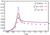
The left-most panel in Fig. 5 shows the independence of $c^{ud}_{2}$ on $\alpha$. The rest figures show one representative coefficient each for $n=4,\,{\rm and}\ 6$. As can be seen, the instanton effects quite significantly suppress the temperature variation of these coefficients near $T_{c}$. Also it can be observed from Fig. 5, that the LQCD data favours larger amount of instanton induced flavour-mixing.

III.2 Dependence of $C_{V}$ and $v_{s}^{2}$ on $\mu_{0}$ and $\mu_{I}$

Figure 6: $C_{V}$ as a function of $T/T_{c}$. Left panel shows the variation with $\mu_{0}$; Right panel shows the variation with $\mu_{I}$. Arrows on the right indicate the ideal gas value for $\mu_{0}=\mu_{I}=0$.

Figure 7: $v^{2}_{s}$ as a function of $T/T_{c}$. Left panel shows the variation with $\mu_{0}$; Right panel shows the variation with $\mu_{I}$. Arrows on the right indicate the ideal gas value for $\mu_{0}=\mu_{I}=0$.

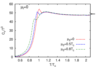
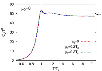
Here we present the chemical potential dependence of specific heat $C_{V}$ and the speed of sound $v_{s}$. The range of the three representative values of $\mu_{0}$ and $\mu_{I}$ are such that neither the diquark physics nor the pion condensation becomes important. In the ideal gas limit the expression for $C_{V}$ is as a function of temperature $T$ and either of the chemical potentials $\mu_{0}$ or $\mu_{I}$ is given by, $C_{V}/T^{3}=(74\pi^{2}/15)+6(\mu^{2}_{0,I}/T^{2})$. Thus, for large temperatures and not so large chemical potentials, it can be expected that the $C_{V}$ is more or less independent of $\mu_{0,I}$’s. This is borne out in the PNJL model as seen in Fig. 6. At low temperatures however, there can be non-trivial contribution from chemical potential. As illustrated in Fig. 6, the low temperature behaviour is away from ideal gas, but there is significant difference in the values of $C_{V}$ as a function of $\mu_{0}$. In the range of $\mu_{I}$ considered, even for $T<T_{c}$ there seems to no significant isospin effects. Another interesting feature is that as a function of $\mu_{0}$, the peak of $C_{V}$ which appears at $T_{c}$ shifts towards lower temperatures. This signifies that the transition temperature may decrease and also the nature of transition may change as the chemical potentials increase. A decrease of $T_{c}$ with increasing $\mu_{0}$ and $\mu_{I}$ is consistent with what have been found on the Lattice allton ; kogut1 . We hope to address this issue through the analysis of chiral susceptibility in a future publication.

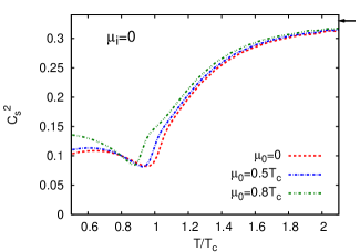
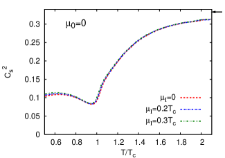
The speed of sound in the ideal gas limit is the same $\sqrt{3}$ for any given temperature and chemical potential. As shown in Fig. 7 the $v^{2}_{s}$ for different $\mu_{0}$ and $\mu_{I}$ merges towards the ideal gas value at large temperatures. However, even above $T_{c}$, there is significant increase in $v^{2}_{s}$ for increase in $\mu_{0}$. So for nonzero quark matter density the speed of sound is higher near $T_{c}$ and this may have important contribution to thermalization of the matter created in relativistic heavy-ion collision experiments. Again there seems to be negligible isospin dependence of $c^{2}_{s}$ in the range of temperatures studied. From Fig. 7 we note that in the PNJL model even with $\mu_{0}$ as large as $0.8T_{c}$, the $v^{2}_{s}$ never reaches a value as large as $0.2$ near or below $T=T_{c}$ which was used in beda to describe the rapidity spectra.

IV Discussions and Summary

We have extended the PNJL model of Ref.  pnjl2 by the introduction of isospin chemical potential. Using this we have studied the behaviour of strongly interacting matter with two degenerate quark flavours in the phase space of $T$, $\mu_{0}$ and $\mu_{I}$, for small values of the chemical potentials. We have extracted $10$ coefficients of Taylor expansion of pressure in the two chemical potentials upto $6$-th order. Some of these coefficients were compared with available LQCD data. The quark number susceptibility and isospin susceptibility show order parameter-like behaviour. A quantitative comparison shows that the quark number susceptibility reaches about $85\%$ of its ideal gas value upto temperature of about $2T_{c}$, consistent with LQCD results. However, the isospin susceptibility reaches its ideal gas value by this temperature. This is in contrast to LQCD results where both the susceptibilities are almost equal from around $1.2T_{c}$ onward. Similarly, the higher order derivatives for $\mu_{I}$ approach the the ideal gas behaviour much faster compared to those for $\mu_{0}$. In contrast, though both the QNS and INS in LQCD deviate from their ideal gas values, the higher order derivatives reach their ideal gas limit quickly. The values of the mixed derivatives in the PNJL model shows a behaviour somewhat in between. On the Lattice however, the mixed derivatives are almost zero (i.e., the ideal gas value) above $T_{c}$.

Thus some of the coefficients in the PNJL model differ from the LQCD data and one could hold the mean field analysis responsible for this departure. But if this argument were true then the higher order derivatives obtained in the PNJL model should depart from the LQCD data more than the lower order coefficients, which is not the case. As against this expectation, we have found a very nice pattern in the PNJL results which can be understood in terms of the behaviour of the Polyakov loop. The dependence of the Polyakov loop and its conjugate on temperature and the chemical potentials is extremely important. For $\mu_{I}=0$ they have different values when $\mu_{0}$ is varied. This makes all the coefficients which are derivatives of pressure with respect to $\mu_{0}$ alone, to deviate from the ideal gas behaviour. For $\mu_{0}=0$ however the Polyakov loop and its conjugate are equal and hence both reach the ideal gas value above $T_{c}$. Thus the coefficients which are derivatives of pressure with respect to $\mu_{I}$ alone, all reach their respective ideal gas values above $T_{c}$. The mixed derivatives are found to be somewhere in between. Nonetheless, we hope to look into the effects of fluctuations in future.

In order to have a closer look at the discrepancy between the PNJL results and LQCD data, we have also calculated the flavour diagonal and flavour off-diagonal susceptibilities upto $6$-th order. We have found that the $2$-nd order flavour off-diagonal susceptibility, which indicates the correlation among “up” and “down” quarks, is significantly away from zero even upto $T=2T_{c}$. On the other hand, LQCD results swagato show that correlation among the flavours in the $2$-nd order off-diagonal susceptibility is largely governed by the interaction of the quarks with the gauge fields and is almost independent of the presence of the quarks loops. This motivated us to study the instanton induced flavour-mixing effects within the framework of the PNJL model. Unfortunately, we found no effect of flavour-mixing on any diagonal QNS and INS, and hence on the $2$-nd order flavour off-diagonal susceptibility. We speculate one possibility to reconcile PNJL and LQCD data, that is to keep the pion condensate as a dynamical variable and perform the calculations. In fact there are indications kli3 that at zero temperature and in the chiral limit, pion condensation can be catalysed by an external chromomagnetic field. We hope to present these results in future.

On the other hand, flavour-mixing effects on the mixed susceptibilities of quark and isospin chemical potentials indicate that large flavour-mixing is favoured by the LQCD data. This may have important consequences buballa on the phase diagram of the NJL model at low temperature and large baryon chemical potential.

Apart from the possible improvements for the Polyakov loop potential, inclusion of pionic and diquark fluctuations, etc. we also intend to include terms in the NJL part with six point couplings to take proper account of the quark number fluctuations in the low temperature phase.

We have also investigated chemical potential dependence of specific heat and speed of sound. The specific heat sort of becomes independent of chemical potential just above $T_{c}$. Below $T_{c}$ there is some significant effect from both the chemical potentials $\mu_{0}$ and $\mu_{I}$. Consistent with LQCD findings allton ; kogut1 , the peak in specific heat towards lower temperatures with increasing chemical potentials indicating a decrease in the transition temperature. We plan to make a more detailed investigation of the location of the phase boundary. The speed of sound, on the other hand, increases with the increase of either of the chemical potentials in almost the whole range of temperatures. But this dependence become milder as one goes to higher temperatures. Thus with a proper implementation of the PNJL equation of state into the hydrodynamic studies of elliptic flow, one may able to make some estimates of both the temperature and densities reached in the heavy-ion collision experiments.

Appendix A

Here we present the complete details of the PNJL model used in our work. First we discuss the NJL model in the complete space of temperature $T$ and the “up” and “down” flavour chemical potentials $\mu_{u}$ and $\mu_{d}$ (or equivalently the quark chemical potential $\mu_{0}$ and isospin chemical potential $\mu_{I}$) asakawa1 ; buballa . Then we extend it to couple with the Polyakov Loop.

A.1 The NJL model

The NJL model Lagrangian for two flavours can be written as asakawa1 ; buballa :

$${\mathcal{L}} = {\mathcal{L}}_{0}+{\mathcal{L}}_{1}+{\mathcal{L}}_{2}~{}~{}~{},$$ (14a)

$${\mathcal{L}}_{0} = \bar{\psi}(i\partial\!\!\!/-m)\psi~{}~{}~{},$$ (14b)

$${\mathcal{L}}_{1} = G_{1}\left[\left(\bar{\psi}\psi\right)^{2}+\left(\bar{\psi}\vec{\tau}\psi\right)^{2}+\left(\bar{\psi}i\gamma_{5}\psi\right)^{2}+\left(\bar{\psi}i\gamma_{5}\vec{\tau}\psi\right)^{2}\right]~{}~{}~{},$$ (14c)

$${\mathcal{L}}_{2} = G_{2}\left[\left(\bar{\psi}\psi\right)^{2}-\left(\bar{\psi}\vec{\tau}\psi\right)^{2}-\left(\bar{\psi}i\gamma_{5}\psi\right)^{2}+\left(\bar{\psi}i\gamma_{5}\vec{\tau}\psi\right)^{2}\right]~{}~{}~{},$$ (14d)

where,

$$\psi=(u,d)^{T},\qquad\qquad[G_{1}]=[G_{2}]=[{\rm energy}]^{-2},\qquad\qquad m=diag(m_{u},m_{d}).$$ (15)

We shall assume flavour degeneracy $m_{u}=m_{d}=m_{0}$. For $m_{0}=0$ the symmetries of the different parts of the Lagrangian 14 are:

$${\mathcal{L}}_{0} : SU_{V}(2)\times SU_{A}(2)\times U_{V}(1)\times U_{A}(1)$$ (16a)

$${\mathcal{L}}_{1} : SU_{V}(2)\times SU_{A}(2)\times U_{V}(1)\times U_{A}(1)$$ (16b)

$${\mathcal{L}}_{2} : SU_{V}(2)\times SU_{A}(2)\times U_{V}(1)$$ (16c)

${\mathcal{L}}_{2}$ has the structure of a ’t-Hooft determinant, ${\rm det}\left[{\bar{q}}(1+\gamma_{5})q\right]+{\rm det}\left[{\bar{q}}(1-\gamma_{5})q\right]$ njls , and breaks $U_{A}(1)$ axial symmetry. This interaction can be interpreted as induced by instantons and reflects the $U_{A}(1)$-anomaly of QCD.

We are interested in the properties of this Lagrangian at nonzero temperatures $T$ and chemical potentials $\mu_{u}$ and $\mu_{d}$. Equivalently, one can also use the quark number chemical potential $\mu_{0}=(\mu_{u}+\mu_{d})/2$ and the isospin chemical potential $\mu_{I}=(\mu_{u}-\mu_{d})/2$. In the mean field approximation we consider the two quark condensates $\sigma_{u}=\left\langle{\bar{u}}u\right\rangle$ and $\sigma_{d}=\left\langle{\bar{d}}d\right\rangle$. The pion condensate $\vec{\pi}$ is assumed to be zero (which is true in the NJL model for $\mu_{I}<m_{\pi}/2$). Then the thermodynamic potential is obtained as,

$$\Omega(T,\mu_{u},\mu_{d}) = \sum_{f=u,d}\Omega_{0}(T,\mu_{f};m_{f})+2G_{1}\left(\sigma_{u}^{2}+\sigma_{d}^{2}\right)+4G_{2}\sigma_{u}\sigma_{d}~{}~{}~{},$$ (17a)

$$\Omega_{0}(T,\mu_{f};m_{f}) = -2N_{c}\int\frac{d^{3}p}{\left(2\pi\right)^{3}}E_{f}\theta(\Lambda^{2}-\vec{p}~{}^{2})-2N_{c}T\int\frac{d^{3}p}{\left(2\pi\right)^{3}}\ln\left[1+e^{-(E_{f}-\mu_{f})/T}\right]$$ (17b)

$$-2N_{c}T\int\frac{d^{3}p}{\left(2\pi\right)^{3}}\ln\left[1+e^{-(E_{f}+\mu_{f})/T}\right]~{}~{}~{}.$$

where, the energy $E_{f}$ and constituent quark mass $m_{f}$ is given by,

$$E_{f} = \sqrt{m_{f}^{2}+p^{2}}~{}~{},$$ (18)

$$m_{f} = m_{0}-4G_{1}\sigma_{f}-4G_{2}\sigma_{f^{\prime}},\qquad\qquad f\neq f^{\prime}\in\{u,d\}~{}~{}.$$ (19)

Finding the stationary points of the thermodynamic potential with respect to $\sigma_{u}$ and $\sigma_{d}$, i.e., solving the coupled equations $\partial\Omega/\partial\sigma_{u}=0$ and $\partial\Omega/\partial\sigma_{d}=0$, one gets the gap equations,

$$\sigma_{f}=-2N_{c}\int\frac{d^{3}p}{\left(2\pi\right)^{3}}\frac{m_{f}}{E_{f}}\left[\theta(\Lambda^{2}-p^{2})-n(E_{f})-{\bar{n}}(E_{f})\right],\qquad f={u,d}$$ (20a)

$$n(E_{f})=\frac{1}{1+\exp(E_{f}-\mu_{f})},\qquad{\rm and}\qquad{\bar{n}}(E_{f})=\frac{1}{1+\exp(E_{f}+\mu_{f})}.$$ (20b)

The constituent mass $m_{f}$ for one flavour depends in general on both the condensates [see Eqn. (19)] and therefore the two flavours are coupled. Chiral symmetry ($SU_{A}(2)$) is broken spontaneously for $\sigma_{f}\neq 0$.
Let us now make the parameterization

$$G_{1}=(1-\alpha)G_{0},\qquad{\rm and}\qquad G_{2}=\alpha G_{0}$$ (21)

with a fixed value of $G_{0}$. Tuning the value of $\alpha$ one can control the flavour mixing in the Lagrangian. We consider some of the cases below.

1. $\alpha=0$ : This implies $G_{2}=0$ i.e.the $U_{A}(1)$ symmetry breaking term ${\mathcal{L}}_{2}$ drops out and hence ${\mathcal{L}}$ has no flavour mixing.

2. $\alpha=1$ : Here $G_{1}=0$, and thus ${\mathcal{L}}_{2}$ completely dominates the coupling. The flavour mixing in ${\mathcal{L}}$ is thus “maximal”.

3. $\alpha=1/2$ : In this case we have $G_{1}=G_{2}=G_{0}/2$. So the Lagrangian ${\mathcal{L}}={\mathcal{L}}_{0}+G_{0}\left[\left(\bar{\psi}\psi\right)^{2}+\left(\bar{\psi}i\gamma_{5}\vec{\tau}\psi\right)^{2}\right]$, is the standard NJL model njl1 . Here also the $U_{A}(1)$ symmetry is broken which is commensurate with the fact that in nature the $\eta$ particle is much heavier than the $\pi$’s

A.2 Extension to PNJL

Our aim is to extend the PNJL model introduced in Ref. .pnjl1 ; pnjl2 to include isospin chemical potential. To achieve this we now include the Polyakov loop and its effective potential to the NJL model described above. The Lagrangian becomes,

$${\mathcal{L}}_{PNJL} = {\mathcal{L}}_{0}+{\mathcal{L}}_{1}+{\mathcal{L}}_{2}-{\mathcal{U}}\left(\Phi[A],\bar{\Phi}[A],T\right)$$ (22)

The only part of the NJL sector that is modified is ${\mathcal{L}}_{0}$ which now becomes,

$${\mathcal{L}}_{0}=\bar{\psi}\left(iD\!\!\!\!/-m\right)\psi~{}~{}~{},$$ (23)

where

$$D^{\mu}=\partial^{\mu}-iA^{\mu},\qquad A^{\mu}=\delta_{\mu 0}A^{0},\qquad A^{\mu}(x)=g{\mathcal{A}}^{\mu}_{a}(x)\lambda_{a}/2.$$ (24)

${\mathcal{A}}^{\mu}_{a}(x)$ are $SU(3)$ gauge fields and $\lambda_{a}$ are Gell-Mann matrices.

${\mathcal{U}}\left(\Phi[A],\bar{\Phi}[A],T\right)$ is the effective potential expressed in terms of the traced (over color) Polyakov loop (with periodic boundary conditions) and its charge conjugate—

$$\Phi=\frac{{\rm Tr}_{c}L}{N_{c}},\qquad\bar{\Phi}=\frac{{\rm Tr}_{c}L^{\dagger}}{N_{c}},\qquad L(\vec{x})={\mathcal{P}}\exp\left[i\int_{0}^{\beta}d\tau\ A_{4}(\vec{x},\tau)\right],\qquad\beta=\frac{1}{T},\qquad A_{4}=iA_{0}.$$ (25)

We shall be working in the mean field limit. For simplicity of notation we shall use $\Phi$ and $\bar{\Phi}$ as their respective mean fields. $\Phi$ is the order parameter for deconfinement transition. In the absence of quarks $\Phi=\bar{\Phi}$ and deconfinement is associated with the spontaneous breaking of the $Z(3)$ symmetry. Conforming to this symmetry and parameterizing the LQCD Monte Carlo data one can write down an effective potential for $\Phi$ and $\bar{\Phi}$. Following Ref. pnjl2 , we write

$$\frac{{\mathcal{U}}(\Phi,\bar{\Phi},T)}{T^{4}} = -\frac{b_{2}(T)}{2}\Phi\bar{\Phi}-\frac{b_{3}}{6}\left(\Phi^{3}+{\bar{\Phi}}^{3}\right)+\frac{b_{4}}{4}\left(\bar{\Phi}\Phi\right)^{2},$$ (26a)

$$b_{2}(T) = a_{0}+a_{1}\left(\frac{T_{0}}{T}\right)+a_{2}\left(\frac{T_{0}}{T}\right)^{2}+a_{3}\left(\frac{T_{0}}{T}\right)^{3}.$$ (26b)

At low temperature ${\mathcal{U}}$ has a single minimum at $\Phi=0$, while at high temperatures it develops a second one which turns into the absolute minimum above a critical temperature $T_{0}$. $\Phi$ and $\bar{\Phi}$ will be treated as independent classical fields. The mean field analysis of the NJL part of the model proceeds in exactly the same way as in the previous case. Using $\sigma_{u}$ and $\sigma_{d}$ as the independent quark condensates (and neglecting $\vec{\pi}$) one gets the expression for the thermodynamic potential,

$$\Omega(T,\mu_{u},\mu_{d}) = {\mathcal{U}}\left(\Phi,\bar{\Phi},T\right)+\sum_{f=u,d}\Omega_{0}(T,\mu_{f};M_{f})+2G_{1}\left(\sigma_{u}^{2}+\sigma_{d}^{2}\right)+4G_{2}\sigma_{u}\sigma_{d}~{}~{}~{},$$ (27a)

$$\Omega_{0}(T,\mu_{f};M_{f}) = -2N_{c}\int\frac{d^{3}p}{\left(2\pi\right)^{3}}E_{f}\theta(\Lambda^{2}-\vec{p}~{}^{2})-2T\int\frac{d^{3}p}{\left(2\pi\right)^{3}}{\rm Tr}_{c}\ln\left[1+Le^{-(E_{f}-\mu_{f})/T}\right]$$ (27b)

$$-2T\int\frac{d^{3}p}{\left(2\pi\right)^{3}}{\rm Tr}_{c}\ln\left[1+L^{\dagger}e^{-(E_{f}+\mu_{f})/T}\right]~{}~{}~{}.$$

where $E_{u,d}=\sqrt{m_{u,d}^{2}+p^{2}}$ and $m_{u,d}=m_{0}-4G_{1}\sigma_{u,d}-4G_{2}\sigma_{d,u}$.

Note that with $\alpha=0.5$ and $\mu_{u}=\mu_{d}=\mu$ and if for the coupling $G$ and condensate $\sigma$ of Ref. pnjl2 one uses $G=2G_{0}$ and $\sigma=\sigma_{u}+\sigma_{d}$, then the thermodynamic potentials here and in Ref. pnjl2 are exactly equal.

Using the identity ${\rm Tr}\ln X=\ln{\rm det}X$ one can write for a given flavour $f$,

$$\ln{\rm det}\left[1+Le^{-(E_{f}-\mu_{f})/T}\right]+\ln{\rm det}\left[1+L^{\dagger}e^{-(E_{f}+\mu_{f})/T}\right]$$

$$=\ln\left[1+3\left(\Phi+\bar{\Phi}e^{-(E_{f}-\mu_{f})/T}\right)e^{-(E_{f}-\mu_{f})/T}+e^{-3(E_{f}-\mu_{f})/T}\right]$$

$$+\ln\left[1+3\left(\bar{\Phi}+\Phi e^{-(E_{f}+\mu_{f})/T}\right)e^{-(E_{f}+\mu_{f})/T}+e^{-3(E_{f}+\mu_{f})/T}\right].$$ (28)

This gives us the final form of the thermodynamic potential as,

$$\Omega(T,\mu_{u},\mu_{d}) = {\mathcal{U}}\left(\Phi,\bar{\Phi},T\right)+\sum_{f=u,d}\Omega_{0}(T,\mu_{f};M_{f})+2G_{1}\left(\sigma_{u}^{2}+\sigma_{d}^{2}\right)+4G_{2}\sigma_{u}\sigma_{d},$$ (29a)

$$\Omega_{0}(T,\mu_{f};M_{f}) = -2N_{c}\int\frac{d^{3}p}{\left(2\pi\right)^{3}}E_{f}\theta(\Lambda^{2}-\vec{p}~{}^{2})$$ (29b)

$$-2T\int\frac{d^{3}p}{\left(2\pi\right)^{3}}\ln\left[1+3\left(\Phi+\bar{\Phi}e^{-(E_{f}-\mu_{f})/T}\right)e^{-(E_{f}-\mu_{f})/T}+e^{-3(E_{f}-\mu_{f})/T}\right]$$

$$-2T\int\frac{d^{3}p}{\left(2\pi\right)^{3}}\ln\left[1+3\left(\bar{\Phi}+\Phi e^{-(E_{f}+\mu_{f})/T}\right)e^{-(E_{f}+\mu_{f})/T}+e^{-3(E_{f}+\mu_{f})/T}\right]~{}~{}~{}.$$

From this thermodynamic potential the equations of motion for the mean fields $\sigma_{u}$, $\sigma_{d}$, $\Phi$ and $\bar{\Phi}$ are derived through,

$$\frac{\partial\Omega}{\partial\sigma_{u}}=0,\qquad\frac{\partial\Omega}{\partial\sigma_{d}}=0,\qquad\frac{\partial\Omega}{\partial\Phi}=0,\qquad\frac{\partial\Omega}{\partial\bar{\Phi}}=0.$$ (30)

This coupled equations are then solved for the fields as functions of $T$, $\mu_{u}$ and $\mu_{d}$. They give,

$$\sigma_{f} = -6\int\frac{d^{3}p}{(2\pi)^{3}}\frac{m_{f}}{E_{f}}\left[\theta(\Lambda^{2}-p^{2})-{\mathcal{N}}(E_{f}){\mathcal{M}}(E_{f})-\bar{\mathcal{N}}(E_{f})\bar{\mathcal{M}}(E_{f})\right];\qquad f=u,d$$ (31a)

$$\frac{\partial{\mathcal{U}}}{\partial\Phi} = 6T\sum_{f=u,d}\int\frac{d^{3}p}{(2\pi)^{3}}\left[{\mathcal{N}}(E_{f})e^{-(E_{f}-\mu_{f})/T}+\bar{\mathcal{N}}(E_{f})e^{-2(E_{f}+\mu_{f})/T}\right],$$ (31b)

$$\frac{\partial{\mathcal{U}}}{\partial\bar{\Phi}} = 6T\sum_{f=u,d}\int\frac{d^{3}p}{(2\pi)^{3}}\left[{\mathcal{N}}(E_{f})e^{-2(E_{f}-\mu_{f})/T}+\bar{\mathcal{N}}(E_{f})e^{-(E_{f}+\mu_{f})/T}\right],$$ (31c)

$${\mathcal{N}}(E_{f}) = \left[1+3\left(\Phi+\bar{\Phi}e^{-(E_{f}-\mu_{f})/T}\right)e^{-(E_{f}-\mu_{f})/T}+e^{-3(E_{f}-\mu_{f})/T}\right]^{-1},$$ (31d)

$$\bar{\mathcal{N}}(E_{f}) = \left[1+3\left(\bar{\Phi}+\Phi e^{-(E_{f}+\mu_{f})/T}\right)e^{-(E_{f}+\mu_{f})/T}+e^{-3(E_{f}+\mu_{f})/T}\right]^{-1},$$ (31e)

$${\mathcal{M}}(E_{f}) = \left(\Phi+2\bar{\Phi}e^{-(E_{f}-\mu_{f})/T}\right)e^{-(E_{f}-\mu_{f})/T}+e^{-3(E_{f}-\mu_{f})/T},$$ (31f)

$$\bar{\mathcal{M}}(E_{f}) = \left(\bar{\Phi}+2\Phi e^{-(E_{f}+\mu_{f})/T}\right)e^{-(E_{f}+\mu_{f})/T}+e^{-3(E_{f}+\mu_{f})/T}.$$ (31g)

Finally we note that the values of the parameters used are exactly the same as used in Ref. pnjl3 .