Folded Supersymmetry and the LEP Paradox

Abstract

We present a new class of models that stabilize the weak scale against radiative corrections up to scales of order 5 TeV without large corrections to precision electroweak observables. In these ‘folded supersymmetric’ theories the one loop quadratic divergences of the Standard Model Higgs field are cancelled by opposite spin partners, but the gauge quantum numbers of these new particles are in general different from those of the conventional superpartners. This class of models is built around the correspondence that exists in the large $N$ limit between the correlation functions of supersymmetric theories and those of their non-supersymmetric orbifold daughters. By identifying the mechanism which underlies the cancellation of one loop quadratic divergences in these theories, we are able to construct simple extensions of the Standard Model which are radiatively stable at one loop. Ultraviolet completions of these theories can be obtained by imposing suitable boundary conditions on an appropriate supersymmetric higher dimensional theory compactified down to four dimensions. We construct a specific model based on these ideas which stabilizes the weak scale up to about 20 TeV and where the states which cancel the top loop are scalars not charged under Standard Model color. Its collider signatures are distinct from conventional supersymmetric theories and include characteristic events with hard leptons and missing energy.

I Introduction

Precision electroweak measurements performed at LEP over the past decade, while lending strong support to the Standard Model (SM), have lead to an apparent paradox LEPparadox . These experiments are completely consistent with

• the existence of a light SM Higgs with mass less than about 200 GeV, and also

• a cutoff $\Lambda$ for non-renormalizable operators that contribute to the precision electroweak observables greater than or of order 5 TeV.

The problem arises because quadratically divergent loop corrections from scales of order 5 TeV, particularly from diagrams involving the top quark, naturally generate a Higgs mass much larger than 200 GeV in the SM. This is called the ‘LEP paradox’.

The LEP paradox seems to suggest the existence of new physics at or below a TeV that cancels quadratically divergent contributions to the Higgs mass, but does not contribute significantly to precision electroweak observables. One interesting possibility is weak scale supersymmetry, where R-parity ensures that contributions to precision electroweak observables are small. Here the quadratically divergent contributions to the Higgs mass from the top quark are cancelled by new diagrams involving the scalar stops, shown in Figure (1).

Little Higgs theories Little1 ; Little2 constitute another approach to the LEP paradox. Models of this type with a custodial SU(2) custodial and T-parity Tparity do not give large corrections to precision electroweak observables. Warped extra-dimensional realizations of the Higgs as a pseudo-Goldstone boson CNP are closely related to little Higgs theories. Reviews of this class of models and more references may be found in Reviews . In little Higgs theories the top loop is cancelled by diagrams involving new fermions, the ‘top-partners’, which are charged under color and whose couplings to the Higgs are related by symmetry to the top Yukawa coupling. These diagrams are also shown in Figure (1).

Recently twin Higgs theories twin twinLR , (see also CHWtwin ,FPStwin ), a new class of solutions to the LEP paradox, have been proposed. These models have the feature that the diagrams which cancel the top loop have exactly the same form as in little Higgs theories, but the top-partners are not necessarily charged under SM color. The reason is that in a twin Higgs theory the top-partners need be related to the SM top quarks only by a discrete symmetry and not by a global symmetry as in little Higgs theories, and so do not necessarily carry the same color charge. Clearly, what is crucial for the cancellation to go through is that the couplings of the top-partners to the Higgs be related by symmetry in a specific way to the top Yukawa coupling. In these diagrams color serves merely as a multiplicity factor, and therefore whether the top-partners are charged under SM color or not is irrelevant to the cancellation.

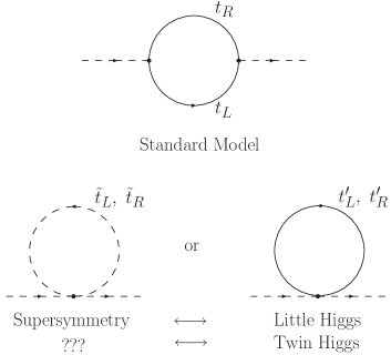
Figure 1: The diagram on top shows the contribution to the Higgs mass squared parameter in the SM from the top loop, while the lower two diagrams show how this contribution is cancelled in supersymmetric theories and in little Higgs theories. In twin Higgs models the cancellation takes place through a diagram of the same form as in the little Higgs case but the particles running in the loop need not be charged under color. In analogy with this, we seek a theory where the cancellation takes the same form as in the supersymmetric diagram but the states in the loop are not charged under color.

At this point we turn our attention back to the supersymmetric case, where the cancellation of the top loop is realized by the scalar stops. Note that the fact that the stops are charged under SM color does not seem crucial for this cancellation, any more than in the little Higgs case. As before, color seems to serve merely as a multiplicity factor and what is necessary for the cancellation to go through is that the couplings of the scalars to the Higgs be related by symmetry in a specific way to the top Yukawa coupling. This observation begs the following question. Do there exist realistic theories where the quadratic divergence from the top loop is cancelled by a diagram of the same form as in the supersymmetric case, but where the scalars running in the loop are not charged under SM color?

The purpose of this paper is to answer this question firmly in the affirmative. We will construct a realistic model where the top loop is cancelled by scalars not charged under color. Moreover, in doing so we will go much further and outline the general construction of simple extensions of the SM where one loop quadratically divergent contributions to the Higgs mass from gauge and Yukawa interactions are cancelled by opposite spin partners whose gauge quantum numbers can in principle be very different from those of the conventional superpartners. We expect these results to enable the construction of entirely new classes of models that address the LEP paradox.

Our starting point is the observation that in the large $N$ limit a relation exists between the correlation functions of a class of supersymmetric theories and those of their non-supersymmetric orbifold daughters that holds to all orders in perturbation theory fold1 ; fold2 ; fold3 ; fold4 . The masses of scalars in the daughter theory are protected against quadratic divergences by the supersymmetry of the mother theory. In many cases the correspondence between the mother and daughter theories continues to hold to a good approximation even away from the large $N$ limit. By understanding the dynamics which underlies this cancellation, we can construct simple non-supersymmetric extensions of the SM where the Higgs mass is protected from large radiative corrections at one loop. These theories stabilize the weak scale against radiative corrections up to about 5 TeV, thereby addressing the LEP paradox.

In general, the low energy spectrum of such a ‘folded supersymmetric’ theory is radically different from that of a conventional supersymmetric theory, and the familiar squarks and gauginos need not be present. While the diagrams that cancel the one loop quadratically divergent contributions to the Higgs mass have exactly the same form as in the corresponding supersymmetric theory, the gauge quantum numbers of the particles running in the loops, the ‘folded superpartners’ (or ‘F-spartners’ for short), need not be the same. This means that the characteristic collider signatures of folded supersymmetric theories tend to be distinct from those of more conventional supersymmetric models.

A folded supersymmetric theory does not in general possess any exact or approximate symmetry that guarantees that the form of the Lagrangian is radiatively stable. It is therefore particularly important to understand if ultraviolet completions of these theories exist. We show that supersymmetric ultraviolet completions where corrections to the Higgs mass from states at the cutoff are naturally small can be obtained by imposing suitable boundary conditions on an appropriate supersymmetric higher dimensional theory compactified down to four dimensions. We investigate in detail one specific model constructed along these lines. While in this theory the one loop radiative corrections to the Higgs mass from gauge loops are cancelled by gauginos, the corresponding radiative corrections from top loops are cancelled by particles not charged under SM color. In such a scenario the familiar supersymmetric collider signatures associated with the decays of squarks and gluinos that have been pair produced are absent. Instead, the signatures include events with hard leptons and missing energy that can potentially be identified at the LHC.

This paper is organized as follows. In the next section we explain the basics of orbifolding supersymmetric large $N$ theories to non-supersymmetric ones and give some simple examples establishing the absence of one loop quadratically divergent radiative corrections to scalar masses in the daughter theories. Based on these examples we then identify the underlying dynamics behind these cancellations, and explain how to extend these results to construct larger classes of theories where one loop quadratic divergences are also absent. In section III we apply these methods to show how the quadratic divergences of the Higgs in the SM can be cancelled, and outline ultraviolet completions of these theories based on Scherk-Schwarz supersymmetry breaking on higher dimensional orbifolds. In section IV we present a realistic ultraviolet complete model based on these ideas and briefly discuss its phenomenology.

II Cancellation of Divergences in Orbifolded Theories

What is the procedure to orbifold a parent supersymmetric field theory? First, identify a discrete symmetry of the parent theory. In order to obtain a non-supersymmetric daughter theory this discrete symmetry should be an R symmetry. Now ‘orbifolding’ simply consists of eliminating all fields of the parent theory that are not invariant under the discrete symmetry. The interactions of the daughter theory are inherited from the Lagrangian of the parent theory by keeping all terms which involve only the daughter fields. We will begin by demonstrating this procedure in two examples, one with gauge interactions and one with Yukawa interactions. Then, in subsection II.2 we will identify the mechanism that guarantees the cancellation of divergences at one loop and list the ‘rules’ for building models where such a cancellation is realized.

II.1 Examples of Orbifold Theories

To clarify this procedure we apply it to orbifold a supersymmetric U(2$N$) gauge theory with 2$N$ flavors down to a non-supersymmetric daughter theory with a U($N$) $\times$ U($N$) gauge symmetry. The SU(2$N$) and U(1) component gauge fields of U(2$N$) are assumed to have the same strength when their generators are normalized appropriately. The U(2$N$) theory is invariant under a discrete $Z_{2}$ symmetry which is an element of the gauge group and is generated by a matrix $\Gamma$ that has the form

$$\pmatrix{+1&&&&&\cr&\ddots&&&&\cr&&+1&&&\cr&&&-1&&\cr&&&&\ddots&\cr&&&&&-1}$$ (1)

Under this symmetry the superfields transform as $Q\rightarrow\Gamma Q$, $\bar{Q}\rightarrow\Gamma^{*}\bar{Q}$, and $V\rightarrow\Gamma V\Gamma^{\dagger}$. Here $V$ is the vector superfield while $Q$ and $\bar{Q}$ are chiral superfields which transform as the fundamental and anti-fundamental representations of U(2$N$), and the matrix $\Gamma$ is acting on the gauge indices of $Q$ and $\bar{Q}$. We label this symmetry by $Z_{2\Gamma}$. The theory is further invariant under a different discrete $Z_{2}$ symmetry which is an element of the U($2N$) $\times$ U($2N$) flavor symmetry and which is generated by a matrix F of the form

$$\pmatrix{+1&&&&&\cr&\ddots&&&&\cr&&+1&&&\cr&&&-1&&\cr&&&&\ddots&\cr&&&&&-1}$$ (2)

Under this symmetry, which we denote by $Z_{2{\rm{\bf F}}}$, the superfields $Q$ and $\bar{Q}$ transform as $Q\rightarrow Q{\rm{\bf F}}^{\dagger}$, $\bar{Q}\rightarrow\bar{Q}{\rm{\bf F}}^{T}$. Here the matrix F acts on the flavor indices of $Q$ and $\bar{Q}$, and not the color indices. Finally, the theory is invariant under a $Z_{2R}$ discrete symmetry under which all bosonic components of the superfields are even while all fermionic components are odd. Under the combined $Z_{2\Gamma}\times Z_{2{\rm{\bf F}}}\times Z_{2R}$ symmetry each field in any given supermultiplet is either even or odd. Specifically, for the components of the vector superfield $V$ of U(2$N$)

$$A_{\mu} = \pmatrix{A_{\mu,AA}(+)&A_{\mu,AB}(-)\cr A_{\mu,BA}(-)&A_{\mu,BB}(+)}$$

$$\lambda = \pmatrix{\lambda_{AA}(-)&\lambda_{AB}(+)\cr\lambda_{BA}(+)&\lambda_{BB}(-)}$$ (3)

Here $A$ and $B$ distinguish between the two U($N$) gauge groups that are contained in the original U(2$N$) gauge group. The plus and minus signs in brackets indicate whether the corresponding field is even or odd under the discrete symmetry. For the components of the chiral superfield $Q$

$$\tilde{q} = \pmatrix{\tilde{q}_{Aa}(+)&\tilde{q}_{Ab}(-)\cr\tilde{q}_{Ba}(-)&\tilde{q}_{Bb}(+)}$$

$$q = \pmatrix{q_{Aa}(-)&q_{Ab}(+)\cr q_{Ba}(+)&q_{Bb}(-)}$$ (4)

Here $a$ and $b$ distinguish between the two U($N$) flavor groups that are contained in the original U(2$N$) flavor group. The components of $\overline{Q}$ have exactly the same transformation properties as the corresponding components in $Q$.

We orbifold the supersymmetric U(2$N$) gauge theory down to a non-supersymmetric U($N$) $\times$ U($N$) daughter gauge theory by keeping in the Lagrangian only those fields invariant under the combined $Z_{2\Gamma}\times Z_{2{\rm{\bf F}}}\times Z_{2R}$ symmetry. At the same time the gauge coupling constant of the daughter theory is rescaled to be a factor of $\sqrt{2}$ larger than the corresponding coupling constant in the mother theory. It has been shown in fold4 that in the large N limit the correlation functions of this daughter theory are equal (up to rescalings) to the corresponding correlation functions of the supersymmetric parent theory. This result holds to all orders in perturbation theory.

This implies that in the large $N$ limit, quadratically divergent contributions to the mass squared of the scalar $\tilde{q}_{Aa}$ are absent in the daughter theory. It is straightforward to verify this at one loop. From the couplings to the gauge bosons $A_{\mu,AA}$ of SU($N$) and U(1) we obtain quadratically divergent contributions $(3/32\pi^{2})g^{2}\Lambda^{2}(N-1/N)$ and $(3/32\pi^{2})g^{2}\Lambda^{2}(1/N)$ respectively. Here $g$ is the gauge coupling constant in the daughter theory and $\Lambda$ is a hard cutoff scale. From the scalar self-interactions that survive from the D-term of U(2$N$) we obtain $1/32\pi^{2}g^{2}\Lambda^{2}N$. Only $\lambda_{AB}$ and $\lambda_{BA}$, the off-diagonal components of the gauginos $\lambda$, survive after orbifolding. These contribute $-(1/8\pi^{2})g^{2}\Lambda^{2}N$ to the mass of $\tilde{q}_{Aa}$. The sum total is exactly zero, as expected from the non-renormalization theorem. What if we had started with SU(2$N$) instead of U(2$N$)? Then the cancellation would have been only partial, and the contribution to the scalar mass would have been $-(1/16\pi^{2})g^{2}\Lambda^{2}(1/N)$, which vanishes in the large $N$ limit but not otherwise.

It is important to note that in the orbifolded theory the relation between the gauge coupling constant, the scalar-fermion-gaugino coupling and the scalar self coupling that are crucial to this cancellation do not immediately follow from any symmetry principle. Therefore it is important that an ultraviolet completion exist that guarantees the relation between these different couplings at some ultraviolet scale. We will defer the problem of finding such ultraviolet completions to the next section.

Can the correspondence be extended to theories with Yukawa couplings? For certain classes of theories where all matter is in bifundamentals, this is straightforward. Consider a supersymmetric theory with an SU(2$N)_{1}\times$ SU(2$N)_{2}\times$ SU(2$N)_{3}$ global symmetry and matter content $Q_{12}=(2N,\overline{2N},1),Q_{23}=(1,2N,\overline{2N}),Q_{31}=(\overline{2N},1,2N)$. This choice of global symmetries admits the Yukawa interaction

$$\lambda\;Q_{12}\;Q_{23}\;Q_{31}$$ (5)

in the superpotential. The Lagrangian is then invariant under a discrete $Z_{2\Gamma}$ symmetry where the superfields $Q_{12}$, $Q_{23}$ and $Q_{23}$ transform as $Q_{12}\rightarrow\Gamma Q_{12}\Gamma^{\dagger}$, $Q_{23}\rightarrow\Gamma Q_{23}\Gamma^{\dagger}$ and $Q_{31}\rightarrow\Gamma Q_{31}\Gamma^{\dagger}$, in a notation where $\Gamma$ always acts on the SU(2$N$) index and $\Gamma^{\dagger}$ on the SU$(\overline{2N})$ of the $Q$’s. The theory is also invariant under a $Z_{2R}$ discrete symmetry under which the bosonic components of each superfield are even while the fermionic components are odd. We can obtain a daughter theory with [SU($N)_{1A}\times$ SU($N)_{1B}\times$ SU($N)_{2A}\times$ SU($N)_{2B}\times$ SU($N)_{3A}\times$ SU($N)_{3B}$] global symmetry by projecting out of the theory those states that are odd under the combined $Z_{2\Gamma}\times Z_{2R}$ symmetry. Here $A$ and $B$ again distinguish between the two SU($N$) groups which emerge from each of the original SU(2$N$) groups. Under the action of the combined symmetry the components of $Q_{12}$ transform as shown below.

$$\tilde{q}_{12}=\pmatrix{\tilde{q}_{1A,2A}(+)&\tilde{q}_{1A,2B}(-)\cr\tilde{q}_{1B,2A}(-)&\tilde{q}_{1B,2B}(+)}$$

$$q_{12}=\pmatrix{q_{1A,2A}(-)&q_{1A,2B}(+)\cr q_{1B,2A}(+)&q_{1B,2B}(-)}$$ (6)

The transformation of the components of $Q_{23}$ and $Q_{31}$ under the combined symmetry is identical to that of the corresponding components of $Q_{12}$. We also rescale $\lambda\rightarrow\sqrt{2}\lambda$ in the daughter theory. Then, using the methods of fold4 it can be shown that the correlation functions of the mother and daughter theories are related to all orders in perturbation theory, in exact analogy to the gauge theory case we studied previously.

Let us again verify the cancellation of one loop quadratically divergent contributions to the mass of the scalars in the daughter theory. For simplicity, we focus on corrections to the mass of $\tilde{q}_{1A,2A}$. Schematically, the relevant couplings are

$$\left[\;\sqrt{2}\lambda\;\tilde{q}_{1A,2A}\;q_{2A,3B}\;q_{3B,1A}\;+\;{\rm h.c.}\;\right]\;\;+\;\;\;$$

$$2\;\lambda^{2}\;|\tilde{q}_{1A,2A}|^{2}\;|\tilde{q}_{3A,1A}|^{2}+2\;\lambda^{2}\;|\tilde{q}_{1A,2A}|^{2}\;|\tilde{q}_{2A,3A}|^{2}$$ (7)

It is easy to see that just as in supersymmetry, the contributions from the scalar loops cancel against the fermion loop so that the net one loop correction to the mass of $\tilde{q}_{1A,2A}$ vanishes identically, even for small $N$. Similar cancellations extend to the masses of all other scalars in the theory. The correspondence implies that this cancellation goes through to all loop orders at large $N$.

II.2 The Underlying Mechanism and Bifold Protection

In general, the class of theories to which the large $N$ orbifold correspondence applies is rather restricted, which would seem to limit its application to the problem of stabilizing the weak scale. However, in order to address the LEP paradox it is sufficient that the quadratic divergences of the SM be cancelled at one loop, and then again only for one specific field - the Higgs. If we can identify the origin of the cancellation of one loop quadratic divergences in the non-supersymmetric daughter theories above, it may be possible to apply the same underlying principles to construct much larger classes of theories which are radiatively stable at one loop.

What then underlies the cancellation of one loop quadratic divergences in the examples we have considered? The key observation is that in each case the scalar mass in the mother theory enjoys bifold protection. Consider one loop quadratically divergent corrections to the scalar mass in the mother theory. For any given graph the states running in the loop each carry two large $N$ indices. One of these indices, which we label $`i^{\prime}$, is summed over from 1 to $2N$, while the other index is unsummed. Consider the contribution arising from bosons running in the loop, with the summed index $i$ running from 1 to $N$. This can be thought of as being cancelled either by the fermion loop with $i$ again running from 1 to $N$ or by the fermion loop with $i$ instead running from $N+1$ to $2N$. The first cancellation is an immediate consequence of supersymmetry. The second follows from the combination of supersymmetry and additional global, gauge or discrete symmetries that these theories possess. Then by projecting out of the theory those bosons with index $i$ running from $N+1$ through $2N$, and also those fermions with index $i$ running from 1 through $N$, the cancellation still goes through. This explains the absence of one loop quadratic divergences to the scalar mass in the daughter theory.

Based on this observation, we are now in a position to outline a set of procedures which suitably extend the particle content and vertices of a theory so as to cancel the leading one loop quadratic divergence to the mass of a scalar arising from a specific interaction. The ‘rules’ below apply in most simple cases, including those we will be considering.

• Supersymmetrize.

• In the relevant graphs identify an index as being summed over from 1 to $N$. Then extend the particle content and gauge, global or discrete symmetries of the theory so that this index runs from 1 to 2$N$, while the vertices in each graph otherwise remain the same. For the cases of SU($N$) gauge interactions and Yukawa interactions, this can always be done in such a way that the scalar mass parameter in the resulting theory enjoys bifold protection, and is invariant under $Z_{2\Gamma}$ and $Z_{2R}$ symmetries.

• Project out states odd under the combined $Z_{2\Gamma}\times Z_{2R}$ symmetry. The resulting daughter theory is free of one loop quadratic divergences, up to potential (1/$N$) corrections.

When applied to SU(N) gauge interactions, or to Yukawa interactions, an ultraviolet completion can always be found for the daughter theory that is consistent with this cancellation. We will see how to construct such ultra-violet completions in the next section.

We now provide an example of how to apply these rules. Consider a theory consisting of a scalar singlet $S$ that has a Yukawa coupling to chiral fermions $Q_{i}$ and $\bar{Q}_{i}$ which transform as the fundamental and anti-fundamental representations of a global U($N$) symmetry. Here the index $i$ runs from 1 to $N$. The Yukawa coupling takes the form

$$\lambda\;S\;Q_{i}\;\overline{Q}_{i}$$ (8)

We wish to extend this theory so as to cancel quadratic divergences to the scalar mass from this Yukawa interaction. We first supersymmetrize so that $S$, $Q_{i}$ and $\bar{Q}_{i}$ are all promoted to chiral superfields and the Yukawa interaction above is now in the superpotential. We identify $i$ as the large $N$ index since it is summed over in the loop which contributes to the mass of $S$. We therefore promote the global U($N$) symmetry to a global U($2N$) symmetry by adding extra $Q$’s and $\bar{Q}$’s to the theory so that the index $i$ now runs from 1 to $2N$, while the Yukawa coupling above has exactly the same form as above. In the resulting theory the mass of the scalar $S$ clearly enjoys bifold protection. The theory also possesses a $Z_{2\Gamma}$ symmetry under which the singlet $S$ is invariant while $Q\rightarrow-\Gamma Q$, $\bar{Q}\rightarrow-\Gamma^{*}\bar{Q}$, and a $Z_{2R}$ symmetry under which all bosonic fields are even while all fermionic fields are odd. If we project out all fields odd under the combined $Z_{2\Gamma}\times Z_{2R}$ symmetry, it is straightforward to verify that in the daughter theory quadratically divergent contributions to the mass of $S$ vanish even though the theory is not supersymmetric. However, note that quadratically divergent contributions to the mass of the scalars in $Q$ and $\bar{Q}$ in the daughter theory, while large $N$ suppressed, do not in fact cancel at all. This will feed into the mass of $S$ at one higher loop order, and therefore the procedure we have outlined to protect the mass of the scalar $S$ does not extend beyond one loop. However, as we have explained, this is perfectly sufficient to address the LEP paradox.

III Application to the Standard Model

In this section we apply these ideas to the problem of stabilizing the weak scale. We limit ourselves to finding appropriate orbifolds and their ultraviolet completions, while postponing the discussion of completely realistic models to the next section. The Higgs mass parameter in the SM receives one loop quadratically divergent contributions from gauge, Yukawa and quartic self-interactions. Of these the contribution from the top Yukawa coupling is numerically the most significant by about an order of magnitude, and we therefore consider it first. We then go on to consider a model where the dominant part of the one loop quadratic divergence from the gauge interactions is cancelled.

III.1 The Top Yukawa Coupling

Choice of Orbifold

After supersymmetrization the top Yukawa interaction has the form

$$\lambda_{t}\left(3,2\right)_{Q_{3}}\left(1,2\right)_{H_{U}}\left(\overline{3},1\right)_{U_{3}}$$ (9)

in the superpotential. Here $Q_{3}$ represents the third generation SU(2) doublet containing the top and bottom quarks, $H_{U}$ the up-type Higgs and $U_{3}$ the SU(2) singlet (anti)top-quark. If we treat both SU(2) indices $i$ and SU(3) indices $\alpha$ as large $N$ indices, in t’Hooft double line notation the top quark contribution to the Higgs mass parameter takes the form shown in Figure (2).

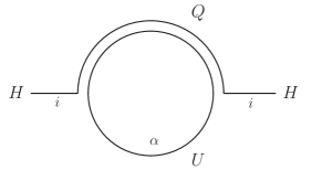
Figure 2: The top loop diagram for the Higgs mass in double line notation. In order to give the Higgs bifold protection SU(3) color, represented by the index $\alpha$, may be extended to SU(6) or to SU(3$)\times$ SU(3$)\times Z_{2}$.

From the figure, it is clear that it is the SU(3) indices $\alpha$ which are being summed over. In order to obtain a theory where the Higgs mass enjoys bifold protection we must double this sum. This can be done in either of two ways, which have somewhat different phenomenology.

• Extend the gauge symmetry from SU(3) to SU(6). This is the approach we shall follow for the rest of this section.

• Extend the gauge symmetry from SU(3) to [SU(3) $\times$ SU(3)], with a discrete symmetry interchanging the two SU(3) gauge groups. We will consider this approach in section IV.

After extending the SU(3) color gauge symmetry of the SM to an SU(6) gauge symmetry, the top Yukawa coupling has the form

$$\lambda_{t}\left(6,2\right)_{{Q}_{3T}}\left(1,2\right)_{H_{U}}\left(\overline{6},1\right)_{{U}_{3T}}$$ (10)

Here the field ${{Q}_{3T}}$ contains not only ${Q_{3}}$ of the SM but also exotic fields charged under SU(2$)_{\rm L}$ and U(1$)_{\rm Y}$ but not under SM color. Similarly ${{U}_{3T}}$ contains not only ${U_{3}}$ of the SM but also exotic fields charged under U(1$)_{\rm Y}$ but not under SM color. We refer to these new fields as the ‘folded partners’ (or ‘F-partners’ for short) of the corresponding MSSM fields. Now the theory is invariant under a $Z_{2\Gamma}$ symmetry under which ${{Q}_{3T}}\rightarrow-\Gamma{{Q}_{3T}}$, ${{U}_{3T}}\rightarrow-\Gamma^{*}{{U}_{3T}}$, $V_{6}\rightarrow\Gamma V_{6}\Gamma^{\dagger}$. Here $V_{6}$ is the vector superfield corresponding to the SU(6) gauge group. The form of the matrix $\Gamma$ is as shown in Eq. (1). We temporarily defer the question of how this symmetry is extended to the other fields in the MSSM. The theory also possesses a $Z_{2R}$ symmetry under which all fermionic fields are odd and all bosonic fields even.

Now consider the transformation properties of the various fields under the combined $Z_{2\Gamma}\times Z_{2R}$ symmetry.

$$\tilde{q}_{3T}=\pmatrix{\tilde{q}_{\alpha}(-)\cr\tilde{q}_{\beta}(+)}\;\;\;\;q_{3T}=\pmatrix{q_{\alpha}(+)\cr q_{\beta}(-)}$$ (11)

Here $\alpha$ and $\beta$ distinguish between the two SU(3) subgroups of SU(6) which are left unbroken under this operation. Similarly

$$\tilde{u}_{3T}=\pmatrix{\tilde{u}_{\alpha}(-)\cr\tilde{u}_{\beta}(+)}\;\;\;\;u_{3T}=\pmatrix{u_{\alpha}(+)\cr u_{\beta}(-)}$$ (12)

while the scalar and fermion components of $H_{U}$ are even and odd respectively.

$$H_{U}=\left(h_{u}(+),\tilde{h}_{u}(-)\right)$$ (13)

After orbifolding out the odd states, consider the quadratically divergent contributions to the mass parameter of the up-type Higgs field. The relevant interactions have the form

$$\left[\;\lambda_{t}\;h_{u}\;q_{\alpha}\;u_{\alpha}\;+\;{\rm h.c.}\;\right]\;\;+\;\;\;$$

$$\lambda_{t}^{2}\;|\tilde{q}_{\beta}h_{u}|^{2}+\lambda_{t}^{2}\;|\tilde{u}_{\beta}|^{2}\;|h_{u}|^{2}$$ (14)

Then quadratically divergent contributions from scalar loops cancel against those from fermion loops. Note, however that the scalar fields responsible for this cancellation are not charged under SM color, but under a different, hidden color group.

What about quadratically divergent contributions to the masses of the F-squarks $\tilde{q}_{\beta}$ and $\tilde{u}_{\beta}$? It is easy to see that these do not cancel, because these fields do not have any couplings to fermions in the daughter theory. This implies that there will be quadratically divergent contributions to the mass of the Higgs at two loops. This is an illustration of the fact that for general orbifolds the daughter theory does not possess any symmetry that can guarantee radiative stability of the parameters to all orders. For this reason it is important that the daughter theory possess an ultraviolet completion that can set the values of the parameters at the high scale.

An Ultraviolet Completion

We now outline an ultraviolet completion that sets the couplings of the Higgs field in the low energy effective theory to their folded-supersymmetric values. Consider a five-dimensional supersymmetric theory with an extra dimension of radius $R$ compactified on $S^{1}/Z_{2}$, with branes at the orbifold fixed points. The locations of the branes are at $y=0$ and $y=\pi R$, where $y$ denotes the coordinates of points in the fifth dimension. The gauge symmetry is SU(6$)\times$ SU(2$)\times$ U(1), and all gauge fields live in the bulk of the higher dimensional space. The SU(6) gauge symmetry is broken to SU(3$)\times$ SU(3$)\times$ U(1) by boundary conditionsstringorbifolds ; Kawamura ; Altarelli ; Hall . At the same time supersymmetry is broken by the Scherk-Schwarz mechanismS&S ; P&Q ; APQ ; BHN so that while physics on each brane respects a (different) four dimensional $\mathcal{N}=1$ supersymmetry, below the compactification scale supersymmetry is completely broken. The Higgs fields $H_{U}$ and $H_{D}$ are localized on the brane where SU(6) is preserved. However all matter fields emerge from hypermultiplets which live in the bulk of the space. To specify the boundary conditions to be satisfied by bulk fields we need to know their transformation properties under reflections about $y=0$, which we denote by $Z$. In addition, we also need to specify either their transformation properties under translations by $2\pi R$, which we denote by $T$, or their transformation properties under reflections about $\pi R$, which we denote by $Z^{\prime}$. $T$ and $Z^{\prime}$ are related by $Z^{\prime}=T\;Z$. We choose to describe the boundary conditions satisfied by the various fields in terms of $Z$ and $Z^{\prime}$.

A supersymmetric gauge multiplet $\hat{V}$ in five dimensions consists of $A_{M},\lambda,\lambda^{\prime}$ and $\sigma$. From the four dimensional viewpoint the five dimensional theory has $\mathcal{N}=2$ supersymmetry. Under the action of $Z$ this $\mathcal{N}=2$ supersymmetry is broken to $\mathcal{N}=1$ supersymmetry. The five dimensional multiplet can be broken up into four dimensional $\mathcal{N}=1$ supermultiplets as $\hat{V}=\left(V,\Sigma\right)$ where $V$ consists of $\left(A_{\mu},\lambda\right)$ and $\Sigma$ of $\left(\sigma+iA_{5},\lambda^{\prime}\right)$. $V$ and $\Sigma$ must necessarily have different transformation properties under $Z$. Similarly, under the action of $Z^{\prime}$ the four dimensional $\mathcal{N}=2$ supersymmetry is also broken to $\mathcal{N}=1$ supersymmetry. However, since we are interested in Scherk-Schwarz supersymmetry breaking this $\mathcal{N}=1$ supersymmetry must be different from that which survives the operation $Z$. An alternative decomposition of the five dimensional multiplet into four dimensional $\mathcal{N}=1$ multiplets is $\hat{V}=\left(V^{\prime},\Sigma^{\prime}\right)$ where $V^{\prime}$ consists of $\left(A_{\mu},\lambda^{\prime}\right)$ and $\Sigma^{\prime}$ of $\left(\sigma+iA_{5},-\lambda\right)$. This new decomposition is related to the first one by an SU(2$)_{R}$ rotation. We require that $V^{\prime}$ and $\Sigma^{\prime}$ have different transformation properties under $Z^{\prime}$. Then the combined action of $Z$ and $Z^{\prime}$ breaks supersymmetry completely. The fields which have zero modes in the low energy theory are those which are even under the action of both $Z$ and $Z^{\prime}$.

A hypermultiplet $\hat{Q}$ in five dimensions consists of bosonic fields $\tilde{q}$ and $\tilde{q}^{c}$ and fermionic fields $q$ and $q^{c}$. The hypermultiplet can be decomposed into four dimensional $\mathcal{N}=1$ superfields. Then $\hat{Q}$ breaks up into $(Q,Q^{c})$ where $Q=(\tilde{q},q)$ and $Q^{c}=(\tilde{q}^{c},q^{c})$. Since $Q$ and $Q^{c}$ have different transformation properties under $Z$, the four dimensional $\mathcal{N}=2$ supersymmetry of the system is broken to $\mathcal{N}=1$. An alternative decomposition of the five dimensional hypermultiplet into four dimensional $\mathcal{N}=1$ superfields is $\hat{Q}=(Q^{\prime},Q^{\prime c})$ where $Q^{\prime}=(\tilde{q}^{*c},q)$ and $Q^{\prime c}=(-\tilde{q}^{*},q^{c})$. This new decomposition of $\hat{Q}$ is related to the first by the same SU(2$)_{R}$ rotation as in the case of the gauge supermultiplet. To break supersymmetry we require that $Q^{\prime}$ and $Q^{\prime c}$ necessarily have different transformation properties under $Z^{\prime}$. Although individually each of $Z$ and $Z^{\prime}$ preserve one four dimensional $\mathcal{N}=1$ supersymmetry, their collective action breaks supersymmetry completely.

In order to break SU(6) to SU(3$)\times$ SU(3$)\times$ U(1) we must impose suitable boundary conditions. We choose $Z$ to leave SU(6) unbroken while $Z^{\prime}$ breaks SU(6). Therefore, if we denote the five dimensional SU(6) gauge multiplet by $\hat{V}_{6}$, then under the action of $Z$, $V_{6}$ is even and $\Sigma_{6}$ odd. However, under the action of $Z^{\prime}$

$$Z^{\prime}:\qquad V^{\prime}_{6}\rightarrow\Gamma V^{\prime}_{6}\Gamma^{\dagger}\qquad\Sigma^{\prime}_{6}\rightarrow-\Gamma\Sigma^{\prime}_{6}\Gamma^{\dagger}.$$ (15)

Then the gauge bosons of SU(3$)\times$ SU(3$)\times$ U(1), together with the fields in $\lambda_{6}$ which have the quantum numbers of SU(6)/[SU(3$)\times$ SU(3$)\times$ U(1)], are present in the low energy theory whereas all other fields in $\hat{V}_{6}$ are projected out. However we wish to leave SU(2$)\times$ U(1) of the SM unbroken, so for these vector multiplets we simply keep $V$ even under $Z$ and $V^{\prime}$ even under $Z^{\prime}$ while projecting out $\Sigma$ and $\Sigma^{\prime}$. Only the gauge bosons of SU(2$)\times$ U(1) are then present in the low energy spectrum.

We now turn our attention to the boundary conditions on the matter hypermultiplets involved in the top Yukawa coupling. Introduce into the bulk a hypermultiplet ${\hat{Q}}_{3T}$ which transforms as (6,2) under SU(6$)\times$ SU(2) and has hypercharge (1/3). Under $Z$ $\hat{Q}_{3T}$ breaks up into (${Q}_{3T},{Q}_{3T}^{c}$) where ${Q}_{3T}=(\tilde{q}_{T},q_{T})$ is even while $\hat{Q}_{3T}^{c}=(\tilde{q}_{T}^{c},q_{T}^{c})$ is odd. Under $Z^{\prime}$ we have

$$Z^{\prime}:\qquad{Q}^{\prime}_{3T}\rightarrow\Gamma{Q}^{\prime}_{3T},\qquad{{Q}_{3T}}^{\prime c}\rightarrow-\Gamma^{*}{{Q}_{3T}}^{\prime c}.$$ (16)

Then the fields which have zero modes are the fermion $q_{\alpha}$ and the scalar $\tilde{q}_{\beta}$. To obtain $U_{3}$ introduce into the bulk a hypermultiplet $\hat{U}_{3T}$ which transforms as $(\overline{6},1)$ under SU(6$)\times$ SU(2) and has hypercharge -(4/3). Under $Z$ $\hat{U}_{3T}$ breaks up into (${U}_{3T},{U}_{3T}^{c}$) where ${U}_{3T}=(\tilde{u}_{T},u_{T})$ is even while ${U}_{3T}^{c}=(\tilde{u}_{T}^{c},u_{T}^{c})$ is odd. Under $Z^{\prime}$ we have

$$Z^{\prime}:\qquad U_{3T}^{\prime}\rightarrow\Gamma^{*}U_{3T}^{\prime},\qquad{U^{\prime}_{3T}}^{c}\rightarrow-\Gamma{U^{\prime}_{3T}}^{c}.$$ (17)

Then the fields which have zero modes are the fermion $u_{\alpha}$ and the scalar $\tilde{u}_{\beta}$.

Now consider the top Yukawa coupling written on the brane at $y=0$.

$$\lambda_{t}\left(6,2\right)_{{Q}_{3T}}\left(1,2\right)_{H_{U}}\left(\overline{6},1\right)_{{U}_{3T}}$$ (18)

In the four dimensional effective theory obtained after integrating out the Kaluza-Klein modes the couplings of the Higgs scalar have exactly the form of Eq.(III.1), and so there is no one loop contribution to the Higgs mass parameter from the light fields.

One may worry that the Kaluza-Klein tower, being non-supersymmetric, will contribute a large radiative correction to the Higgs mass. In the appendix it is shown that there is also no contribution from the Kaluza-Klein states. This is because the Kaluza-Klein tower has equal numbers of bosonic and fermionic states at every level, as depicted schematically in Figure (3), and the couplings of these states to the Higgs are related in such a way as to exactly guarantee cancellation at every level. Note however that the cancellation is occurring between states which do not have the same charge under SU(3) color.

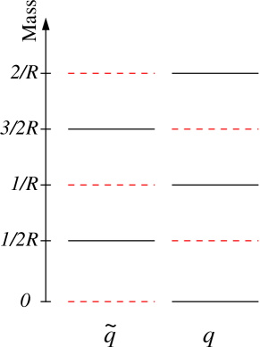
Figure 3: The Kaluza-Klein tower in theories with Scherk-Schwarz SUSY breaking admits non-degenerate fermions and bosons. However in folded-supersymmetric theory each such tower is complemented by another tower yielding a degenerate spectrum. This allows for a complete cancellation of radiative corrections to the Higgs mass at one loop.

III.2 SU(2) Gauge Interactions

Choice of Orbifold

We now consider how to cancel the dominant one loop quadratically divergent contributions to the Higgs mass from SU(2) gauge interactions. If we treat SU(2) indices $i$ as large $N$ indices, in t’Hooft double line notation the gauge contribution to the Higgs mass parameter takes the form shown in Figure (4).

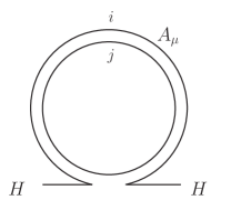
Figure 4: The gauge loop contribution to the Higgs mass in double line notation. In order to give the Higgs bifold protection SU(2) may be extended to SU(4).

From the diagram it is clear that it is SU(2) indices which are being summed over in the loop. Therefore, in order to obtain a theory where the Higgs mass enjoys bifold protection, we must supersymmetrize and double the sum over SU(2) indices. One way of doubling the sum is to extend the SM gauge structure from SU(3$)\times$ SU(2$)\times$ U(1) to SU(3$)\times$ SU(4$)\times$ U(1). The up and down-type Higgs fields, ${H}_{U}$ and ${H}_{D}$ then transform as $4$ and $\overline{4}$ under the SU(4) symmetry. The resulting theory possesses a $Z_{2\Gamma}$ symmetry under which ${H}_{U}\rightarrow\Gamma{H}_{U}$, ${H}_{D}\rightarrow\Gamma^{*}{H}_{D}$. Also $V_{4}\rightarrow\Gamma_{4}V_{4}\Gamma_{4}^{\dagger}$. As before the theory is invariant under a $Z_{2R}$ symmetry under which all bosonic fields are even and all fermionic fields odd. We now consider the transformation properties of the various fields under the combined $Z_{2\Gamma}\times Z_{2R}$ symmetry. For the components of the field $H_{U}$

$${h_{U}}=\pmatrix{h_{UA}(+)\cr h_{UB}(-)}\;\;\;\;\tilde{h}_{U}=\pmatrix{\tilde{h}_{UA}(-)\cr\tilde{h}_{UB}(+)}$$ (19)

For the components of $V_{4}$,

$$A_{\mu} = \pmatrix{A_{\mu,AA}(+)&A_{\mu,AB}(-)\cr A_{\mu,BA}(-)&A_{\mu,BB}(+)}$$

$$\lambda = \pmatrix{\lambda_{AA}(-)&\lambda_{AB}(+)\cr\lambda_{BA}(+)&\lambda_{BB}(-)}$$ (20)

Here $A$ and $B$ distinguish between the two SU(2) subgroups of SU(4). We now project out states odd under $Z_{2\Gamma}\times Z_{2R}$. The gauge symmetry is then broken down to SU(2$)\times$ SU(2$)\times$ U(1). Let us consider contributions from this sector to the mass of the Higgs scalar $h_{UA}$. Schematically, the relevant interactions are

$$\left|\left(\partial_{\mu}-igA_{\mu,AA}-i\frac{g}{\sqrt{2}}A_{\mu,D}\right)h_{UA}\right|^{2}+$$

$$\left[i\sqrt{2}g\;h_{UA}\lambda_{AB}\tilde{h}_{UB}+{\rm h.c.}\right]+\left[\;{\rm D-terms}\;\right]$$ (21)

where $A_{\mu,D}$ represents the gauge boson of the unbroken diagonal U(1). The SU(2) gauge interactions contribute $9/64\pi^{2}g^{2}\Lambda^{2}$ to the mass of $h_{UA}$, while from the scalar self-interactions that survive in the SU(2) D-term we obtain $3/64\pi^{2}g^{2}\Lambda^{2}$. The off-diagonal components of the SU(4) gauginos $\lambda_{AB}$ and $\lambda_{BA}$ contribute $-1/4\pi^{2}g^{2}\Lambda^{2}$, and finally $A_{\mu,D}$ and its D-term together contribute $1/32\pi^{2}g^{2}\Lambda^{2}$. The sum total is $-1/32\pi^{2}g^{2}\Lambda^{2}$, and so the cancellation is incomplete. This is because we started from SU(4) and not from U(4). Nevertheless, since the naive SM estimate of the contribution to the Higgs mass from SU(2) gauge loops is $9/64\pi^{2}g^{2}\Lambda^{2}$, this still represents an improvement over the SM by a factor of about 5 or so. However, the fact that the result is quadratically divergent means that whether this improvement is significant or not depends on whether a ultraviolet completion exists that is naturally consistent with this cancellation.

An Ultraviolet Completion

We now outline such an ultraviolet completion. As before we consider a five-dimensional supersymmetric theory with an extra dimension of radius $R$ compactified on $S^{1}/Z_{2}$, with branes at the orbifold fixed points. As before the branes are at $y=0$ and $y=\pi R$. The gauge symmetry is SU(3$)\times$ SU(4$)\times$ U(1), and all gauge fields live in the bulk of the higher dimensional space. This time it is the SU(4) gauge symmetry which is broken to SU(2$)\times$ SU(2$)\times$ U(1) by boundary conditions. As before supersymmetry is also broken by the Scherk-Schwarz mechanism, so that while physics on each brane respects a (different) four dimensional $\mathcal{N}=1$ supersymmetry, below the compactification scale supersymmetry is completely broken. The Higgs fields $H_{U}$ and $H_{D}$ are localized on the brane where SU(4) is preserved.

In order to break SU(4) to SU(2$)\times$ SU(2$)\times$ U(1) we must impose suitable boundary conditions. We choose $Z$ to leave SU(4) unbroken while $Z^{\prime}$ breaks SU(4). Then if we denote the five dimensional SU(4) gauge multiplet by $\hat{V}_{4}$, then under the action of $Z$, $V_{4}$ is even and $\Sigma_{4}$ odd. However, under the action of $Z^{\prime}$, $V^{\prime}_{4}\rightarrow\Gamma V^{\prime}_{4}\Gamma^{\dagger}$ while $\Sigma^{\prime}_{4}\rightarrow-\Gamma\Sigma^{\prime}_{4}\Gamma^{\dagger}$. Then the gauge bosons of SU(2$)\times$ SU(2$)\times$ U(1), together with the fields in $\lambda_{4}$ which have the quantum numbers of SU(4)/[SU(2) $\times$ SU(2) $\times$ U(1)], are the only ones with zero modes. If we now consider the couplings of the Higgs fields $H_{U}$ and $H_{D}$ to the zero modes of $\hat{V}_{4}$, they now have exactly the form of Eq. (III.2), with the remaining quadratic divergence from the U(1) cutoff by the Kaluza-Klein modes. The net contribution to the Higgs mass parameter in this theory is calculated in the appendix. It is non-zero but finite and about a factor of 20 smaller than the naive SM estimate of $9/64\pi^{2}g^{2}\Lambda^{2}$ when $\Lambda$ is replaced by $1/R$. Since we wish to leave SU(3$)\times$ U(1$)_{\rm Y}$ of the SM unbroken, for these vector multiplets we simply keep $V$ even under $Z$ and $V^{\prime}$ even under $Z^{\prime}$ while projecting out $\Sigma$ and $\Sigma^{\prime}$. Only the gauge bosons of SU(3$)\times$ U(1$)_{\rm Y}$ are then present in the low energy spectrum. It is possible to construct a completely realistic model along these lines but we leave this for future work.

IV A Realistic Model

We now construct a realistic model based on the tools we have developed in the last two sections. In this example, quadratically divergent contributions to the SM Higgs mass parameter from the SU(2) and U(1) gauge bosons are cancelled by the corresponding gauginos, just as in the MSSM. However, the one loop contributions to the Higgs mass from the top loop are cancelled by particles with no charge under SM color, giving rise to a very distinct and exciting phenomenology. The model is similar to the corresponding five dimensional model in section III.1. The major difference is that in this model the bulk SU(6) gauge symmetry is replaced by a bulk SU(3$)\times$ SU(3) gauge symmetry with a $Z_{2}$ interchange symmetry that links the particle content and coupling constants of the two SU(3) gauge interactions. The SU(3) $\times$ SU(3) $\times Z_{2}$ symmetry is sufficient to ensure that the Higgs mass parameter enjoys bifold protection from Yukawa interactions, which allows the crucial cancellation to go through just as in the SU(6) model.

Once again we begin with a five-dimensional supersymmetric theory. The extra dimension, which has radius $R$, is compactified on $S^{1}/Z_{2}$, and there are branes at the orbifold fixed points $y=0$ and $y=\pi R$. The gauge symmetry is now [SU(3$)_{A}\times$ SU(3$)_{B}]\times$ SU(2$)_{\rm L}\times$ U(1$)_{\rm Y}$, and as before all gauge fields live in the bulk of the higher dimensional space. While the SU(3$)_{A}$ gauge group corresponds to the familiar SM color, SU(3$)_{B}$ corresponds to a mirror color gauge group. The remaining SU(2$)_{\rm L}$ and U(1$)_{\rm Y}$ give rise to the SM weak and hypercharge interactions. All matter fields arise from hypermultiplets living in the five dimensional bulk. There is a discrete $Z_{2}$ symmetry in the bulk that interchanges the vector superfields of the two SU(3) gauge groups, but which acts trivially on SU(2$)_{\rm L}$ and U(1$)_{\rm Y}$ vector superfields. We label this interchange symmetry by $Z_{AB}$. The bulk hypermultiplets from which the SM quarks and their F-spartners emerge are

$$\hat{Q}_{iA}\;\;(3,1,2,{1}/{6}) \hat{Q}_{iB}\;\;(1,3,2,{1}/{6})$$

$$\hat{U}_{iA}\;\;(\bar{3},1,1,-{2}/{3}) \hat{U}_{iB}\;\;(1,\bar{3},1,-{2}/{3})$$

$$\hat{D}_{iA}\;\;(\bar{3},1,1,{1}/{3}) \hat{D}_{iB}\;\;(1,\bar{3},1,{1}/{3})$$ (22)

where the index $A$ denotes the SM fields and $B$ their F-partners. The index $i$, which runs from 1 to 3 labels the different SM generations. The numbers in brackets indicate the quantum numbers of the various fields under SU(3$)_{A}\times$ SU(3$)_{B}\times$ SU(2$)_{\rm L}\times$ U(1$)_{\rm Y}$. Under the bulk $Z_{AB}$ interchange symmetry the indices $A$ and $B$ are interchanged. The SM leptons and their F-spartners emerge from the bulk hypermultiplets below.

$$\hat{L}_{iA}\;\;(1,1,2,-{1}/{2}) \hat{L}_{iB}\;\;(1,1,2,-{1}/{2})$$

$$\hat{E}_{iA}\;\;(1,1,1,1) \hat{E}_{iB}\;\;(1,1,1,1)$$ (23)

Note that $\hat{L}_{iA}$ and $\hat{L}_{iB}$ have exactly the same gauge charges, as do $\hat{E}_{iA}$ and $\hat{E}_{iB}$. Once again, under the bulk $Z_{AB}$ interchange symmetry the indices $A$ and $B$ are interchanged. The boundary conditions on the bulk hypermultiplets are chosen to break both supersymmetry and the discrete $Z_{AB}$ symmetry. Specifically, we choose boundary conditions so that only the SM fields and their F-spartners are light.

• Of the fields $\hat{Q}_{iA}$, $\hat{U}_{iA}$, $\hat{D}_{iA}$, $\hat{L}_{iA}$ and $\hat{E}_{iA}$ only the fermions have zero modes, and

• of the fields $\hat{Q}_{iB}$, $\hat{U}_{iB}$, $\hat{D}_{iB}$, $\hat{L}_{iB}$ and $\hat{E}_{iB}$ only the bosons have zero modes.

This is realized in the following way. When written in terms of $\mathcal{N}=1$ superfields $\hat{Q}_{iA}$ can be decomposed into $(Q_{iA},Q_{iA}^{c})$ or into $(Q^{\prime}_{iA},Q_{iA}^{\prime c})$. Under the action of $Z$, $Q_{iA}$ is even while $Q_{iA}^{c}$ is odd and under the action of $Z^{\prime}$, $Q^{\prime}_{iA}$ is even while $Q_{iA}^{\prime c}$ is odd. These boundary conditions project out a zero mode fermion but no corresponding light scalar. Zero mode fermions can be obtained from $\hat{U}_{iA},\hat{D}_{iA},\hat{L}_{iA}$ and $\hat{E}_{iA}$ by applying exactly the same boundary conditions.

What about the mirror fields? When written in terms of $\mathcal{N}=1$ superfields $\hat{Q}_{iB}$ can be decomposed into $(Q_{iB},Q_{iB}^{c})$ or into $(Q^{\prime}_{iB},Q_{iB}^{\prime c})$. Under the action of $Z$, $Q_{iB}$ is even while $Q_{iB}^{c}$ is odd, and under the action of $Z^{\prime}$, $Q^{\prime}_{iB}$ is odd while $Q_{iB}^{\prime c}$ is even. These boundary conditions project out a zero mode scalar but no corresponding light fermion. Zero mode scalars can be obtained from $\hat{U}_{iB}$, $\hat{D}_{iB}$, $\hat{L}_{iB}$ and $\hat{E}_{iB}$ by applying exactly the same boundary conditions. Note that the symmetry $Z_{AB}$ is broken by the boundary conditions at $y=\pi R$, but not at $y=0$. This choice of brane and bulk fields implies the absence of mixed U(1) and gravitational anomalies anywhere in the space. Then Fayet-Iliapoulos terms are not radiatively generated at the boundaries FIterms1 ; FIterms2 .

The MSSM Higgs fields are localized on the brane at $y=0$. We extend the $Z_{2}$ interchange symmetry of the bulk to this brane. Then the Higgs couples with equal strength to both SM fields and mirror fields, and the top Yukawa coupling has the form

$$W=\delta\left(y\right)\lambda_{t}\left[Q_{3A}H_{U}U_{3A}+Q_{3B}H_{U}U_{3B}\right]$$ (24)

Notice that the SU(3) $\times$ SU(3) $\times Z_{2}$ symmetry tightly constrains the form of the top Yukawa coupling. In particular, this interaction takes exactly the same SU(6) symmetric form as in the corresponding theory in the previous section. This ensures that the Higgs mass parameter enjoys bifold protection from radiative corrections arising from the top Yukawa. The interactions of the Higgs in the four dimensional effective theory again have the folded-supersymmetric form of Eq (III.1). As before, the one-loop contribution to the Higgs mass parameter from the top loop is cancelled by the mirror stops. As shown in the appendix this cancellation is not restricted to the zero-modes but persists all the way up the Kaluza-Klein tower and is guaranteed by a combination of supersymmetry and the discrete symmetry. Therefore the top Yukawa coupling does not contribute to the Higgs mass at one loop.

In this theory the top Yukawa coupling, which is required to be of order one, is volume suppressed. This implies that the cutoff $\Lambda$ of this theory cannot be much larger than inverse of the compactification scale, $\Lambda\mathrel{\mathchoice{\vereq\displaystyle{<}}{\vereq\textstyle{<}}{\vereq\scriptstyle{<}}{\vereq\scriptscriptstyle{<}}}4R^{-1}$. This leads to a potential problem. Kinetic terms of the form $\int d^{4}\theta\;Q_{3\alpha}^{{}^{\prime}\dagger}e^{V}Q^{\prime}_{3\alpha}$ localized on the brane at $y=\pi R$ which do not respect the $Z_{AB}$ symmetry may affect the cancellation. However, this difficulty can be avoided by imposing an additional symmetry on the theory. In the bulk the theory possesses a discrete charge conjugation symmetry under which the SM matter fields are interchanged with their corresponding charge conjugate fields in the mirror sector. This takes the form

$$Q_{iA}^{\prime}\leftrightarrow Q_{iB}^{\prime c} Q_{iB}^{\prime}\leftrightarrow-Q_{iA}^{\prime c}$$

$$U_{iA}^{\prime}\leftrightarrow U_{iB}^{\prime c} U_{iB}^{\prime}\leftrightarrow-U_{iA}^{\prime c}$$

$$D_{iA}^{\prime}\leftrightarrow D_{iB}^{\prime c} D_{iB}^{\prime}\leftrightarrow-D_{iA}^{\prime c}$$

$$L_{iA}^{\prime}\leftrightarrow L_{iB}^{\prime c} L_{iB}^{\prime}\leftrightarrow-L_{iA}^{\prime c}$$

$$E_{iA}^{\prime}\leftrightarrow E_{iB}^{\prime c} E_{iB}^{\prime}\leftrightarrow-E_{iA}^{\prime c}$$ (25)

The vector superfields of SM color are also to be interchanged with their charge conjugates in the the mirror color sector while the vector superfields of SU(2$)_{\rm L}$ and U(1$)_{\rm Y}$ simply transform into their charge conjugates. We label this discrete symmetry by $Z^{\prime}_{AB}$. Although the boundary conditions break this discrete symmetry on the brane at $y=0$, this symmetry can be consistently extended to the brane at $y=\pi R$. This provides a restriction on the form of the brane-localized kinetic terms at $y=\pi R$ so that the cancellation of all one loop corrections to the Higgs mass parameter from the top sector continues to hold.

The zero-mode F-spartners will acquire masses radiatively, primarily from gauge interactions. The masses of these fields have been calculated in APQ .

$$m_{Q}^{2} = {\rm K}\;\frac{1}{4\pi^{4}}\left(\frac{4}{3}g_{3}^{2}+\frac{3}{4}g_{2}^{2}+\frac{1}{36}g_{1}^{2}\right)\frac{1}{R^{2}}$$

$$m_{U}^{2} = {\rm K}\;\frac{1}{4\pi^{4}}\left(\frac{4}{3}g_{3}^{2}+\frac{4}{9}g_{1}^{2}\right)\frac{1}{R^{2}}$$

$$m_{D}^{2} = {\rm K}\;\frac{1}{4\pi^{4}}\left(\frac{4}{3}g_{3}^{2}+\frac{1}{9}g_{1}^{2}\right)\frac{1}{R^{2}}$$

$$m_{L}^{2} = {\rm K}\;\frac{1}{4\pi^{4}}\left(\frac{3}{4}g_{2}^{2}+\frac{1}{4}g_{1}^{2}\right)\frac{1}{R^{2}}$$

$$m_{E}^{2} = {\rm K}\;\frac{1}{4\pi^{4}}g_{1}^{2}\frac{1}{R^{2}}$$ (26)

Here K is a dimensionless constant whose numerical value is close to 2.1, while $g_{3}$, $g_{2}$ and $g_{1}$ are the gauge coupling constants of SU(3$)$, SU(2$)_{\rm L}$ and U(1$)_{\rm Y/2}$ respectively. Here we have neglected contributions to the masses of the F-spartners from their Yukawa couplings to the Higgs, which are negligible except for the third generation F-stops. As shown in the appendix, for these fields we need to add

$$m_{Q}^{2}={\rm K}\;\frac{\lambda_{t}^{2}}{8\pi^{4}}\frac{1}{R^{2}}\,,\qquad m_{U}^{2}={\rm K}\;\frac{\lambda_{t}^{2}}{4\pi^{4}}\frac{1}{R^{2}}\,.$$ (27)

The only F-partners with masses less than 50 GeV are the gluons of mirror color. These will confine into F-glueballs at a scale $\Lambda_{\rm F-QCD}$ of order a few GeV. Since these couple only very weakly to the SM particles at low energies, they evade current experimental bounds.

In this theory where do the leading contributions to the Higgs potential come from? As shown in the appendix gauge interactions give rise to a finite and positive one loop contribution to the mass parameters of both the up-type and down-type Higgs that takes the form

$$\delta m_{H}^{2}|_{\rm gauge}={\rm K}\;\frac{3g_{2}^{2}+g_{1}^{2}}{16\pi^{4}}\frac{1}{R^{2}}$$ (28)

However, at two loops there is a finite negative contribution to the mass of the up-type Higgs from the top sector of order

$$\delta m_{H}^{2}|_{\rm top}\approx-\frac{3\lambda_{t}^{2}}{4\pi^{2}}\tilde{m}_{t}^{2}\;{\rm log}\left(\frac{1}{R\;\tilde{m}_{t}}\right)$$ (29)

where $\tilde{m}_{t}$ is the mass of the F-stop. A quick estimate suggests that the top contribution is larger in magnitude than the gauge contribution from Eq.(28), leading to electroweak symmetry breaking. However, to be certain of this a more careful analysis is required, which we leave for future work.

At this stage the tree-level Higgs quartic in our model is identical to that of the MSSM, and is therefore too small to give rise to a Higgs mass larger than the current experimental lower bound of 114 GeV. We therefore extend the Higgs sector by adding to the theory an extra singlet $S$ which is localized to the brane at $y=0$ and couples to the Higgs as

$$\delta\left(y\right)\int d^{2}\theta\left[\alpha S+\lambda SH_{u}H_{d}+\kappa S^{3}\right]$$ (30)

For ${\rm tan}\beta$ close to one and values of $\lambda$ greater than about 0.65 this will give rise to tree level Higgs masses greater than the experimental lower bound. Since the cutoff $\Lambda$ of the theory is low, it is not difficult to generate a value for $\lambda$ larger than this TW . In the absence of the linear term in the superpotential the Higgs potential has an exact U(1$)_{\rm R}$ symmetry. The term $\alpha S$ breaks this continuous symmetry in the softest possible way leaving behind only a discrete $Z_{4}$ R symmetry. This suffices to ensure the absence of an unwanted Goldstone boson. We choose the value of $\alpha$ to be of order weak scale size to obtain consistent electroweak breaking. This choice is technically natural. We leave the problem of naturally generating $\alpha$ of this size for future work.

The VEV of the singlet $S$ serves as an effective $\mu$ term. A negative mass for the scalar in $S$ can be generated by introducing into the bulk two SM singlet hypermultiplets $\hat{P}_{A}$ and $\hat{P}_{B}$. The boundary conditions on these fields are such as to allow only a fermion zero mode for each of $\hat{P}_{A}$ and $\hat{P}_{B}$. The bulk $Z_{AB}$ symmetry interchanges $\hat{P}_{A}$ and $\hat{{P}}_{B}$. In addition, under the $Z_{AB}^{\prime}$ symmetry, $\hat{P}_{A}$ and $\hat{{P}}_{B}$ are also interchanged. Then on the brane at $y=0$ we can write the interaction

$$\delta\left(y\right)\int d^{2}\theta\left[\lambda_{P}SP_{A}P_{B}+\mu_{P}\left({P_{A}}^{2}+{P_{B}}^{2}\right)\right]$$ (31)

The effect of the coupling $\lambda_{P}$ is to generate a negative mass squared for the scalar in $S$ at one loop. The theory is also invariant under a discrete symmetry, pedestrian parity pedestrian , under which $\hat{P}_{A}$ and $\hat{{P}}_{B}$ change sign but all other fields are invariant. Pedestrian parity ensures that the zero-mode fermions in $\hat{P}_{A}$ and $\hat{P}_{B}$ are stable. These particles are potential dark matter candidates.

We are now in a position to understand the extent to which this model addresses the LEP paradox. Since the largest contribution to the Higgs mass arises from the top sector, and assuming the lightest neutral Higgs is SM-like and the other Higgs fields are significantly heavier, we can estimate the fine-tuning by the formula

$$\frac{m_{H,{\rm phys}}^{2}}{2\delta m_{H}^{2}|_{\rm top}}\times 100\%$$ (32)

Here $m_{H,{\rm phys}}$ is the physical mass of the lightest neutral Higgs, and $\delta m_{H}^{2}|_{\rm top}$ is to be calculated from Eq.(29). For a compactification scale $1/R$ of order 5 TeV, a cutoff $\Lambda$ of order 20 TeV and $m_{H,{\rm phys}}=115$ GeV the fine-tuning is about $12\%$. The fine-tuning decreases for larger values of $m_{H,{\rm phys}}$ and falls to about $40\%$ for $m_{H,{\rm phys}}=200$ GeV. For comparison, the SM with a cutoff of 20 TeV is fine tuned at the $0.1\%$ level for $m_{H,{\rm phys}}=200$ GeV. A complete solution to the hierarchy problem may be obtained if there is a warped extra dimension RS in addition to the compact fifth dimension. Models of this type have been constructed in CN99 .

In the absence of further interactions between the $A$ and $B$ sectors the lightest F-spartner, which is right-handed F-slepton, is absolutely stable and does not decay. In order to avoid the cosmological bounds on stable charged particles we add to the theory the non-renormalizable interactions

$$\delta\left(y\right)\int d^{2}\theta\left(\frac{Q_{A}Q_{A}Q_{A}L_{B}}{\Lambda}+\frac{Q_{B}Q_{B}Q_{B}L_{A}}{\Lambda}\right)$$ (33)

and

$$\delta\left(y\right)\int d^{2}\theta\left(\frac{U_{A}U_{A}D_{A}E_{B}}{\Lambda}+\frac{U_{B}U_{B}D_{B}E_{A}}{\Lambda}\right)$$ (34)

where we have suppressed the indices labeling the different generations. An F-slepton can then decay to three quarks and the LSP, which in this model is mostly Higgsino or singlino. F-baryons are also no longer stable, and decay before nucleosynthesis. The SM baryons, however, are still stable because decays to F-sleptons or F-leptons are kinematically forbidden. Although the interactions in Eq. (33) and Eq. (34) give rise to flavor violating effects, these are small and consistent with current bounds. Precision electroweak constraints on this model are satisfied, as shown in the appendix.

What are the characteristic collider signatures of this theory? The F-sleptons can be pair produced at the LHC through their couplings to the W,Z and photon. Each F-slepton decays to three quarks and the LSP. The high dimensionality of the relevant effective operator implies that for reasonable values of the couplings the F-slepton may travel anywhere from a few millimeters to tens of meters before decaying. The collider signatures are therefore expected to consist of either six jet events with displaced vertices, or highly ionizing tracks corresponding to massive stable charged particles.

For the F-squarks the situation is rather different. While they can also be pair produced in colliders through their couplings to the W,Z and photon they are charged under F-color rather than SM color. Then the absence of light states with charge under F-color other than F-gluons prevents the F-squarks from hadronizing individually. They therefore behave like scalar quirks Matt1 ; LKN , or ‘squirks’. The two F-squarks are connected by an F-QCD string and together form a bound state. This bound state system is initially in a very excited state but we expect that it will quickly cascade down to a lower energy state by the emission of soft F-glueballs and photons. Eventually the two F-squarks pair-annihilate into two (or more) hard F-glueballs, two hard W’s, two hard Z’s or two hard photons. They could also pair-annihilate through a single off-shell W,Z or photon into two hard leptons or jets. The decay of the bound state is prompt on collider time scales.

Before we can understand the collider signatures associated with the production of squirks, we must first estimate the F-glueball lifetime. Below the mass scale of the F-squarks this is essentially a ‘hidden valley’ model Matt1 ; Matt2 . The F-glueball must decay back to SM states because decays to F-(s)partners are kinematically forbidden. The dominant decays occur through an off-shell Higgs and the decay products are charm quarks and tau leptons, and perhaps bottom quarks as well if the F-glueball is sufficiently heavy. The coupling of the Higgs to the F-glueball is through a loop of virtual F-stops. The high dimensionality of this operator implies that F-glueballs are stable on collider time scales and almost all escape the detector. A naive estimate of the range yields about 10 Km., but this answer is very sensitive to the exact values of $\Lambda_{\rm F-QCD}$ and the F-glueball mass. As a consequence, it is conceivable that the range is as much as a factor of a thousand smaller than this, which would be very exciting from the collider viewpoint. Nevertheless, in what follows, we shall trust our naive estimate of the lifetime and assume that F-glueballs escape the detector.

The characteristic signatures of this scenario therefore include (but are not limited to) events with

• four hard leptons (from the two Z’s) accompanied by missing energy,

• two hard leptons (from the two W’s, or from the off-shell Z or photon) accompanied by missing energy, and

• two hard photons accompanied by missing energy

It should be possible to determine the masses of the F-squarks from the energy distributions of the outgoing leptons. These signatures are very distinctive, and, if there are enough events, should make this model relatively straightforward to distinguish at the LHC. In addition to this, it may be possible to detect the characteristic experimental signatures of TeV size extra dimensions, such as Kaluza-Klein resonances and deviations from Newtonian gravity at sub-millimeter distances submm . The cosmology of theories with a TeV size extra dimension has been considered, for example, in cosmo .

Neutrino masses in this model may be either Dirac or Majorana. Since Majorana neutrino masses violate lepton number by two units, the $A\rightarrow B$ symmetry together with Eqns. (33) and (34) imply that in this case the model predicts neutron-antineutron oscillations. However, since the amplitude for this process is proportional to the small neutrino masses, the rates for this are completely consistent with the current experimental bounds nnbar .

V Conclusions

In summary, we have constructed a new class of theories which address the LEP paradox. These ‘folded supersymmetric’ theories predict a rich spectrum of new particles at the TeV scale which may be accessible to upcoming experiments. Together with mirror symmetric twin Higgs models, these theories are explicit counterexamples to the conventional wisdom that canceling the one-loop quadratic divergences to the Higgs mass parameter from the top sector necessarily requires new particles charged under SM color.

Acknowledgments –
We thank E. Cheu, M. Luty, T. Okui, M. Strassler and E. Varnes for discussions. G.B. acknowledges the support of the State of São Paulo Research Foundation (FAPESP), and of the Brazilian National Counsel for Technological and Scientific Development (CNPq). Z.C and H.S.G are supported by the NSF under grant PHY-0408954. R.H. is supported by the US Department of Energy under Contract No. DE-AC02-76SF00515.

Appendix A Radiative Corrections in Higher Dimensions

A.1 The SU(3) $\times$ SU(3) Model

In this appendix we will determine the radiative corrections to the Higgs mass in five dimensional folded-supersymmetric models. The corrections are finite and depend on the the supersymmetric structure of the higher dimensional theory as well as other global or gauge symmetries, depending on the specific model. We first focus on the realistic SU(3) $\times$ SU(3) model of section IV. We shall see that the cancellation of one loop quadratic divergences is a consequence of supersymmetry and the discrete $Z_{2}$ symmetry $Z_{AB}$. We note that the calculation for the SU(6) model of section III.1 is identical to the one outlined below.

The one loop effective potential for the Higgs has the convenient property that different interactions of the Higgs contribute additively. Therefore, when calculating the contribution to the potential from, say, the top Yukawa, one can ignore the gauge interaction of the Higgs and vice versa. Following PeskinMirabelli ; Jay5Dsusy we write the part of the higher dimensional Lagrangian which is relevant for the cancellation of one loop quadratic divergences from the top sector in terms of $\mathcal{N}=1$ superfields. Even though the bulk Lagrangian possesses an SU(2$)_{R}$ symmetry, it is convenient to write the higher dimensional Lagrangian in the SU(2$)_{R}$ basis that is aligned with the unbroken $\mathcal{N}=1$ supersymmetry on the Higgs brane.

$$\mathcal{L}_{5D} = \int d^{4}\theta\left[Q_{A}^{\dagger}Q_{A}+Q_{A}^{c\dagger}Q^{c}_{A}+U_{A}^{\dagger}U_{A}+U_{A}^{c\dagger}U^{c}_{A}+Q_{B}^{\dagger}Q_{B}+Q_{B}^{c\dagger}Q^{c}_{B}+U_{B}^{\dagger}U_{B}+U_{B}^{c\dagger}U^{c}_{B}\right]$$ (35)

$$+ \int d^{2}\theta\left[Q_{A}^{c}\partial_{5}Q_{A}+U_{A}^{c}\partial_{5}U_{A}+Q_{B}^{c}\partial_{5}Q_{B}+U_{B}^{c}\partial_{5}U_{B}\right]+\mbox{h.c.}$$

$$+ \delta(y)\left\{\int d^{4}\theta H_{u}^{\dagger}H_{u}+\int d^{2}\theta\left[\lambda_{t}H_{u}Q_{A}U_{A}+\lambda_{t}H_{u}Q_{B}U_{B}\ \right]+\mbox{h.c}\right\}$$

Here, and for the rest of this appendix, we have suppressed the label ‘3’ denoting the third generation for simplicity. We have also neglected possible brane kinetic terms which we will come back to later.

It is straightforward to decompose the bulk fields into Kaluza-Klein modes according to their various boundary conditions. Zero modes exist only for the $(+,+)$ fields, the fermion components of $Q_{A}$ and $U_{A}$ as well as the scalar components of $Q_{B}$ and $U_{B}$. The relevant part of the Lagrangian for the zero mode fields alone, in components, is

$$\mathcal{L}_{(0)} = \mbox{kinetic terms}+\lambda_{t}H_{u}q_{A0}u_{A0}+\mbox{h.c.}$$ (36)

$$+ \lambda_{t}^{2}|H_{u}|^{2}|\tilde{q}_{B0}|^{2}+\lambda_{t}^{2}|H_{u}|^{2}|\tilde{u}_{B0}|^{2}\,.$$

Notice that this part of the Lagrangian has an accidental supersymmetry. In particular, if we switch all labels, $A\leftrightarrow B$, on scalar fields only, it appears to have an exactly supersymmetric structure. Furthermore, the higher-dimensional supersymmetry together with the $Z_{AB}$ interchange guarantees that a regulator exists which preserves this accidentally supersymmetric structure of the zero-mode Lagrangian. (Metaphorically, the cutoffs of the fermion and scalar sectors are identical). This demonstrates that the extra-dimensional theory is indeed an ultraviolet completion for the 4D folded supersymmetric model. The one loop contribution of the zero mode top sector to the Higgs mass vanishes.

Now let us turn our attention to the part of the Lagrangian involving Kaluza-Klein modes which is relevant for the cancellation of one loop quadratic divergences from the top sector.

$$\mathcal{L}^{(KK)} = \sum_{n}\left[\mbox{kinetic terms}\right]$$ (37)

$$+ \sum_{n}\left[\frac{n}{R}q_{An}^{c}q_{An}+\frac{n}{R}u_{An}^{c}u_{An}+\left(\frac{2n+1}{2R}\right)^{2}|\tilde{q}_{An}|^{2}+\left(\frac{2n+1}{2R}\right)^{2}|\tilde{q}^{c}_{An}|^{2}+\left(\frac{2n+1}{2R}\right)^{2}|\tilde{u}_{An}|^{2}+\left(\frac{2n+1}{2R}\right)^{2}|\tilde{u}^{c}_{An}|^{2}\right.$$

$$\qquad+\left.\frac{2n+1}{2R}q_{Bn}^{c}q_{Bn}+\frac{2n+1}{2R}u_{Bn}^{c}u_{Bn}+\left(\frac{n}{R}\right)^{2}|\tilde{q}_{Bn}|^{2}+\left(\frac{n}{R}\right)^{2}|\tilde{q}^{c}_{Bn}|^{2}+\left(\frac{n}{R}\right)^{2}|\tilde{u}_{Bn}|^{2}+\left(\frac{n}{R}\right)^{2}|\tilde{u}^{c}_{Bn}|^{2}\right]$$

$$+ \sum_{n,m}\left[\lambda_{t}H_{u}q_{Bn}u_{Bm}+\lambda_{t}^{2}|H_{u}|^{2}|\tilde{q}_{An}|^{2}+\lambda_{t}^{2}|H_{u}|^{2}|\tilde{u}_{Am}|^{2}+\lambda_{t}\frac{2m+1}{2R}H_{u}\tilde{q}_{An}\tilde{u}^{c*}_{Am}+\lambda_{t}\frac{2n+1}{2R}H_{u}\tilde{q}^{c*}_{An}\tilde{u}_{Am}\right.$$

$$\ \ \ +\left.\lambda_{t}H_{u}q_{An}u_{Am}+\lambda_{t}^{2}|H_{u}|^{2}|\tilde{q}_{Bn}|^{2}+\lambda_{t}^{2}|H_{u}|^{2}|\tilde{u}_{Bm}|^{2}+\lambda_{t}\frac{m}{R}H_{u}\tilde{q}_{Bn}\tilde{u}^{c*}_{Bm}+\lambda_{t}\frac{n}{R}H_{u}\tilde{q}^{c*}_{Bn}\tilde{u}_{Bm}\right]$$

$$+ \sum_{n}\left[\lambda_{t}H_{u}q_{An}u_{A0}+\lambda_{t}^{2}|H_{u}|^{2}|\tilde{q}_{Bn}|^{2}+\lambda_{t}^{2}|H_{u}|^{2}|\tilde{u}_{B0}|^{2}+\lambda_{t}\frac{n}{R}H_{u}\tilde{q}^{c*}_{Bn}\tilde{u}_{B0}\right]$$

$$+ \sum_{m}\left[\lambda_{t}H_{u}q_{A0}u_{Am}+\lambda_{t}^{2}|H_{u}|^{2}|\tilde{q}_{B0}|^{2}+\lambda_{t}^{2}|H_{u}|^{2}|\tilde{u}_{Bm}|^{2}+\lambda_{t}\frac{m}{R}H_{u}\tilde{q}_{B0}\tilde{u}^{c*}_{Bm}\right]\,.$$

Here the sums over the Kaluza-Klein indices $n$ and $m$ begin at one. The cancellation of the one loop contribution to the Higgs mass will be apparent once we familiarize ourselves with equation (37). The first term in brackets following the kinetic terms contains mass terms for the Kaluza-Klein fields. The second term in brackets, with summation over both $n$ and $m$, is the set of interactions between the Higgs and Kaluza-Klein modes. The last two terms in brackets are interactions between the Higgs, a zero mode and a single Kaluza-Klein mode. The interactions have been grouped such that every line in (37) involves degenerate fermions and scalars. For example, the second term in brackets involves the fermions $q_{An}$ and $u_{Am}$ with masses $n/R$ and $m/R$ respectively. The same term involves the scalars $\tilde{q}_{Bn}$, $\tilde{q}^{c}_{Bn}$ with mass $n/R$ and the scalars $\tilde{u}_{Bm}$, $\tilde{u}_{Bm}^{c}$ with mass $m/R$. Furthermore, the structure of the interactions within each term in brackets is formally identical to that of a supersymmetric theory. Specifically, if as before we switch all labels, $A\leftrightarrow B$, on scalar fields only, the relevant part of the Lagrangian appears to have an exactly supersymmetric structure. Note however that this relabeling is not a symmetry of the full Lagrangian, once one takes into account the gauge interactions. The Higgs is “fooled” into living in an exactly supersymmetric theory but only at one loop. The diagrams responsible for the cancellation are shown in Figure (5).

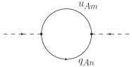
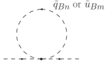
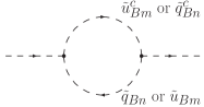
Figure 5: The Feynman diagrams involved in the cancellation of the radiative corrections to the Higgs mass from the top sector. For every choice of two Kaluza-Klein levels $n$ and $m$ this combination of diagrams is present, adding up to zero. The cancellation has a supersymmetric form, but the scalar tops are not charged under SM color.

In addition to the terms in equation (35) the Lagrangian may contain brane kinetic terms for the bulk fields. These break the bulk supersymmetry but preserve the appropriate 4D $\mathcal{N}=1$ supersymmetry on each brane. These terms can only be written for fields that are even around each fixed point, e.g. $Q$ at $y=0$ and $Q^{\prime}$ at $y=\pi R$. However, by writing these brane kinetic terms explicitly one can verify that the accidental supersymmetry of the relevant part of the Lagrangian is preserved so long as the brane kinetic terms respect the unbroken $Z_{2}$ at each brane. We therefore require that the Lagrangians on the branes respect $Z_{AB}$ at $y=0$ and $Z_{AB}^{\prime}$ at $y=\pi R$.

The exact cancellation of the one-loop Higgs mass in this model occurs only in the top sector. However, due to the non-local breaking of supersymmetry, the SU(2) gauge boson contribution is completely finite. To calculate this contribution we closely follow the approach of APQ . We are interested in the one loop Coleman-Weinberg (CW) effective potential CW due to gauge bosons, gauginos, as well as the chiral part of the $\mathcal{N}=2$ vector multiplet, running in loops. The CW potential is determined by calculating the one loop vacuum energy in terms of the field dependent masses. The CW potential from a Kaluza-Klein tower has the form

$$V(H)=\frac{1}{2}\mbox{Tr}\int\frac{d^{4}k}{(2\pi)^{4}}\sum_{n=-\infty}^{n=\infty}\ln\left(\frac{k^{2}+M^{2}_{Bn}+M^{2}(H)}{k^{2}+M^{2}_{Fn}+M^{2}(H)}\right)$$ (38)

where $M^{2}_{Bn}$ and $M^{2}_{Fn}$ are the $n$th boson and fermion Kaluza-Klein mass respectively, and $M(H)^{2}$ is the field dependent part of the mass which is common for both bosons and fermions due to supersymmetry. Since we are only interested in the mass, we can focus on the coefficient of $|H|^{2}$

$$m^{2}_{H}= \frac{dM^{2}(H)}{d|H|^{2}}$$ Tr

$$\times \int\frac{d^{4}k}{(2\pi)^{4}}\sum_{n=-\infty}^{n=\infty}\left[\frac{1}{k^{2}+M^{2}_{Bn}}-\frac{1}{k^{2}+M^{2}_{Fn}}\right]$$

In our case, the fermions, whose boundary conditions are $(+,-)$ and $(-,+)$, have Kaluza-Klein masses of $(2n+1)/2R$. The bosons, with boundary conditions of $(+,+)$ and $(-,-)$ have Kaluza-Klein masses of $n/R$. However, the trace in equation (A.1) runs only over $(+,+)$ and $(+,-)$ since only those couple to the Higgs brane. The sum over Kaluza-Klein modes is performed before integrating over phase space. One should note that the couplings of the Higgs to the Kaluza-Klein gauge bosons and gauginos is not diagonal in the Kaluza-Klein basis because the Higgs is localized to the brane. However, these off diagonal gauge interactions do not contribute to the Higgs mass at one loop, simplifying the calculation significantly. The final result is for the one-loop contribution to the Higgs mass from SU(2) gauge bosons is

$$\delta m^{2}_{H}|_{\mathrm{gauge}}={7C(H)\zeta(3)}\frac{g^{2}}{16\pi^{4}R^{4}}$$ (40)

where $C(H)$ is the quadratic Casimir. Identifying $K\equiv 7\zeta(3)/4\sim 2.1$ gives the one loop mass of equation (28). Finally, one can perform a similar calculation for the Yukawa contribution to the mirror stop masses (again neglecting off diagonal elements in the stop dependent mass matrix). This yields the stop mass contributions of equations (26) and (27).

A.2 The SU(4) Model

We now turn to the SU(4) model of section III.2. In this model the quadratic divergence that comes from loops of gauge boson zero modes is partially cancelled by loops of the zero modes of the off-diagonal gaugino bi-doublets. In the full extra dimensional theory the remaining quadratic divergence is cutoff at the scale $1/R$ because of the non-local nature of supersymmetry breaking in Scherk-Schwarz theories. In other words, when the sum over the entire Kaluza-Klein tower is added to the contribution of the zero mode to the Higgs mass, we get finite results. The extent of the cancellation between the boson Kaluza-Klein tower and the fermion Kaluza-Klein tower can be understood from the relevant group theory factors. The group theory factor $\sum_{a}T^{a}T^{a}$ coming from the diagrams involving the diagonal block is +7/8 (which is 3/4 from the SU(2) plus 1/8 from the diagonal generator of SU(4)). The off-diagonal bi-doublets contribute a factor of $-1$ (the sign is opposite because the spin of the particles in this tower is opposite). The left over contribution thus has a coefficient of $-1/8$. Note that the residual factor of $1/8$ would be cancelled exactly by the additional diagonal gauge boson in the case where the full U(4) is gauged, as expected.

It is straightforward to explicitly sum the Kaluza-Klein towers using the methods of  APQ . The gauge contribution to the Higgs mass squared in this model is then

$$m^{2}_{h}|_{\rm gauge}=-{\rm K}\frac{g_{2}^{2}}{32\pi^{4}}\frac{1}{R^{2}}.$$ (41)

This is about a factor of 20 smaller than the naive SU(2) gauge contribution to the Higgs mass squared in the SM,

$$m^{2}_{h}|_{\rm gauge,SM}\approx\frac{9g_{2}^{2}}{64\pi^{2}}\Lambda^{2}$$ (42)

when cut-off at the scale $\Lambda=1/R$.

Appendix B Electroweak Precision Constraints

Electroweak precision measurements tightly constrain the couplings of SM matter. The F-(s)partners and superpartners only contribute to these processes through loops, and therefore give only subdominant contributions. Thus for the most part, the theory we consider is the SM in a five dimensional bulk, with the Higgs localized at $y=0$. In this theory Kaluza-Klein number is conserved in the bulk uedbounds . Violation of Kaluza-Klein number is induced by brane-localized operators, which are volume suppressed. As a consequence, the exchange of gauge Kaluza-Klein modes does not lead to new, unsuppressed, four-fermion operators of the zero-mode fermions. The volume suppression in these four-fermion operators renders their effects harmless.

Nevertheless, there remain several sources of deviations from the SM values. The main constraint on the compactification scale $R$ will come from the tree-level mixing between the gauge boson zero modes and the their Kaluza-Klein excitations. This is induced by the presence of the localized Higgs vacuum expectation value $v$, and results in tree-level contributions to the electroweak parameters $S$, $T$ and $U$.

In order to compute the electroweak constraint, we assume the limit in which the light Higgs couples very nearly as the SM Higgs. The Higgs is localized on the brane at $y=0$. We are interested in the gauge sector, including the scalar kinetic term. The relevant terms in the action are

$$S_{5D} = \int d^{4}x\int_{0}^{\pi R}dy\left\{-\frac{1}{4}W_{MN}^{a}W^{aMN}-\frac{1}{4}B_{MN}B^{MN}\right.$$ (43)

$$\left.+\delta(y)\left(D_{\mu}\Phi\right)^{\dagger}D^{\mu}\Phi+\cdots\right\}$$

where $\Phi$ is the localized Higgs doublet and the covariant derivative is

$$D_{\mu}\Phi=\left(\partial_{\mu}-ig_{5}W_{\mu}^{a}t^{a}-ig^{\prime}_{5}\frac{1}{2}B_{\mu}\right)\Phi~{}.$$ (44)

The expansion in Kaluza-Klein modes for $B_{\mu}(x,y)$ can be written as

$$B_{\mu}(x,y)=\frac{1}{\sqrt{\pi R}}\left\{B_{\mu}^{(0)}(x)+\sqrt{2}\sum_{n=1}B_{\mu}^{(n)}(x)\cos\left(\frac{ny}{R}\right)\right\}~{},$$ (45)

and similarly for the $W_{\mu}^{a}$ fields. We work in the $W_{5}^{a}=B_{5}=0$ gauge.

The vacuum expectation value of the Higgs

$$\langle\Phi\rangle=\left(\begin{array}[]{c}0\\ \frac{v}{\sqrt{2}}\end{array}\right)$$ (46)

results in the localized action

$$S_{5D}^{\rm local.} = \int d^{4}x\int_{0}^{\pi R}dy\delta(y)\frac{v^{2}}{4}\left\{g_{5}^{2}W_{\mu}^{-}W^{\mu+}\right.$$ (47)

$$\left.+\frac{1}{2}(g_{5}^{2}+g_{5}^{{}^{\prime}2})Z_{\mu}Z^{\mu}\right\}$$

leading to the masses of the $W$ and $Z$ zero modes. These terms also induce mixing between the zero modes and the Kaluza-Klein excitations. These are given by

$$W^{\pm(0)}\bullet W^{\pm(n)} = \sqrt{2}\frac{g_{2}^{2}v^{2}}{4}$$

$$Z^{(0)}\bullet Z^{(n)} = \sqrt{2}\frac{(g_{2}^{2}+g_{1}^{2})v^{2}}{8}$$ (48)

where we have used $g_{5}=g_{2}\sqrt{\pi R}$ and $g^{\prime}_{5}=g_{1}\sqrt{\pi R}$, defining the 5D couplings. These mixings induce tree-level shifts in the $W$ and $Z$ wave-functions, resulting in contributions to the “vacuum polarizations” $\Pi_{WW}(q^{2})$ and $\Pi_{ZZ}(q^{2})$. In general, these can be expanded around low momenta:

$$\Pi_{VV^{\prime}}(q^{2})=\Pi_{VV^{\prime}}(0)+q^{2}\,\Pi^{\prime}_{VV^{\prime}}(0)+\cdots$$ (49)

We consider the following electroweak parameters ewparam :

$$\alpha\,S = 16\pi\,\left(\Pi^{\prime}_{33}(0)-\Pi^{\prime}_{3Q}(0)\right)$$ (50)

$$= 4\,\sin^{2}\theta_{W}\,\cos^{2}\theta_{W}\,\Pi^{\prime}_{ZZ}(0)~{},$$

$$\alpha\,T = 16\pi\,\left(\Pi_{11}(0)-\Pi_{33}(0)\right)$$ (51)

$$= \frac{\Pi_{WW}(0)}{M_{W}^{2}}-\frac{\Pi_{ZZ}(0)}{M_{Z}^{2}}~{},$$

$$\alpha\,U = 16\pi\,\left(\Pi^{\prime}_{11}(0)-\Pi^{\prime}_{33}(0)\right)$$ (52)

$$= 4\,\sin^{2}\theta_{W}\,\left(\Pi^{\prime}_{WW}(0)-\cos^{2}\theta_{W}\Pi^{\prime}_{ZZ}(0)\right)~{}.$$

In the second lines of eqns. (50) and (52) we dropped terms proportional to $\Pi^{\prime}_{\gamma\gamma}(0)$ and $\Pi^{\prime}_{\gamma Z}(0)$ since there will be no contributions to them coming from the mixing in eqn. (48). Furthermore, when considering loop contributions we can work in the $\overline{\rm MS}$ scheme, in which they are not present.

In principle, we could include an extended electroweak parameter set, if we further expand the vacuum polarizations to order $q^{4}$. This results in four new parameters Barbieri:2004qk , involving the second derivatives of the $\Pi_{VV^{\prime}}(q^{2})$. However, two of them correspond to combinations whose first derivatives were already considered leading to $S$ and $U$. In general, we expect the former to be suppressed with respect to the latter by $M_{Z}^{2}/\Lambda^{2}$, with $\Lambda$ the scale of new physics. This is specifically the case in our model. The remaining two parameters can be defined as

$$Y = \frac{M_{W}^{2}}{2}\,\Pi^{\prime\prime}_{BB}(0)=\frac{M_{W}^{2}}{2}\,\sin^{2}\theta_{W}\,\Pi^{\prime\prime}_{ZZ}(0)$$ (53)

$$W = \frac{M_{W}^{2}}{2}\,\Pi^{\prime\prime}_{W_{3}W_{3}}(0)=\frac{M_{W}^{2}}{2}\,\sin^{2}\theta_{W}\,\Pi^{\prime\prime}_{ZZ}(0)~{}.$$ (54)

Once again, in the right-hand side of eqns. (53) and (54) we ignored terms containing $\Pi^{\prime\prime}_{\gamma\gamma}(0)$ and $\Pi^{\prime\prime}_{\gamma Z}(0)$.

The main constraint from electroweak observables on the scale $R^{-1}$ comes from the mixing–induced contributions to the $T$ parameter. These give

$$T\simeq-\pi\frac{(1-\tan^{2}\theta_{W})}{\sin^{2}\theta_{W}}\,\zeta(2)\,(v\,R)^{2}~{},$$ (55)

where we used the approximation $R^{-1}\gg M_{W,Z}$ and summed over an infinite number of Kaluza-Klein modes. This results in

$$T\simeq-\frac{\pi^{3}}{6}\,\frac{(1-\tan^{2}\theta_{W})}{\sin^{2}\theta_{W}}\,(v\,R)^{2}~{},$$ (56)

giving

$$T\simeq-16\,(v\,R)^{2}~{}.$$ (57)

For instance, for $R^{-1}=5~{}$TeV, this gives $T\simeq-0.04$, well in agreement with data. The current PDG best fit with $T$ and $S$ free gives $T=-0.17\pm 0.12$ at $90\%$ C.L. However, given that this model gives a very small contribution to $S$ (see below), the $90\%$ C.L. lower bound on $T$ is about $-0.15$. This translates approximately into $R^{-1}>2.5~{}$TeV as the lower bound.

The tree level mixing leads to contributions to the $S$ parameter given by

$$S \simeq -\frac{4\,\sin^{2}\theta_{W}\,\cos^{2}\theta_{W}}{\alpha}\,\zeta(4)\,\left(M_{Z}\,R\right)^{4}$$ (58)

$$\simeq -100\,\left(M_{Z}\,R\right)^{4}~{}.$$

This gives a very small value of $S$ for any sensible value of $R^{-1}$.

Finally, the contributions to the $U$ parameter give

$$U \simeq -4\sin^{2}\theta_{W}\,cos^{2}\theta_{W}\,(\cos^{2}\theta_{W}-\sin^{2}\theta_{W})$$ (59)

$$\times\,\zeta(4)\,(M_{Z}R)^{4}~{},$$

which is of the same order as the $S$ contributions, and equally negligible.

There are also one-loop contributions of the Kaluza-Klein spectrum to electroweak parameters. These will be small since the Kaluza-Klein states decouple in the $R^{-1}\gg v$ limit. The $T$ parameter gives the largest such contribution coming from the propagation through the Kaluza-Klein spectrum of the isospin breaking between the top and bottom Yukawa couplings. If we sum over all Kaluza-Klein modes the contribution to $T$ is approximately given by uedbounds

$$T\simeq\frac{m_{t}^{2}}{8\pi^{2}v^{2}\alpha}\,(m_{t}R)^{2}\,\zeta(2)\simeq O(1)(vR)^{2}~{},$$ (60)

which is about one order of magnitude smaller than the tree-level contribution of eqn. (57). The contributions from gauge Kaluza-Klein modes are considerably more suppressed.

There are also loop contributions to the $S$ parameter. However, these will not result in a constraint on $R^{-1}$ once the bounds are satisfied by the loop contributions to $T$. The reason for this is that since Kaluza-Klein fermions are vector-like, they can only contribute to $S$ through large mass splitting, which would result in an even larger contribution to $T$. For instance, summing the leading contribution coming from the top-quark Kaluza-Klein modes, one gets

$$S\simeq 0.01\,\zeta(2)\,(m_{t}R)^{2}~{},$$ (61)

which is negligibly small for any realistic value of $R^{-1}$.

Contributions from Kaluza-Klein loops to the $U$ parameter are also negligible, since they require isospin violation of a size forbidden by the $T$ parameter constraint.

Finally, we consider the effects of the mixing induced between zero-mode fermions and their Kaluza-Klein excitations, after electroweak symmetry breaking. This comes from the localized Yukawa couplings

$$\int d^{4}x\int dy\delta(y)\,(\pi R)\,\bar{Q}_{L}(x,y)H(x)Y_{q}q_{R}(x,y)~{},$$ (62)

where the dimensionless matrix $Y_{q}$ is the four-dimensional one, and there will be a similar term for leptons. The resulting mixing goes like

$$q^{(0)}\bullet q^{(n)}=\sqrt{2}\,m_{q}~{},$$ (63)

and similarly for leptons. The couplings of gauge bosons with fermions will then suffer flavor dependent shifts due to this mixing. The largest effect will be in the $Z$ coupling with the top quark. However, this will not be accurately known any time soon. On the other hand, the couplings to the $b$ quarks are very well measured. For instance, the induced shift in the coupling of the $Z$ to left-handed $b$ quarks, the best known of the $b$ couplings, is approximately

$$\delta g_{L}^{b}\simeq 2\,\sqrt{2}\,\zeta(2)\,(m_{b}R)^{2}\,g_{R}^{b}~{},$$ (64)

where once again we summed over all the Kaluza-Klein modes. For instance, if $R^{-1}=1~{}$TeV, the effect is $O(10^{-5})$, well bellow the deviation allowed by experiment, which must satisfy $\delta g_{L}^{b}/g_{L}^{b}<0.01$ if we consider a $3\sigma$ interval whithin the experimental determination at LEP. Furthermore, the shifts of the couplings to lighter quarks will be un-observably small.

The mixing in eqn. (63), and its flavor-dependent effects in the couplings to the $Z$, lead in principle to flavor violation in the $Z$ interactions, and therefore to flavor changing neutral currents (FCNC) mediated by the $Z$. These will be suppressed by a factor of $(m_{q}R)^{4}$. As an illustration, we show the contribution to $B_{d}^{0}-\bar{B_{d}^{0}}$ mixing. This is given by

$${\cal H}_{\rm f.v.}^{\Delta B=2}\simeq 0(1)\,(D_{L}^{bd})^{2}\,\frac{8}{\sqrt{2}}\,G_{F}\,(m_{b}R)^{4}\,Q~{},$$ (65)

where $Q=\bar{b}(1-\gamma_{5})d\,\bar{b}(1-\gamma_{5})d$ is the operator responsible for the $\Delta B=2$ transition, and $D_{L}^{bd}$ is an element of the matrix rotating left-handed down quarks from the weak to the mass eigen-basis. Naively, we expect this to be $O(\sin^{3}\theta_{c})$, with $\theta_{c}$ the Cabibbo angle. We compare this with the CP conserving SM contribution coming from the box diagrams, mainly containing the top quark. This is approximately given by

$$H_{\rm SM}^{\Delta B=2}=\frac{G_{F}^{2}}{16\pi^{2}}\,M_{W}^{2}\,(V^{*}_{tb}V_{ts})^{2}\,\eta_{B}S_{0}(x_{t})\,Q~{},$$ (66)

where $S_{0}(x_{t})$ is the loop function depending on $x_{t}=(m_{t}/M_{W})^{2}$, $\eta_{B}$ is a QCD correction and $\eta_{B}S_{0}(x_{t})\simeq 1$. We see that the coefficient of the flavor violating contribution will be about two orders of magnitude smaller than the SM one, for any value of $R^{-1}$ allowed by other electroweak precision constraints, mainly $T$. This will give

$${\cal H}_{\rm f.v.}^{\Delta B=2}\simeq 2.6\times 10^{-16}{\rm GeV}^{-2}\,(D_{L}^{bd})^{2}\,\left(\frac{2~{}{\rm TeV}}{R^{-1}}\right)^{4}\,Q~{},$$ (67)

which is at least two orders of magnitude below the SM value, even if we allow for $D_{L}^{bd}\simeq O(1)$. If however, we consider the standard ansatz $D_{L}\simeq V_{\rm CKM}$, $D_{L}^{bd}\simeq V_{bc}$, the flavor violating contribution drops another three orders of magnitude. For the case of $B_{s}^{0}-\bar{B_{s}^{0}}$ mixing, the effect will be four orders of magnitude smaller than the SM, assuming $D_{L}^{bs}\simeq O(1)$. In $K^{0}-\bar{K^{0}}$ mixing the strange quark mass suppresses the effect even further.

Finally, the non-universal contribution to the $Zt\bar{t}$ coupling results in a $tcZ$ vertex, leading to a tree-level contribution to the rare top decay $t\to cZ$ giving

$$BR(t\to cZ) \simeq (U^{tc})^{2}\,\left(m_{t}R\right)^{4}$$ (68)

$$\simeq (U^{tc})^{2}\,6\times 10^{-5}\left(\frac{2~{}{\rm TeV}}{R^{-1}}\right)~{},$$

where we defined $(U^{tc})^{2}=(U_{L}^{tc}\,g_{Lt})^{2}+(U_{R}^{tc}\,g_{Rt})^{2}$, in terms of the left and right-handed rotation matrix elements. Thus, if the matrix elements of the rotation of up quaks to the mass eigen-basis is not very small, these branching ratios could be observable at the LHC, where a sensitivity of $10^{-5}$ in these decay modes can be achieved for this low value of $R^{-1}$. However, more generically, these rare process is highly suppressed.

References

- (1) R. Barbieri and A. Strumia, arXiv:hep-ph/0007265.
- (2) N. Arkani-Hamed, A. G. Cohen and H. Georgi, Phys. Lett. B 513, 232 (2001)
- (3) N. Arkani-Hamed, A. G. Cohen, E. Katz, A. E. Nelson, T. Gregoire and J. G. Wacker, JHEP 0208, 021 (2002); N. Arkani-Hamed, A. G. Cohen, E. Katz and A. E. Nelson, JHEP 0207, 034 (2002); T. Gregoire and J. G. Wacker, JHEP 0208, 019 (2002); I. Low, W. Skiba and D. Smith, Phys. Rev. D 66, 072001 (2002) D. E. Kaplan and M. Schmaltz, JHEP 0310, 039 (2003).
- (4) S. Chang and J. G. Wacker, Phys. Rev. D 69, 035002 (2004) [arXiv:hep-ph/0303001]; S. Chang, JHEP 0312, 057 (2003) [arXiv:hep-ph/0306034].
- (5) H. C. Cheng and I. Low, JHEP 0309, 051 (2003) [arXiv:hep-ph/0308199]; H. C. Cheng and I. Low, JHEP 0408, 061 (2004) [arXiv:hep-ph/0405243]; H. C. Cheng, I. Low and L. T. Wang, arXiv:hep-ph/0510225.
- (6) R. Contino, Y. Nomura and A. Pomarol, Nucl. Phys. B 671, 148 (2003) [arXiv:hep-ph/0306259]; K. Agashe, R. Contino and A. Pomarol, Nucl. Phys. B 719, 165 (2005) [arXiv:hep-ph/0412089].
- (7) M. Schmaltz and D. Tucker-Smith, [arXiv:hep-ph/0502182]; M. Perelstein, [arXiv:hep-ph/0512128].
- (8) Z. Chacko, H. S. Goh and R. Harnik, arXiv:hep-ph/0506256; R. Barbieri, T. Gregoire and L. J. Hall, arXiv:hep-ph/0509242; Z. Chacko, Y. Nomura, M. Papucci and G. Perez, arXiv:hep-ph/0510273.
- (9) Z. Chacko, H. S. Goh and R. Harnik, JHEP 0601, 108 (2006) [arXiv:hep-ph/0512088].
- (10) S. Chang, L. J. Hall and N. Weiner, arXiv:hep-ph/0604076.
- (11) A. Falkowski, S. Pokorski and M. Schmaltz, arXiv:hep-ph/0604066.
- (12) S. Kachru and E. Silverstein, Phys. Rev. Lett. 80, 4855 (1998) [arXiv:hep-th/9802183].
- (13) A. E. Lawrence, N. Nekrasov and C. Vafa, Nucl. Phys. B 533, 199 (1998) [arXiv:hep-th/9803015]; M. Bershadsky, Z. Kakushadze and C. Vafa, Nucl. Phys. B 523, 59 (1998) [arXiv:hep-th/9803076]; Z. Kakushadze, Nucl. Phys. B 529, 157 (1998) [arXiv:hep-th/9803214].
- (14) M. Bershadsky and A. Johansen, Nucl. Phys. B 536, 141 (1998) [arXiv:hep-th/9803249].
- (15) M. Schmaltz, Phys. Rev. D 59, 105018 (1999) [arXiv:hep-th/9805218].
- (16) P. H. Frampton and C. Vafa, arXiv:hep-th/9903226.
- (17) P. Candelas, G. T. Horowitz, A. Strominger and E. Witten, Nucl. Phys. B 258, 46 (1985). E. Witten, Nucl. Phys. B 258, 75 (1985). L. J. Dixon, J. A. Harvey, C. Vafa and E. Witten, Nucl. Phys. B 261, 678 (1985).
- (18) Y. Kawamura, Prog. Theor. Phys. 105, 999 (2001) [arXiv:hep-ph/0012125].
- (19) G. Altarelli and F. Feruglio, Phys. Lett. B 511, 257 (2001) [arXiv:hep-ph/0102301].
- (20) L. J. Hall and Y. Nomura, Phys. Rev. D 64, 055003 (2001) [arXiv:hep-ph/0103125]; L. J. Hall, H. Murayama and Y. Nomura, Nucl. Phys. B 645, 85 (2002) [arXiv:hep-th/0107245].
- (21) J. Scherk and J. H. Schwarz, Nucl. Phys. B 153, 61 (1979); J. Scherk and J. H. Schwarz, Phys. Lett. B 82, 60 (1979).
- (22) A. Pomarol and M. Quiros, Phys. Lett. B 438, 255 (1998) [arXiv:hep-ph/9806263].
- (23) I. Antoniadis, S. Dimopoulos, A. Pomarol and M. Quiros, Nucl. Phys. B 544, 503 (1999) [arXiv:hep-ph/9810410]; A. Delgado, A. Pomarol and M. Quiros, Phys. Rev. D 60, 095008 (1999) [arXiv:hep-ph/9812489].
- (24) R. Barbieri, L. J. Hall and Y. Nomura, Phys. Rev. D 63, 105007 (2001) [arXiv:hep-ph/0011311]. R. Barbieri, L. J. Hall and Y. Nomura, Nucl. Phys. B 624, 63 (2002) [arXiv:hep-th/0107004].
- (25) D. M. Ghilencea, S. Groot Nibbelink and H. P. Nilles, Nucl. Phys. B 619, 385 (2001) [arXiv:hep-th/0108184]; S. Groot Nibbelink, H. P. Nilles and M. Olechowski, Nucl. Phys. B 640, 171 (2002) [arXiv:hep-th/0205012].
- (26) R. Barbieri, L. J. Hall and Y. Nomura, arXiv:hep-ph/0110102; R. Barbieri, R. Contino, P. Creminelli, R. Rattazzi and C. A. Scrucca, Phys. Rev. D 66, 024025 (2002) [arXiv:hep-th/0203039].
- (27) K. Tobe and J. D. Wells, Phys. Rev. D 66, 013010 (2002) [arXiv:hep-ph/0204196]; A. Birkedal, Z. Chacko and Y. Nomura, Phys. Rev. D 71, 015006 (2005) [arXiv:hep-ph/0408329].
- (28) Z. Chacko, Y. Nomura and D. Tucker-Smith, Nucl. Phys. B 725, 207 (2005) [arXiv:hep-ph/0504095].
- (29) L. Randall and R. Sundrum, Phys. Rev. Lett. 83, 3370 (1999) [arXiv:hep-ph/9905221]; L. Randall and R. Sundrum, Phys. Rev. Lett. 83, 4690 (1999) [arXiv:hep-th/9906064].
- (30) Z. Chacko and A. E. Nelson, Phys. Rev. D 62, 085006 (2000) [arXiv:hep-th/9912186].
- (31) M. J. Strassler and K. M. Zurek, arXiv:hep-ph/0604261.
- (32) M.A. Luty, J. Kang and S. Nasri, to appear.
- (33) M. J. Strassler and K. M. Zurek, arXiv:hep-ph/0605193; M. J. Strassler, arXiv:hep-ph/0607160.
- (34) I. Antoniadis, S. Dimopoulos and G. R. Dvali, Nucl. Phys. B 516, 70 (1998) [arXiv:hep-ph/9710204]; Z. Chacko and E. Perazzi, Phys. Rev. D 68, 115002 (2003) [arXiv:hep-ph/0210254].
- (35) T. Bringmann, M. Eriksson and M. Gustafsson, Phys. Rev. D 68, 063516 (2003) [arXiv:astro-ph/0303497]; E. W. Kolb, G. Servant and T. M. P. Tait, JCAP 0307, 008 (2003) [arXiv:hep-ph/0306159]; A. Mazumdar, R. N. Mohapatra and A. Perez-Lorenzana, JCAP 0406, 004 (2004) [arXiv:hep-ph/0310258].
- (36) J. Chung et al., Phys. Rev. D 66, 032004 (2002) [arXiv:hep-ex/0205093]; M. Baldo-Ceolin et al., Z. Phys. C 63, 409 (1994); C. Berger et al. [Frejus Collaboration], Phys. Lett. B 240, 237 (1990); M. Takita et al. [KAMIOKANDE Collaboration], Phys. Rev. D 34, 902 (1986).
- (37) E. A. Mirabelli and M. E. Peskin, Phys. Rev. D 58, 065002 (1998) [arXiv:hep-th/9712214].
- (38) N. Arkani-Hamed, T. Gregoire and J. G. Wacker, JHEP 0203, 055 (2002) [arXiv:hep-th/0101233].
- (39) S. R. Coleman and E. Weinberg, Phys. Rev. D 7, 1888 (1973).
- (40) T. Appelquist, H. C. Cheng and B. A. Dobrescu, Phys. Rev. D 64, 035002 (2001) [arXiv:hep-ph/0012100].
-
(41)
M. E. Peskin and T. Takeuchi,
Phys. Rev. Lett. 65, 964 (1990);
M. E. Peskin and T. Takeuchi,
Phys. Rev. D 46, 381 (1992);
B. Holdom and J. Terning, Phys. Lett. B 247, 88 (1990);
M. Golden and L. Randall, Nucl. Phys. B 361, 3 (1991). - (42) R. Barbieri, A. Pomarol, R. Rattazzi and A. Strumia, Nucl. Phys. B 703, 127 (2004) [arXiv:hep-ph/0405040].