x Heavy Pair Production Currents with General
Quantum Numbers in Dimensionally Regularized NRQCD

Abstract

We discuss the form and construction of general color singlet heavy particle-antiparticle pair production currents for arbitrary quantum numbers, and issues related to evanescent spin operators and scheme-dependences in nonrelativistic QCD (NRQCD) in $n=3-2\epsilon$ dimensions. The anomalous dimensions of the leading interpolating currents for heavy quark and colored scalar pairs in arbitrary ${}^{2S+1}L_{J}$ angular-spin states are determined at next-to-leading order in the nonrelativistic power counting.

I Introduction

The use of techniques and concepts from effective field theories (EFT’s) has lead to an encouraging record of achievements for the description of nonrelativistic fermion-antifermion systems. The formulation of a nonrelativistic EFT for such systems has gone through a number of important conceptual states Reviews . Bodwin, Braaten and Lepage Caswell ; BBL initially formulated a method for separating fluctuations at short distances of order the heavy particle mass $m$ from those at long distances related to the nonrelativistic momentum and energy, $mv$ and $mv^{2}$ ($v$ being the relative velocity) and the hadronic scale $\Lambda_{\rm QCD}$. Subsequent work helped to clarify the power counting in $v$, and the relevant degrees of freedom needed to construct an EFT.

For very heavy quarkonium systems, characterized by the scale hierarchy $m\gg mv\gg mv^{2}>\Lambda_{\rm QCD}$ the formulation has reached a mature state. In Ref. Labelle it was realized that it is necessary to distinguish soft ($\sim mv$) and ultrasoft ($\sim mv^{2}$) fluctuations and in Ref. LM that the original NRQCD action BBL is problematic concerning the simultaneous power counting of soft and ultrasoft terms. In particular, the Lagrangian needs to be multipole-expanded in the presence of ultrasoft gluons Labelle ; GR . Technically this can be formulated by introducing soft as well as ultrasoft gluons in the theory LS .

In Refs. PS ; PS2 ; PS3 , based on the hierarchy $m\gg mv\gg mv^{2}$, it was suggested to employ a series of EFT’s, one for the scales $m>\mu\mathrel{\raise 1.29167pt\hbox{$>$\kern-7.5pt\lower 4.30554pt\hbox{$\sim$}}}mv$ and one for $mv>\mu\mathrel{\raise 1.29167pt\hbox{$>$\kern-7.5pt\lower 4.30554pt\hbox{$\sim$}}}mv^{2}$, called pNRQCD (”potential” NRQCD). The pNRQCD is derived in a two-step matching procedure where the intermediate soft matching scale and the pNRQCD renormalization scale are independent at the field theoretic level. This is appropriate e.g. for static quarks where the momentum is fixed by the quark separation $r\sim 1/mv$ and not correlated with the dynamical energy fluctuations $E\sim mv^{2}$. The potential interactions are generated from integrating out soft fluctuations at the soft matching scale.

In Ref. LMR is was pointed out that for dynamical heavy quarkonium systems the dispersive correlation between ultrasoft energy and soft momentum scales, $E\sim\mathbf{p}^{2}/m$, can be implemented systematically at the field theoretic level by matching to the proper EFT directly at the hard scale $\mu\sim m$ (one-step matching). The EFT, called vNRQCD (”velocity” NRQCD) has a strict power counting in $v$. It contains soft and ultrasoft degrees of freedom as well as soft and ultrasoft renormalization scales, $\mu_{S}$ and $\mu_{U}$. Through the different velocity counting of soft and ultrasoft fields they are correlated as $\mu_{U}\propto\mu_{S}^{2}/m$, where usually the constant of proportionality is set to $1$, i.e. $\mu_{U}=\mu_{S}^{2}/m=m\nu^{2}$. The renormalization group running of the theory is then conveniently expressed in terms of the dimensionless parameter $\nu$. The matching is carried out at the hard scale $\nu=1$ and the theory is evolved to $\nu\sim v\sim\alpha_{s}$ of order of the relative velocity of the two-body system for computations of matrix elements. The running properly sums logarithms of the momentum and the energy scale at the same time LMR ; amis4 ; mss1 ; HoangStewartultra and is referred to as the velocity renormalization group (VRG) LMR . Within dimensional regularization the powers of $\mu_{S}^{\epsilon}$ and $\mu_{U}^{\epsilon}$ multiplying the operators of the Lagrangian are uniquely determined by the $v$ counting and the dimension of the operators in $d=4-2\epsilon$ dimensions.

In Ref. Hoang3loop , where a three-loop renormalization of quark-antiquark vertex diagrams was carried out for fermion-antifermion S-wave states, is was demonstrated that the one-step matching principle, upon which vNRQCD is based, is consistent under renormalization at the subleading order level, when subdivergences need to be subtracted and when UV divergences from heavy quark-antiquark loops and from soft or ultrasoft gluons appear simultaneously in single diagrams. Up to now there is no analogous demonstration for the two-step matching principle.

With the VRG, the running of potentials relevant for the next-to-next-to-leading logarithmic (NNLL) description of the nonrelativistic dynamics of pairs of heavy quarks and colored scalars has been determined in Refs. amis ; amis2 ; amis3 ; HoangStewartultra and HoangRuizSvNRQCD . The NLL running of leading (in the $v$ expansion) S-wave currents for heavy quark-antiquark production and of the leading S- and P-wave currents for pairs of colored scalars were determined in Refs. amis3 ; HoangStewartultra and HoangRuizSvNRQCD . Corresponding work in the pNRQCD formalism for heavy quarks was carried out in Refs. PSstat ; Pineda1 ; Pineda2 ; Pineda3 . In these computations, diagrams which simultaneously contain both UV divergences from heavy quark-antiquark loops and from soft or ultrasoft gluon loops do not arise. The final results based on the VRG and on pNRQCD agree, after the scale correlations from the one-step matching procedure of vNRQCD are imposed in pNRQCD. Concerning the NNLL running of the production currents, only the contributions from three-loop vertex diagrams for the leading currents describing quark-antiquark pair production in an S-wave configuration Hoang3loop are known at this time in vNRQCD. For the NNLL contributions that arise from the subleading order evolution of the coefficients that appears in the NLL anomalous dimension of the current at present only the results for the Coulomb potential PSstat ; HoangStewartultra , the spin-dependent $1/m^{2}$ potentials Peninspin1 ; Peninspin2 and from ultrasoft quark loops Stahlhofen1 have been determined.

The main phenomenological application of the nonrelativistic EFT for the situation $m\gg mv\gg mv^{2}>\Lambda_{\rm QCD}$ is top quark pair production close to threshold at a future Linear Collider LC . Here the summation of logarithms of $v$ is crucial to control the large normalization uncertainties hmst ; hmst1 that arise in fixed-order nonrelativistic computations that only account for the summation of Coulomb potential insertions HT1 ; Hoangsynopsis . One can expect that the summation of logarithms of the velocity is also important for the description of squark pair production at threshold HoangRuizSvNRQCD . Recently, it was also found that it is crucial to apply the EFT for predictions of the $e^{+}e^{-}\to t\bar{t}H$ cross section at $\sqrt{s}=500$ GeV Farrell1 ; Farrell2 since here the $t\bar{t}$ final state interactions are dominated by nonrelativistic dynamics.

In this work we address the form and construction of non-relativistic interpolating currents for production and annihilation of a color singlet heavy particle-antiparticle pair with general quantum numbers ${}^{2S+1}L_{J}$ in $n=d-1=3-2\epsilon$ dimensions for quarks and colored scalars within NRQCD. In general, the interpolating currents for a specific ${}^{2S+1}L_{J}$ state are associated to irreducible tensor representations of the SO(n) rotation group that can be built from the particle-antiparticle relative momentum and the bilinear covariants of the particle-antiparticle field operators. While in three dimensions the basis of interpolating currents for the different ${}^{2S+1}L_{J}$ states is, by construction, unique, in general $n\neq 3$ dimensions for fermions there exist evanescent operator structures that make the choice of basis for the interpolating currents ambiguous. This is because the structure of irreducible SO(n) representations for $n\neq 3$ is inherently different and in general richer than in three dimensions. Technically the ambiguity is related to the number of sigma matrices that generate the SO(n) rotations for the spinor wave functions. For explicit computations a specific choice of basis has to be made, which is associated to a specific choice of a renormalization scheme. A very similar problem has been treated systematically already some time ago in the framework of relativistic QCD and the effective weak Hamiltonian DuganGrin ; HerrlichNierste ; ChetyrkinMisiak , and much of the statements that apply for the relativistic case can be directly transferred to the nonrelativistic theory. However, due to the nonrelativistic power counting some even more specific statements, can be made. In particular, the NLL order matching conditions and anomalous dimensions of the ${}^{2S+1}L_{J}$ interpolating currents that are leading in the nonrelativistic expansion are scheme independent.

Using the explicit form of the interpolating currents obtained in this work we also determine the NLL anomalous dimensions of the leading (in the $v$ expansion) currents describing color singlet heavy quark-antiquark and squark-antisquark pair production for arbitrary spin and angular momentum ${}^{2S+1}L_{J}$ configurations. The results for low angular momentum states (S,P,D) are e.g. relevant for angular distributions at the threshold or for production and decay rates of squark-antisquark resonances in certain supersymmetric scenarios where squarks can have a very long lifetime. The results also shed some light on the importance of summing logarithms of $v$ for the production and annihilation rates of high angular momentum states. In this respect our results help to complete analogous higher order considerations in previous literature for the energy levels hms1 and the wave-functions Pineda2 ; Melnikov:1998ug .

For the presentations in this work we employ the notations from vNRQCD based on a label formalism for soft fields and the heavy quarks (or scalars) LMR . We note, however, that most of the results obtained in this work are applicable to NRQCD in general. In particular, the NLL order anomalous dimensions obtained here are also valid in pNRQCD once the vNRQCD scale correlations from the one-step matching are imposed.

The outline of the paper is as follows: In Sec. II we discuss the form of the spherical harmonics in $n$ dimensions and present the form of currents describing states with arbitrary angular momentum $L$ and total spin zero. We also present the $n$-dimensional form of the Legendre polynomials and demonstrate in an example why the $n$-dimensional form of the spherical harmonics is needed in dimensional regularization. In Sec. III we discuss the properties of $\sigma$-matrices for $n\neq 3$ and the importance of evanescent operator structures that can be built from the $\sigma$-matrices. We present a simple basis of interpolating currents describing fermion-antifermion pairs in a spin triplet state and having arbitrary $L$ and total angular momentum $J$. In Sec. IV we determine the anomalous dimension of the current for spin singlets, and in Sec. V those of the current for spin triplets. Section V also contains a discussion on the scheme-dependence of the spin-dependent potentials. In Sec. VI we determine and solve the resulting anomalous dimensions for heavy quarks and colored scalars. The results are analysed numerically for a few cases. In Sec. VII we comment on the scheme-dependence of results that can be found in previous literature. The conclusions are given in Sec. VIII. We have added a few appendices: Appendices A and B contain the derivation of the tree level NRQCD matching conditions for the well known processes $q\bar{q}\to 2\gamma$ and $3\gamma$ accounting properly for the existence of evenescent operator structures. In App. C some more details are given on the determination of the spin triplet currents shown in Sec. V. We also derive an alternative set of currents that is equivalent for $n=3$ but inequivalent for $n\neq 3$. Finally in App. D we give results for the UV-divergences for the elementary integrals that are needed for the determination of the anomalous dimensions of the currents.

II Spin Singlet Currents

In this section we discuss the form of the interpolating currents describing the production of a particle-antiparticle pair with total spin zero for arbitrary relative angular momentum $L$ (${}^{2S+1}L_{J}={}^{1}L_{L}$). They are relevant for pairs of scalars or for quark-antiquark pairs in a spin singlet state. The currents naturally have their simplest form in the c.m. frame where relevant angular dependence can only arise from the c.m. spatial momenta of the pair. Thus the generic structure of the production currents is

$$\psi_{\mathbf{p}}^{\dagger}(x)\,\Gamma(\mathbf{p})\,\tilde{\chi}_{-\mathbf{p}}^{*}(x)\,,$$ (1)

where $\Gamma(\mathbf{p})$ represents an arbitrary tensor depending on the c.m. momentum label $\mathbf{p}$. For the case of scalars $\psi_{\mathbf{p}}$ and $\tilde{\chi}_{\mathbf{p}}$ are scalar fields with $\psi_{\mathbf{p}}^{\dagger}=\psi_{\mathbf{p}}^{*}$, while for fermions $\psi_{\mathbf{p}}$ and $\chi_{\mathbf{p}}$ are Pauli spinor fields with $\tilde{\chi}_{-\mathbf{p}}^{*}\equiv(i\sigma_{2})\chi_{-\mathbf{p}}^{*}$. (Note that we adopt the standard nonrelativistic spinor convention of antiparticles with positive energies. In this convention fermions and antifermions have the same spin operators.) The corresponding annihilation current can be obtained by hermitian conjugation. The interpolating currents associated to a definite angular momentum state $L$ are related to irreducible representations of the tensor $\Gamma$ with respect to the rotation group SO(n). Since the transformation properties of the fields are not relevant in this respect for the spin zero case, it is sufficient to identify the irreducible tensors that can be built from the spatial momentum vector $p^{i}$, $i=1,\ldots,n$, where $n=d-1$. The irreducible tensors associated to the angular momentum $L$ are up to normalization just the spherical harmonics of degree $L$. In the following we give a general discussion in $n$ dimensions. All results reduce to the well known results for $n=3$.

Spherical Harmonics

The spherical harmonics of degree $L$ are the polynomials $u(\mathbf{x})$ in $\mathbb{R}^{n}$ which are homogeneous of degree $L$ (i.e. $u(r\mathbf{x})=r^{L}u(\mathbf{x})$), harmonic (i.e. they satisfy the Laplace equation $\Delta_{\mathbb{R}^{n}}u(\mathbf{x})\equiv\nabla^{2}u(\mathbf{x})=0$) and restricted to the unit sphere $S^{n-1}$. The spherical harmonics ${Y}_{LM}(n,\bar{\mathbf{x}})$ of degree $L$, with $M=1,\dots,n_{L}$ and $\bar{\mathbf{x}}=\mathbf{x}/|\mathbf{x}|$, form an orthogonal basis of a $n_{L}$-dimensional vector space with

$$n_{L}\,=\,\left(\begin{array}[]{c}n+L-1\\ L\end{array}\right)-\left(\begin{array}[]{c}n+L-3\\ L-2\end{array}\right)\,=\,(2L+n-2)\,\frac{\Gamma(n+L-2)}{\Gamma(n-1)\Gamma(L+1)}\,.$$ (2)

Any differentiable function on the unit sphere $S^{n-1}$ in $\mathbb{R}^{n}$ can be expanded in terms of a convergent series of spherical harmonics. A representation in terms of cartesian coordinates  of the spherical harmonics of degree $L$ is given by the totally symmetric and traceless tensors with $L$ indices $T^{i_{1}\dots i_{L}}(\mathbf{x})$, where the indices $i_{1},\ldots,i_{L}$ are cartesian coordinates grouptheory . The restriction to the unit sphere is not essential regarding the transformation properties under SO(n) rotations and can be dropped for our purposes. An explicit expression for $T^{i_{1}\dots i_{L}}(x)$ reads:

$$T^{i_{1}\dots i_{L}}(\mathbf{x}) = x^{i_{1}}\ldots x^{i_{L}}-\frac{\mathbf{x}^{2}\,\Phi_{1}^{i_{1}\dots i_{L}}(\mathbf{x})}{(2L+n-4)}+\frac{(\mathbf{x}^{2})^{2}\,\Phi_{2}^{i_{1}\dots i_{L}}(\mathbf{x})}{(2L+n-4)(2L+n-6)}-\dots$$

$$\dots+(-1)^{[L/2]}\frac{(\mathbf{x}^{2})^{[L/2]}\,\Phi_{[L/2]}^{i_{1}\dots i_{L}}(\mathbf{x})}{(2L+n-4)\dots(2L+n-2-2[L/2])}$$

$$= \sum_{k=0}^{[L/2]}\,C_{k}^{L}\,\mathbf{x}^{2k}\,\Phi_{k}^{i_{1}\dots i_{L}}(x)\;,$$

$$C_{k}^{L} = (-1)^{k}\,2^{-k}\frac{\Gamma(\frac{n}{2}+L-k-1)}{\Gamma(\frac{n}{2}+L-1)}\;,$$

$$\Phi_{k}^{i_{1}\dots i_{L}}(\mathbf{x}) = \sum_{\mathrm{inequ.\,\,permut.}\atop(p_{1}\dots p_{L})\,\mathrm{of}\,(1\dots L)}\underbrace{\,\delta^{i_{p_{1}}i_{p_{2}}}\dots\delta^{i_{p_{(2k-1)}}i_{p_{2k}}}}_{k\;\delta^{\prime}\mathrm{s}}\,x^{i_{p_{(2k+1)}}}\dots x^{i_{p_{L}}}$$ (3)

$$= \delta^{i_{1}i_{2}}\dots\delta^{i_{2k-1}i_{2k}}\,x^{i_{2k+1}}\dots x^{i_{L}}\,+\,\mbox{(inequ. permut.'s)}\,,$$

where the symbol $[\ldots]$ denotes the Gauss bracket. The sum in the $\Phi_{k}$ tensors extends over all sets of $k$ pairs of indices that can be constructed from $L$ indices ($L\geq 2k$); the number of terms in the sum is thus ${L\choose 2k}(2k-1)!!$. Note that we call two permutations equivalent if they lead to the same term in the sum. Although we believe that the expression for $T^{i_{1}\dots i_{L}}(x)$ has been shown somewhere in the literature before, we were not able to locate a suitable reference. A few simple examples are

$$T^{i}(\mathbf{x})\,=\,x^{i}\,,\qquad T^{ij}(\mathbf{x})\,=\,x^{i}x^{j}-\frac{\mathbf{x}^{2}}{n}\delta^{ij}\,,$$

$$T^{ijk}(\mathbf{x})\,=\,x^{i}x^{j}x^{k}-\frac{\mathbf{x}^{2}}{n+2}\left(x^{i}\delta^{jk}+x^{j}\delta^{ik}+x^{k}\delta^{ij}\right)\,.$$ (4)

From the Laplacian

$$\Delta_{\mathbb{R}^{n}} \equiv \frac{\partial^{2}}{\partial x^{i\,2}}\,=\,\left(\frac{\partial^{2}}{\partial r^{2}}+\frac{n-1}{r}\frac{\partial}{\partial r}\right)-\frac{1}{r^{2}}\,\mathbf{L}^{2}\,,$$

$$-\mathbf{L}^{2} = \frac{\partial}{\partial x^{j}}x^{k}\frac{\partial}{\partial x^{j}}x^{k}-\frac{\partial}{\partial x^{j}}x^{k}\frac{\partial}{\partial x^{k}}x^{j}\,=\,\mathbf{x}^{2}\nabla^{2}-x^{k}x^{j}\frac{\partial}{\partial x^{k}}\frac{\partial}{\partial x^{j}}-(n-1)x^{k}\frac{\partial}{\partial x^{k}}\,,$$ (5)

one can find an explicit form for the squared angular momentum operator and, using the homogeneity relation $\Delta_{\mathbb{R}^{n}}T^{i_{1}\dots i_{L}}=0$, the eigenvalue equation

$$\mathbf{L}^{2}\,\,T^{i_{1}\dots i_{L}}(\mathbf{x}) = L(L+n-2)\,\,T^{i_{1}\dots i_{L}}(\mathbf{x})\,.$$ (6)

We define the interpolating currents that describe production of a spin singlet and angular momentum $L$ state (${}^{2S+1}L_{J}={}^{1}L_{L}$) as

$$(j_{L}^{S=0})^{i_{1}\ldots i_{L}} \equiv \psi_{\mathbf{p}}^{\dagger}(x)\,T^{i_{1}\dots i_{L}}(\mathbf{p})\,\tilde{\chi}_{-\mathbf{p}}^{*}(x)\,.$$ (7)

The current in Eq. (7) is the dominant ${}^{1}L_{L}$ current in the $v$-expansion. Higher order currents are obtained by including additional powers of the scalar term $\mathbf{p}^{2}$.

As an example, let us consider the currents with angular momenta $S,\,P$ and $D$. They are relevant in the electromagnetic production of heavy charged scalars from $e^{+}e^{-}$ and $\gamma\gamma$ collisions. The $e^{+}e^{-}$ annihilation at lowest order in the expansion of the electromagnetic coupling produces $P$-wave states:

$$i{\cal M}_{e^{+}e^{-}}=-i\,\frac{8\pi\alpha}{s}\,Q_{q}\,\bar{v}(k^{\prime})\,\gamma^{i}\,u(k)\,T^{i}(\mathbf{p})\,,$$ (8)

with $k,\,k^{\prime}$ the momenta of the incoming $e^{+}e^{-}$ in the c.m. frame and $Q_{q}$ denoting the electromagnetic charge of the scalars. Note that potential color indices are always implied. Pairs of heavy scalars in $S$- and $D$-waves are first produced in $\gamma\gamma$ collisions. The first terms of the amplitude in the expansion in the c.m. three-momentum of the outgoing particles read:

$$i{\cal M}_{\gamma\gamma} = 32i\,\pi\alpha\,Q_{q}^{2}\,\epsilon_{1}^{i}\epsilon_{2}^{j}\,\left[\,-\frac{1}{4}\,\delta^{ij}+\frac{p^{i}p^{j}}{2m^{2}}+\dots\,\right]$$ (9)

$$= -8i\,\pi\alpha\,Q_{q}^{2}\,\epsilon_{1}^{i}\epsilon_{2}^{j}\left(1-\frac{2\,\mathbf{p}^{2}}{n\,m^{2}}\right)+\frac{16i\,\pi\alpha}{m^{2}}\,Q_{q}^{2}\,\epsilon_{1}^{i}\epsilon_{2}^{j}\,T^{ij}(\mathbf{p})+\dots\,.$$

The first term in the last equality is the $S$-wave contribution ($T=1$) whereas the second is the $D$-wave contribution described by the spherical harmonic of degree 2, $T^{i_{1}i_{2}}(\mathbf{p})$.

Some useful relations for the $T$ tensors read:

$$T^{\,i_{1}\ldots i_{L}}(\mathbf{x})\,x^{i_{L}} = \frac{L+n-3}{2L+n-4}\,\mathbf{x}^{2}\,T^{\,i_{1}\ldots i_{L-1}}(\mathbf{x})\;,$$

$$T^{\,i_{1}\ldots i_{L}}(\mathbf{x})\,x^{i_{L+1}} = T^{\,i_{1}\ldots i_{L+1}}(\mathbf{x})-\frac{2\,\mathbf{x}^{2}}{(2L+n-2)(2L+n-4)}\,\sum_{j<k\atop j=1}^{L}\,\delta^{i_{j}i_{k}}\,T^{\,i_{1}\dots\,\,\!\widehat{\!\textit{\i}}_{j}\dots\,\,\!\widehat{\!\textit{\i}}_{k}\dots i_{L+1}}(\mathbf{x})$$

$$+\;\frac{\mathbf{x}^{2}}{2L+n-2}\,\sum_{j=1}^{L}\,\delta^{i_{j}i_{L+1}}\,T^{\,i_{1}\dots\,\,\!\widehat{\!\textit{\i}}_{j}\dots i_{L}}(\mathbf{x})\;,$$

$$\frac{\partial}{\partial x^{\ell}}\,\Phi_{k}^{i_{1}\dots i_{L}}(\mathbf{x}) = \sum_{j=1}^{L}\,\delta^{i_{j}\ell}\,\Phi_{k}^{i_{1}\dots\,\,\!\widehat{\!\textit{\i}}_{j}\dots i_{L}}(\mathbf{x})\,=\,\Phi_{k+1}^{i_{1}\dots i_{L}\ell}(\mathbf{x})-x^{\ell}\,\Phi_{k+1}^{i_{1}\dots i_{L}}(\mathbf{x})\;,$$

$$x^{\ell}\,\Phi_{k}^{i_{1}\dots i_{L}}(\mathbf{x}) = \Phi_{k}^{i_{1}\dots i_{L}\ell}(\mathbf{x})-\sum_{j=1}^{L}\,\delta^{i_{j}\ell}\,\Phi_{k-1}^{i_{1}\dots\,\,\!\widehat{\!\textit{\i}}_{j}\dots i_{L}}(\mathbf{x})\;,$$

$$x^{[\ell}\,\partial^{\,k]}_{x}\,T^{\,i_{1}\ldots i_{L}}(\mathbf{x}) = \frac{1}{2}\sum_{j=1}^{L}\,\delta^{i_{j}k}\,T^{\,i_{1}\dots\,\,\!\widehat{\!\textit{\i}}_{j}\dots i_{L}\ell}(\mathbf{x})-\{\ell\leftrightarrow k\}\;,$$ (10)

where we use the notation that hatted indices are dropped, and $A^{[ij]}\equiv\frac{1}{2}(A^{ij}-A^{ji})$.

Legendre Polynomials

The spherical harmonics of degree $L$ satisfy the addition theorem

$$\sum_{M=1}^{n_{L}}{Y}_{LM}(n,\bar{\mathbf{x}})\,{Y}_{LM}^{*}(n,\bar{\mathbf{y}})=\frac{n_{L}}{\sigma_{n}}\,P_{L}(n,\bar{\mathbf{x}}.\bar{\mathbf{y}})\,,$$ (11)

where $P_{L}(n,t)$, $t\in[-1,1]$, is the Legendre polynomial of degree $L$ generalized to $n$ dimensions, with $P_{L}(n,1)=1$ and $\sigma_{n}=\frac{2\pi^{n/2}}{\Gamma(n/2)}$ is the area of the unit sphere $S^{n-1}$. The Legendre polynomial is related to the Gegenbauer polynomial $C_{L}^{\lambda}(t)$. One has $P_{L}(n,t)=\frac{\Gamma(n-2)\Gamma(L+1)}{\Gamma(L+n-2)}C_{L}^{\lambda}(t)$, where $\lambda=\frac{n-2}{2}$. The explicit form of the generalized Legendre polynomial reads Gradstheyn ,

$$P_{L}(n,t)=\frac{\Gamma(n-2)\,\Gamma(L+1)}{\Gamma(\frac{n-2}{2})\,\Gamma(n+L-2)}\,\sum_{k=0}^{\left[\frac{L}{2}\right]}\,\frac{(-1)^{k}\,\Gamma(\frac{n-2}{2}+L-k)}{\Gamma(k+1)\,\Gamma(L-2k+1)}\;(2t)^{L-2k}\;.$$ (12)

From Eq. (11) follows an addition theorem for the $T$ tensors upon total contraction of their indices:

$$T_{L,n}(\mathbf{x},\mathbf{y})\,\equiv\,T^{\,i_{1}\dots i_{L}}(\mathbf{x})\,T^{\,i_{1}\dots i_{L}}(\mathbf{y})\,=\,|\mathbf{x}|^{L}\,|\mathbf{y}|^{L}\,N_{L}\,P_{L}(n,t)\;,\qquad t=\frac{\mathbf{x}.\mathbf{y}}{|\mathbf{x}||\mathbf{y}|}\;,$$ (13)

where

$$N_{L}\,\equiv\,\frac{\Gamma(L+n-2)\,\Gamma(\frac{n-2}{2})}{2^{L}\,\Gamma(L+\frac{n}{2}-1)\,\Gamma(n-2)}\,.$$ (14)

Another very useful contraction is:

$$T^{\,i_{1}\dots i_{L-1}j}(\mathbf{x})\,T^{\,i_{1}\dots i_{L-1}\ell}(\mathbf{y})\,\left(y^{j}x^{\ell}-x^{j}y^{\ell}\right)\,=\,$$ (15)

$$|\mathbf{x}|^{L+1}\,|\mathbf{y}|^{L+1}\,N_{L}\,\frac{L+n-2}{2L+n-2}\,\left[P_{L+1}(n,t)-P_{L-1}(n,t)\right]\;.$$

Consistency Consideration

The use of the generalized currents in Eqs. (3) and (7) is mandatory to obtain consistent results in dimensional regularization in accordance with SO(n) rotational invariance. As an example let us consider the nonrelativistic three-loop vacuum polarization diagram shown in Fig. 1 with two insertions of the Coulomb potential. Inserting the currents that produce and annihilate the particle-antiparticle pair with angular momentum $L$ and fully contracting the indices, the quantity we want to compute is, up to a global factor ($D^{n}\mathbf{p}\equiv\tilde{\mu}_{s}^{2\epsilon}d^{n}\mathbf{p}/(2\pi)^{n},\;\tilde{\mu}_{s}^{2\epsilon}=\mu_{s}^{2\epsilon}(4\pi)^{-\epsilon}e^{\epsilon\gamma}$):

Figure 1: Three-loop diagram with two insertions of the Coulomb potential (black dots).

$$\frac{1}{N_{L}}\int D^{n}\mathbf{q}_{1}\,D^{n}\mathbf{q}_{2}\,D^{n}\mathbf{q}_{3}\,\frac{T^{\,i_{1}\dots i_{L}}(\mathbf{q}_{1})\,T^{\,i_{1}\dots i_{L}}(\mathbf{q}_{3})}{(\mathbf{q}_{1}^{2}+\delta)\,(\mathbf{q}_{1}-\mathbf{q}_{2})^{2}\,(\mathbf{q}_{2}^{2}+\delta)\,(\mathbf{q}_{2}-\mathbf{q}_{3})^{2}\,(\mathbf{q}_{3}^{2}+\delta)}\,,$$ (16)

with $\delta=-mE-i\epsilon$. We can now proceed in two different ways to do the computation. From Eq. (13), the contraction of the $T$’s at the ends generates a Legendre polynomial depending on the angle between the loop momenta on the sides:

$${\cal A}_{1}^{(L)}=\int D^{n}\mathbf{q}_{1}\,D^{n}\mathbf{q}_{2}\,D^{n}\mathbf{q}_{3}\,\frac{|\mathbf{q}_{1}|^{L}|\mathbf{q}_{3}|^{L}\,P_{L}(n,\bar{\mathbf{q}}_{1}.\bar{\mathbf{q}}_{3})}{(\mathbf{q}_{1}^{2}+\delta)\,(\mathbf{q}_{1}-\mathbf{q}_{2})^{2}\,(\mathbf{q}_{2}^{2}+\delta)\,(\mathbf{q}_{2}-\mathbf{q}_{3})^{2}\,(\mathbf{q}_{3}^{2}+\delta)}\,.$$ (17)

On the other hand, we can first shift the loop momenta dependence of the current $T^{\,i_{1}\dots i_{L}}(\mathbf{q}_{1})$ by using the relation

$$\int d^{n}\mathbf{q}_{1}\,T^{\,i_{1}\dots i_{L}}(\mathbf{q}_{1})\,f(\mathbf{q}_{1},\mathbf{q}_{2})=A\,T^{\,i_{1}\dots i_{L}}(\mathbf{q}_{2})\,,$$

$$A=\int d^{n}\mathbf{q}_{1}\,|\mathbf{q}_{1}|^{L}|\mathbf{q}_{2}|^{-L}\,P_{L}(n,\bar{\mathbf{q}}_{1}.\bar{\mathbf{q}}_{2})\,f(\mathbf{q}_{1},\mathbf{q}_{2})\,,$$ (18)

which is a consequence of rotational invariance if $f(\mathbf{q}_{1},\mathbf{q}_{2})$ is a scalar function depending on $\mathbf{q}_{1}^{2},\,\mathbf{q}_{2}^{2},\,\mathbf{q}_{1}\cdot\mathbf{q}_{2}$. This gives an alternative expression with two Legendre polynomials:

$${\cal A}_{2}^{(L)}=\int D^{n}\mathbf{q}_{1}\,D^{n}\mathbf{q}_{2}\,D^{n}\mathbf{q}_{3}\,\frac{|\mathbf{q}_{1}|^{L}|\mathbf{q}_{3}|^{L}\,P_{L}(n,\bar{\mathbf{q}}_{1}.\bar{\mathbf{q}}_{2})\,P_{L}(n,\bar{\mathbf{q}}_{2}.\bar{\mathbf{q}}_{3})}{(\mathbf{q}_{1}^{2}+\delta)\,(\mathbf{q}_{1}-\mathbf{q}_{2})^{2}\,(\mathbf{q}_{2}^{2}+\delta)\,(\mathbf{q}_{2}-\mathbf{q}_{3})^{2}\,(\mathbf{q}_{3}^{2}+\delta)}\,.$$ (19)

Had we worked in $n=3$ from the beginning, we would have written down Eqs. (17) and (19) with the generalized Legendre polynomials replaced by their $n=3$ expressions. Let us call the corresponding expressions as $\tilde{{\cal A}}_{1}^{(L)},\;\tilde{{\cal A}}_{2}^{(L)}$. Since the integrals are power divergent, we can compute them using dimensional regularization in $n=3-2\epsilon$ dimensions and check whether they give the same result. The first non-trivial case is $L=2$, because one has $P_{0,1}(3,x)=P_{0,1}(n,x)$. The results for $\tilde{{\cal A}}_{1}^{(2)},\;\tilde{{\cal A}}_{2}^{(2)}$ then read

$$\tilde{{\cal A}}_{1}^{(2)} = \frac{2^{-6\epsilon}}{3072\pi^{3}}\,(\delta)^{\frac{3n}{2}-3}\mu_{s}^{6\epsilon}\,\Big{\{}15+4\pi^{2}+\epsilon\left[32\pi^{2}-120\,\zeta(3)+231\right]+{\cal O}(\epsilon^{2})\Big{\}}\,,$$

$$\tilde{{\cal A}}_{2}^{(2)} = \frac{2^{-6\epsilon}}{3072\pi^{3}}\,(\delta)^{\frac{3n}{2}-3}\mu_{s}^{6\epsilon}\,\Big{\{}18+4\pi^{2}+\epsilon\left[32\pi^{2}-120\,\zeta(3)+264-4\log 8\right]+{\cal O}(\epsilon^{2})\Big{\}}\,.$$

A difference arises even in the first term in the $\epsilon$ expansion, which reflects the fact that $\tilde{{\cal A}}_{1}^{(2)},\;\tilde{{\cal A}}_{2}^{(2)}$ are not the same quantity. The reason is that the shift (18) performed in $n=3$ dimensions and the following evaluation using dimensional regularization do not commute if the integrals are divergent. Rotational invariance in $n$ dimensions must be satisfied at every step if dimensional regularization is used. This is automatically achieved by using the SO(n) tensors $T$ as shown in Eqs. (17) and (19). The computation with generalized Legendre polynomials corresponding to ${\cal A}_{1}^{(L)}$ and ${\cal A}_{2}^{(L)}$ in Eqs. (17,19) can be shown to produce the correct outcome. For $L=2$ the correct result reads

$${\cal A}_{1}^{(2)}={\cal A}_{2}^{(2)}=\frac{2^{-6\epsilon}}{3072\pi^{3}}\,(\delta)^{\frac{3n}{2}-3}\mu_{s}^{6\epsilon}\,\Big{\{}15+4\pi^{2}+\epsilon\left[32\pi^{2}-120\,\zeta(3)+236\right]+{\cal O}(\epsilon^{2})\Big{\}}\,,$$

which disagrees with $\tilde{{\cal A}}_{1}^{(2)}$ in terms proportional to $\epsilon^{m}$ for $m>0$, and with $\tilde{{\cal A}}_{2}^{(2)}$ for all terms in the $\epsilon$ expansion.

III Spin Triplet Currents

In this section we discuss the form of the interpolating currents describing the production of a fermion-antifermion pair in a spin triplet $S=1$ state for arbitrary relative angular momentum $L$ (${}^{2S+1}L_{J}={}^{3}L_{J}$). As in Sec. II the currents are defined in the c.m. frame.

Pauli Matrices

Since the treatment of Pauli $\sigma$-matrices in $n$ dimensions involves a number of subtleties, we briefly review some of their properties relevant for the formulation of the currents. Many of the properties can be directly obtained from the corresponding properties of the $\gamma$-matrices in $d=n+1$ dimensions. The $\sigma$-matrices $\sigma^{i}$ ($i=1,\ldots,n$) are the generators of SO(n) rotations for spin $1/2$. They are traceless, hermitian, satisfy the Euclidean Clifford algebra $\{\sigma^{i},\sigma^{j}\}=2\delta^{ij}$, and can be defined such that $\mathbf{\mbox{\boldmath$\sigma$}}^{T}=\mathbf{\mbox{\boldmath$\sigma$}}^{*}=-\sigma_{2}\mathbf{\mbox{\boldmath$\sigma$}}\sigma_{2}$. While traces of a product of an even number of $\sigma$-matrices in $n$ dimensions can be expressed as a multiple of $\mbox{Tr}[\mathbf{1}]$ using the anticommutator, traces of a product of an odd number are identically zero and for the case of three $\sigma$-matrices can require additional rules to yield results that are consistent with the relations known from $n=3$. In this respect the product of three different $\sigma$-matrices can be somewhat considered the three-dimensional analog of $\gamma_{5}$ in four dimensions. As for the case of the $\gamma$-matrices DuganGrin products of $\sigma$-matrices in arbitrary number of dimensions cannot be reduced to a finite basis, but represent an infinite set of independent structures. In analogy to Ref. DuganGrin it is convenient to define

$$\sigma^{i_{1}\cdots i_{m}} \equiv \sigma^{[i_{1}}\sigma^{i_{2}}\cdots\sigma^{i_{m}]}\,,\quad(m=1,2,\ldots)$$ (21)

for the averaged antisymmetrized product of $\sigma$-matrices, so e.g.  $\sigma^{ij}=1/2(\sigma^{i}\sigma^{j}-\sigma^{j}\sigma^{i})$. It is straightforward to derive the following useful relations:

$$\sigma^{i_{1}\cdots i_{m}}\sigma^{\ell} = (-1)^{m}\,\Big{(}\,\sigma^{\ell i_{1}\cdots i_{m}}\,+\,\sum_{j=1}^{m}(-1)^{j}\,\delta^{\ell i_{j}}\,\sigma^{i_{1}\cdots\,\,\!\widehat{\!\textit{\i}}_{j}\cdots i_{m}}\Big{)}\,,$$ (22)

$$\sigma^{\ell}\sigma^{i_{1}\cdots i_{m}} = \sigma^{\ell i_{1}\cdots i_{m}}\,+\,\sum_{j=1}^{m}(-1)^{j+1}\,\delta^{\ell i_{j}}\,\sigma^{i_{1}\cdots\,\,\!\widehat{\!\textit{\i}}_{j}\cdots i_{m}}\,,$$ (23)

$$\left[[\sigma^{j},\sigma^{\ell}],\sigma^{i_{1}\ldots i_{m}}\right] = 4(-1)^{m}\,\sum_{k=1}^{m}\,(-1)^{k+1}\left(\delta^{ji_{k}}\sigma^{i_{1}\ldots\,\,\!\widehat{\!\textit{\i}}_{k}\ldots i_{m}\ell}-\delta^{\ell i_{k}}\sigma^{i_{1}\ldots\,\,\!\widehat{\!\textit{\i}}_{k}\ldots i_{m}j}\right)\,,$$ (24)

$$\frac{1}{2}\left(\sigma^{j}\sigma^{i_{1}\ldots i_{m}}\sigma^{\ell}+\sigma^{\ell}\sigma^{i_{1}\ldots i_{m}}\sigma^{j}\right) = (-1)^{m}\,\delta^{j\ell}\,\sigma^{i_{1}\dots i_{m}}$$ (25)

$$+\sum_{k=1}^{m}\,(-1)^{k+1}\left(\delta^{ji_{k}}\sigma^{i_{1}\ldots\,\,\!\widehat{\!\textit{\i}}_{k}\ldots i_{m}\ell}+\delta^{\ell i_{k}}\sigma^{i_{1}\dots\,\,\!\widehat{\!\textit{\i}}_{k}\ldots i_{m}j}\right)\,,$$

$$\sum_{k}\,\sigma^{k}\sigma^{i_{1}\dots i_{m}}\sigma^{k} = (-1)^{m}\,(n-2m)\,\sigma^{i_{1}\dots i_{m}}\,,$$ (26)

$$\sum_{i_{1}\dots i_{k}}\,\sigma^{i_{1}\dots i_{k}}\,\sigma^{i_{1}\dots i_{k}} = (-1)^{\frac{k(k-1)}{2}}\,n\dots(n-k+1)\,=\,(-1)^{\frac{k(k-1)}{2}}\,\frac{\Gamma(n+1)}{\Gamma(n-k+1)}\,,\quad$$

(27)

$$\mbox{Tr}(\sigma^{i_{1}}\dots\sigma^{i_{2m}}) = \mbox{Tr}\,[\mathbf{1}]\!\!\!\!\!\!\sum_{\mathrm{inequ.\,\,permut.}\atop(p_{1}\dots p_{2m})\,\mathrm{of}\,(1\dots 2m)}\!\!\!\!\!\!\!\!\!\delta^{i_{p_{1}}i_{p_{2}}}\dots\delta^{i_{p_{2m-1}}i_{p_{2m}}}\,\delta_{P}\,.$$ (28)

In the last relation, $\delta_{P}$ is the signature (sign) of the respective permutation ${1\;\,2\,\ldots\,\;2m\choose p_{1}\,p_{2}\ldots\,p_{2m}}$, and for each $\delta^{i_{m}i_{n}}$ only $m<n$ is allowed. Note that we call two permutations equivalent if they lead to the same term in the sum. For $n=3$ we have $\sigma^{ij}=i\epsilon^{ijk}\sigma^{k}$, $\sigma^{ijk}=i\epsilon^{ijk}\mathbf{1}$, and $\sigma^{i_{1}\cdots i_{m}}=0$ for $m>3$. Thus the latter are evanescent for $n\neq 3$. For $m\leq 3$ the $\sigma^{i_{1}\cdots i_{m}}$ are related to physical spin operators.

S-Wave Currents

The general interpolating current describing the production of a fermion-antifermion pair in an S-wave state and in an arbitrary spin state in $n$ dimensions has the form

$$(j_{L=0})^{[i_{1}\cdots i_{m}]} = \psi_{\mathbf{p}}^{\dagger}(x)\,\sigma^{i_{1}\cdots i_{m}}\,(i\sigma_{2})\chi_{-\mathbf{p}}^{*}(x)\,.$$ (29)

A SO(n) rotation by an angle $\theta$ around the axis $\mathbf{n}$ leads to the transformed current $D_{\theta}(\psi_{\mathbf{p}}^{\dagger}\,\sigma^{i_{1}\cdots i_{m}}\,(i\sigma_{2})\chi_{-\mathbf{p}}^{*})=\psi_{\mathbf{p}}^{\dagger}S(\theta)^{\dagger}\sigma^{i_{1}\cdots i_{m}}\,S(\theta)(i\sigma_{2})\chi_{-\mathbf{p}}^{*}$, where $S(\theta)=\exp(-i\theta\mathbf{n}.\mathbf{\mbox{\boldmath$\sigma$}}/2)$. Since $S(\theta)^{\dagger}\sigma^{i}S(\theta)=D^{ij}(\theta)\sigma^{j}$, where $D^{ij}(\theta)$ is the rotation matrix for $n$-vectors, the currents in Eq. (29) are tensors with respect to SO(n) rotations. The tensors are irreducible due to the antisymmetry of the $\sigma^{i_{1}\cdots i_{m}}$ grouptheory and each have $(^{n}_{m})$ independent free components. Their eigenvalues with respect to the square of the total spin operator $\mathbf{S}^{2}=[\mathbf{\mbox{\boldmath$\sigma$}}_{p}\otimes\mathbf{1}_{ap}+\mathbf{1}_{p}\otimes\mathbf{\mbox{\boldmath$\sigma$}}_{ap}]^{2}/4=(n[\mathbf{1}_{a}\otimes\mathbf{1}_{ap}]+[\mathbf{\mbox{\boldmath$\sigma$}}_{p}\otimes\mathbf{\mbox{\boldmath$\sigma$}}_{ap}])/2$, where the indices of the $\sigma$-matrices are summed over, read

$$\mathbf{S}^{2}\,(j_{L=0})^{[i_{1}\cdots i_{m}]} = \frac{1}{2}\psi_{\mathbf{p}}^{\dagger}\,\Big{(}n\,\sigma^{i_{1}\cdots i_{m}}(i\sigma_{2})+\mathbf{\mbox{\boldmath$\sigma$}}\sigma^{i_{1}\cdots i_{m}}(i\sigma_{2})\mathbf{\mbox{\boldmath$\sigma$}}^{T}\Big{)}\,\chi_{-\mathbf{p}}^{*}$$ (30)

$$= \frac{1}{2}\left(n+(-1)^{m}\,(2m-n)\right)\,(j_{L=0})^{[i_{1}\cdots i_{m}]}\,.\qquad$$

For the physical currents with $m=(0,1,2,3)$ one thus finds the spin eigenvalues $(0,n-1,2,n-3)$. Note that the spin eigenvalue for the unphysical S-wave currents $\sigma^{i_{1}\cdots i_{m}}$ for $m>3$ are non-zero. While for $n=3$ the spin singlet currents for $m=0,3$ are equivalent, and likewise the triplet currents for $m=1,2$, each of the currents represents a different irreducible representation of SO(n) for $n\neq 3$. It is a very instructive fact that the action of $\mathbf{S}^{2}$ onto the singlet current $j_{L=0}^{[i_{1}i_{2}i_{3}]}$ does not give zero for $n\neq 3$. Thus to achieve that spin-dependent potentials do not contribute for physical predictions involving spin singlet currents, in general additional finite renormalizations are required in analogy to Ref. DuganGrin , unless a scheme for potentials or currents is chosen such that they vanish automatically. However, even if such a scheme is adopted, matrix elements, matching conditions and anomalous dimensions can depend on the spin-dependent potentials at nontrivial subleading order.

All of the physical currents can arise in important processes. In Tab. 1 the leading order matching for a number of different currents is displayed. In general there are several relativistic currents that can lead to the same nonrelativistic current Fadin:1991zw . Note that the respective production and annihilation currents are related either by hermitian or antihermitian conjugation. Except for $\gamma_{5}$, which is treated as fully anticommuting ($\gamma_{5}=(^{0\,\mathbf{I}}_{\mathbf{I}\,0})$), three dimensional relations have not been used. The full theory current with the $\gamma$-structure $\gamma^{ijk}$ for example arises for fermion pair production in $\gamma\gamma$ collisions, as shown in Appendix A. However, also evanescent currents naturally occur in standard processes, such as the current $j_{L=0}^{[i_{1}\cdots i_{5}]}$ that arises in fermion-antifermion pair annihilation into three photons. The explicit computation can be found in Appendix B. Also note that the differences between the two different singlet and triplet currents correspond to evanescent operators as well.

Full theory $\Gamma$		$\Gamma(\mathbf{p},\bm{\sigma})$
$\gamma^{i_{1}\ldots i_{2k}}$		$(-1)^{k+1}\frac{p^{\ell}}{m}\,\sigma^{\ell i_{1}\ldots i_{2k}}$
$\gamma^{i_{1}\ldots i_{2k+1}}$		$(-1)^{k}\,\sigma^{i_{1}\ldots i_{2k+1}}$
$\gamma^{0}\gamma^{i_{1}\ldots i_{2k}}$	$(\star)$	$(-1)^{k}\sum_{j=1}^{2k}(-1)^{j+1}\frac{p^{i_{j}}}{m}\sigma^{i_{1}\ldots\,\,\!\widehat{\!\textit{\i}}_{j}\ldots i_{2k}}$
$\gamma^{0}\gamma^{i_{1}\ldots i_{2k+1}}$	$(\star)$	$(-1)^{k}\,\sigma^{i_{1}\ldots i_{2k+1}}$
$\gamma^{i_{1}\ldots i_{2k}}\gamma^{5}$	$(\star)$	$(-1)^{k}\,\sigma^{i_{1}\ldots i_{2k}}$
$\gamma^{i_{1}\ldots i_{2k+1}}\gamma^{5}$	$(\star)$	$(-1)^{k}\frac{p^{\ell}}{m}\sigma^{\ell i_{1}\dots i_{2k+1}}$
$\gamma^{0}\gamma^{i_{1}\ldots i_{2k}}\gamma^{5}$		$(-1)^{k}\,\sigma^{i_{1}\ldots i_{2k}}$
$\gamma^{0}\gamma^{i_{1}\ldots i_{2k+1}}\gamma^{5}$		$(-1)^{k}\sum_{j=1}^{2k+1}(-1)^{j}\frac{p^{i_{j}}}{m}\sigma^{i_{1}\ldots\,\,\!\widehat{\!\textit{\i}}_{j}\ldots i_{2k+1}}$

Table 1: Nonrelativistic production currents $\psi_{\mathbf{p}}^{\dagger}\,\Gamma(\mathbf{p},\bm{\sigma})\,(i\sigma_{2})\chi_{-\mathbf{p}}^{*}$ arising from the leading order matching with the full theory currents $\bar{\psi}\,\Gamma\,\psi$. The nonrelativistic normalization of the full theory spinors has been used (see Eq. (90)). The notation $\gamma^{i_{1}\ldots i_{m}}$ stands for the averaged antisymmetrized product of $\gamma$-matrices for indices other than zero. For the corresponding annihilation currents $\chi_{-\mathbf{p}}^{T}(-i\sigma_{2})\,\Gamma^{\prime}(\mathbf{p},\bm{\sigma})\,\psi_{\mathbf{p}}$ one has $\Gamma^{\prime}=-\Gamma$ for all entries with the $(\star)$ symbol and $\Gamma^{\prime}=\Gamma$ for the others.

It is well known from subleading order computations based on the effective weak Hamiltonian that one needs to consistently account for the evanescent operator structures that arise in matrix elements of physical operators when being dressed with gluons. In Ref. DuganGrin it was shown that a renormalization scheme can be adopted such that a mixing of evanescent operators into physical ones does not arise. Moreover it is also known HerrlichNierste ; ChetyrkinMisiak that modifications of the evanescent operator basis (e.g. by adding physical operators multiplied by functions of $\epsilon$ that vanish for $\epsilon\to 0$) and similar modifications to the physical operator basis correspond to a change of the renormalization scheme. While this does not affect physical predictions, it does affect matrix elements, matching conditions and anomalous dimensions at nontrivial subleading order. Thus precise definitions of the schemes being employed have to be given to render such intermediate results useful.

In the framework of the nonrelativistic EFT these properties still apply. However, the velocity power counting in the EFT allows for even more specific statements. Concerning interactions through potentials, transitions between S-wave currents in Eq. (29) that are inequivalent cannot occur because the potentials are SO(n) scalars and the currents are (due to the different symmetry patterns of their indices grouptheory ) inequivalent irreducible representations of SO(n). Even for currents with $L\neq 0$ and for the spin-dependent spin-orbit and tensor potentials (which is all we need to consider at NNLL order) one can show with Eqs. (24) and (25) that transitions between currents containing $\sigma^{i_{1}\cdots i_{m}}$ with a different number of indices cannot occur (see Sec. V.1). Transitions can, however, arise between currents with different angular momentum, such as for the tensor potential that can generate transitions between $L$ and $L^{\prime}=L\pm 2$ (see Sec. V). The same arguments apply to the exchange of soft gluons (in the framework of vNRQCD) since they cannot appear as external particles and furthermore need to be exchanged in pairs due to energy conservation. In this respect the effects from soft gluon exchange effectively represent modifications to the potential interactions (see e.g. Ref. LMR ). Concerning the exchange of ultrasoft gluons, transitions between currents containing $\sigma^{i_{1}\cdots i_{m}}$ with a different number of indices can arise, but only if the interaction is spin-dependent. The dominant among these interactions corresponds to the operator $\psi_{\mathbf{p}}^{\dagger}\sigma^{ij}k^{j}\psi_{\mathbf{p}}A^{i}$, where $A^{i}$ is an ultrasoft gluon. This operator can only contribute at N⁴LL order, which is beyond the present need and technical capabilities. Thus in practice, transitions between currents containing $\sigma^{i_{1}\cdots i_{m}}$ with a different number of indices do not need to be considered.

So for the S-wave currents in $n$ dimensions one can employ either one of the two spin singlet ($k=0,3$) or triplet currents ($k=1,2$) in the EFT and the difference corresponds to a change in the renormalization scheme. This means in particular that as long as the renormalization process is restricted e.g. to time-ordered products of the currents, one can (but does not have to) freely use three-dimensional relations to reduce the basis of the physical currents. However, once the basis of the physical currents is fixed (where each current is irreducible with respect to SO(n)), one has to consistently apply the computational rules in $n$ dimensions discussed in the previous sections. As an example, instead of using the current $\psi_{\mathbf{p}}^{\dagger}\sigma^{ijk}(i\sigma_{2})\chi_{-\mathbf{p}}^{*}$ that arises in $\gamma\gamma$ collision, one can employ the current $\psi_{\mathbf{p}}^{\dagger}(i\sigma_{2})\chi_{-\mathbf{p}}^{*}$, defined in $n$ dimensions, times the $\epsilon$-tensor $i\epsilon^{ijk}$ defined in three dimensions, which means that the $\epsilon$-tensor is zero if any of its indices takes a value different from $1,2,3$. Concerning the $\epsilon$-tensor, this works because the $\epsilon$-tensor does not play any role during the renormalization procedure as long as we only consider time-ordered products of the currents. This justifies the approach in Sec. II where we have only considered spin singlet currents for fermions involving the current $\psi_{\mathbf{p}}^{\dagger}(i\sigma_{2})\chi_{-\mathbf{p}}^{*}$. This scheme is also advantageous practically because for the current $\psi_{\mathbf{p}}^{\dagger}\sigma^{ijk}(i\sigma_{2})\chi_{-\mathbf{p}}^{*}$ the matrix elements of the spin-dependent potentials that vanish for $n=3$ can, as discussed above, give evanescent contributions for $n\neq 3$. Moreover, from these considerations we can also conclude that currents containing evanescent $\sigma^{i_{1}\cdots i_{m}}$ matrices ($m>3$) can (but do not have to) be dropped from the very beginning in the EFT as long as one does not need to account for spin-dependent ultrasoft gluon interactions.

An important lesson to learn from this discussion is that partial results at nontrivial subleading order obtained from the threshold expansion Beneke of full theory diagrams such as e.g. the contributions from the hard regions obtained in Refs. Czarnecki1 ; Beneke4 ; firstc0 ; 2loop_hard , are equal to the EFT matching conditions only in schemes for the effective theory currents and potentials that are compatible with the nonrelativistic reduction of the $\gamma$ matrices that has been used during the threshold expansion. In general, there are additional contributions to EFT matching conditions to account for the scheme choices made in the EFT. Note that in the threshold expansion different scheme choices can also be possible, in particular for the treatment of $\gamma_{5}$. In Sec. VII we comment on scheme dependences of a number of partial results that can be found in the literature.

At this point one might also ask whether $\gamma_{5}$ needs special treatment in the nonrelativistic EFT in $n$ dimensions. Chirality and the flavor symmetries are not relevant in the EFT for a single heavy particle-antiparticle system and their potential effects are contained in the matching contributions of the EFT to the full theory. For the matching relations shown in Tab. 1 we have used a totally anticommuting $\gamma_{5}$. Since the resulting effective theory currents have well defined SO(n) transformation properties and reduce to the proper nonrelativistic currents for $n\to 3$, this represents a consistent scheme choice from the point of view of the effective theory computations. A different ansatz for $\gamma_{5}$ such as $\gamma_{5}=i\gamma^{0}\gamma^{1}\gamma^{2}\gamma^{3}$ (which is the fully consistent one in the full theory) just corresponds to a different choice of scheme for the currents in the nonrelativistic EFT, and both schemes can be used consistently. Note that from the results in Tab. 1 without an explicit $\gamma_{5}$ one can also derive the form of the EFT currents for the ansatz $\gamma_{5}=i\gamma^{0}\gamma^{1}\gamma^{2}\gamma^{3}$ (see also Sec. VII).

Arbitrary Angular Momentum

Based on the results obtained in the previous sections it is straightforward to construct spin-triplet currents with arbitrary angular momentum $L$ (${}^{2S+1}L_{J}={}^{3}L_{J}$)). They can be obtained by determining irreducible SO(n) representations from products of the tensors $T^{i_{1}\dots i_{L}}(\mathbf{p})$ describing angular momentum $L$ and the spin-triplet $S=1$ currents discussed in the previous paragraphs. Due to the different symmetry patterns of the symmetric $T^{i_{1}\dots i_{L}}(\mathbf{p})$ tensors and the antisymmetric $\psi_{\mathbf{p}}^{\dagger}\sigma^{i_{1}\cdots i_{k}}(i\sigma_{2})\chi_{-\mathbf{p}}^{*}$ currents one needs to apply the construction principles for general tensors grouptheory which state that tensors are irreducible with respect to SO(n) if and only if they are traceless and if their indices have a symmetry pattern according to a standard Young tableau. As for the case of the S-wave currents the physical basis for arbitrary spatial angular momentum is not unique due to the existence of evanescent operator structures.

Here we construct currents with fully symmetric indices because of their comparatively simple form and because their number of indices is equal to the total angular momentum $J$ quantum number. For the case $J=L\pm 1$, these currents are contained in the reduction of the reducible tensor $A^{i_{1}\cdots i_{L+1}}=\psi_{\mathbf{p}}^{\dagger}\,T^{i_{1}\dots i_{L}}(\mathbf{p})\sigma^{i_{L+1}}(i\sigma_{2})\chi_{-\mathbf{p}}^{*}$. Upon symmetrization and removal of all traces one obtains the ${}^{2S+1}L_{J}={}^{3}L_{L+1}$ current

$$\left(j_{J=L+1}^{S=1}\right)^{i_{1}\dots i_{L+1}} \equiv \psi_{\mathbf{p}}^{\dagger}\,\Big{[}\Gamma^{S=1}_{L+1}(\mathbf{p},\bm{\sigma})^{i_{1}\dots i_{L+1}}\Big{]}(i\sigma_{2})\chi_{-\mathbf{p}}^{*}\,,$$

$$\Gamma^{S=1}_{L+1}(\mathbf{p},\bm{\sigma})^{i_{1}\dots i_{L+1}} \equiv \sum_{k=1}^{L+1}\,T^{\,i_{1}\dots\,\,\!\widehat{\!\textit{\i}}_{k}\dots i_{L+1}}(\mathbf{p})\,\sigma^{i_{k}}-\frac{2}{2L+n-2}\,\sum_{k<j\atop k=1}^{L+1}\,\delta^{i_{k}i_{j}}\,T^{\,i_{1}\dots\,\,\!\widehat{\!\textit{\i}}_{k}\dots\,\,\!\widehat{\!\textit{\i}}_{j}\dots i_{L+1}\ell}(\mathbf{p})\,\sigma^{\ell}\,.$$

The subtractions in the second term of Eq. (LABEL:tripletcurrent1) needed to achieve zero traces are for themselves ${}^{2S+1}L_{J}={}^{3}L_{L-1}$ currents, so we can define

$$\left(j_{J=L-1}^{S=1}\right)^{i_{1}\dots i_{L-1}} \equiv \psi_{\mathbf{p}}^{\dagger}\Big{[}\,\Gamma^{S=1}_{L-1}(\mathbf{p},\bm{\sigma})^{i_{1}\dots i_{L-1}}\Big{]}(i\sigma_{2})\chi_{-\mathbf{p}}^{*}\,,$$

$$\Gamma^{S=1}_{L-1}(\mathbf{p},\bm{\sigma})^{i_{1}\dots i_{L-1}} \equiv T^{\,i_{1}\dots i_{L-1}\ell}(\mathbf{p})\,\sigma^{\ell}\,.$$ (32)

The tensor $A^{i_{1}\cdots i_{L+1}}$ also contains ${}^{3}L_{L}$ currents. However, their indices are not fully symmetric. Their form is discussed in the Appendix B together with a more detailed derivation of the two currents displayed above. A fully symmetric ${}^{3}L_{L}$ current can be obtained from the reduction of the tensor $B^{i_{1}\dots i_{L+2}}=\psi_{\mathbf{p}}^{\dagger}\,T^{i_{1}\dots i_{L}}(\mathbf{p})\sigma^{i_{L+1}i_{L+2}}(i\sigma_{2})\chi_{-\mathbf{p}}^{*}$. Upon removal of traces of $B^{i_{1}\dots i_{L+2}}$ one can identify the ${}^{3}L_{L}$ current

$$\left(j_{J=L}^{S=1}\right)^{i_{1}\dots i_{L}} \equiv \psi_{\mathbf{p}}^{\dagger}\Big{[}\,\Gamma^{S=1}_{L}(\mathbf{p},\bm{\sigma})^{i_{1}\dots i_{L}}\Big{]}(i\sigma_{2})\chi_{-\mathbf{p}}^{*}\,,$$

$$\Gamma^{S=1}_{L}(\mathbf{p},\bm{\sigma})^{i_{1}\dots i_{L}} \equiv \sum_{k=1}^{L}\,T^{\,i_{1}\dots\,\,\!\widehat{\!\textit{\i}}_{k}\dots i_{L}\ell}(\mathbf{p})\,\sigma^{\ell\,i_{k}}\,.$$ (33)

The tensor $B^{i_{1}\dots i_{L+2}}$ also contains evanescent currents and also currents describing ${}^{3}L_{L\pm 1}$ states that differ from the currents given above for $n\neq 3$. Their form is also discussed in the Appendix B. The number of independent components of the spin-triplet currents defined above is that of a fully symmetric tensor with $J$ indices, i.e. equal to $n_{J}$ given in Eq. (2). All three currents have parity and charge conjugation $P=(-1)^{L+1}$ and $C=(-1)^{L+S}$, respectively. Also note that that $\Gamma^{S=1}_{L\pm 1}(\mathbf{p},\bm{\sigma})$ and $i\Gamma^{S=1}_{L}(\mathbf{p},\bm{\sigma})$ are hermitian matrices.

The eigenvalue equation of the currents with respect to the spin-orbit operator $\mathbf{S}.\mathbf{L}=-[S^{j},S^{k}]\,p^{j}\partial/\partial p^{k}=-1/4(\,[\bm{\sigma}_{p}^{j},\bm{\sigma}_{p}^{k}]\otimes\mathbf{1}_{ap}+\mathbf{1}_{p}\otimes[\bm{\sigma}_{ap}^{j},\bm{\sigma}_{ap}^{k}]\,)\,p^{j}\partial/\partial p^{k}$ has the form

$$(\mathbf{S}.\mathbf{L})\,\Big{(}\psi_{\mathbf{p}}^{\dagger}\,\Gamma(\mathbf{p},\mathbf{\mbox{\boldmath$\sigma$}})^{i_{1}\cdots i_{J}}(i\sigma_{2})\,\chi_{-\mathbf{p}}^{*}\Big{)}=$$ (34)

$$=-\frac{1}{4}\,\psi_{\mathbf{p}}^{\dagger}\Big{(}[\bm{\sigma}^{j},\bm{\sigma}^{k}]\,p^{j}\frac{\partial}{\partial p^{k}}\,\Gamma(\mathbf{p},\bm{\sigma})^{i_{1}\cdots i_{J}}(i\sigma_{2})+\,p^{j}\frac{\partial}{\partial p^{k}}\,\Gamma(\mathbf{p},\bm{\sigma})^{i_{1}\cdots i_{J}}(i\sigma_{2})[\bm{\sigma}^{j},\bm{\sigma}^{k}]^{T}\Big{)}\chi_{-\mathbf{p}}^{*}\,,\mbox{\quad}$$

where $\Gamma(\mathbf{p},\mathbf{\mbox{\boldmath$\sigma$}})^{i_{1}\cdots i_{J}}$ represents any of the tensors between the fermion fields. The eigenvalues of the different currents defined in Eqs. (7,LABEL:tripletcurrent1,32,33) with respect to the operators $\mathbf{L}^{2}$, $\mathbf{S}^{2}$, $\mathbf{L}.\mathbf{S}$ and $\mathbf{J}^{2}$ are summarized in Tab. 2.

	$j_{J=L}^{S=0}$	$j_{J=L-1}^{S=1}$	$j_{J=L}^{S=1}$	$j_{J=L+1}^{S=1}$
$\mathbf{L}^{2}$	$L(L+n-2)$	$L(L+n-2)$	$L(L+n-2)$	$L(L+n-2)$
$\mathbf{S}^{2}$	0	$n-1$	2	$n-1$
$\mathbf{S}.\mathbf{L}$	0	$-(L+n-2)$	$-(n-2)$	$L$
$\mathbf{J}^{2}$	$L(L+n-2)$	$J(J+n-2)$	$J(J+n-2)+6-2n$	$J(J+n-2)$

Table 2: Spin and orbital angular momentum quantum numbers of the currents defined in Eqs. (7,LABEL:tripletcurrent1,32,33) in $n$ dimensions.

For the computation of the NLL order anomalous dimensions of the currents from time-ordered products of two currents (Secs. IV and V), the total contractions of spatial and spin indices (i.e. taking the trace of products of $\sigma$-matrices) are useful:

$$\mbox{Tr}\Big{[}\Gamma^{S=1\,\dagger}_{L+1}(\mathbf{p},\mathbf{\mbox{\boldmath$\sigma$}})^{i_{1}\cdots i_{L+1}}\,\Gamma^{S=1}_{L+1}(\mathbf{q},\mathbf{\mbox{\boldmath$\sigma$}})^{i_{1}\cdots i_{L+1}}\Big{]} = (L+1)(2L+n)\,\frac{L+n-2}{2L+n-2}\,T_{L,n}(\mathbf{p},\mathbf{q})\,\mbox{Tr}\,[\mathbf{1}]\,,$$

$$\mbox{Tr}\Big{[}\Gamma^{S=1\,\dagger}_{L}(\mathbf{p},\mathbf{\mbox{\boldmath$\sigma$}})^{i_{1}\cdots i_{L}}\,\Gamma^{S=1}_{L}(\mathbf{q},\mathbf{\mbox{\boldmath$\sigma$}})^{i_{1}\cdots i_{L}}\Big{]} = L(L+n-2)\,T_{L,n}(\mathbf{p},\mathbf{q})\,\mbox{Tr}\,[\mathbf{1}]\,,$$

$$\mbox{Tr}\Big{[}\Gamma^{S=1\,\dagger}_{L-1}(\mathbf{p},\mathbf{\mbox{\boldmath$\sigma$}})^{i_{1}\cdots i_{L-1}}\,\Gamma^{S=1}_{L-1}(\mathbf{q},\mathbf{\mbox{\boldmath$\sigma$}})^{i_{1}\cdots i_{L-1}}\Big{]} = T_{L,n}(\mathbf{p},\mathbf{q})\,\mbox{Tr}\,[\mathbf{1}]\,,$$ (35)

where the function $T_{L,n}$ is defined in Eq. (13). Note that the expressions only involve traces of products of an even number of $\sigma$-matrices which can be computed unambiguously from the anticommutator of two $\sigma$-matrices.

IV NLL Order anomalous dimensions: Singlet Case

For the computation of the renormalization constants of the physical currents defined in the previous sections one has to determine the overall UV-divergence of particle-antiparticle-to-vacuum on-shell matrix elements of the currents from vertex diagrams. However, this method is complicated by the fact that for on-shell external particles with $E=\mathbf{p}^{2}/m$ the vertex diagrams also contain IR-divergent Coulomb phases that have to be distinguished from the UV-divergences. To avoid this issue we use the method from Ref. Hoang3loop which considers current-current correlator graphs obtained from closing the external particles-antiparticle line of the vertex diagrams with an additional insertion of the (hermitian conjugated) current. This means that one has to determine diagrams with one more loop, but in this way all IR-divergences associated to the Coulomb phase cancel and one needs to compute a fewer number of diagrams. Technically, the UV-divergences associated to the currents appear as subdivergences of the correlator diagrams, which can, however, easily identified from the absorptive parts of the correlators.

Since there are no UV divergences in the EFT that can lead to a LL anomalous dimension of the currents that are leading in the nonrelativistic expansion LMR , the NLL order level represents the lowest order in which these currents are renormalized. The corresponding three-loop current correlator diagrams are depicted in Fig. 2.

Figure 2: Three-loop current correlator diagrams and the counterterm diagram for the computation of the NLL anomalous dimension of the currents. Combinatorial factors are suppressed.

The terms ${\cal V}_{c}^{(s)}$ and ${\cal V}_{2}^{(s)}$, ${\cal V}_{r}^{(s)}$ are the color singlet Wilson coefficients of the spin-independent potentials of order $\alpha_{s}v^{-1}$ ($1/\mathbf{k}^{2}$) and $\alpha_{s}v$ ($1/m^{2}$, $(\mathbf{p}^{2}+\mathbf{p}^{\prime 2})/(2m^{2}\mathbf{k}^{2})$), respectively amis ; amis2 , while ${\cal V}_{k,k1,k2}^{(s)}$ are the Color singlet Wilson coefficients of the sum operators ${\cal O}_{k}^{(s)}$, ${\cal O}_{k1}^{(1)}$, ${\cal O}_{k2}^{(T)}$ introduced in Refs. HoangStewartultra ; Hoang3loop . The latter operators are the analogue of the $1/m|\mathbf{k}|$ non-Abelian-potential that was used in early computations where no systematic renormalization group improvement was carried out (see e.g. HT1 ). We note that the Wilson coefficient ${\cal V}_{2}^{(s)}$ differs for quarks and for scalars HoangRuizSvNRQCD . This is, however, irrelevant for the result of the anomalous dimension and only affects the solution of the resulting renormalization group equations (RGE’s). The diagram (e) contains the renormalization constant of the current which we determine in the ${\overline{\rm MS}}$ scheme. Generically we define the renormalization constant as

$$Z_{c} = 1+\frac{\delta z_{c}^{\rm NLL}}{\epsilon}\,+\,\ldots\,.$$ (36)

The resulting NLL order RGE for the current Wilson coefficients $c(\nu)$ reads

$$\nu\frac{\partial}{\partial\nu}\ln[c(\nu)] = 4\,\delta z_{c}^{\rm NLL}\,.$$ (37)

Due to rotational invariance and the fact that the currents are irreducible, all components of any given current have the same anomalous dimension. Therefore we can compute the correlators for all spatial and spin indices being contracted. As an example, for the correlators in Fig. 2a with the two different insertions of the potential $-i{\cal V}_{2}/m^{2}$, and after applying the contraction formula (13), one has to compute the three-loop diagram

$$-2imN_{c}\,{\cal V}_{c}^{(s)}\,{\cal V}_{2}^{(s)}\,N_{L}\int\!\!D^{n}\mathbf{q}_{1}\,D^{n}\mathbf{q}_{2}\,D^{n}\mathbf{q}_{3}\,\frac{|\mathbf{q}_{1}|^{L}|\mathbf{q}_{3}|^{L}P_{L}(n,\bar{\mathbf{q}}_{1}.\bar{\mathbf{q}}_{3})}{(\mathbf{q}_{1}^{2}+\delta)\,(\mathbf{q}_{2}^{2}+\delta)\,(\mathbf{q}_{2}-\mathbf{q}_{3})^{2}\,(\mathbf{q}_{3}^{2}+\delta)}\,.$$ (38)

The expression in Eq. (38) is equivalent to the corresponding S-wave result up to the weight factor $N_{L}|\mathbf{q}_{1}|^{L}|\mathbf{q}_{3}|^{L}P_{L}(n,\bar{\mathbf{q}}_{1}.\bar{\mathbf{q}}_{3})$, where $\mathbf{q}_{1}$ and $\mathbf{q}_{3}$ are the loop-momenta on the sides of the diagram. The weight factor is a homogeneous polynomial of degree $L$ of the terms $\mathbf{q}_{1}^{2}$, $\mathbf{q}_{3}^{2}$ and $\mathbf{q}_{1}.\mathbf{q}_{3}$, see Eq. (12). The contributions to the renormalization constant $Z_{c}$ of each of the diagrams in Fig. 2 with the weight factor $(\mathbf{q}_{1}.\mathbf{q}_{3})^{m}(\mathbf{q}_{1}^{2})^{\frac{L-m}{2}}(\mathbf{q}_{3}^{2})^{\frac{L-m}{2}}$ and proper combinatorial factors are as follows:

$$\delta z^{\rm NLL}_{c,(a)} = -\frac{{\cal V}_{c}^{(s)}(\nu){\cal V}_{r}^{(s)}(\nu)}{64\pi^{2}}\,{}_{2}F_{1}({\textstyle\frac{1}{2},-m,\frac{3}{2},2})\,+\,\left\{\begin{array}[]{c}0\,,\qquad m\,\,\mbox{odd}\\[5.69054pt] {\displaystyle-\frac{{\cal V}_{c}^{(s)}(\nu){\cal V}_{2}^{(s)}(\nu)}{64(1+n)\pi^{2}}}\,,m\,\,\mbox{even}\end{array}\right.\,,$$ (41)

$$\delta z^{\rm NLL}_{c,(b)} = \Big{(}\frac{\alpha_{s}(m\nu)^{2}}{4}\big{(}3{\cal V}_{k1}^{(s)}(\nu)+2{\cal V}_{k2}^{(s)}(\nu)\big{)}+\frac{\alpha_{s}^{2}(m\nu)}{8}\big{(}\frac{C_{F}^{2}}{2}-C_{A}C_{F}\big{)}\bigg{)}\,{}_{2}F_{1}({\textstyle\frac{1}{2},-m,\frac{3}{2},2})\,,$$

$$\delta z^{\rm NLL}_{c,(c,d)} = -\frac{\big{(}{\cal V}_{c}^{(s)}(\nu)\big{)}^{2}}{256\pi^{2}}\,{}_{2}F_{1}({\textstyle\frac{1}{2},-m,\frac{3}{2},2})\,.$$ (42)

In App. D some useful formulae to determine these results are given. The final result for the anomalous dimension can then be obtained by using Eq. (12) for the definition of the generalized Legendre polynomial. The result is remarkably simple and reads

$$\delta z^{\rm NLL}_{c} = \frac{1}{4(2L+1)}\,\bigg{[}-\frac{1}{16\pi^{2}}\,{\cal V}_{c}^{(s)}(\nu)\,\Big{(}\frac{{\cal V}_{c}^{(s)}(\nu)}{4}+{\cal V}_{r}^{(s)}(\nu)\Big{)}$$ (43)

$$\qquad+\,\alpha_{s}(m\nu)^{2}\Big{(}3{\cal V}_{k1}^{(s)}(\nu)+2{\cal V}_{k2}^{(s)}(\nu)\Big{)}+\frac{\alpha_{s}^{2}(m\nu)}{2}\big{(}\frac{C_{F}^{2}}{2}-C_{A}C_{F}\big{)}\,\bigg{]}$$

$$-\,\frac{{\cal V}_{c}^{(s)}(\nu){\cal V}_{2}^{(s)}(\nu)}{64\pi^{2}}\,\delta_{L0}\,.$$

The explicit expressions for the potential Wilson coefficients for quarks and colored scalars can be found in Refs. Hoang3loop and HoangRuizSvNRQCD (see also Ref. Pineda1 ). For S- and P-waves the expression agrees with previous results, see e.g. Ref. HoangRuizSvNRQCD . Written in this way, the result (43) is valid for both scalar and fermion singlet currents. Differences in the running of the singlet currents for scalars and fermions can only arise at this order from a different running of the Wilson coefficients for the potentials. Since at this order only the coefficient ${\cal V}_{2}^{(s)}$ differs for quarks and for scalars, and since ${\cal V}_{2}^{(s)}$ only contributes for S-waves, the NLL order anomalous dimensions for quarks and scalars agree for $L\geq 2$. We note that the NLL anomalous dimension is independent of the scheme used for the currents (or the potentials) since at LL order the currents are not renormalized. Had we e.g. used the singlet current with $\sigma^{ijk}$ the spin-dependent potentials could in general contribute to the UV-finite terms at this order, but not to the NLL anomalous dimension.

V NLL Order anomalous dimensions: Triplet Case

Spin Dependent Potentials

Before determining the NLL order anomalous dimension for the spin triplet currents, it is instructive to briefly discuss the form of the spin-dependent potentials from the point of view of scheme-dependences in the EFT in $n$ dimensions - despite the fact that the results for the NLL order anomalous dimensions of the currents defined above are scheme-independent. From the expansion of full theory quark-antiquark scattering diagrams without relying on any $\sigma$-matrix relation for $n=3$ at intermediate steps, one obtains the tree-level potential ($\mathbf{k}=\mathbf{p}^{\prime}-\mathbf{p}$)

$$V({\mathbf{p}},{\mathbf{p}^{\prime}}) = g_{s}^{2}(T^{A}\otimes\bar{T}^{A})\bigg{[}\!\frac{1}{\mathbf{k}^{2}}+\frac{{\mathbf{p}^{2}+\mathbf{p}^{\prime 2}}}{2m^{2}\mathbf{k}^{2}}-\frac{1}{2m^{2}}+\frac{k^{l}k^{m}}{m^{2}\mathbf{k}^{2}}\left[S_{p}^{i},S_{p}^{l}\right]\left[S_{ap}^{i},S_{ap}^{m}\right]-\frac{3\,p^{i}p^{\prime j}}{2m^{2}\mathbf{k}^{2}}\left[S^{i},S^{j}\right]\!\!\bigg{]}$$ (44)

$$= g_{s}^{2}(T^{A}\otimes\bar{T}^{A})\bigg{[}\frac{1}{\mathbf{k}^{2}}+\frac{{\mathbf{p}^{2}+\mathbf{p}^{\prime 2}}}{2m^{2}\mathbf{k}^{2}}+\frac{n-3}{4m^{2}}$$

$$\qquad\qquad+\frac{\mathbf{S}^{2}}{m^{2}}\left(\frac{\mathbf{S}^{2}}{n}-1\right)-\frac{3}{4m^{2}\mathbf{k}^{2}}\,S^{[ij]}\cdot T^{[p^{i}{p^{\prime}}^{j}]}+\frac{2\mathbf{S}^{2}-n}{2m^{2}\mathbf{k}^{2}}\,S^{ij}\cdot T^{ij}(\mathbf{k})\,\bigg{]}\,,$$

where in Eqs. (44) and in the following the symbol for the particle-antiparticle tensor product is indicated only in color space. The spin-dependent terms, displayed in the last equality, have been written in terms of irreducible tensors with

$$T^{[p^{i}{p^{\prime}}^{j}]} = p^{i}p^{\prime\,j}-p^{j}p^{\prime\,i}\,,$$

$$S^{[ij]}=[S^{i},S^{j}] S^{ij}=\frac{1}{2}\{S^{i},S^{j}\}-\frac{\delta^{ij}}{n}\mathbf{S}^{2}\,.$$ , (45)

The tree-level potential in Eq. (44) is consistent with the $n$-dimensional expression used in Ref. beneke accounting for the fact that an insertion of the last two terms in the second line of Eq. (44) does not contribute for the current $j^{S=1}_{J=L+1=1}=\psi_{\mathbf{p}}^{\dagger}\,\sigma^{i}\,(i\sigma_{2})\chi_{-\mathbf{p}}^{*}$ at NNLO.

Apart from the spin-orbit potential $\sim[S^{i},S^{j}]p^{i}{p^{\prime}}^{j}$ which trivially reduces to $\sim\mathbf{S}.(\mathbf{p}\times\mathbf{p}^{\prime})$ for $n=3$, the result does not have a very close resemblance to the well known spin-dependent terms in three dimensions TitardYndurain ,

$$V^{\prime}({\mathbf{p}},{\mathbf{p}^{\prime}}) = g_{s}^{2}(T^{A}\otimes\bar{T}^{A})\!\bigg{[}-\frac{\mathbf{S}^{2}}{3m^{2}}-\frac{3}{2m^{2}}\Lambda({\mathbf{p}^{\prime}},{\mathbf{p}})-\frac{1}{12m^{2}}\,T({\mathbf{k}})\,\bigg{]}\,,$$ (46)

where

$${\mathbf{S}}\,=\,\frac{{{\mathbf{\mbox{\boldmath$\sigma$}}}_{p}+{\mathbf{\mbox{\boldmath$\sigma$}}}_{ap}}}{2}\,,\quad\Lambda({\mathbf{p}^{\prime}},{\mathbf{p}})\,=\,-i\frac{{\mathbf{S}}({\mathbf{p}^{\prime}}\times{\mathbf{p}})}{{\mathbf{k}}^{2}}\,,\quad T({\mathbf{k}})\,=\,{({\mathbf{\mbox{\boldmath$\sigma$}}}_{p}{\mathbf{\mbox{\boldmath$\sigma$}}}_{ap}})-\frac{3\,{({\mathbf{\mbox{\boldmath$\sigma$}}}_{p}\mathbf{k}})\,({\mathbf{\mbox{\boldmath$\sigma$}}}_{ap}\mathbf{k})}{{\mathbf{k}}^{2}}\,.$$ (47)

This is because the three-dimensional relation $\sigma_{a}^{ij}\otimes\sigma_{ap}^{ik}=\sigma_{a}^{k}\otimes\sigma_{ap}^{j}-\delta^{jk}\sigma_{a}^{l}\otimes\sigma_{ap}^{l}$ does not hold in this form for $n\neq 3$. As for the currents we are, however, free to use any scheme for the spin-dependent potentials as long as they are SO(n)-scalars and reduce to the known spin-dependent potentials for $n=3$.

A suitable scheme choice can be obtained from the $\sigma$ structures shown in Eq. (44), or from three-dimensional potentials in Eq. (46) through the $n$-dimensional replacements

$$-i\mathbf{S}(\mathbf{p}^{\prime}\times\mathbf{p}) \longrightarrow [S^{i},S^{j}]\,p^{i}{p^{\prime}}^{j}\,=\,\frac{1}{2}\,S^{[ij]}\cdot T^{[p^{i}{p^{\prime}}^{j}]}\,,$$

$$(\mathbf{\mbox{\boldmath$\sigma$}}_{p}\mathbf{\mbox{\boldmath$\sigma$}}_{ap})-3\,\frac{(\mathbf{\mbox{\boldmath$\sigma$}}_{p}\mathbf{k})\,(\mathbf{\mbox{\boldmath$\sigma$}}_{ap}\mathbf{k})}{\mathbf{k}^{2}} \longrightarrow (\mathbf{\mbox{\boldmath$\sigma$}}_{p}\mathbf{\mbox{\boldmath$\sigma$}}_{ap})-n\,\frac{(\mathbf{\mbox{\boldmath$\sigma$}}_{p}\mathbf{k})\,(\mathbf{\mbox{\boldmath$\sigma$}}_{ap}\mathbf{k})}{k^{2}}\,=\,-2n\,S^{ij}\frac{T^{ij}(\mathbf{k})}{\mathbf{k}^{2}}\,.$$ (48)

We will use the scheme shown in Eq. (48) for the computations of the anomalous dimensions in the following sections. This scheme is very convenient because the different potentials are total contractions of spin- and angular momentum tensors containing only one single irreducible representation. As a comparison, consider in contrast the scheme choice $(\mathbf{\mbox{\boldmath$\sigma$}}_{p}\mathbf{\mbox{\boldmath$\sigma$}}_{ap})-3(\mathbf{\mbox{\boldmath$\sigma$}}_{p}\mathbf{k})(\mathbf{\mbox{\boldmath$\sigma$}}_{ap}\mathbf{k})/\mathbf{k}^{2}$ for the tensor potential in $n$ dimensions, which is in principle a viable scheme as well since it is a scalar and also reduces to the correct expression for $n=3$. Written in terms of irreducible tensors one finds

$${{\mathbf{\mbox{\boldmath$\sigma$}}}_{p}{\mathbf{\mbox{\boldmath$\sigma$}}}_{ap}}-3\frac{({\mathbf{\mbox{\boldmath$\sigma$}}}_{p}\mathbf{k})\,({\mathbf{\mbox{\boldmath$\sigma$}}}_{ap}\mathbf{k})}{{\mathbf{k}}^{2}} = -6\,S^{ij}\frac{T^{ij}(\mathbf{k})}{\mathbf{k}^{2}}\,+\,\frac{2(n-3)}{n}\,\mathbf{S}^{2}-(n-3)\,.$$ (49)

While the tensor potential based on Eq. (48) is a natural minimal extension of the tensor potential in three dimensions, the tensor potential based on Eq. (49) does implicitly lead to a change of scheme for the $\mathbf{S}^{2}/m^{2}$ potential and the spin-independent $1/m^{2}$ potential, which in general affects matrix elements, matching conditions and anomalous dimensions at non-trivial subleading order, i.e. beyond NLL order.

We would like to point out that the spin-dependent potentials in Eqs. (48) cannot produce transitions between the spin triplet currents with fully symmetric indices introduced in Sec. III and other currents that transform as inequivalent irreducible representations of SO(n) for $n\neq 3$, but that have the same quantum numbers for $n=3$ (e.g. built from the tensors $\widetilde{\Gamma}^{S=1}_{J}$ introduced in the Appendix. B). Technically this property arises because a given current with fully symmetric indices and quantum numbers $J$ and $L$ (${\Gamma}^{S=1}_{J}$) always differs from its counterpart $\widetilde{\Gamma}^{S=1}_{J}$ in the number of sigma matrices. For example, the insertion of a spin-orbit potential in a current with a spin structure $\sigma^{i_{1}\ldots i_{m}}$ yields the spin tensor on the LHS of Eq. (24), where the indices $j$ and $\ell$ are contracted with the initial and final momenta. The RHS of the same equation shows that the resulting spin structure consists of terms with the same number of sigma matrices as the initial current. The same holds trivially for the case of the $\mathbf{S}^{2}$ potential, and also for the tensor potential, where the relevant relation is Eq. (25). The possibility that the spin-dependent $\mathbf{S}^{2}$ and the spin-orbit potentials could induce transitions between currents transforming according to different irreducible representations with the same $J$ but different $L$ is also ruled out, as the $\mathbf{S}^{2}$ and the spin-orbit potentials cannot change the angular momentum $L$. On the other hand, the tensor potential can generate transitions among the $\Gamma^{S=1}_{L\pm 1}$ fully symmetric currents by two units of $L$.

Anomalous Dimensions

The spin-orbit and tensor potentials defined in Eq. (48) contribute to the NLL anomalous dimension of the spin triplet currents through insertions in the three-loop current correlator diagrams in Fig. 3. A single insertion of the spin-orbit potential $-i{\cal V}_{\Lambda}^{(s)}S^{[ij]}\cdot T^{[p^{i}{p^{\prime}}^{j}]}/(2m^{2}\mathbf{k}^{2})$ yields for any of the spin triplet currents defined in Eqs. (LABEL:tripletcurrent1,32,33)

Figure 3: Three-loop current correlator diagrams with insertions of the spin-dependent potentials for the computation of the NLL anomalous dimension of the currents. Combinatorial factors are suppressed.

$$-i\,m\,N_{c}\,{\cal V}_{c}^{(s)}\,{\cal V}_{\Lambda}^{(s)}\int D^{n}\mathbf{q}_{1}\,D^{n}\mathbf{q}_{2}\,D^{n}\mathbf{q}_{3}\,$$ (50)

$$\times\frac{\mbox{Tr}\Big{[}\left(\Gamma_{J}^{S=1}(\mathbf{q}_{3},\mathbf{\mbox{\boldmath$\sigma$}})^{i_{1}\dots i_{J}}(i\sigma_{2})\right)^{\dagger}\,[S^{i},S^{j}]\,\left(\Gamma_{J}^{S=1}(\mathbf{q}_{1},\mathbf{\mbox{\boldmath$\sigma$}})^{i_{1}\dots i_{J}}(i\sigma_{2})\right)\Big{]}q_{2}^{i}\,q_{3}^{j}}{(\mathbf{q}_{1}^{2}+\delta)\,(\mathbf{q}_{1}-\mathbf{q}_{2})^{2}\,(\mathbf{q}_{2}^{2}+\delta)\,(\mathbf{q}_{2}-\mathbf{q}_{3})^{2}\,(\mathbf{q}_{3}^{2}+\delta)}\,,$$

where the proper contraction of spinor indices is in analogy to Eqs. (30,34). Note that the correlator of two spin triplet currents with the same $J$ but different $L$ vanishes, as the spin-orbit potential commutes with the squared angular momentum operator $\mathbf{L}^{2}$. To compute the contraction in the numerator of Eq. (50) it is useful to perform the shift (18) in the $\mathbf{q}_{1}$ integration. This reduces all non-trivial contractions in the numerator to the form of Eq. (15) after use of the relations (10). The computation then reduces to

$$-im\,N_{c}\,{\cal V}_{c}^{(s)}\,{\cal V}_{\Lambda}^{(s)}\frac{N_{L}\,c_{J,L}}{2L+n-2}\,\mbox{Tr}\,[\mathbf{1}]$$

$$\times\int D^{n}\mathbf{q}_{1}\,D^{n}\mathbf{q}_{2}\,D^{n}\mathbf{q}_{3}\,\frac{|\mathbf{q}_{1}|^{L}|\mathbf{q}_{2}||\mathbf{q}_{3}|^{L+1}P_{L}(n,\bar{\mathbf{q}}_{1}.\bar{\mathbf{q}}_{2})\Big{(}P_{L+1}(n,\bar{\mathbf{q}}_{2}.\bar{\mathbf{q}}_{3})-P_{L-1}(n,\bar{\mathbf{q}}_{2}.\bar{\mathbf{q}}_{3})\Big{)}}{(\mathbf{q}_{1}^{2}+\delta)\,(\mathbf{q}_{1}-\mathbf{q}_{2})^{2}\,(\mathbf{q}_{2}^{2}+\delta)\,(\mathbf{q}_{2}-\mathbf{q}_{3})^{2}\,(\mathbf{q}_{3}^{2}+\delta)}\,,\qquad$$ (51)

with

$$c_{J,L}=\left\{\begin{array}[]{rl}-L(L+1)(2L+n)\frac{(L+n-2)}{(2L+n-2)}\,,&\;\;\;J=L+1\\ L(n-2)(L+n-2)\,,&\;\;\;J=L\\ L+n-2\,,&\;\;\;J=L-1\end{array}\right.$$ (55)

The calculation of the three-loop current correlator with a tensor potential insertion $-i{\cal V}_{t}^{(s)}(-2n)S^{ij}T^{ij}(\mathbf{k})/(m^{2}\mathbf{k}^{2})$ can be carried out similarly. For the case where the triplet currents at the sides have the same $L$ the correlator reads

$$-im\,N_{c}\,{\cal V}_{c}^{(s)}\,{\cal V}_{t}^{(s)}(-2n)\int D^{n}\mathbf{q}_{1}\,D^{n}\mathbf{q}_{2}\,D^{n}\mathbf{q}_{3}\,$$

$$\times\frac{\mbox{Tr}\Big{[}\left(\Gamma_{J}^{S=1}(\mathbf{q}_{3},\mathbf{\mbox{\boldmath$\sigma$}})^{i_{1}\dots i_{J}}(i\sigma_{2})\right)^{\dagger}\,S^{ij}\,T^{ij}(\mathbf{q}_{3}-\mathbf{q}_{2})\,\left(\Gamma_{J}^{S=1}(\mathbf{q}_{1},\mathbf{\mbox{\boldmath$\sigma$}})^{i_{1}\dots i_{J}}(i\sigma_{2})\right)\Big{]}}{(\mathbf{q}_{1}^{2}+\delta)\,(\mathbf{q}_{1}-\mathbf{q}_{2})^{2}\,(\mathbf{q}_{2}^{2}+\delta)\,(\mathbf{q}_{2}-\mathbf{q}_{3})^{2}\,(\mathbf{q}_{3}^{2}+\delta)}$$

$$= -im\,N_{c}\,{\cal V}_{c}^{(s)}\,{\cal V}_{t}^{(s)}N_{L}\,\tilde{c}_{J,L}\,\mbox{Tr}\,[\mathbf{1}]\int D^{n}\mathbf{q}_{1}\,D^{n}\mathbf{q}_{2}\,D^{n}\mathbf{q}_{3}\,\frac{|\mathbf{q}_{1}|^{L}|\mathbf{q}_{3}|^{L}P_{L}(n,\bar{\mathbf{q}}_{1}.\bar{\mathbf{q}}_{2})\,\chi_{L}(n;\mathbf{q}_{2},\mathbf{q}_{3})}{(\mathbf{q}_{1}^{2}+\delta)\,(\mathbf{q}_{1}-\mathbf{q}_{2})^{2}\,(\mathbf{q}_{2}^{2}+\delta)\,(\mathbf{q}_{3}^{2}+\delta)}\,,$$

with

$$\chi_{L}(n;\mathbf{p},\mathbf{q}) = (n-2)(L+n-2)\,P_{L}(n,\bar{\mathbf{p}}.\bar{\mathbf{q}})$$ (57)

$$-\,n\,\frac{(n-2)(L+n-2)}{2L+n-2}\frac{|\mathbf{p}||\mathbf{q}|}{(\mathbf{p}-\mathbf{q})^{2}}\Big{(}P_{L-1}(n,\bar{\mathbf{p}}.\bar{\mathbf{q}})-P_{L+1}(n,\bar{\mathbf{p}}.\bar{\mathbf{q}})\Big{)}\,,$$

and

$$\tilde{c}_{J,L}=\left\{\begin{array}[]{cl}\frac{2L(L+1)}{2L+n-2}\,,&\;\;\;J=L+1\\ -2L\,,&\;\;\;J=L\\ \frac{2}{2L+n-4}\,,&\;\;\;J=L-1\end{array}\right.$$ (61)

The divergent part of Eqs. (51) and (LABEL:Vtensorcorrelator) can be extracted from the integrals listed in Appendix D. The insertion of a $\mathbf{S}^{2}$ potential is identical to that of the ${\cal V}_{2}/m^{2}$ potential, Eq. (38), and the result can be read off from Eq. (43). The result for the renormalization constant of the currents from the diagrams in Fig. 3 including combinatorial factors thus reads ($S\equiv 1$)

$$\delta z^{\rm NLL}_{c,spin} = -\frac{{\cal V}_{c}^{(s)}(\nu)\,{\cal V}_{\Lambda}^{(s)}(\nu)}{256\pi^{2}}\,\frac{J(J+1)-L(L+1)-2}{(2L+1)L(L+1)}\,(1-\delta_{L0})$$ (62)

$$-\frac{3{\cal V}_{c}^{(s)}(\nu)\,{\cal V}_{t}^{(s)}(\nu)}{64\pi^{2}}\,\frac{f_{J,L}}{2L+1}\,(1-\delta_{L0})-\,\frac{{\cal V}_{c}^{(s)}(\nu){\cal V}_{s}^{(s)}(\nu)}{64\pi^{2}}\,\delta_{L0}\,S(S+1)\,,$$

$$f_{J,L}=\left\{\begin{array}[]{cl}-\frac{1}{J(2J+1)}\,,&\;\;\;J=L+1\\ \frac{1}{J(J+1)}\,,&\;\;\;J=L\\ -\frac{1}{(J+1)(2J+1)}\,,&\;\;\;J=L-1\end{array}\right.$$ (66)

Explicit expressions for the Wilson coefficients of the spin-dependent potentials can be found in Ref. amis . For ${}^{2S+1}L_{J}={}^{3}S_{1}$ the result agrees with the known results from Refs. LMR ; Hoang3loop ; amis3 ; Pineda2 , and for ${}^{2S+1}L_{J}={}^{3}P_{1,0}$ the renormalization constant at the matching scale $\nu=1$ is consistent with the IR-divergences in the hard region obtained from the threshold expansion in Ref. 2loop_hard .

The tensor potential can also change the orbital angular momentum $L$ by two units while conserving the total angular momentum $J$.  Thus transitions between spin triplet currents with orbital angular momenta $L=J\mp 1$ and $L^{\prime}=J\pm 1=L\pm 2$ driven by diagrams such as Fig. 4 with a tensor potential insertion do not vanish and could induce a mixing between the currents through renormalization. The expression for the three-loop correlator of Fig. 4, where the tensor potential is inserted next to the annihilation current on the RHS, reads now

Figure 4: Three-loop current correlator diagram between the currents with orbital angular momentum $L$ and $L^{\prime}=L\pm 2$ and a tensor potential insertion.

$$-im\,N_{c}\,{\cal V}_{c}^{(s)}\,{\cal V}_{t}^{(s)}(-2n)\int D^{n}\mathbf{q}_{1}\,D^{n}\mathbf{q}_{2}\,D^{n}\mathbf{q}_{3}\,$$ (67)

$$\times\frac{\mbox{Tr}\Big{[}\left(\Gamma_{J,L^{\prime}}^{S=1}(\mathbf{q}_{3},\mathbf{\mbox{\boldmath$\sigma$}})^{i_{1}\dots i_{J}}(i\sigma_{2})\right)^{\dagger}\,S^{ij}\,T^{ij}(\mathbf{q}_{3}-\mathbf{q}_{2})\,\left(\Gamma_{J,L}^{S=1}(\mathbf{q}_{1},\mathbf{\mbox{\boldmath$\sigma$}})^{i_{1}\dots i_{J}}(i\sigma_{2})\right)\Big{]}}{(\mathbf{q}_{1}^{2}+\delta)\,(\mathbf{q}_{1}-\mathbf{q}_{2})^{2}\,(\mathbf{q}_{2}^{2}+\delta)\,(\mathbf{q}_{2}-\mathbf{q}_{3})^{2}\,(\mathbf{q}_{3}^{2}+\delta)}$$

$$= -im\,N_{c}\,{\cal V}_{c}^{(s)}\,{\cal V}_{t}^{(s)}(2n\,J\,N_{J+1})\,\mbox{Tr}\,[\mathbf{1}]$$

$$\times\int D^{n}\mathbf{q}_{1}\,D^{n}\mathbf{q}_{2}\,D^{n}\mathbf{q}_{3}\,\frac{|\mathbf{q}_{1}|^{L}|\mathbf{q}_{3}|^{L^{\prime}}P_{L}(n,\bar{\mathbf{q}}_{1}.\bar{\mathbf{q}}_{2})\,\tilde{\chi}_{J,L}(n;\mathbf{q}_{2},\mathbf{q}_{3})}{(\mathbf{q}_{1}^{2}+\delta)\,(\mathbf{q}_{1}-\mathbf{q}_{2})^{2}\,(\mathbf{q}_{2}^{2}+\delta)\,(\mathbf{q}_{2}-\mathbf{q}_{3})^{2}\,(\mathbf{q}_{3}^{2}+\delta)}$$

with

$$\tilde{\chi}_{J,L}(n;\mathbf{p},\mathbf{q}) = \left\{\begin{array}[]{cl}\left(\mathbf{p}^{2}\,P_{J+1}(n,\bar{\mathbf{p}}.\bar{\mathbf{q}})-2|\mathbf{p}||\mathbf{q}|P_{J}(n,\bar{\mathbf{p}}.\bar{\mathbf{q}})+\mathbf{q}^{2}\,P_{J-1}(n,\bar{\mathbf{p}}.\bar{\mathbf{q}})\right)\,,&\;\;\;L=J-1\\[8.53581pt] \left(\mathbf{p}^{2}\,P_{J-1}(n,\bar{\mathbf{p}}.\bar{\mathbf{q}})-2|\mathbf{p}||\mathbf{q}|P_{J}(n,\bar{\mathbf{p}}.\bar{\mathbf{q}})+\mathbf{q}^{2}\,P_{J+1}(n,\bar{\mathbf{p}}.\bar{\mathbf{q}})\right)\,,&\;\;\;L=J+1\end{array}\right.\,.$$ (69)

The divergent contributions of Eq. (67) can be obtained from the results for the relevant integrals given in Appendix D. We find that the UV divergences from the sum of both insertions of the tensor potential cancel and that there is no mixing between the $j_{J=L-1}^{S=1}$ and the $j_{J=L+1}^{S=1}$ currents at NLL order.

VI Solutions and Discussions

Scalar Production Currents

For scalar fields, only the spin-independent contributions shown in Eq. (43) have to be taken into account and we can write the RGE for the Wilson coefficient of the current with quantum number $L$ in terms of the RGE’s of the S- and P-wave current Wilson coefficients which were determined in Ref. HoangRuizSvNRQCD ,

$$\frac{\partial}{\partial\ln\nu}\ln[c_{L}(\nu)] = 4\delta z^{\rm NLL}_{c}$$ (71)

$$= \delta_{L0}\,\frac{\partial}{\partial\ln\nu}\ln[c_{S}(\nu)]+\frac{3}{2L+1}\left(1-\delta_{L0}\right)\frac{\partial}{\partial\ln\nu}\ln[c_{P}(\nu)]\,.$$

The solution is thus found immediately and reads

$$\ln\frac{c_{L}(\nu)}{c_{L}(1)} = B_{2}\,\pi\alpha_{s}(m)\,(1-z)+B_{3}\,\pi\alpha_{s}(m)\,\ln(z)$$ (72)

$$+\,B_{4}\,\pi\alpha_{s}(m)\,\Big{[}1-z^{1-13C_{A}/(6\beta_{0})}\Big{]}+B_{0}\,\pi\alpha_{s}(m)\Big{[}z-1-w^{-1}\ln(w)\Big{]}\,,$$

where $z=\alpha_{s}(m\nu)/\alpha_{s}(m)$, $w=\alpha_{s}(m\nu^{2})/\alpha_{s}(m\nu)$, and

$$B_{i}=\delta_{L0}\,b_{i}+\frac{3}{2L+1}\left(1-\delta_{L0}\right)\,d_{i}\,,$$ (73)

and with HoangRuizSvNRQCD

$$b_{2} = \frac{C_{F}\,[\,C_{A}C_{F}(9C_{A}-100C_{F})-\beta_{0}(26C_{A}^{2}+19C_{F}C_{A}-32C_{F}^{2})\,]\,}{26\beta_{0}^{2}C_{A}}\,,$$

$$b_{3} = -\frac{C_{F}^{2}\,[\,C_{A}(9C_{A}-100C_{F})-6\beta_{0}(3C_{A}-4C_{F})\,]}{2\beta_{0}^{2}(6\beta_{0}-13C_{A})}\,,$$

$$b_{4} = \frac{24C_{F}^{2}(11C_{A}-3\beta_{0})(5C_{A}+8C_{F})}{13C_{A}(6\beta_{0}-13C_{A})^{2}}\,,$$

$$b_{0} = -\frac{8C_{F}(C_{A}+C_{F})(C_{A}+2C_{F})}{3\beta_{0}^{2}}\,,$$

$$d_{2} = -\frac{C_{F}(C_{A}+2C_{F})}{3\beta_{0}}\,,$$

$$d_{0} = -\frac{8C_{A}C_{F}(C_{A}+4C_{F})}{9\beta_{0}^{2}}\,.$$ (74)

In Fig. 5 we have displayed the NLL running of the scalar currents exemplarily for $L=0,1$ and $4$ normalized to their matching values. For the input parameters we have chosen two different values for the heavy scalar mass, $m=220$ GeV (solid lines) $m=500$ GeV (dashed lines), and $\alpha_{s}(m_{Z})=0.118$, taking leading-logarithmic running for $\alpha_{s}$ with $n_{f}=5$ active massless quark flavors and no active massless squarks ($n_{s}=0$). As is already visible from the form of Eq. (71), we find that the $\nu$-variation of the currents becomes weaker for larger angular momenta. While the S-wave coefficient increases by about 6% for $\nu\sim\alpha_{s}$ compared to the matching value at $\nu=1$, the P-wave coefficient only increases by less than 3%. For $L\leq 4$ the maximal relative variation is already below 1%. It is also conspicuous that for any $L$ the maximum slightly decreases with the heavy scalar mass and also moves towards smaller values of $\nu$. As already discussed in Ref. HoangRuizSvNRQCD , the latter feature can be understood qualitatively from the fact that the average velocity $\langle v\rangle\sim\alpha_{s}(m\alpha_{s})$ decreases with the heavy scalar mass $m$.

Figure 5: NLL running of the normalized Wilson coefficient for colored scalars for $L=0,1$ and $4$ for $m=220$ GeV (solid lines) and for $m=500$ GeV (dashed lines).

Fermion Production Currents

The RGE of Eq. (37) for the Wilson coefficients of the currents which produce a pair of quarks with quantum numbers $J,\,L$ and $S$ is obtained at NLL by adding the anomalous dimensions from the diagrams with spin independent and spin dependent potentials (Eqs. (43) and (62) respectively):

$$\frac{\partial}{\partial\ln\nu}\ln[c_{J,L}^{S}(\nu)] = 4\delta z^{\rm NLL}_{c}+4\delta z^{\rm NLL}_{c,spin}$$ (75)

$$= \delta_{L0}\,\frac{\partial}{\partial\ln\nu}\ln[c_{J,0}^{S}(\nu)]$$

$$+\,\frac{(1-\delta_{L0})}{2L+1}\bigg{\{}-\frac{1}{16\pi^{2}}\,{\cal V}_{c}^{(s)}(\nu)\,\Big{(}\frac{{\cal V}_{c}^{(s)}(\nu)}{4}+{\cal V}_{r}^{(s)}(\nu)\Big{)}$$

$$\qquad+\,\alpha_{s}(m\nu)^{2}\Big{(}3{\cal V}_{k1}^{(s)}(\nu)+2{\cal V}_{k2}^{(s)}(\nu)\Big{)}+\,\frac{\alpha_{s}^{2}(m\nu)}{2}\Big{(}\frac{C_{F}^{2}}{2}-C_{A}C_{F}\Big{)}$$

$$\qquad-\,\frac{{\cal V}_{c}^{(s)}(\nu)\,{\cal V}_{\Lambda}^{(s)}(\nu)}{64\pi^{2}}\,\frac{J(J+1)-L(L+1)-2}{L(L+1)}\,\delta_{S1}$$

$$\qquad-\frac{3{\cal V}_{c}^{(s)}(\nu)\,{\cal V}_{t}^{(s)}(\nu)}{16\pi^{2}}\,f_{J,L}\,\delta_{S1}\,\bigg{\}}\,.$$

We have singled out the known RGE for the S-wave currents LMR ; HoangStewartultra ; Pineda2 , $c_{J,0}^{S}$, that is relevant for $\gamma^{*}\to q\bar{q}$ production in the spin triplet case, and for $\gamma\gamma\to q\bar{q}$ in the spin singlet case. Solving Eq. (75) yields ($z=\alpha_{s}(m\nu)/\alpha_{s}(m),w=\alpha_{s}(m\nu^{2})/\alpha_{s}(m\nu)$)

$$\ln\frac{c_{J,L}^{S}(\nu)}{c_{J,L}^{S}(1)} = A_{2}\,\pi\alpha_{s}(m)\,(1-z)+A_{3}\,\pi\alpha_{s}(m)\,\ln(z)$$ (76)

$$+\,A_{4}\,\pi\alpha_{s}(m)\,\Big{[}1-z^{1-13C_{A}/(6\beta_{0})}\Big{]}+\,A_{5}\,\pi\alpha_{s}(m)\,\Big{[}1-z^{1-2C_{A}/\beta_{0}}\Big{]}$$

$$+\,A_{8}\,\pi\alpha_{s}(m)\,\Big{[}1-z^{1-C_{A}/\beta_{0}}\Big{]}+A_{0}\,\pi\alpha_{s}(m)\Big{[}z-1-w^{-1}\ln(w)\Big{]}\,,$$

with

$$A_{2} = a_{2}\,\delta_{L0}-\frac{(1-\delta_{L0})}{2L+1}\,\bigg{\{}\frac{C_{F}(C_{A}+2C_{F})}{\beta_{0}}+\frac{C_{F}^{2}}{4\beta_{0}}\frac{J(J+1)-L(L+1)-2}{L(L+1)}\,\delta_{S1}\,\bigg{\}}\,,$$

$$A_{3} = a_{3}\,\delta_{L0}\,,$$

$$A_{4} = a_{4}\,\delta_{L0}\,,$$

$$A_{5} = a_{5}\,\delta_{L0}+\frac{(1-\delta_{L0})}{2L+1}\frac{f_{J,L}\,C_{F}^{2}}{2(\beta_{0}-2C_{A})}\,\delta_{S1}\,,$$

$$A_{8} = \frac{(1-\delta_{L0})}{2L+1}\,\frac{C_{F}^{2}}{\beta_{0}-C_{A}}\,\frac{J(J+1)-L(L+1)-2}{L(L+1)}\,\delta_{S1}\,,$$

$$A_{0} = a_{0}\,\delta_{L0}-\frac{(1-\delta_{L0})}{2L+1}\,\frac{8C_{A}C_{F}(C_{A}+4C_{F})}{3\beta_{0}^{2}}\,.$$ (77)

The coefficients $a_{i}$ for the running of the S-wave Wilson coefficients $c_{J,0}^{S=0,1}$ read HoangStewartultra ; Pineda2

$$a_{2} = b_{2}\,,\quad a_{4}=b_{4}\,,\quad a_{0}=b_{0}\,,$$

$$a_{3} = \frac{C_{F}^{2}}{\beta_{0}^{2}\,(6\beta_{0}-13C_{A})(\beta_{0}-2C_{A})}\,\Big{\{}C_{A}^{2}(9C_{A}-100C_{F})+\beta_{0}\,C_{A}\Big{[}74C_{F}+C_{A}(13{\bf S^{2}}-42)\Big{]}$$

$$\qquad-6\beta_{0}^{2}\Big{[}2C_{F}+C_{A}({\bf S^{2}}-3)\Big{]}\,\Big{\}}\,,$$

$$a_{5} = \frac{C_{F}^{2}\big{[}C_{A}(15\!-\!14\,{\bf S^{2}})\!+\!\beta_{0}(4{\bf S^{2}}\!-\!3)\big{]}}{6(\beta_{0}\!-\!2C_{A})^{2}}\,,$$ (78)

where ${\bf S}^{2}\equiv 2$ in the triplet case and ${\bf S}^{2}\equiv 0$ for the singlet case.

In Fig. 6a and b we have displayed the NLL running of the quark currents for spin singlets and triplets, respectively, for a number of cases. For the heavy quark mass we have chosen $m=175$ GeV, and for the strong coupling we employed the convention used in the discussion of the scalar currents. For the singlet cases we have shown the evolution for $L=0,1,2,4$. The dependence of the evolution of the currents on the value of $L$ is very similar to the scalar currents. For the triplet cases we have displayed the evolution for the cases $L=0,1,3$ and all possible values of $J$. Here the dependence of evolution on the choice of the angular momentum $L$ (for a fixed $J$ value) is similar to the spin singlet cases. But we also find that the evolution for a fixed value of $L$ is stronger for the smaller $J$ values.

Figure 6: Left panel: NLL running of the normalized Wilson coefficient for quarks in a spin singlet configuration for $L=0,1,2$ and $4$ for $m=175$ GeV. Right panel: NLL running for quarks in spin triplet configuration for $L=0,1,3$ and all possible $J$ values for $m=175$ GeV.

VII Comments on Scheme Dependent Results

In this section we comment on scheme dependences of a number of results for nonrelativistic currents that can be found in the literature. The current that has been studied most extensively is the vector current $\psi^{\dagger}_{\mathbf{p}}\mathbf{\mbox{\boldmath$\sigma$}}(i\sigma_{2})\chi_{-\mathbf{p}}^{*}$, which governs heavy quark pair production in $e^{+}e^{-}$ annihilation FadinKhoze ; Jezabek ; Hoangsynopsis or the large Higgs energy endpoint region in $e^{+}e^{-}\to t\bar{t}H$ Farrell1 ; Farrell2 . At NNLL order the matching condition and the anomalous dimension depend on the scheme used for the spin-dependent interactions and potentials. Using dimensional regularization such computations were carried out in Refs. Czarnecki1 ; Beneke4 ; hmst1 ; Hoang3loop ; HoangStewartultra .

In Refs. hmst1 ; Hoang3loop ; HoangStewartultra , the NNLL order matching condition of the vector current $\psi^{\dagger}_{\mathbf{p}}\mathbf{\mbox{\boldmath$\sigma$}}(i\sigma_{2})\chi_{-\mathbf{p}}^{*}$ was determined using three-dimensional $\sigma$ structures for the spin-dependent potentials, as shown in Eq. (46), and three-dimensional $\sigma$ algebra. Although the use of the three-dimensional $\sigma$ algebra is a priori inconsistent, the results for the NNLL order matching conditions derived in Refs. hmst1 ; Hoang3loop ; HoangStewartultra nevertheless represent a viable scheme. This scheme is related to the spin-dependent potentials in Eqs. (44) or (48), with strict $n$-dimensional $\sigma$ algebra, through multiplicative $n$-dependent factors. For the vector current $\psi^{\dagger}_{\mathbf{p}}\mathbf{\mbox{\boldmath$\sigma$}}(i\sigma_{2})\chi_{-\mathbf{p}}^{*}$ this scheme has, for the tree level potentials, the form

$$V^{\prime\prime}({\mathbf{p}},{\mathbf{p}^{\prime}}) \simeq g_{s}^{2}(T^{A}\otimes\bar{T}^{A})\,\bigg{\{}\frac{1}{\mathbf{k}^{2}}+\frac{{\mathbf{p}^{2}+\mathbf{p}^{\prime 2}}}{2m^{2}\mathbf{k}^{2}}+\left(1-\frac{5}{12}\,\epsilon\right)\,\left[\frac{n-3}{4m^{2}}+\frac{\mathbf{S}^{2}}{m^{2}}\left(\frac{\mathbf{S}^{2}}{n}-1\right)\right]\bigg{\}}$$ (79)

$$\simeq g_{s}^{2}(T^{A}\otimes\bar{T}^{A})\,\bigg{\{}\frac{1}{\mathbf{k}^{2}}+\frac{{\mathbf{p}^{2}+\mathbf{p}^{\prime 2}}}{2m^{2}\mathbf{k}^{2}}+\left(1+\epsilon\right)\,\left[-\frac{\mathbf{S}^{2}}{3\,m^{2}}\right]\bigg{\}}\,,$$

and can be derived from the entries in Tab. 2. We have dropped the spin-orbit and tensor potentials that were displayed in Eqs. (44) or (48) because they do not contribute for the vector current $\psi^{\dagger}_{\mathbf{p}}\mathbf{\mbox{\boldmath$\sigma$}}(i\sigma_{2})\chi_{-\mathbf{p}}^{*}$. The first relation in (79) allows to compute the difference between the NNLL matching condition obtained in Ref. Hoang3loop and the scheme where the NNLL matching condition is identified with the contributions from the hard region in the threshold expansion Czarnecki1 ; Beneke4 , which implies the use of the scheme for the potentials shown in Eq. (44) (see also Ref. Pineda:2006ri ). These two schemes only differ in the treatment of the spin-dependent potentials. Using the contribution to the NLL anomalous dimension from the spin-dependent potential ${\cal V}_{s}^{(s)}$ at the hard matching scale from Eq. (62), $\delta z_{c,{\rm spin}}^{\rm NLL}=-{\cal V}_{c}^{(s)}(1){\cal V}_{s}^{(s)}(1)/32\pi^{2}=C_{F}^{2}\alpha_{s}^{2}(m)/6$ amis ; amis2 , one finds that the relation between the NNLL matching condition based on the three-dimensional $\sigma$ algebra from Ref. Hoang3loop , $c_{\rm NNLL,v}^{\rm 3\,dim}(1)$, and the one based on the threshold expansion scheme, $c_{\rm NNLL,v}^{\rm thr\,exp}(1)$, reads

$$c_{\rm NNLL,v}^{\rm 3\,dim}(1) = c_{\rm NNLL,v}^{\rm thr\,exp}(1)-\frac{5}{12}\delta z_{c,{\rm spin}}^{\rm NLL}\,=\,c_{\rm NNLL,v}^{\rm thr\,exp}(1)-\frac{5}{72}\,C_{F}^{2}\alpha_{s}^{2}(m)\,,$$ (80)

which agrees with the results given in Refs. Czarnecki1 ; Beneke4 ; Hoang3loop . It is also straightforward to compute such a scheme relation for the spin-dependent non-mixing contributions of the NNLL anomalous dimension of the vector current that was also computed in Ref. Hoang3loop .

Scheme relations for the NNLL matching conditions analogous to Eq. (80), connecting the scheme from Ref. Hoang3loop with the one based on the threshold expansion can also be derived for the ${}^{3}P_{1}$ axial-vector ($J^{i}_{av}=\psi^{\dagger}_{\mathbf{p}}\frac{p^{\ell}}{m}\sigma^{\ell i}(i\sigma_{2})\chi_{-\mathbf{p}}^{*}$), ${}^{3}P_{0}$ scalar ($J_{s}=\psi^{\dagger}_{\mathbf{p}}\frac{p^{\ell}}{m}\sigma^{\ell}(i\sigma_{2})\chi_{-\mathbf{p}}^{*}$), and ${}^{1}S_{0}$ pseudo-scalar ($J_{ps}=\psi^{\dagger}_{\mathbf{p}}(i\sigma_{2})\chi_{-\mathbf{p}}^{*}$) currents:

$$c_{\rm NNLL,av}^{\rm 3\,dim}(1) = c_{\rm NNLL,av}^{\rm thr\,exp}(1)-\frac{1}{16}\,C_{F}^{2}\alpha_{s}^{2}(m)\,,$$ (81)

$$c_{\rm NNLL,s}^{\rm 3\,dim}(1) = c_{\rm NNLL,s}^{\rm thr\,exp}(1)-\frac{1}{24}\,C_{F}^{2}\alpha_{s}^{2}(m)\,,$$ (82)

$$c_{\rm NNLL,ps}^{\rm 3\,dim}(1) = c_{\rm NNLL,ps}^{\rm thr\,exp}(1)\,.$$ (83)

The respective NNLL matching conditions in the scheme based on the threshold expansion were computed in Ref. 2loop_hard .

Finally, we would like to make a few comments on the conventions for $\gamma_{5}$. In previous NRQCD literature based on dimensional regularization, only the totally anticommuting version with the form $\gamma_{5}=(^{0\,\mathbf{I}}_{\mathbf{I}\,0})$ has been considered hmst1 ; 2loop_hard , which leads to the nonrelativistic currents $\psi^{\dagger}_{\mathbf{p}}(i\sigma_{2})\chi_{\mathbf{p}}^{*}$ and $\psi^{\dagger}_{\mathbf{p}}\frac{p^{\ell}}{m}\sigma^{\ell i}(i\sigma_{2})\chi_{\mathbf{p}}^{*}$ for the pseudo-scalar $\bar{\psi}\gamma_{5}\psi$ and axial-vector $\bar{\psi}\gamma^{i}\gamma_{5}\psi$ ($i=1,\dots,n$) full theory currents, respectively. In particular, in Ref. 2loop_hard the NNLL (two loop) matching conditions for these pseudo-scalar and axial-vector currents were identified with the hard contributions obtained in the threshold expansion using the form $\gamma_{5}=i\gamma^{0}\gamma^{1}\gamma^{2}\gamma^{3}=-i\gamma_{0}\gamma_{1}\gamma_{2}\gamma_{3}$ for triangle graphs and the totally anticommuting $\gamma_{5}$ for the other diagrams. Such an approach is viable as long as the hard contributions from triangle graphs only lead to IR-finite terms. However, from the point of view of the full theory it can be important or even mandatory to employ only the fully consistent definition $\gamma_{5}=i\gamma^{0}\gamma^{1}\gamma^{2}\gamma^{3}$. The latter form for $\gamma_{5}$ also leads to a different from of the EFT currents from the nonrelativistic expansion. Writing $\gamma_{5}=\frac{i}{3!}\epsilon^{ijk}\gamma^{0}\gamma^{i}\gamma^{j}\gamma^{k}=\frac{i}{3!}\epsilon^{ijk}\gamma^{0}\gamma^{ijk}$, and $\gamma^{i}\gamma_{5}=\frac{i}{2}\epsilon^{ijk}\gamma^{0}\gamma^{jk}$, where $\epsilon^{ijk}$ is the usual three-dimensional $\epsilon$-tensor if all indices assume values $1,2$ or $3$, and identically zero otherwise, one obtains for the leading order expansion

$$\bar{\psi}\gamma_{5}\psi \to -\frac{i}{3!}\,\epsilon^{ijk}\,\psi^{\dagger}_{\mathbf{p}}\sigma^{ijk}(i\sigma_{2})\chi_{-\mathbf{p}}^{*}\,,$$ (84)

$$\bar{\psi}\gamma^{i}\gamma_{5}\psi \to -\frac{i}{2}\,\epsilon^{ijk}\,\psi^{\dagger}_{\mathbf{p}}\left[\frac{1}{m}(p^{j}\sigma^{k}-p^{k}\sigma^{j})\right](i\sigma_{2})\chi_{-\mathbf{p}}^{*}\,.$$ (85)

The current in Eq. (84) was discussed in Sec. III and the one in Eq. (85) is a simple example for the alternative ${}^{3}L_{L}$ currents involving the tensor $\widetilde{\Gamma}^{S=1}_{L}$ shown in Eq. (106). The EFT currents on the RHS’s of Eqs. (84) and (85) represent a viable scheme and are equivalent to the currents above for $n=3$, but inequivalent otherwise. So at NNLL order their respective matching conditions and anomalous dimensions differ. Using $\gamma_{5}=i\gamma^{0}\gamma^{1}\gamma^{2}\gamma^{3}$ in the full theory, the 2-loop hard contributions from the threshold expansion give the NNLL matching conditions of the currents in Eqs. (84) and (85).

VIII Conclusion

The construction of non-relativistic interpolating currents for describing the production and annihilation of a color singlet heavy particle-antiparticle pair with arbitrary quantum numbers ${}^{2S+1}L_{J}$ in $n=3-2\epsilon$ dimensions has been addressed in this work. Arbitrary angular momentum configurations are accounted for by the generalization of the spherical harmonics in $n$ dimensions, for which we have provided a representation in terms of cartesian coordinates. The use of the $n$-dimensional spherical harmonics is required to maintain SO(n) rotational invariance in calculations within dimensional regularization.

Similarly, a consistent description of the spin of a fermion-antifermion pair requires the treatment of Pauli $\sigma$-matrices in $n$ dimensions. The antisymmetrized product of $\sigma$-matrices are the proper irreducible tensors with respect to SO(n) to build interpolating currents describing an arbitrary angular-spin state of a fermion-antifermion pair. In $n$ dimensions the form of irreducible currents in SO(n) which reduce to a specific angular-spin state in $n=3$ is not unique. This is related to the existence of evanescent operators that can be built from the nonrelativistic field operators and the $\sigma$-matrices in $n$ dimensions. Such evanescent structures occur even in simple standard processes, and in general need to be taken into account consistently at subleading order for the renormalization process. The specific choice of a basis for the physical currents defines a specific renormalization scheme. Similar scheme choices are possible for the spin-dependent interactions and potentials. In this work we have discussed different versions for spin-singlet and spin-triplet currents, and also for the spin-dependent potential, which are inequivalent in general $n$ dimensions, but equivalent for $n=3$.

We have discussed the latter issues in the framework of NRQCD and have shown that at NNLL order transitions between currents containing different irreducible $\sigma$ structures cannot occur. Since for a specific angular-spin state the corresponding leading order currents do not have an anomalous dimension at leading-logarithmic order, the scheme-dependence introduced by specific choices for the currents and spin-dependent potentials in NRQCD only affects NNLL matching conditions and anomalous dimensions. The relation between NNLL matching conditions of a number of currents for schemes used in the literature have been determined.

Finally, we have determined the NLL order anomalous dimensions for the leading interpolating currents for quarks-antiquark and colored scalar-antiscalar pairs for arbitrary spin and angular momentum $(J,L,S)$ quantum numbers. We have shown by explicit computation that the spin-dependent potential do not cause any mixing between currents with different $L$ at NLL order. An important property of the solution of the respective anomalous dimensions is that the scale variation of the currents becomes in general weaker for higher angular momentum $L$.

Appendix A Fermion pair production from $\gamma\gamma$ collisions

The $\gamma\gamma\to f\bar{f}$ amplitude at lowest order in $\alpha$ is given by the graph in Fig. 7 plus the one with permutted photons. Let us write the production amplitude up to second order in the three-momentum of the fermions in the c.m. frame $\mathbf{p}$. The outgoing momenta are $p=(E,\mathbf{p})$, and $p^{\prime}=(E,-\mathbf{p})$ with $E=\sqrt{m^{2}+\mathbf{p}^{2}}=m+\frac{\mathbf{p}^{2}}{2m}+\dots$, and the three-momenta of the photons are $\mathbf{k}_{1}=-\mathbf{k}_{2}\equiv\mathbf{k}$. We shall use Pauli spinors $\psi$ and $\chi$ for the fermion and the antifermion respectively,

$$u(\mathbf{p})=\sqrt{\frac{E+m}{2E}}\left(\begin{array}[]{c}\psi_{\mathbf{p}}\\ \frac{\bm{\sigma}\cdot\mathbf{p}}{m+E}\,\psi_{\mathbf{p}}\end{array}\right)\;\;\;,\;\;\;v(\mathbf{p})=\sqrt{\frac{E+m}{2E}}\left(\begin{array}[]{c}\frac{\bm{\sigma}\cdot\mathbf{p}}{m+E}\,(i\sigma_{2})\chi_{\mathbf{p}}^{*}\\ (i\sigma_{2})\chi_{\mathbf{p}}^{*}\end{array}\right)\,,$$ (90)

and pick a gauge where the photon polarizations $\epsilon_{i}$ are purely transverse, $\epsilon_{i}\cdot k_{i}=0,\,\epsilon_{i}^{0}=0$. The result for the full amplitude in Fig. 7 including the crossed graph is

$$i{\cal M}=-i\,e^{2}Q_{f}^{2}\,\bar{u}(\mathbf{p})\,{\hbox to0.0pt{$\epsilon_{1}$\hss}/}\,\frac{1}{{\hbox to0.0pt{$p$\hss}/}-{\hbox to0.0pt{$k$\hss}/}_{1}-m}\,{\hbox to0.0pt{$\epsilon_{2}$\hss}/}\,\,v(-\mathbf{p})+\{1\leftrightarrow 2\}\,,$$ (91)

and expanding in $\mathbf{p}$ gives

$$i{\cal M}=i\frac{e^{2}Q_{f}^{2}}{m^{2}}\,\bar{u}(\mathbf{p})\!\!\! \Big{[} \!\!\!\epsilon_{1}^{i}\epsilon_{2}^{j}\,\gamma^{ij\ell}\left(-k^{\ell}+\frac{(\mathbf{k}\mathbf{p})}{m^{2}}p^{\ell}\right)+\Big{(}(\bm{\epsilon}_{1}\mathbf{p})\epsilon_{2}^{i}+(\bm{\epsilon}_{2}\mathbf{p})\epsilon_{1}^{i}+\frac{(\mathbf{k}\mathbf{p})}{m^{2}}(\bm{\epsilon}_{1}\cdot\bm{\epsilon}_{2})k^{i}\Big{)}\,\gamma^{i}$$ (92)

$$-\,m(\bm{\epsilon}_{1}\bm{\epsilon}_{2})\,\left(m+\gamma^{\ell}p^{\ell}\right)+\frac{(\mathbf{k}\mathbf{p})}{m}\,\epsilon_{1}^{i}\epsilon_{2}^{j}\,\gamma^{ij}\,\Big{]}v(-\mathbf{p})\,+\,\ldots\,.$$

The spinor structures in Eq. (92) can be further expanded in $\mathbf{p}$ by using the leading order matching relations between full theory currents and the non-relativistic ones shown in Table 1:

$$i{\cal M} = W_{0}^{ij\ell}\,\psi_{\mathbf{p}}^{\dagger}\,\sigma^{ij\ell}\,(i\sigma_{2})\chi_{-\mathbf{p}}^{*}+\frac{2}{n}\,W_{1}^{ii}\,\psi_{\mathbf{p}}^{\dagger}\,(\mathbf{\mbox{\boldmath$\sigma$}}\mathbf{p})\,(i\sigma_{2})\chi_{-\mathbf{p}}^{*}$$ (93)

$$+\,W_{1}^{ij}\,\psi_{\mathbf{p}}^{\dagger}\,\Big{(}p^{i}\,\sigma^{j}+p^{j}\,\sigma^{i}-\frac{2}{n}\delta^{ij}(\mathbf{\mbox{\boldmath$\sigma$}}\mathbf{p})\Big{)}\,(i\sigma_{2})\chi_{-\mathbf{p}}^{*}+{\cal O}(\mathbf{p}^{2}/m^{2})\,,$$

where

$$W_{0}^{ij\ell} = \frac{e^{2}Q_{f}^{2}}{m^{2}}\,\epsilon^{i}_{1}\epsilon^{j}_{2}\,k^{\ell}\,,$$

$$W_{1}^{ij} = \frac{e^{2}Q_{f}^{2}}{2m^{2}}\,\Big{[}\,(\bm{\epsilon}_{1}\bm{\epsilon}_{2})\frac{k^{i}k^{j}}{m^{2}}+\epsilon_{1}^{i}\,\epsilon_{2}^{j}+\epsilon_{1}^{j}\epsilon_{2}^{i}\,\Big{]}\,.$$ (94)

Thus in fermion production from $\gamma\gamma$ collisions the currents $j_{L=0}^{[ij\ell]}$ (${}^{1}S_{0}$), $j^{S=1}_{L-1}$ (${}^{3}P_{0}$) and $(j^{S=1}_{L+1})^{ij}$ (${}^{3}P_{2}$) are involved.

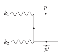
Figure 7: Fermion pair production from two photons.

Appendix B Fermion-antifermion pair annihilation into $3\gamma$

The decay amplitude $f\bar{f}\to 3\gamma$ to lowest order in $\alpha$ is given by the graph in Fig. 8 summed over the $3!$ permutations of the photons. The amplitude of the graph shown is

$$i{\cal M}=-ie^{3}Q_{f}^{3}\,\bar{v}(-\mathbf{p})\,{\hbox to0.0pt{$\epsilon_{3}$\hss}/}\,\,\frac{1}{-{\hbox to0.0pt{$p$\hss}/}^{\prime}+{\hbox to0.0pt{$k$\hss}/}_{3}-m}\,{\hbox to0.0pt{$\epsilon_{2}$\hss}/}\,\,\frac{1}{{\hbox to0.0pt{$p$\hss}/}-{\hbox to0.0pt{$k$\hss}/}_{1}-m}\,{\hbox to0.0pt{$\epsilon_{1}$\hss}/}\,\,u(\mathbf{p})\,.$$ (95)

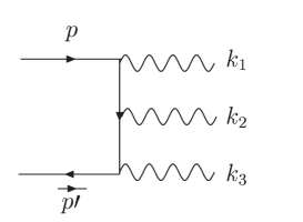
Figure 8: Three photon annihilation graph. The $3!$ permutations of the photons have to be considered.

We want to compute the leading term in the expansion of the three-momentum of the fermions in the c.m. frame $\mathbf{p}$. We can then work at threshold and the spinors reduce to

$$u(\mathbf{p})=\left(\begin{array}[]{c}\psi_{\mathbf{p}}\\ 0\end{array}\right)\;\;\;,\;\;\;v(\mathbf{p})=\left(\begin{array}[]{c}0\\ (i\sigma_{2})\chi_{\mathbf{p}}^{*}\end{array}\right)\,.$$ (100)

The leading term of the amplitude corresponding to the photon ordering in Fig. 8 then reads

$$i{\cal M}_{0}=-i\frac{e^{3}Q_{f}^{3}}{4m^{2}}\,\chi_{-\mathbf{p}}^{T}\,(-i\sigma_{2})\Big{[}(\bm{\sigma}\bm{\epsilon}_{3})(\bm{\sigma}\hat{\bm{k}}_{3})(\bm{\sigma}\bm{\epsilon}_{2})(\bm{\sigma}\hat{\bm{k}}_{1})(\bm{\sigma}\bm{\epsilon}_{1})+(\bm{\sigma}\bm{\epsilon}_{3})(\bm{\sigma}\bm{\epsilon}_{2})(\bm{\sigma}\bm{\epsilon}_{1})\Big{]}\psi_{\mathbf{p}}\,,$$

where $\hat{\bm{k}}_{i}=\bm{k}_{i}/\omega_{i}$ are the normalized three-momenta of the photons. If we add the graphs with different ordering of the photons and write the products of Pauli matrices in terms of the antisymmetric sigma tensors we obtain for the $f\bar{f}\to 3\gamma$ amplitude:

$$i{\cal M}_{0}=i\frac{e^{3}Q_{f}^{3}}{m^{2}}\,\chi_{-\mathbf{p}}^{T}\,(-i\sigma_{2})\!\!\! \bigg{(} \!\!\frac{m}{\omega_{3}}\epsilon_{1}^{i_{1}}\hat{k}_{1}^{i_{2}}\epsilon_{2}^{i_{3}}\hat{k}_{2}^{i_{4}}\epsilon_{3}^{i_{5}}\,\sigma^{i_{1}\ldots i_{5}}$$ (102)

$$\!\!\!\!\!\!\!\!\!\!\!\!\!\!\!\!\!-\frac{1}{2}\Big{[}\,f(1,2,3)\,{\epsilon}_{1}^{j}+g(1,2,3)\,\hat{k}_{1}^{j}+\{1\leftrightarrow 2\}+\{1\leftrightarrow 3\}\Big{]}\sigma^{j}\bigg{)}\psi_{\mathbf{p}}\,,$$

where

$$f(1,2,3) = \Big{(}1+(\hat{\bm{k}}_{2}\hat{\bm{k}}_{3})-(\hat{\bm{k}}_{1}\hat{\bm{k}}_{3})-(\hat{\bm{k}}_{1}\hat{\bm{k}}_{2})\Big{)}\,(\bm{\epsilon}_{2}\bm{\epsilon}_{3})$$

$$\;\;+(\hat{\bm{k}}_{1}\bm{\epsilon}_{3})\,(\hat{\bm{k}}_{3}\bm{\epsilon}_{2})+(\hat{\bm{k}}_{1}\bm{\epsilon}_{2})\,(\hat{\bm{k}}_{2}\bm{\epsilon}_{3})-(\hat{\bm{k}}_{3}\bm{\epsilon}_{2})\,(\hat{\bm{k}}_{2}\bm{\epsilon}_{3})$$

$$g(1,2,3) = \Big{(}(\hat{\bm{k}}_{3}\bm{\epsilon}_{1})+(\hat{\bm{k}}_{2}\bm{\epsilon}_{1})\Big{)}\,(\bm{\epsilon}_{2}\bm{\epsilon}_{3})-(\bm{\epsilon}_{1}\bm{\epsilon}_{3})\,(\hat{\bm{k}}_{3}\bm{\epsilon}_{2})-(\bm{\epsilon}_{1}\bm{\epsilon}_{2})\,(\hat{\bm{k}}_{2}\bm{\epsilon}_{3})\,.$$ (103)

Note that the $\sigma^{i_{1}i_{2}i_{3}}$ terms cancel when summing over permutations of the photons.

Appendix C Tensor decompositions

C.1 $T^{i_{1}\dots i_{L}}\,\sigma^{i_{L+1}}$

The space of traceless tensors of rank $L+1$ formed from the product of the $T^{i_{1}\dots i_{L}}(\mathbf{p})$ and $\sigma^{i_{L+1}}$, $\langle\,T^{i_{1}\dots i_{L}}\sigma^{i_{L+1}}\rangle$, is obtained by removing the traces of $T^{i_{1}\dots i_{L}}\sigma^{i_{L+1}}$:

$$\langle\,T^{i_{1}\dots i_{L}}\sigma^{i_{L+1}}\rangle = T^{i_{1}\dots i_{L}}\sigma^{i_{L+1}}-\frac{1}{L+n-3}\sum_{k=1}^{L}\delta^{i_{k}i_{L+1}}\Gamma^{S=1}_{L-1}(\mathbf{p},\mathbf{\mbox{\boldmath$\sigma$}})^{i_{1}\dots\,\,\!\widehat{\!\textit{\i}}_{k}\dots i_{L}}$$ (104)

$$+\frac{2}{(L+n-3)(2L+n-2)}\sum_{k=1\atop k<m}^{L+1}\delta^{i_{k}i_{m}}\Gamma^{S=1}_{L-1}(\mathbf{p},\mathbf{\mbox{\boldmath$\sigma$}})^{i_{1}\dots\,\,\!\widehat{\!\textit{\i}}_{k}\dots\,\,\!\widehat{\!\textit{\i}}_{m}\dots i_{L+1}}\,,$$

with the tensors $\Gamma^{S=1}_{L-1}$ defined in Eq. (32). This space has dimension $n_{L}\cdot n-n_{L-1}$ and is not irreducible. From the resolution of the identity in terms of Young operators of the symmetric group $S_{L+1}$ grouptheory (see Fig. 9),

Figure 9: Resolution of the identity in terms of Young operators of the symmetric group $S_{L+1}$ accounting also for the proper Hook factors Georgi . We have only shown the Young patterns which give a nonzero result when acting on the indices of $T^{i_{1}\dots i_{L}}\sigma^{i_{L+1}}$. We shall use $[L+1]$ to denote the first pattern, and $[L,1]$ for the pattern with $L$ boxes in the first row and one in the second. There are $L$ standard tableaux for the pattern $[L,1]$. We adopt the convention that symmetrization horizontally top-to-down is followed by antisymmetrization vertically left-to-right.

which act on the indices of the tensors, we can decompose $\langle\,T^{i_{1}\dots i_{L}}\sigma^{i_{L+1}}\rangle$ into traceless tensors of a given symmetry type:

$$\langle\,T^{i_{1}\dots i_{L}}\sigma^{i_{L+1}}\rangle = \frac{1}{L+1}\,\Gamma^{S=1}_{L+1}(\mathbf{p},\mathbf{\mbox{\boldmath$\sigma$}})^{i_{1}\dots i_{L+1}}$$ (105)

$$+\,\frac{L}{L+1}\,\widetilde{\Gamma}^{S=1}_{L}(\mathbf{p},\mathbf{\mbox{\boldmath$\sigma$}})^{i_{2}\dots i_{L}}_{[i_{1}i_{L+1}]}-\frac{1}{L+1}\,\sum_{k=2}^{L}\,\widetilde{\Gamma}^{S=1}_{L}(\mathbf{p},\mathbf{\mbox{\boldmath$\sigma$}})^{i_{2}\dots\,\,\!\widehat{\!\textit{\i}}_{k}\ldots i_{L+1}}_{[i_{1}i_{k}]}\,.$$

The first term in Eq. (105) results from the application of the first tableau in Fig. 9 (the pattern $[L+1]$) to the tensor $\langle\,T^{i_{1}\dots i_{L}}\sigma^{i_{L+1}}\rangle$, which yields a totally symmetric tensor. This is the tensor used to define the $J=L+1$ triplet current in Sec. III, and its explicit form is given in Eq. (LABEL:tripletcurrent1). The $L$ terms in the second an third lines of Eq. (105) correspond to the $L$ Young tableaux with the pattern $[L,1]$ shown in Fig. 9. These tensors read

$$\widetilde{\Gamma}^{S=1}_{L}(\mathbf{p},\mathbf{\mbox{\boldmath$\sigma$}})_{[i_{1}i_{m}]}^{i_{2}\ldots\,\,\!\widehat{\!\textit{\i}}_{m}\ldots i_{L+1}}\,\equiv\,$$ (106)

$$\equiv\,T^{\,i_{1}\dots\,\,\!\widehat{\!\textit{\i}}_{m}\dots i_{L+1}}\,\sigma^{i_{m}}-\frac{1}{L+n-3}\sum_{k=2\atop k\neq m}^{L+1}\,\delta^{i_{k}i_{m}}\,T^{\,i_{1}\dots\,\,\!\widehat{\!\textit{\i}}_{k}\dots\,\,\!\widehat{\!\textit{\i}}_{m}\dots i_{L+1}\ell}\,\sigma^{\ell}-\{i_{1}\leftrightarrow i_{m}\}\,,$$

and have dimension ($L\geq 1$)

$$d_{[L,1]}\,=\,n_{L}\cdot n-n_{L-1}-n_{L+1}\,=\,\frac{\Gamma(n+L-1)}{\Gamma(n-2)\Gamma(L+2)}\frac{L(2L+n-2)}{L+n-3}\,,$$ (107)

which for $n=3$ reduces to $2L+1$. Indeed, the tensors corresponding to the pattern $[L]$ in Eq. (33) and those corresponding to the pattern $[L,1]$ in Eq. (106), although transforming according to different irreducible representations of SO(n), become equivalent in $n=3$, and thus represent both appropriate candidates for defining the triplet current with quantum numbers $J=L$ in dimensional regularization. This justifies the quantum numbers used to label the currents in Eq. (106).

As the tensor $\langle\,T^{i_{1}\dots i_{L}}\sigma^{i_{L+1}}\rangle$ is already symmetric on the $i_{1}\dots i_{L}$ indices, the subspaces which result from the action of the different $[L,1]$ tableaux are all equivalent. Therefore the space $\langle\,T^{i_{1}\dots i_{L}}\sigma^{i_{L+1}}\rangle$ decomposes into a subspace of totally symmetric tensors, of dimension $n_{L+1}$, and a subspace of tensors which transform equivalently to the irreducible representation of SO(n) defined by the symmetry pattern $[L,1]$, of dimension $d_{[L,1]}$. Thus the second and third lines in Eq. (105) should not be understood as a tensor decomposition into orthogonal subspaces, but as a convenient way to write the components of a tensor of this subspace in terms of tensors of the symmetry type given by the Young tableaux.

The results in Eqs. (104) and (105) show how the reducible tensor $A^{i_{1}\cdots i_{L+1}}=\psi_{\mathbf{p}}^{\dagger}\,T^{i_{1}\dots i_{L}}(\mathbf{p})\sigma^{i_{L+1}}(i\sigma_{2})\chi_{-\mathbf{p}}^{*}$ can be fully written in terms of the currents defined from the tensors $\Gamma^{S=1}_{L+1}\,,\widetilde{\Gamma}^{S=1}_{L}$ and $\Gamma^{S=1}_{L-1}$. The latter current already emerges in Eq. (104) when eliminating the traces from $T^{i_{1}\dots i_{L}}\sigma^{i_{L+1}}$.

C.2 $T^{i_{1}\dots i_{L}}\,\sigma^{i_{L+1}i_{L+2}}$

The reduction of the tensor $T^{i_{1}\dots i_{L}}(\mathbf{p})\sigma^{i_{L+1}i_{L+2}}$ can be carried out in a similar way. The traceless tensor $\langle\,T^{i_{1}\dots i_{L}}(\mathbf{p})\sigma^{i_{L+1}i_{L+2}}\,\rangle$, of dimension $n_{L}\frac{n(n-1)}{2}-n_{L-1}\cdot n+n_{L-2}$, reads

$$\langle\,T^{i_{1}\dots i_{L}}\sigma^{i_{L+1}i_{L+2}}\rangle = T^{i_{1}\dots i_{L}}\sigma^{i_{L+1}i_{L+2}}-c_{1}\sum_{k=1\atop k<m}^{L}\,\delta^{i_{k}i_{m}}\,\widetilde{\Gamma}^{S=1}_{L-1}(\mathbf{p},\mathbf{\mbox{\boldmath$\sigma$}})^{i_{1}\dots\,\,\!\widehat{\!\textit{\i}}_{k}\ldots\,\,\!\widehat{\!\textit{\i}}_{m}\ldots i_{L}}_{[i_{L+1}i_{L+2}]}$$

$$-c_{0}(1-\delta_{L,1})\,\bigg{[}\sum_{k=1}^{L}\,\delta^{i_{k}i_{L+1}}\,\Gamma^{S=1}_{L}(\mathbf{p},\mathbf{\mbox{\boldmath$\sigma$}})^{i_{1}\dots\,\,\!\widehat{\!\textit{\i}}_{k}\ldots i_{L}i_{L+2}}-\{i_{L+1}\leftrightarrow i_{L+2}\}\bigg{]}$$

$$-(c_{0}+c_{2})\,\bigg{[}\sum_{k,m=1\atop k\neq m}^{L}\,\delta^{i_{k}i_{L+1}}\,\widetilde{\Gamma}^{S=1}_{L-1}(\mathbf{p},\mathbf{\mbox{\boldmath$\sigma$}})^{i_{1}\dots\,\,\!\widehat{\!\textit{\i}}_{k}\ldots\,\,\!\widehat{\!\textit{\i}}_{m}\ldots i_{L}}_{[i_{m}i_{L+2}]}-\{i_{L+1}\leftrightarrow i_{L+2}\}\bigg{]}\,,$$

with

$$c_{0}=\frac{1}{(L-1)(L+n-2)}\;\;,\;\;c_{1}=-\frac{2}{(2L+n-2)\,(L+n-4)}\,,$$

$$c_{2}=\frac{2}{(2L+n-2)\,(L+n-4)\,(L+n-2)}\,,$$

and

$$\widetilde{\Gamma}^{S=1}_{L-1}(\mathbf{p},\mathbf{\mbox{\boldmath$\sigma$}})_{[i_{1}i_{m}]}^{i_{2}\ldots\,\,\!\widehat{\!\textit{\i}}_{m}\ldots i_{L}}\,\equiv\,T^{\,i_{1}\dots\,\,\!\widehat{\!\textit{\i}}_{m}\dots i_{L}\ell}\,\sigma^{\ell\,i_{m}}-T^{\,i_{2}\dots i_{L}\ell}\,\sigma^{\ell\,i_{1}}\,.$$ (109)

The latter is a tensor which transforms according to the representation defined by the pattern $[L,1]$, so for $n=3$ it is equivalent to the totally symmetric tensor $\Gamma^{S=1}_{L-1}(\mathbf{p},\mathbf{\mbox{\boldmath$\sigma$}})^{i_{1}\dots i_{L-1}}$ defined in Eq. (32) with $L-1$ indices.

The space $\langle\,T^{i_{1}\dots i_{L}}(\mathbf{p})\sigma^{i_{L+1}i_{L+2}}\,\rangle$ can be written in terms of tensors with the symmetry type given by the standard Young tableaux which appear in the resolution of the identity of the symmetric group $S_{L+2}$ shown in Fig. 10:

Figure 10: Resolution of the identity in terms of Young operators of the symmetric group $S_{L+2}$. We have only shown the Young patterns which give a nonzero result when acting on the indices of $T^{i_{1}\dots i_{L}}\sigma^{i_{L+1}i_{L+2}}$. There are in total $2(L-1)$ tableaux in the second line.

$$\langle\,T^{i_{1}\dots i_{L}}\sigma^{i_{L+1}i_{L+2}}\rangle = \frac{1}{L+2}\,\widetilde{\Gamma}^{S=1}_{L+1}(\mathbf{p},\mathbf{\mbox{\boldmath$\sigma$}})^{i_{2}\dots\,\,\!\widehat{\!\textit{\i}}_{L+1}i_{L+2}}_{[i_{1}i_{L+1}]}-\frac{1}{L+2}\,\widetilde{\Gamma}^{S=1}_{L+1}(\mathbf{p},\mathbf{\mbox{\boldmath$\sigma$}})^{i_{2}\dots i_{L+1}}_{[i_{1}i_{L+2}]}+\dots\,$$ (110)

The first and second terms in Eq. (110) correspond to the action of the two Young tableaux with the pattern $[L+1,1]$ in Fig. 10. The explicit form of these tensors read

$$\widetilde{\Gamma}^{S=1}_{L+1}(\mathbf{p},\mathbf{\mbox{\boldmath$\sigma$}})^{i_{2}\dots i_{L+1}}_{[i_{1}i_{L+2}]} = T^{\,i_{2}\dots i_{L+1}}\,\sigma^{i_{1}i_{L+2}}+\sum_{k=2}^{L+1}\,T^{\,i_{1}\dots\,\,\!\widehat{\!\textit{\i}}_{k}\dots i_{L+1}}\,\sigma^{i_{k}i_{L+2}}$$

$$-\,f_{1}\,\sum_{k<j\atop k=2}^{L+1}\,\delta^{i_{k}i_{j}}\,T^{\,i_{1}\dots\,\,\!\widehat{\!\textit{\i}}_{k}\dots\,\,\!\widehat{\!\textit{\i}}_{j}\dots i_{L+1}\ell}\,\sigma^{\ell\,i_{L+2}}$$

$$-\,f_{2}\,\sum_{k\neq j\atop k,j=2}^{L+1}\,\delta^{i_{1}i_{k}}\,T^{\,i_{2}\dots\,\,\!\widehat{\!\textit{\i}}_{k}\dots\,\,\!\widehat{\!\textit{\i}}_{j}\dots i_{L+2}\ell}\,\sigma^{\ell\,i_{j}}$$

$$-\,(f_{1}+f_{2})\,\sum_{k=2}^{L+1}\,\delta^{i_{1}i_{k}}\,T^{\,i_{2}\dots\,\,\!\widehat{\!\textit{\i}}_{k}\dots i_{L+1}\ell}\,\sigma^{\ell\,i_{L+2}}-\{i_{1}\leftrightarrow i_{L+2}\}\,,$$

$$f_{1}= \!\!\!\!\!\!\!\frac{2}{2L+n-2}\quad,\quad f_{2}=\frac{2L+n}{(L+n-2)(2L+n-2)}\;.$$ (111)

The dots in Eq. (110) stand for the tensors associated to the rest of the Young tableaux in Fig. 10. We do not give their explicit form because they are evanescent and vanish for $n=3$, as the traceless tensors corresponding to Young patterns in which the sum of the lengths of the first two columns exceeds $n$ are identically zero grouptheory  . Eqs. (LABEL:Tss_traceless) and (110) give the decomposition of the tensor $B^{i_{1}\cdots i_{L+2}}=\psi_{\mathbf{p}}^{\dagger}\,T^{i_{1}\dots i_{L}}(\mathbf{p})\sigma^{i_{L+1}i_{L+2}}(i\sigma_{2})\chi_{-\mathbf{p}}^{*}$ into the currents built from the irreducible tensors $\widetilde{\Gamma}^{S=1}_{L\pm 1}$ and $\Gamma^{S=1}_{L}$, that have fixed quantum numbers in $n=3$.

The three new spin triplet currents $\psi_{\mathbf{p}}^{\dagger}\,\widetilde{\Gamma}^{S=1}_{J}(i\sigma_{2})\chi_{-\mathbf{p}}^{*}$ introduced above, Eqs. (106,109,111), have $2J+1$ independent components in $n=3$ dimensions and differ from the basis of currents defined in Sec. III in the symmetry patterns and the number of indices. The following relations among the tensors $\Gamma^{S=1}_{J}$ and $\widetilde{\Gamma}^{S=1}_{J}$ with the same quantum numbers hold for $n=3$:

$$\widetilde{\Gamma}^{S=1}_{L+1}(\mathbf{p},\mathbf{\mbox{\boldmath$\sigma$}})^{i_{2}\dots i_{L+1}}_{[j_{1}j_{L+2}]} = i\,\frac{L+2}{L+1}\,\epsilon^{\,i_{1}j_{1}j_{L+2}}\,\Gamma^{S=1}_{L+1}(\mathbf{p},\mathbf{\mbox{\boldmath$\sigma$}})^{i_{1}\dots i_{L+1}}\,,$$

$$\widetilde{\Gamma}^{S=1}_{L}(\mathbf{p},\mathbf{\mbox{\boldmath$\sigma$}})^{i_{2}\dots i_{L}}_{[j_{1}j_{L+1}]} = \frac{i}{L}\,\epsilon^{\,i_{1}j_{1}j_{L+1}}\,\Gamma^{S=1}_{L}(\mathbf{p},\mathbf{\mbox{\boldmath$\sigma$}})^{i_{1}\dots i_{L}}\,,$$

$$\widetilde{\Gamma}^{S=1}_{L-1}(\mathbf{p},\mathbf{\mbox{\boldmath$\sigma$}})^{i_{2}\dots i_{L-1}}_{[j_{1}j_{L}]} = -i\,\epsilon^{\,i_{1}j_{1}j_{L}}\,\Gamma^{S=1}_{L-1}(\mathbf{p},\mathbf{\mbox{\boldmath$\sigma$}})^{i_{1}\dots i_{L-1}}\,.$$ (112)

For completeness, we also give the total contraction of the $\widetilde{\Gamma}^{S=1}_{J}$ tensors:

$$\mbox{Tr}\Big{[}\widetilde{\Gamma}^{S=1\,\dagger}_{L+1}(\mathbf{p},\mathbf{\mbox{\boldmath$\sigma$}})^{i_{2}\dots\dots i_{L+1}}_{[i_{1}i_{L+2}]}\,\widetilde{\Gamma}^{S=1}_{L+1}(\mathbf{q},\mathbf{\mbox{\boldmath$\sigma$}})^{i_{2}\dots\dots i_{L+1}}_{[i_{1}i_{L+2}]}\Big{]} = \frac{2(n-2)(L+2)(2L+n)(L+n-1)}{2L+n-2}$$

$$\qquad\times\,T_{L,n}(\mathbf{p},\mathbf{q})\mbox{Tr}\,[\mathbf{1}]\,,$$

$$\mbox{Tr}\Big{[}\widetilde{\Gamma}^{S=1\,\dagger}_{L}(\mathbf{p},\mathbf{\mbox{\boldmath$\sigma$}})^{i_{2}\dots i_{L}}_{[i_{1}i_{L+1}]}\,\widetilde{\Gamma}^{S=1}_{L}(\mathbf{q},\mathbf{\mbox{\boldmath$\sigma$}})^{i_{2}\dots i_{L}}_{[i_{1}i_{L+1}]}\Big{]} = 2(n-2)\,\frac{L+n-2}{L+n-3}\,T_{L,n}(\mathbf{p},\mathbf{q})\mbox{Tr}\,[\mathbf{1}]\,,$$

$$\mbox{Tr}\Big{[}\widetilde{\Gamma}^{S=1\,\dagger}_{L-1}(\mathbf{p},\mathbf{\mbox{\boldmath$\sigma$}})_{[i_{1}i_{L}]}^{i_{2}\ldots i_{L-1}}\,\widetilde{\Gamma}^{S=1}_{L-1}(\mathbf{q},\mathbf{\mbox{\boldmath$\sigma$}})_{[i_{1}i_{L}]}^{i_{2}\ldots i_{L-1}}\Big{]} = 2(n-2)\,T_{L,n}(\mathbf{p},\mathbf{q})\mbox{Tr}\,[\mathbf{1}]\,.$$ (113)

To conclude this section we mention that the guidelines of constructing nonrelativistic currents that are irreducible under SO(n), as shown above, can be generalized in a straightforward way to currents containing $\sigma^{i_{1}\dots i_{m}}$ with $m>2$. For larger $m$, the number of evenescent currents will increase. A very helpful rule to identify these currents is the rule that traceless tensors corresponding to Young patterns in which the sum of the lengths of the first two columns exceeds $n$ are identically zero grouptheory .

Appendix D Useful integrals

We list in this appendix the results for the relevant integrals needed for the determination of the UV-divergences of the three-loop correlators in Secs. IV and V. Note that Greek letters $\alpha,\beta,\gamma,\ldots$ refer to real numbers while $k,r$ denote positive integers.

We define the following integrals:

$$\mbox{I}^{(k)}[\alpha,\beta,\gamma] \equiv \int\frac{d^{n}\mathbf{p}}{(2\pi)^{n}}\frac{d^{n}\mathbf{q}}{(2\pi)^{n}}\,\frac{(\mathbf{p}.\mathbf{q})^{k}}{[\mathbf{p}^{2}+\delta]^{\alpha}\,[(\mathbf{p}-\mathbf{q})^{2}]^{\beta}\,[\mathbf{q}^{2}+\delta]^{\gamma}}\,,$$ (114)

$$\mbox{I}^{(k)}[\alpha,\beta,\gamma,\rho,\sigma] \equiv \int\frac{d^{n}\mathbf{p}}{(2\pi)^{n}}\frac{d^{n}\bm{\ell}}{(2\pi)^{n}}\frac{d^{n}\mathbf{q}}{(2\pi)^{n}}\,\frac{(\mathbf{p}.\mathbf{q})^{k}}{[\mathbf{p}^{2}+\delta]^{\alpha}\,[(\mathbf{p}-\bm{\ell})^{2}]^{\beta}\,[\bm{\ell}^{2}+\delta]^{\gamma}\,[(\bm{\ell}-\mathbf{q})^{2}]^{\rho}\,[\mathbf{q}^{2}+\delta]^{\sigma}}\,,$$

$$\mbox{J}[\alpha,\beta,\gamma,\rho,\sigma] \equiv \int\frac{d^{n}\mathbf{p}}{(2\pi)^{n}}\frac{d^{n}\bm{\ell}}{(2\pi)^{n}}\frac{d^{n}\mathbf{q}}{(2\pi)^{n}}\,\frac{1}{[\mathbf{p}^{2}+\delta]^{\alpha}\,[(\mathbf{p}-\bm{\ell})^{2}]^{\beta}\,[\bm{\ell}^{2}]^{\gamma}\,[(\bm{\ell}-\mathbf{q})^{2}]^{\rho}\,[\mathbf{q}^{2}+\delta]^{\sigma}}\,.\qquad$$ (116)

For the spin-independent potentials the required UV-divergent terms are:

$$\mbox{I}^{(k)}[1,\frac{1}{2},1]_{\rm div} = (-1)^{k+1}\,{}_{2}F_{1}\Big{(}\frac{1}{2},-k,\frac{3}{2},2\Big{)}\,\frac{\delta^{k+\frac{1}{2}}}{8\pi^{3}\,\epsilon}+{\cal O}(\epsilon^{0})\,,$$ (117)

$$\mbox{I}^{(k)}[1,2-\frac{n}{2},1]_{\rm div} = (-1)^{k+1}\,{}_{2}F_{1}\Big{(}\frac{1}{2},-k,\frac{3}{2},2\Big{)}\,\frac{\delta^{k+\frac{1}{2}}}{16\pi^{3}\,\epsilon}+{\cal O}(\epsilon^{0})\,,$$ (118)

$$\mbox{I}^{(k)}[1,1,0,1,1]_{\rm div}=(-1)^{k+1}\,{}_{2}F_{1}\Big{(}\frac{1}{2},-k,\frac{3}{2},2\Big{)}\,\frac{\delta^{k+\frac{1}{2}}}{128\pi^{3}\,\epsilon}+{\cal O}(\epsilon^{0})\,,$$ (119)

$$\mbox{I}^{(2k)}[1,0,1,1,1]_{\rm div}=-\frac{1}{1+2k}\,\frac{\delta^{2k+\frac{1}{2}}}{256\pi^{3}\,\epsilon}+{\cal O}(\epsilon^{0})\,.$$

The spin-dependent contributions require:

$$\mbox{J}[1,1,-k,1,1]_{\rm div} = (-1)^{k+1}\frac{1}{1+2k}\,\frac{\delta^{k+\frac{1}{2}}}{128\pi^{3}\epsilon}+{\cal O}(\epsilon^{0})\,,$$ (120)

$$\mbox{J}[1,-k,r,1,1]_{\rm div} = (-1)^{k-r}\frac{\Gamma(2k+2)}{\Gamma(2k-2r+4)\Gamma(2r)}\,\frac{\delta^{k-r+\frac{3}{2}}}{256\pi^{3}\epsilon}+{\cal O}(\epsilon^{0})\,,$$ (121)

$$\mbox{I}^{(0)}[1,1,-k,1,1]_{\rm div} = -\frac{\sqrt{\pi}\,\Gamma(k+1)}{\Gamma(k+\frac{3}{2})}\,\frac{\delta^{k+\frac{1}{2}}}{256\pi^{3}\epsilon}+{\cal O}(\epsilon^{0})\,,$$ (122)

$$\mbox{I}^{(0)}[1,-k,1,1,1]_{\rm div} = (-1)^{k+1}\frac{2^{2k-8}}{1+k}\,\frac{\delta^{k+\frac{1}{2}}}{\pi^{3}\epsilon}+{\cal O}(\epsilon^{0})\,.$$ (123)

References

• (1) N. Brambilla, A. Pineda, J. Soto and A. Vairo, Rev. Mod. Phys.  77 (2005) 1423 [arXiv:hep-ph/0410047]; N. Brambilla et al., arXiv:hep-ph/0412158; A. H. Hoang, arXiv:hep-ph/0204299; I. Z. Rothstein, arXiv:hep-ph/9911276; M. Beneke, arXiv:hep-ph/9703429.
• (2) W.E. Caswell and G.P. Lepage, Phys. Lett. 167B, 437 (1986).
• (3) G.T. Bodwin, E. Braaten and G.P. Lepage, Phys. Rev. D51, 1125 (1995), ibid. D55, 5853 (1997).
• (4) P. Labelle, Phys. Rev. D58, 093013 (1998) [arXiv:hep-ph/9608491].
• (5) M. Luke and A.V. Manohar, Phys. Rev. D55, 4129 (1997) [arXiv:hep-ph/9610534].
• (6) B. Grinstein and I.Z. Rothstein, Phys. Rev. D57, 78 (1998) [arXiv:hep-ph/9703298].
• (7) M. Luke and M.J. Savage, Phys. Rev. D57, 413 (1998) [arXiv:hep-ph/9707313].
• (8) A. Pineda and J. Soto, Nucl. Phys. Proc. Suppl. 64, 428 (1998) [arXiv:hep-ph/9707481].
• (9) A. Pineda and J. Soto, Phys. Rev. D58, 114011 (1998) [arXiv:hep-ph/9802365].
• (10) A. Pineda and J. Soto, Phys. Rev. D 59, 016005 (1999) [arXiv:hep-ph/9805424].
• (11) M. Luke, A. Manohar and I. Rothstein, Phys. Rev.  D61, 074025 (2000) [arXiv:hep-ph/9910209].
• (12) A.V. Manohar and I.W. Stewart, Phys. Rev. Lett.  85, 2248 (2000) [arXiv:hep-ph/0004018].
• (13) A.V. Manohar, J. Soto, and I.W. Stewart, Phys. Lett. B486, 400 (2000) [arXiv:hep-ph/0006096].
• (14) A. H. Hoang and I. W. Stewart, Phys. Rev. D 67, 114020 (2003) [arXiv:hep-ph/0209340].
• (15) A. H. Hoang, Phys. Rev. D 69, 034009 (2004) [arXiv:hep-ph/0307376].
• (16) A.V. Manohar and I.W. Stewart, Phys. Rev. D 62, 014033 (2000) [arXiv:hep-ph/9912226].
• (17) A.V. Manohar and I.W. Stewart, Phys. Rev.  D62, 074015 (2000) [arXiv:hep-ph/0003032].
• (18) A.V. Manohar and I.W. Stewart, Phys. Rev. D63, 054004 (2001). [arXiv:hep-ph/0003107].
• (19) A. H. Hoang and P. Ruiz-Femenia, Phys. Rev. D 73, 014015 (2006) [arXiv:hep-ph/0511102].
• (20) A. Pineda and J. Soto, Phys. Lett. B495, 323 (2000) [arXiv:hep-ph/0007197].
• (21) A. Pineda, Phys. Rev. D 65, 074007 (2002) [arXiv:hep-ph/0109117].
• (22) A. Pineda, Phys. Rev. D 66, 054022 (2002) [arXiv:hep-ph/0110216].
• (23) A. Pineda, arXiv:hep-ph/0204213.
• (24) A. A. Penin, A. Pineda, V. A. Smirnov and M. Steinhauser, Phys. Lett. B 593, 124 (2004) [arXiv:hep-ph/0403080].
• (25) A. A. Penin, A. Pineda, V. A. Smirnov and M. Steinhauser, Nucl. Phys. B 699, 183 (2004) [arXiv:hep-ph/0406175].
• (26) M. Stahlhofen, Diploma thesis, TU Munich, April 2005 .
• (27) J. A. Aguilar-Saavedra et al. [ECFA/DESY LC Physics Working Group Collaboration], arXiv:hep-ph/0106315; T. Abe et al. [American Linear Collider Working Group Collaboration], in Proc. of the APS/DPF/DPB Summer Study on the Future of Particle Physics (Snowmass 2001) ed. N. Graf, arXiv:hep-ex/0106057.
• (28) A. H. Hoang, A. V. Manohar, I. W. Stewart and T. Teubner, Phys. Rev. Lett.  86, 1951 (2001) [arXiv:hep-ph/0011254].
• (29) A. H. Hoang, A. V. Manohar, I. W. Stewart and T. Teubner, Phys. Rev. D 65, 014014 (2002) [arXiv:hep-ph/0107144].
• (30) A. H. Hoang and T. Teubner, Phys. Rev. D 58, 114023 (1998) [arXiv:hep-ph/9801397];
A. H. Hoang and T. Teubner, Phys. Rev. D 60, 114027 (1999) [arXiv:hep-ph/9904468].
• (31) A. H. Hoang et al., in Eur. Phys. J. direct C3, 1 (2000) [arXiv:hep-ph/0001286].
• (32) C. Farrell and A. H. Hoang, Phys. Rev. D 72, 014007 (2005) [arXiv:hep-ph/0504220].
• (33) C. Farrell and A. H. Hoang, Phys. Rev. D 74, 014008 (2006) [arXiv:hep-ph/0604166].
• (34) M. J. Dugan and B. Grinstein, Phys. Lett. B 256, 239 (1991).
• (35) S. Herrlich and U. Nierste, Nucl. Phys. B 455, 39 (1995) [arXiv:hep-ph/9412375].
• (36) K. G. Chetyrkin, M. Misiak and M. Munz, Nucl. Phys. B 520, 279 (1998) [arXiv:hep-ph/9711280].
• (37) A.H. Hoang, A.V. Manohar and I.W. Stewart, Phys. Rev. D 64, 014033 (2001) [arXiv:hep-ph/0102257].
• (38) K. Melnikov and A. Yelkhovsky, Phys. Rev. D 59, 114009 (1999) [arXiv:hep-ph/9805270].
• (39) J. M. Normand and J. Raynal, J. Phys. A 15, 1437 (1982).
• (40) See e.g. M. Hamermesh, “Group theory and its application to physical problems,”, Dover Publ., 1989.
• (41) I.S. Gradshteyn and I.M. Ryzhik, “Table of integrals, series and products”, 5th ed., Academic Press, 1994.
• (42) V. S. Fadin and V. A. Khoze, Sov. J. Nucl. Phys.  53, 692 (1991) [Yad. Fiz.  53, 1118 (1991)].
• (43) M. Beneke and V.A. Smirnov, Nucl. Phys. B522, 321 (1998) [arXiv:hep-ph/9711391].
• (44) A. Czarnecki and K. Melnikov, Phys. Rev. Lett.  80, 2531 (1998) [arXiv:hep-ph/9712222].
• (45) M. Beneke, A. Signer and V. A. Smirnov, Phys. Rev. Lett.  80, 2535 (1998) [arXiv:hep-ph/9712302].
• (46) A. Czarnecki and K. Melnikov, Phys. Rev. D 65, 051501 (2002) [arXiv:hep-ph/0108233].
• (47) B. A. Kniehl, A. Onishchenko, J. H. Piclum and M. Steinhauser, Phys. Lett. B 638, 209 (2006) [arXiv:hep-ph/0604072].
• (48) M. Beneke, A. Signer and V. A. Smirnov, Phys. Lett. B 454 (1999) 137 [arXiv:hep-ph/9903260].
• (49) S. Titard and F. J. Yndurain, Phys. Rev. D 49, 6007 (1994) [arXiv:hep-ph/9310236].
• (50) V. S. Fadin and V. A. Khoze, Sov. J. Nucl. Phys.  48, 309 (1988) [Yad. Fiz.  48, 487 (1988)].
• (51) M. Jezabek, J. H. Kuhn and T. Teubner, Z. Phys. C 56 (1992) 653.
• (52) A. Pineda and A. Signer, arXiv:hep-ph/0607239.
• (53) H. Georgi, “Lie algebras in particle physics”, 2nd ed., Westview Press, 1999.