Mesonic correlation functions at finite temperature and density in the Nambu – Jona - Lasinio model with a Polyakov loop

Abstract

We investigate the properties of scalar and pseudo-scalar mesons at finite temperature and quark chemical potential in the framework of the Nambu–Jona-Lasinio (NJL) model coupled to the Polyakov loop (PNJL model) with the aim of taking into account features of both chiral symmetry breaking and deconfinement.

The mesonic correlators are obtained by solving the Schwinger–Dyson equation in the RPA approximation with the Hartree (mean field) quark propagator at finite temperature and density.

In the phase of broken chiral symmetry a narrower width for the $\sigma$ meson is obtained with respect to the NJL case; on the other hand, the pion still behaves as a Goldstone boson.

When chiral symmetry is restored, the pion and $\sigma$ spectral functions tend to merge. The Mott temperature for the pion is also computed.

I Introduction

Recently, increasing attention has been devoted to study the modification of particles propagating in a hot or dense medium manna ; kita . The possible survival of bound states in the deconfined phase of QCD datta1 ; shury1 ; shury2 ; wong1 ; wong2 ; datta2 ; albe ; mocsy has opened interesting scenarios for the identification of the relevant degrees of freedom in the vicinity of the phase transition koch ; ej ; shury3 . At the same time, renewed interest has arisen for the study of the $\rho$ meson spectral function in a hot medium renk1 ; renk2 ; rapp1 ; rapp2 ; rho1 ; rho2 , since precise experimental data have now become available for this observable na60 .

In this paper, we focus on the description of light scalar and pseudo-scalar mesons at finite temperature and quark chemical potential. Besides lattice calculations taro ; taro2 ; petr ; wis , high temperature correlators between mesonic current operators can be studied, starting from the QCD lagrangian, within different theoretical schemes, like the dimensional reduction za ; lai or the Hard Thermal Loop approximation berry ; berry2 ; mus . Actually both the above approaches rely on a separation of momentum scales which, strictly speaking, holds only in the weak coupling regime $g\ll 1$. Hence they cannot tell us anything about what happens in the vicinity of the phase transition.

On the other hand a system close to a phase transition is characterized by large correlation lengths (infinite in the case of a second order phase transition). Its behaviour is mainly driven by the symmetries of the lagrangian, rather than by the details of the microscopic interactions. In this critical regime of temperatures and densities our investigation of meson properties is then performed in the framework of an effective model of QCD, namely a modified Nambu Jona-Lasinio model including Polyakov loop dynamics (referred to as PNJL model)  Meisinger:1995ih ; Meisinger:2001cq ; Fukushima:2003fw ; Mocsy:2003qw ; Megias:2004hj ; Ratti:2005jh ; Ratti:2006gh ; mus2 .

Models of the Nambu and Jona-Lasinio (NJL) type NJL61 have a long history and have been extensively used to describe the dynamics and thermodynamics of the lightest hadrons Hatsuda:1985eb ; Bernard:1987im ; Bernard:1987ir ; Jaminon:1989wp ; VW91 ; Klevansky:1992qe ; Lutz:1992dv ; HK94 ; Bernard:1990ye ; Ri97 . Such schematic models offer a simple and practical illustration of the basic mechanisms that drive the spontaneous breaking of chiral symmetry, a key feature of QCD in its low-temperature, low-density phase.

In first approximation the behavior of a system ruled by QCD is governed by the symmetry properties of the Lagrangian, namely the (approximate) global symmetry $SU_{L}(N_{f})\times SU_{R}(N_{f})$, which is spontaneously broken to $SU_{V}(N_{f})$ and the (exact) $SU_{c}(N_{c})$ local color symmetry. Indeed in the NJL model the mass of a constituent quark is directly related to the chiral condensate, which is the order parameter of the chiral phase transition and, hence, is non-vanishing at zero temperature and density. Here the system lives in the phase of spontaneously broken chiral symmetry: the strong interaction, by polarizing the vacuum and turning it into a condensate of quark-antiquark pairs, transforms an initially point-like quark with its small bare mass $m_{0}$ into a massive quasiparticle with a finite size. Despite their widespread use, NJL models suffer a major shortcoming: the reduction to global (rather than local) colour symmetry prevents quark confinement.

On the other hand, in a non-abelian pure gauge theory, the Polyakov loop serves as an order parameter for the transition from the low temperature, $\mathbb{Z}_{N_{c}}$ symmetric, confined phase (the active degrees of freedom being color-singlet states, the glueballs), to the high temperature, deconfined phase (the active degrees of freedom being colored gluons), characterized by the spontaneous breaking of the $\mathbb{Z}_{N_{c}}$ (center of $SU_{c}(N_{c})$) symmetry.

With the introduction of dynamical quarks, this symmetry breaking pattern is no longer exact: nevertheless it is still possible to distinguish a hadronic (confined) phase from a QGP (deconfined) one.

In the PNJL model quarks are coupled simultaneously to the chiral condensate and to the Polyakov loop: the model includes features of both chiral and $\mathbb{Z}_{N_{c}}$ symmetry breaking. The model has proven to be successful in reproducing lattice data concerning QCD thermodynamics  Ratti:2005jh . The coupling to the Polyakov loop, resulting in a suppression of the unwanted quark contributions to the thermodynamics below the critical temperature, plays a fundamental role for this purpose.

It is therefore natural to investigate the predictions of the PNJL model for what concerns mesonic properties. Since the “classic” NJL model lacks confinement, the $\sigma$ meson for example can unphysically decay into a $\bar{q}q$ pair even in the vacuum: indeed this process is energetically allowed and there is no mechanism which can prevent it. As a consequence, the $\sigma$ meson shows, in the NJL model, an unphysical width corresponding to this process. One of our goals is to check whether the coupling of quarks to the Polyakov loop is able to cure this problem, thus preventing the decay of the $\sigma$ meson into a $\bar{q}q$ pair. Accordingly, particular emphasis will be given in our work to the $\sigma$ spectral function.

We compute the mesonic correlation functions in ring approximation (i.e. RPA, if one neglects the antisymmetrisation) with quark propagator evaluated at the Hartree mean field level. The properties of mesons at finite temperature and chemical potential are finally extracted from these correlation functions. We restrict ourselves to the scalar-pseudoscalar sectors and discuss the impact of the Polyakov loop on the mesonic properties and the differences between NJL and PNJL models. Due to the simplicity of the model where dynamical gluonic degrees of freedom are absent, no true mechanism of confinement is found (we will show that for the $\sigma$ meson the decay channel $\sigma\rightarrow q\bar{q}$ is still open also below $T_{c}$).

Our paper is organized as follows: in Section II we briefly review the main features of the PNJL model, how quarks are coupled to the Polyakov loop, our parameter choice and some results obtained in Ref. Ratti:2005jh which are relevant to our work. In Sections III and IV we address the study of correlators of current operators carrying the quantum numbers of physical mesons, and the corresponding mesonic spectral functions and propagators; we obtain the relevant formulas both in the NJL and in the PNJL cases, and discuss the main differences between the two models. Our numerical results concerning the mesonic masses and spectral functions are discussed in Section V. Particular attention is again focused on the NJL/PNJL comparison. Final discussions and conclusions are presented in Section VI.

II The model

II.1 Nambu – Jona - Lasinio model

Motivated by the symmetries of QCD, we use the NJL model (see VW91 ; Klevansky:1992qe ; HK94 ; Buballa:2003qv for review papers) for the description of the coupling between quarks and the chiral condensate in the scalar-pseudoscalar sector. We will use a two flavor model, with a degenerate mass matrix for quarks. The associated Lagrangian reads:

$${\cal L}_{NJL} = \bar{q}(i\gamma^{\mu}\partial_{\mu}-\hat{m})q+{G_{1}}\left[{\left(\bar{q}q\right)}^{2}+{\left(\bar{q}i\gamma_{5}\vec{\tau}q\right)}^{2}\right]$$ (1)

In the above $\bar{q}=(\bar{u},\bar{d})$, $\hat{m}=diag(m_{u},m_{d})$, with $m_{u}=m_{d}\equiv m_{0}$ (we keep the isospin symmetry); finally $\tau^{a}\leavevmode\nobreak\ (a=1,2,3)$ are $SU_{f}(2)$ Pauli matrices acting in flavor space. As it is well known, this Lagrangian is invariant under a global – and not local – color symmetry $SU(N_{c}=3)$ and lacks the confinement feature of QCD. It also satisfies the chiral $SU_{L}(2)\times SU_{R}(2)$ symmetry if $\hat{m}=0$ while $\hat{m}\neq 0$ implies an explicit (but small) chiral symmetry breaking from $SU_{L}(2)\times SU_{R}(2)$ to $SU_{f}(2)$ which is still exact, due to the choice $m_{u}=m_{d}\equiv m_{0}$.

The parameters entering into Eq. (1) are usually fixed to reproduce the mass and decay constant of the pion as well as the chiral condensate. The parameters we use are given in Table 1, together with the calculated physical quantities chosen to fix the parameters. The Hartree quark mass (or constituent quark mass) is $m=325$ MeV and the pion decay constant and mass are obtained within a Hartree + RPA calculation.

$\Lambda$ [GeV]	$G_{1}$ [GeV-2]	$m_{0}$ [MeV]	($|\langle{\bar{\psi}}_{u}\psi_{u}\rangle|^{1/3}$ [MeV]	$f_{\pi}$ [MeV]	$m_{\pi}$ [MeV]
( 0.651	5.04	5.5	251	92.3	139.3

Table 1: Parameter set for the NJL Lagrangian given in Eq. (1) and the physical quantities chosen to fix the parameters.

II.2 Pure gauge sector

In this Section, following the arguments given in Pisa1 ; Pisa2 , we discuss how the deconfinement phase transition in a pure $SU(N_{c})$ gauge theory can be conveniently described through the introduction of an effective potential for the complex Polyakov loop field, which we define in the following.

Since we want to study the $SU(N_{c})$ phase structure, first of all an appropriate order parameter has to be defined. For this purpose the Polyakov line

$$L\left(\vec{x}\right) \equiv \mathcal{P}\exp\left[i\int_{0}^{\beta}d\tau\,A_{4}\left(\vec{x},\tau\right)\right]$$ (2)

is introduced. In the above, $A_{4}=iA^{0}$ is the temporal component of the Euclidean gauge field $(\vec{A},A_{4})$, in which the strong coupling constant $g_{S}$ has been absorbed, $\mathcal{P}$ denotes path ordering and the usual notation $\beta=1/T$ has been introduced with the Boltzmann constant set to one ($k_{B}=1$).

When the theory is regularized on the lattice, the Polyakov loop,

$$l(\vec{x})=\frac{1}{N_{c}}\mathrm{Tr}{L(\vec{x})},$$ (3)

is a color singlet under $SU(N_{c})$, but transforms non-trivially, like a field of charge one, under $\mathbb{Z}_{N_{c}}$. Its thermal expectation value is then chosen as an order parameter for the deconfinement phase transition Poly1 ; 'thooft ; Svet . In fact, in the usual physical interpretation McLerr ; Rothe , $\langle l(\vec{x})\rangle$ is related to the change of free energy occurring when a heavy color source in the fundamental representation is added to the system. One has:

$$\langle l(\vec{x})\rangle=e^{-\beta\Delta F_{Q}(\vec{x})}.$$ (4)

In the $\mathbb{Z}_{N_{c}}$ symmetric phase, $\langle l(\vec{x})\rangle=0$, implying that an infinite amount of free energy is required to add an isolated heavy quark to the system: in this phase color is confined.

Phase transitions are usually characterized by large correlation lengths, i.e. much larger than the average distance between the elementary degrees of freedom of the system. Effective field theories then turn out to be a useful tool to describe a system near a phase transition. In particular, in the usual Landau-Ginzburg approach, the order parameter is viewed as a field variable and for the latter an effective potential is built, respecting the symmetries of the original lagrangian. In the case of the $SU(3)$ gauge theory, the Polyakov line $L(\vec{x})$ gets replaced by its gauge covariant average over a finite region of space, denoted as $\langle\!\langle L(\vec{x})\rangle\!\rangle$ Pisa1 . Note that $\langle\!\langle L(\vec{x})\rangle\!\rangle$ in general is not a $SU(N_{c})$ matrix. The Polyakov loop field:

$$\Phi(\vec{x})\equiv\langle\!\langle l(\vec{x})\rangle\!\rangle=\frac{1}{N_{c}}\,\mathrm{Tr}_{c}\,\langle\!\langle L(\vec{x})\rangle\!\rangle$$ (5)

is then introduced.

Following Pisa1 ; Pisa2 ; Ratti:2005jh , we define an effective potential for the (complex) $\Phi$ field, which is conveniently chosen to reproduce, at the mean field level, results obtained in lattice calculations. In this approximation one simply sets the Polyakov loop field $\Phi(\vec{x})$ equal to its expectation value $\Phi=$const., which minimizes the potential

$$\frac{\mathcal{U}\left(\Phi,\bar{\Phi};T\right)}{T^{4}}=-\frac{b_{2}\left(T\right)}{2}\bar{\Phi}\Phi-\frac{b_{3}}{6}\left(\Phi^{3}+{\bar{\Phi}}^{3}\right)+\frac{b_{4}}{4}\left(\bar{\Phi}\Phi\right)^{2}\;,$$ (6)

where

$$b_{2}\left(T\right)=a_{0}+a_{1}\left(\frac{T_{0}}{T}\right)+a_{2}\left(\frac{T_{0}}{T}\right)^{2}+a_{3}\left(\frac{T_{0}}{T}\right)^{3}.$$ (7)

A precision fit of the coefficients $a_{i},\leavevmode\nobreak\ b_{i}$ has been performed in Ref. Ratti:2005jh to reproduce some pure-gauge lattice data. The results are reported in Table 2. These parameters have been fixed to reproduce the lattice data for both the expectation value of the Polyakov loop latticePL and some thermodynamic quantities boyd1996 . The parameter $T_{0}$ is the critical temperature for the deconfinement phase transition, fixed to $270$ MeV according to pure gauge lattice findings. With the present choice of the parameters, $\Phi$ and $\bar{\Phi}$ are never larger than one in the pure gauge sector. The lattice data in Ref. latticePL show that for large temperatures the Polyakov loop exceed one, a value which is reached asymptotically from above. This feature cannot be reproduced in the absence of radiative corrections: therefore, at the mean field level, it is consistent to have $\Phi$ and $\bar{\Phi}$ always smaller than one. In any case, the range of applicability of our model is limited to temperatures $T\leq 2.5\leavevmode\nobreak\ T_{c}$ (see the discussion at the end of the next section) and for these temperatures there is good agreement between our results and the lattice data for $\Phi$.

$a_{0}$	$a_{1}$	$a_{2}$	$a_{3}$	$b_{3}$	$b_{4}$
6.75	-1.95	2.625	-7.44	0.75	7.5

Table 2: Parameters for the effective potential in the pure gauge sector (Eq. (6)).

The effective potential presents the feature of a phase transition from color confinement ($T<T_{0}$, the minimum of the effective potential being at $\Phi=0$) to color deconfinement ($T>T_{0}$, the minima of the effective potential occurring at $\Phi\neq 0$) as it can be seen from Fig. 1. The potential possesses the $\mathbb{Z}_{3}$ symmetry and one can see that, above $T_{0}$, it presents three minima ($\mathbb{Z}_{3}$ symmetric), showing a spontaneous symmetry breaking.

$T=0.26$ GeV$<T_{0}$

“Color confinement”

$\left\langle\Phi\right\rangle=0\longrightarrow$ No breaking of $\mathbb{Z}_{3}$

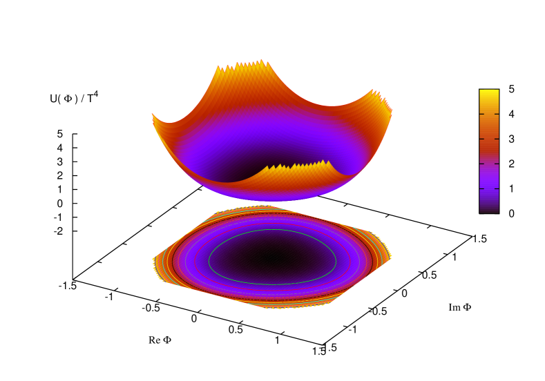
$T=1$ GeV $>T_{0}$

“Color deconfinement”

$\left\langle\Phi\right\rangle\neq 0\longrightarrow$ breaking of $\mathbb{Z}_{3}$

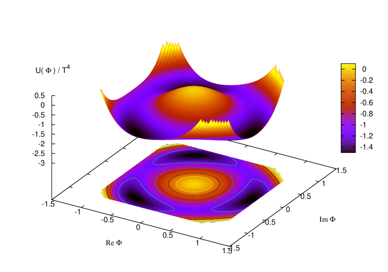
Figure 1: Effective potential in the pure gauge sector (Eq. (6)) for two characteristic temperatures, below and above the critical temperature $T_{0}$. One can see three minima appearing above $T_{0}$.

II.3 Coupling between quarks and the gauge sector: the PNJL model

In the presence of dynamical quarks the $\mathbb{Z}_{3}$ symmetry is explicitly broken. One cannot rigorously talk of a phase transition, but the expectation value of the Polyakov loop still serves as an indicator for the crossover between the phase where color confinement occurs ($\Phi\longrightarrow 0$) and the one where color is deconfined ($\Phi\longrightarrow 1$).

The PNJL model attempts to describe in a simple way the two characteristic phenomena of QCD, namely deconfinement and chiral symmetry breaking.

In order to describe the coupling of quarks to the chiral condensate, we start from an NJL description of quarks (global $SU_{c}(3)$ symmetric point-like interaction), coupled in a minimal way to the Polyakov loop, via the following Lagrangian (Ratti:2005jh ):

$$\mathcal{L}_{PNJL}=\bar{q}\left(i\gamma_{\mu}D^{\mu}-\hat{m}_{0}\right)q+G_{1}\left[\left(\bar{q}q\right)^{2}+\left(\bar{q}i\gamma_{5}\vec{\tau}q\right)^{2}\right]-\mathcal{U}\left(\Phi[A],\bar{\Phi}[A];T\right),$$ (8)

where the covariant derivative reads $D^{\mu}=\partial^{\mu}-iA^{\mu}$ and $A^{\mu}=\delta^{\mu}_{0}A^{0}$ (Polyakov gauge), with $A^{0}=-iA_{4}$. The strong coupling constant $g_{S}$ is absorbed in the definition of $A^{\mu}(x)=g_{S}{\cal A}^{\mu}_{a}(x)\frac{\lambda_{a}}{2}$ where ${\cal A}^{\mu}_{a}$ is the gauge field ($SU_{c}(3)$) and $\lambda_{a}$ are the Gell–Mann matrices. We notice explicitly that at $T=0$ the Polyakov loop and the quark sector decouple.

In order to address the finite density case, it turns out to be useful to introduce the following effective Lagrangian:

$$\mathcal{L}^{\prime}_{PNJL}=\mathcal{L}_{PNJL}+\mu\bar{q}\gamma^{0}q\;,$$ (9)

which leads to the customary grand canonical Hamiltonian. In the above the chemical potential term accounts for baryon number conservation which, in the grand canonical ensemble, is not imposed exactly, but only through its expectation value. Let us comment here the range of applicability of the PNJL model. As already stated in Ref. Ratti:2005jh , in the PNJL model the gluon dynamics is reduced to a chiral-point coupling between quarks together with a simple static background field representing the Polyakov loop. This picture cannot be expected to work outside a limited range of temperatures. At large temperatures transverse gluons are known to be thermodynamically active degrees of freedom: they are not taken into account in the PNJL model. Hence based on the conclusions drawn in Meisinger:2003id according to which transverse gluons start to contribute significantly for $T>2.5\,T_{c}$, we can assume that the range of applicability of the model is limited roughly to $T\leq(2-3)T_{c}$.

II.4 Field equations

II.4.1 Hartree approximation

In this Section we derive the gap equation in the Hartree approximation, whose solution provides the self-consistent PNJL mass of the dressed quark.

We start from the effective lagrangian given in Eq. (9). The imaginary time formalism is employed. One defines the vertices $\Gamma_{M}$, where $M=\{S,P\}$, in the scalar ($\Gamma_{S}\equiv\mathbb{I}$) and pseudo-scalar ($\Gamma_{P}^{a}\equiv i\gamma_{5}\tau^{a}$) channel. The diagrammatic Hartree equation reads:

$$\begin{minipage}[c]{34.14322pt} \includegraphics[width=34.14322pt]{g} \end{minipage}=\begin{minipage}[c]{34.14322pt} \includegraphics[width=34.14322pt]{g0} \end{minipage}+\begin{minipage}[c]{34.14322pt} \includegraphics[width=34.14322pt]{g0} \end{minipage}\begin{minipage}[c]{34.14322pt} \includegraphics[width=34.14322pt]{Sigma} \end{minipage}\begin{minipage}[c]{34.14322pt} \includegraphics[width=34.14322pt]{g} \end{minipage}=\begin{minipage}[c]{34.14322pt} \includegraphics[width=34.14322pt]{g0} \end{minipage}+\includegraphics[width=102.43008pt,origin=B]{G0SigmaHG}$$ (10)

where the thin line denotes the free propagator in the constant (we work in the mean field) background field $A_{4}$: $S_{0}(p)=\begin{minipage}[c]{19.91684pt} \includegraphics[width=19.91684pt]{g0} \end{minipage}=-({p/}-m_{0}+\gamma^{0}(\mu-iA_{4}))^{-1}$, the thick line the Hartree propagator $S(p)=\begin{minipage}[c]{19.91684pt} \includegraphics[width=19.91684pt]{g} \end{minipage}=-({p/}-m+\gamma^{0}(\mu-iA_{4}))^{-1}$, the cross ( ) the vertex $\Gamma_{M}$ and the dot ( ) represents $2G_{1}$, the coupling constant in the scalar-pseudoscalar channel (indeed due to parity invariance only the scalar vertex contributes).
Besides, $\begin{minipage}[c]{42.67912pt} \includegraphics[width=42.67912pt]{Sigma} \end{minipage}=\begin{minipage}[c]{28.45274pt} \includegraphics[width=28.45274pt]{SigmaH} \end{minipage}$ is the Hartree self-energy and $m\equiv m_{0}+\Sigma$. The Hartree equation then reads:

$$m-m_{0}=2G_{1}T\ \mathrm{Tr}\sum_{n=-\infty}^{+\infty}\int_{\Lambda}\frac{\mathrm{d}^{3}p}{\left(2\pi\right)^{3}}\frac{-1}{{p/}-m+\gamma^{0}(\mu-iA_{4})}$$ (11)

In all the above formulas, $p_{0}=i\omega_{n}$ and $\omega_{n}=(2n+1)\pi T$ is the Matsubara frequency for a fermion; the trace is taken over color, Dirac and flavor indices. The symbol $\int_{\Lambda}$ denotes the three dimensional momentum regularisation; we use an ultraviolet cut-off $\Lambda$ for both the zero and the finite temperature contributions. Our choice is motivated by our wish to discuss mesonic properties driven by chiral symmetry considerations, a feature not well described if one only regularizes the $T=0$ part (in particular in the vector sector the Weinberg sum rule is not well satisfied). Through a convenient gauge transformation of the Polyakov line, the background field $A_{4}$ in Eq. (11) can always be put in a diagonal form. This allows one to straightforwardly perform the sum over the Matsubara frequencies yielding (see also section III.3):

$$m-m_{0}=2G_{1}N_{f}\sum_{i=1}^{N_{c}}\int_{\Lambda}\frac{\mathrm{d}^{3}p}{\left(2\pi\right)^{3}}\frac{2m}{E_{p}}[1-f(E_{p}-\mu+iA_{4}^{ii})-f(E_{p}+\mu-iA_{4}^{ii})]\,.$$ (12)

By introducing the modified distribution functions $f^{+}_{\Phi}$ and $f^{-}_{\Phi}$, here derived for $N_{c}=3$ (with the usual notation $\beta=1/T$):

$$f^{+}_{\Phi}(E_{p}) = \frac{\left(\Phi+2\bar{\Phi}e^{-\beta\left(E_{p}-\mu\right)}\right)e^{-\beta\left(E_{p}-\mu\right)}+e^{-3\beta\left(E_{p}-\mu\right)}}{1+3\left(\Phi+\bar{\Phi}e^{-\beta\left(E_{p}-\mu\right)}\right)e^{-\beta\left(E_{p}-\mu\right)}+e^{-3\beta\left(E_{p}-\mu\right)}}$$ (13)

$$f^{-}_{\Phi}(E_{p}) = \frac{\left(\bar{\Phi}+2\Phi e^{-\beta\left(E_{p}+\mu\right)}\right)e^{-\beta\left(E_{p}+\mu\right)}+e^{-3\beta\left(E_{p}+\mu\right)}}{1+3\left(\Phi+\bar{\Phi}e^{-\beta\left(E_{p}+\mu\right)}\right)e^{-\beta\left(E_{p}+\mu\right)}+e^{-3\beta\left(E_{p}+\mu\right)}},$$ (14)

the gap equation reads:

$$m-m_{0}=2G_{1}N_{f}N_{c}\int_{\Lambda}\frac{\mathrm{d}^{3}p}{\left(2\pi\right)^{3}}\frac{2m}{E_{p}}[1-f^{+}_{\Phi}(E_{p})-f^{-}_{\Phi}(E_{p})]\,.$$ (15)

The latter is valid for any $N_{c}$ providing one uses the corresponding $f^{+,-}_{\Phi}$. Notice that Eq. (11), after computing the trace on Dirac and isospin indices, can be viewed as a generalization of the corresponding zero temperature and density NJL gap equation

$$m-m_{0} = 8iG_{1}mN_{c}N_{f}\int_{\Lambda}\frac{d^{4}p}{(2\pi)^{4}}\frac{1}{p^{2}-m^{2}},$$ (16)

after adopting the following symbolic replacements:

$$p=(p_{0},\vec{p}) \rightarrow (i\omega_{n}+\mu-iA_{4},\vec{p})$$ (17)

$$i\int_{\Lambda}\frac{d^{4}p}{(2\pi)^{4}} \rightarrow -T\frac{1}{N_{c}}\mathrm{Tr}_{c}\sum_{n}\int_{\Lambda}\frac{d^{3}p}{(2\pi)^{3}},$$ (18)

II.4.2 Grand potential at finite temperature and density in Hartree approximation

The usual techniques Klevansky:1992qe ; Schwarz:1999dj can be used to obtain the PNJL grand potential from the Hartree propagator (see Ratti:2005jh ):

$$\Omega=\Omega(\Phi,\bar{\Phi},m;T,\mu) = {\cal U}\left(\Phi,\bar{\Phi},T\right)+\frac{(m-m_{0})^{2}}{4G_{1}}-2N_{c}N_{f}\int_{\Lambda}\frac{\mathrm{d}^{3}p}{\left(2\pi\right)^{3}}\,{E_{p}}$$

$$-2N_{f}\,T\int_{\Lambda}\frac{\mathrm{d}^{3}p}{\left(2\pi\right)^{3}}\left\{\mathrm{Tr}_{c}\ln\left[1+L^{\dagger}\mathrm{e}^{-\left(E_{p}-\mu\right)/T}\right]+\mathrm{Tr}_{c}\ln\left[1+L\mathrm{e}^{-\left(E_{p}+\mu\right)/T}\right]\right\}\leavevmode\nobreak\ .$$

In the above formula $E_{p}=\sqrt{\vec{p}\,^{2}+m^{2}}$ is the Hartree single quasi-particle energy (which includes the constituent quark mass). We then define $z^{+,-}_{\Phi}$ and compute them for $N_{c}=3$:

$$z^{+}_{\Phi}\equiv\mathrm{Tr}_{c}\ln\left[1+L^{\dagger}\mathrm{e}^{-\left(E_{p}-\mu\right)/T}\right] = \ln\left\{1+3\left(\bar{\Phi}+\Phi e^{-\left(E_{p}-\mu\right)/T}\right)e^{-\left(E_{p}-\mu\right)/T}+e^{-3\left(E_{p}-\mu\right)/T}\right\}\$$ (20)

$$z^{-}_{\Phi}\equiv\mathrm{Tr}_{c}\ln\left[1+L\mathrm{e}^{-\left(E_{p}+\mu\right)/T}\right] = \ln\left\{1+3\left(\Phi+\bar{\Phi}e^{-\left(E_{p}+\mu\right)/T}\right)e^{-\left(E_{p}+\mu\right)/T}+e^{-3\left(E_{p}+\mu\right)/T}\right\}\leavevmode\nobreak\ .\$$ (21)

II.5 Mean field results

The solutions of the mean field equations are obtained by minimizing the grand potential with respect to $m$, $\Phi$ and $\bar{\Phi}$, namely (again below $N_{c}=3$)

$$\frac{\partial\Omega}{\partial\Phi} = 0$$ (22)

$$= \frac{T^{4}}{2}(-b_{2}(T)\bar{\Phi}-b_{3}\Phi^{2}+b_{4}\Phi\bar{\Phi}^{2})$$

$$-6N_{f}T\int_{\Lambda}\frac{\mathrm{d}^{3}p}{\left(2\pi\right)^{3}}\left\{\frac{e^{-2(E_{p}-\mu)/T}}{1+3\left(\bar{\Phi}+\Phi e^{-\left(E_{p}-\mu\right)/T}\right)e^{-\left(E_{p}-\mu\right)/T}+e^{-3\left(E_{p}-\mu\right)/T}}\right.$$

$$\qquad\qquad\left.+\frac{e^{-(E_{p}+\mu)/T}}{1+3\left(\Phi+\bar{\Phi}e^{-\left(E_{p}+\mu\right)/T}\right)e^{-\left(E_{p}+\mu\right)/T}+e^{-3\left(E_{p}+\mu\right)/T}}\right\},$$

$$\frac{\partial\Omega}{\partial\bar{\Phi}} = 0$$ (23)

$$= \frac{T^{4}}{2}(-b_{2}(T)\Phi-b_{3}\bar{\Phi}^{2}+b_{4}\bar{\Phi}\Phi^{2})$$

$$-6N_{f}T\int_{\Lambda}\frac{\mathrm{d}^{3}p}{\left(2\pi\right)^{3}}\left\{\frac{e^{-(E_{p}-\mu)/T}}{1+3\left(\bar{\Phi}+\Phi e^{-\left(E_{p}-\mu\right)/T}\right)e^{-\left(E_{p}-\mu\right)/T}+e^{-3\left(E_{p}-\mu\right)/T}}\right.$$

$$\qquad\qquad\left.+\frac{e^{-2(E_{p}+\mu)/T}}{1+3\left(\Phi+\bar{\Phi}e^{-\left(E_{p}+\mu\right)/T}\right)e^{-\left(E_{p}+\mu\right)/T}+e^{-3\left(E_{p}+\mu\right)/T}}\right\}$$

and

$$\frac{\partial\Omega}{\partial m} = 0$$ (24)

which coincides with the gap equation (11). A complete discussion of the results in mean field approximation is given in Ratti:2005jh . For the purpose of this article, we only briefly discuss the result obtained in Ratti:2005jh for the net quark number density, defined by the equation

$$\frac{n_{q}\left(T,\mu\right)}{T^{3}}=-\frac{1}{T^{3}}\frac{\partial\Omega\left(T,\mu\right)}{\partial\mu},$$ (25)

that we display in Fig. 2. Note that an implicit $\mu$-dependence of $\Omega$ is also contained in the effective quark mass $m$ and in the expectation values $\Phi$ and $\bar{\Phi}$. Nevertheless, due to stationary equations (22, 23, 24), only the explicit dependence arising from the statistical factors has to be differentiated.

One can see that the NJL model (corresponding to the $\Phi\to 1$ limit of PNJL) badly fails in reproducing the lattice findings, while the PNJL results provide a good approximation for them. One realizes that, at a given value of $T$ and $\mu$, the NJL model always overestimates the baryon density, even if, for large temperatures, when in PNJL $\Phi\to 1$, the two models merge.

On the other hand in the PNJL model below $T_{c}$ (when $\Phi,\bar{\Phi}\to 0$) one can see from Eqs. (20) and (21) that contributions coming from one and two (anti-)quarks are frozen, due to their coupling with $\Phi$ and $\bar{\Phi}$, while three (anti-)quark contributions are not suppressed even below $T_{c}$. This implies that, at fixed values of $T$ and $\mu$, the PNJL value for $n_{q}$ results much lower than in the NJL case. In fact all the possible contributions to the latter turn out to be somehow suppressed: the one- and two-quark contributions because of $\Phi,\bar{\Phi}\to 0$, while the thermal excitation of three quark clusters has a negligible Boltzmann factor.

One would be tempted to identify these clusters of three dressed (anti-)quarks with precursors of (anti-)baryons. Indeed no binding for these structures is provided by the model. In any case it is encouraging that coupling the NJL Lagrangian with the Polyakov loop field leads to results pointing into the right direction.

In the following Section we explore the PNJL results in the mesonic sector, investigating whether coupling the (anti-)quarks with the $\Phi$ field constrains the dressed $q\bar{q}$ pairs to form stable colorless structures.

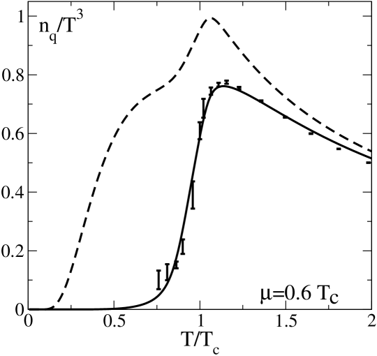
Figure 2: PNJL (solid line), NJL (dotted line) and lattice results (points) for the net quark density at $\mu=0.6T_{c}$ (from Ratti:2005jh ).

III Mesonic correlators

In this Section, we address the central topic of our paper, i.e. the study of correlators of current operators carrying the quantum numbers of physical mesons. We focus our attention on two particular cases: the pseudoscalar iso-vector current

$${J_{P}}^{a}(x) = \bar{q}(x)i\gamma_{5}\tau^{a}q(x)\quad\mbox{ (pion)}$$ (26)

and the scalar iso-scalar current:

$${J_{S}}(x) = \bar{q}(x)q(x)-\langle\bar{q}(x)q(x)\rangle\quad\mbox{ (sigma)}.$$ (27)

These are in fact the channels of interest to study the chiral symmetry breaking-restoration pattern. In particular the scalar current represents the fluctuations of the order parameter.

In terms of the above currents, the following mesonic correlation functions and their Fourier transforms are defined:

$$C^{PP}_{ab}(q^{2})\equiv i\int d^{4}xe^{iq.x}\left\langle 0\left|T\left(J^{a}_{P}(x)J^{b\dagger}_{P}(0)\right)\right|0\right\rangle=C^{PP}(q^{2})\delta_{ab}$$ (28)

and

$$C^{SS}(q^{2})\equiv i\int d^{4}xe^{iq.x}\left\langle 0\left|T\left(J_{S}(x)J^{\dagger}_{S}(0)\right)\right|0\right\rangle.$$ (29)

In the above equations, the expectation value is taken with respect to the vacuum state and $T$ is the time-ordered product.

III.1 Schwinger – Dyson equations at $\boldsymbol{T=\mu=0}$

Here we briefly summarize the usual NJL results for the mesonic correlators Oertel:2000jp ; Klevansky:1997dk ; Schulze:1994fy ; Davidson:1995fq , which we are going to generalize in Sec. (III.3) by including the case in which quarks propagate in the temporal background gauge field related to the Polyakov loop. The Schwinger – Dyson equation for the meson correlator $C^{MM}$ is solved in the ring approximation (RPA):

$$C^{MM}(q^{2}) = \Pi^{MM}(q^{2})+\sum_{M^{\prime}}\Pi^{MM^{\prime}}(2G_{1})C^{M^{\prime}M}$$ (30)

where the

$$\Pi^{MM^{\prime}} \equiv \int_{\Lambda}\frac{d^{4}p}{(2\pi)^{4}}\mathrm{Tr}\left(\Gamma_{M}S(p+q)\Gamma_{M^{\prime}}S(q)\right)$$ (31)

are the one loop polarizations and $S(p)$ is the Hartree quark propagator. In terms of diagrams, one defines:

$$\Pi^{MM^{\prime}} = \Gamma_{M}\begin{minipage}[c]{71.13188pt} \includegraphics[width=71.13188pt]{Pi} \end{minipage}\Gamma_{M^{\prime}}$$ (32)

and

$$C^{MM} = \begin{minipage}[c]{56.9055pt} \includegraphics[width=56.9055pt]{c} \end{minipage}=\begin{minipage}[c]{56.9055pt} \includegraphics[width=56.9055pt]{PPi} \end{minipage}+\begin{minipage}[c]{113.81102pt} \includegraphics[width=113.81102pt]{PiC} \end{minipage}.$$ (33)

Hence, we need the following (one loop) polarization functions:

$$\Pi^{PP}_{ab}(q^{2}) = \int_{\Lambda}\frac{d^{4}p}{(2\pi)^{4}}\mathrm{Tr}\left(i\gamma_{5}\tau^{a}S(p+q)i\gamma_{5}\tau^{b}S(q)\right)=\Pi^{PP}(q^{2})\delta_{ab}$$ (34)

$$\Pi^{SS}(q^{2}) = \int_{\Lambda}\frac{d^{4}p}{(2\pi)^{4}}\mathrm{Tr}\left(S(p+q)S(q)\right).$$ (35)

Thus, for example, for the pion channel:

$$\Pi^{PP}(q^{2}) = -4iN_{c}N_{f}\int_{\Lambda}\frac{d^{4}p}{(2\pi)^{4}}\frac{m^{2}-p^{2}+q^{2}/4}{[(p+q/2)^{2}-m^{2}][(p-q/2)^{2}-m^{2}]}$$

$$= 4iN_{c}N_{f}I_{1}-2iN_{c}N_{f}q^{2}I_{2}(q^{2})$$

the loop integrals being:

$$I_{1} = \int_{\Lambda}\frac{d^{4}p}{(2\pi)^{4}}\frac{1}{p^{2}-m^{2}}$$ (37)

$$I_{2}(q^{2}) = \int_{\Lambda}\frac{d^{4}p}{(2\pi)^{4}}\frac{1}{\left[(p+q)^{2}-m^{2}\right]\left[p^{2}-m^{2}\right]}.$$ (38)

By defining:

$$f^{2}_{P}(q^{2}) = -4iN_{c}m^{2}I_{2}(q^{2})$$ (39)

and owing to the fact that the Hartree equation (16) implies

$$I_{1} = \frac{m-m_{0}}{8iG_{1}mN_{c}N_{f}},$$ (40)

one shows that Klevansky:1997dk

$$\Pi^{PP}(q^{2}) = \frac{m-m_{0}}{2G_{1}m}+f^{2}_{P}(q^{2})\frac{q^{2}}{m^{2}}$$ (41)

$$\Pi^{SS}(q^{2}) = \frac{m-m_{0}}{2G_{1}m}+f^{2}_{P}(q^{2})\frac{q^{2}-4m^{2}}{m^{2}}.$$ (42)

The explicit solutions of the Schwinger–Dyson equations in ring approximation then read:

• Scalar iso-scalar sector

  $$C^{SS}(q^{2}) = \Pi^{SS}(q^{2})+\Pi^{SS}(q^{2})(2G_{1})C^{SS}(q^{2})$$ (43)

  $$\Rightarrow C^{SS} = \frac{\Pi^{SS}(q^{2})}{1-2G_{1}\Pi^{SS}(q^{2})}.$$ (44)

• Pseudo-scalar iso-vector sector

  $$C^{PP}(q^{2}) = \Pi^{PP}(q^{2})+\Pi^{PP}(q^{2})(2G_{1})C^{PP}(q^{2})$$ (45)

  $$\Rightarrow C^{PP} = \frac{\Pi^{PP}(q^{2})}{1-2G_{1}\Pi^{PP}(q^{2})}.$$ (46)

III.2 NJL Schwinger-Dyson equations at finite $T$ and $\mu$

In order to study the problem at finite temperature and baryon density in the imaginary time formalism ($t=-i\tau$ with $\tau\in[0,\beta]$), the $\tau$-ordered product of the operators replaces the usual time-ordering and all the expectation values are taken over the grand-canonical ensemble.

One can decompose all the integrands, for example in $I_{2}$, as a sum of partial fractions of the form

$$\frac{1}{i\omega_{n}-E+\mu}.$$ (47)

The sum over Matsubara frequencies is then computed by using:

$$\frac{1}{\beta}\sum_{n}\frac{1}{i\omega_{n}-E+\mu}=f(E-\mu)$$ (48)

where the Fermi – Dirac distribution function is given by:

$$f(E)=\frac{1}{1+e^{\beta E}}.$$ (49)

The integrals $I_{1}$ and $I_{2}$ (Eqs. (37) and (38)) at finite temperature and density are then expressed as Oertel:2000jp ; Hatsuda:1986gu ; Florkowski:1993br ; Su:1990dy ; Farias:2004tf :

$$I_{1} = -i\int_{\Lambda}\frac{d^{3}p}{(2\pi)^{3}}\frac{1-f(E_{p}-\mu)-f(E_{p}+\mu)}{2E_{p}}$$ (50)

$$I_{2}(\omega,\vec{q}) = i\int_{\Lambda}\frac{d^{3}p}{(2\pi)^{3}}\frac{1}{2E_{p}2E_{p+q}}\frac{f(E_{p}+\mu)+f(E_{p}-\mu)-f(E_{p+q}+\mu)-f(E_{p+q}-\mu)}{\omega-E_{p+q}+E_{p}}$$ (51)

$$+i\int_{\Lambda}\frac{d^{3}p}{(2\pi)^{3}}\frac{1-f(E_{p}-\mu)-f(E_{p+q}+\mu)}{2E_{p}2E_{p+q}}\left(\frac{1}{\omega+E_{p+q}+E_{p}}-\frac{1}{\omega-E_{p+q}-E_{p}}\right)$$

(these expression are implicitly taken at $\omega\rightarrow\omega+i\eta$ to obtain retarded correlation functions).

Then all the zero temperature results can be continued to finite temperature and density by a redefinition of $I_{1}$ and $I_{2}$.

At $\vec{q}=\vec{0}$, the integral $I_{2}$ reduces to:

$$I_{2}\left(\omega,\vec{0}\right)=-i\int_{\Lambda}\frac{d^{3}p}{(2\pi)^{3}}\frac{1-f(E_{p}+\mu)-f(E_{p}-\mu)}{E_{p}\left(\omega^{2}-4E_{p}^{2}\right)}$$ (52)

so that we obtain:

$$\Pi^{PP}\left(\omega,\vec{0}\right) = -8N_{c}N_{f}\int_{\Lambda}\frac{d^{3}p}{(2\pi)^{3}}\frac{E_{p}}{\omega^{2}-4E_{p}^{2}}\left(1-f(E_{p}+\mu)-f(E_{p}-\mu)\right)$$ (53)

$$\Pi^{SS}\left(\omega,\vec{0}\right) = -8N_{c}N_{f}\int_{\Lambda}\frac{d^{3}p}{(2\pi)^{3}}\frac{1}{E_{p}}\frac{E_{p}^{2}-m^{2}}{\omega^{2}-4E_{p}^{2}}\left(1-f(E_{p}+\mu)-f(E_{p}-\mu)\right).$$ (54)

It then follows:

$$\Im m\,\left(-iI_{2}(\omega,0)\right) = \frac{1}{16\pi}\left(1-f\left(\frac{\omega}{2}-\mu\right)-f\left(\frac{\omega}{2}+\mu\right)\right)\sqrt{\frac{\omega^{2}-4m^{2}}{\omega^{2}}}$$ (55)

$$\times\Theta(\omega^{2}-4m^{2})\Theta(4(\Lambda^{2}+m^{2})-\omega^{2})$$

(and of course, the real part is given by the Cauchy principal value of the integral). Hence:

$$\Im m\,\Pi^{PP}(\omega,0)=2N_{f}N_{c}\omega^{2}\Im m\,(-iI_{2}(\omega))$$

$$\qquad=\frac{N_{c}N_{f}\omega^{2}}{8\pi}\sqrt{\frac{\omega^{2}-4m^{2}}{\omega^{2}}}\,N(\omega,\mu)\,\Theta(\omega^{2}-4m^{2})\Theta(4(\Lambda^{2}+m^{2})-\omega^{2})$$ (56)

$$\Im m\,\Pi^{SS}(\omega,0)=$$

$$=\frac{N_{c}N_{f}(\omega^{2}-4m^{2})}{8\pi}\sqrt{\frac{\omega^{2}-4m^{2}}{\omega^{2}}}\,N(\omega,\mu)\,\Theta(\omega^{2}-4m^{2})\Theta(4(\Lambda^{2}+m^{2})-\omega^{2})$$

(57)

with

$$N(\omega,\mu)=\left(1-f\left(\frac{\omega}{2}-\mu\right)-f\left(\frac{\omega}{2}+\mu\right)\right).$$ (58)

III.3 PNJL Schwinger-Dyson equations at finite $\boldsymbol{T}$ and $\boldsymbol{\mu}$

Here we derived explicitly the expressions for the modified Fermi–Dirac distribution functions Eqs.(13) and (14).

Again, all the summation over Matsubara frequencies can be reduced to the sum of fractions like (47). By defining:

$$F(E_{p}-\mu+iA_{4}) \equiv \frac{1}{\beta}\sum_{n}\frac{1}{i\omega_{n}-E_{p}+\mu-iA_{4}}$$ (59)

one shows that:

$$\mathrm{Tr}_{c}F(E_{p}-\mu+iA_{4})$$

$$\qquad=f(E_{p}-\mu+i(A_{4})_{11})+f(E_{p}-\mu+i(A_{4})_{22})+f(E_{p}-\mu+i(A_{4})_{33})$$ (60)

where $(A_{4})_{ii}$ are the elements of the diagonalized $A_{4}$ matrix.

Let us write the Fermi–Dirac distribution function according to:

$$f(E_{p}-\mu) \equiv -\frac{1}{\beta}\frac{\partial z^{+}}{\partial E_{p}}\;,$$ (61)

where

$$z^{+} \equiv \ln\left(1+e^{-\beta\left(E_{p}-\mu\right)}\right)$$ (62)

can be viewed as a density of partition function. We then obtain

$$\mathrm{Tr}_{c}F(E_{p}-\mu+iA_{4}) = -\frac{1}{\beta}\sum_{i}\frac{\partial\ln\left(1+e^{-\beta\left(E_{p}-\mu\right)}e^{-i\beta(A_{4})_{ii}}\right)}{\partial E_{p}}=-\frac{1}{\beta}\,\mathrm{Tr}_{c}\frac{\partial\ln\left(1+e^{-\beta\left(E_{p}-\mu\right)}e^{-i\beta A_{4}}\right)}{\partial E_{p}}$$ (63)

$$= -\frac{1}{\beta}\,\mathrm{Tr}_{c}\frac{\partial\ln\left(1+L^{\dagger}e^{-\beta\left(E_{p}-\mu\right)}\right)}{\partial E_{p}}=-\frac{1}{\beta}\,\frac{\partial z_{\Phi}^{+}}{\partial E_{p}}$$

where $z_{\Phi}^{+}=\ln\left(1+L^{\dagger}e^{-\beta\left(E_{p}-\mu\right)}\right)$ is the corresponding density of partition function in PNJL (already introduced in Eq.(20)). Hence

$$\mathrm{Tr}_{c}F(E_{p}-\mu+iA_{4}) = 3\frac{\left(\bar{\Phi}+2\Phi e^{-\beta\left(E_{p}-\mu\right)}\right)e^{-\beta\left(E_{p}-\mu\right)}+e^{-3\beta\left(E_{p}-\mu\right)}}{1+3\left(\bar{\Phi}+\Phi e^{-\beta\left(E_{p}-\mu\right)}\right)e^{-\beta\left(E_{p}-\mu\right)}+e^{-3\beta\left(E_{p}-\mu\right)}}.$$ (64)

We can do the same for the $F(E_{p}+\mu-iA_{4})$ case.

Hence, we can define:

$$f^{+}_{\Phi}(E_{p}) \equiv \frac{1}{N_{c}}\mathrm{Tr}_{c}F(E_{p}-\mu+iA_{4})=-\frac{1}{\beta N_{c}}\frac{\partial z_{\Phi}^{+}}{\partial E_{p}}$$ (65)

and

$$f^{-}_{\Phi}(E_{p}) \equiv \frac{1}{N_{c}}\mathrm{Tr}_{c}F(E_{p}+\mu-iA_{4})=-\frac{1}{\beta N_{c}}\frac{\partial z_{\Phi}^{-}}{\partial E_{p}}\;,$$ (66)

where $z_{\Phi}^{+}$ and $z_{\Phi}^{-}$ are the densities (20) and (21) of the partition function in PNJL.

The only changes in going from NJL to PNJL can then be summarized in the following prescriptions:

$$f(E_{p}-\mu) \Longrightarrow f^{+}_{\Phi}(E_{p})=\frac{\left(\bar{\Phi}+2\Phi e^{-\beta\left(E_{p}-\mu\right)}\right)e^{-\beta\left(E_{p}-\mu\right)}+e^{-3\beta\left(E_{p}-\mu\right)}}{1+3\left(\bar{\Phi}+\Phi e^{-\beta\left(E_{p}-\mu\right)}\right)e^{-\beta\left(E_{p}-\mu\right)}+e^{-3\beta\left(E_{p}-\mu\right)}}$$ (67)

$$f(E_{p}+\mu) \Longrightarrow f^{-}_{\Phi}(E_{p})=\frac{\left(\Phi+2\bar{\Phi}e^{-\beta\left(E_{p}+\mu\right)}\right)e^{-\beta\left(E_{p}+\mu\right)}+e^{-3\beta\left(E_{p}+\mu\right)}}{1+3\left(\Phi+\bar{\Phi}e^{-\beta\left(E_{p}+\mu\right)}\right)e^{-\beta\left(E_{p}+\mu\right)}+e^{-3\beta\left(E_{p}+\mu\right)}}.$$ (68)

Of course in the above the corresponding PNJL quark mass $m$, given by the Hartree equation with these modified distribution functions, should be used.

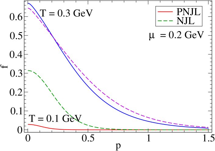
Figure 3: Fermi – Dirac distribution function $f(E_{p}-\mu)$ (valid for the NJL model) and the corresponding function $f^{+}_{\Phi}(E_{p})$ (valid for the PNJL one) as functions of $p$, for different temperatures. $\Phi$, $\bar{\Phi}$ and m are taken at their mean field values. The upper lines refer to $T=0.3$ GeV, the lower ones to $T=0.1$ GeV.

The functions $f(E_{p}-\mu)$ and $f^{+}_{\Phi}(E_{p})$ are displayed in Fig. 3 for two different temperatures versus $p$, keeping $\Phi$, $\bar{\Phi}$ and $m$ at the mean field values. For temperatures smaller than $T_{c}$ (for example $T=0.1$ GeV $\simeq T_{c}/2$), the effect of the Polyakov loop turns out to be more relevant than for larger temperatures, close to $T_{c}$.

In discussing the PNJL results for the net quark density we already stressed the role of $\Phi$ and $\bar{\Phi}$ in suppressing one and two (anti-)quark clusters in the confined phase. This also emerges in Fig. 3 comparing the PNJL and NJL curves at $T=0.1$ GeV. Clearly the two models differ substantially when $\Phi,\bar{\Phi}\to 0$. On the contrary, as $\Phi,\bar{\Phi}\to 1$ they lead to similar results.

We conclude this Section by stressing once more that the recipes given in Eqs. (67) and (68) allow one to straightforwardly generalize NJL results to the PNJL case.

IV Meson spectral function and propagator

In the rest of the paper we present our numerical results for the masses and spectral functions of the scalar ($\sigma$) and pseudoscalar ($\pi$) mesons in a hot and dense environment.

The spectral (or strength) function $F^{MM}$ of the correlator $C^{MM}$ is defined according to:

$$F^{MM}(\omega,\vec{q})\equiv\Im m\,C^{MM}(\omega+i\eta,\vec{q})=\Im m\,\frac{\Pi^{MM}(\omega+i\eta,\vec{q})}{1-2G_{1}\Pi^{MM}(\omega+i\eta,\vec{q})}.$$ (69)

For the sake of simplicity, in the following we will consider only the zero momentum case: hence we will drop the dependence on $\vec{q}$. One gets:

$$F^{MM}(\omega)=\frac{\pi}{2G_{1}}\frac{1}{\pi}\frac{2G_{1}\Im m\,\Pi^{MM}(\omega+i\eta)}{\left(1-2G_{1}\Re e\,\Pi^{MM}(\omega)\right)^{2}+\left(2G_{1}\Im m\,\Pi^{MM}(\omega+i\eta)\right)^{2}}.$$ (70)

For $\omega<2m(T,\mu)$, $\Im m\,\Pi=0$ hence the decay channel into a dressed $q\bar{q}$ pair is closed and the spectral function gets a bound state contribution expressed by a delta peak in correspondence of the mass of the meson. Indeed:

$$F^{MM}(\omega)=\frac{\pi}{2G_{1}}\delta\left(1-2G_{1}\Re e\,{\Pi^{MM}}(\omega)\right)=\frac{\pi}{4G_{1}^{2}{\left|\frac{\partial\Re e\,{\Pi^{MM}}}{\partial\omega}\right|}_{\omega=m_{M}}}\delta(\omega-m_{M})\;.$$ (71)

and the meson mass $m_{M}$ is the solution of the equation

$$1-2G_{1}\Re e\,\Pi^{MM}(m_{M})=0\;.$$ (72)

On the other hand, for $\omega>2m(T,\mu)$, $\Im m\,\Pi\neq 0$ and the meson spectral function gets a continuum contribution. Thus if the solution of Eq. (72) occurs above such a threshold, then the spectral function will still present a peak characterized by a width related to the decay channel $M\to q\bar{q}$. In such a case the meson is no longer a bound, but simply a resonant state. If $\Im m\,\Pi$ stays almost constant around the position of the peak, the spectral function is well approximated by a Lorentzian with a width given by:

$$\Gamma_{M}=2G_{1}\Im m\,\Pi^{MM}(m_{M})\;.$$ (73)

On the other hand, if $\Im m\,\Pi$ varies with $\omega$ the solution of Equation (72) and the maximum of the spectral function no longer coincide, the latter being typically below the former. In the following we choose to identify the mass of the meson with the maximum of the spectral function.

We notice that $C^{MM}$ is a correlator of current operators which is the quantity investigated in lattice calculations. But one can also get useful information concerning $q\bar{q}$ scattering processes by extracting the meson propagator from the $T-$matrix Oertel:2000cw .

In the present framework it can be shown that the propagator for a meson is

$$D_{M}(\omega) = -G_{1}\frac{C^{MM}(\omega)}{\Pi^{MM}(\omega)}.$$ (74)

In the quasi-particle approximation, the above simplifies to:

$$D_{M}(\omega) \simeq \frac{-ig^{2}_{Mqq}}{\omega^{2}-m^{2}_{M}}$$ (75)

where $m^{2}_{M}$ verifies the pole equation (72) and the effective meson$-$quark coupling constant,

$$g^{-2}_{Mqq} = {\left.\frac{\partial\Pi^{MM}}{\partial\omega^{2}}\right|}_{\omega=m_{M}},$$ (76)

is the residue at the pole.

V Numerical results

In this Section we present, in the PNJL model, our numerical results for the properties of the $\sigma$ and $\pi$ mesons in a hot and dense environment.

The special role played by the $\sigma$ spectral function, embodying the correlations among the fluctuations of the order parameter (the chiral condensate), was first pointed out in Hatsuda:1985eb , within the NJL model. In particular, it was shown that in the Wigner (ordered) phase of chiral symmetry the $\sigma$ spectral function (which becomes approximatively degenerate with the $\pi$ one, due to chiral symmetry restoration) displays a pronounced peak, moving to lower frequencies and getting narrower as $T\to T_{c}$ from above. The above excitations, characterizing the regime of temperatures slightly exceeding $T_{c}$, were then identified as soft modes, representing a precursor phenomenon of the phase transition.

We will show in the following that the above qualitative features of the mesonic excitations are preserved, once the coupling with the Polyakov loop field is introduced in the NJL model.

V.1 NJL vs. PNJL: Characteristic temperatures

Before discussing the mesonic properties, we need to identify the characteristic temperatures which separate the different thermodynamic phases in PNJL and NJL. In order to define a “critical” temperature one would like to refer to the order parameters (vanishing in the disordered-symmetric phase and non-vanishing in the ordered-broken phase). The latter, as already pointed out, can be identified with the Polyakov loop $\Phi$ (if $m_{q}\to\infty$) and with the chiral condensate $\langle\bar{q}q\rangle$ (if $m_{q}\to 0$), for the deconfinement and chiral phase transitions, respectively. Chiral symmetry restoration is also signalled by $m_{\pi}=m_{\sigma}$ (or, strictly speaking, by the merging of $\pi$ and $\sigma$ spectral functions).

In the present context, chiral symmetry is explicitly broken by the presence of a finite bare quark mass; nevertheless the discontinuity displayed by the order parameter or by its derivatives still allows one to define a critical line in the $(\mu-T)$ plane separating the two phases: for small values of the baryo-chemical potential the transition is known to be a continuous one (cross-over) but for larger densities it becomes first order. A critical temperature, identified with the maximum of $-dm/dT$ ($T^{\chi}_{c}$), is then commonly used in the literature: this can be applied both to NJL and PNJL. The PNJL model also displays a similar cross-over for the effective Polyakov loop $\Phi$ (which was shown to occur at a temperature close to $T^{\chi}_{c}$ in Ref. Ratti:2005jh ). We also notice that, in the low-density limit, two-flavour lattice QCD shows a cross-over, occurring at the same critical temperature both for the deconfinement and the chiral transitions.

A different choice for a common characteristic temperature is also possible, corresponding to the minimum of $m_{\sigma}(T)$ (typical temperature where the pion and sigma spectral functions start to merge); we denote it as $T^{\sigma-min}_{c}$.

In order to compare the NJL and PNJL results, it is useful to follow the evolution of the observables as functions of the temperature, expressed both in physical units (MeV) as well as rescaled in units of a characteristic temperature. For the latter we choose the corresponding $T^{\sigma-min}_{c}$ in NJL and PNJL. Our choice is motivated in Sec. V.4.

These temperatures computed in PNJL and NJL (at $\mu=0$), together with the Mott temperatures for the pion (the temperature at which the decay of a pion into a $\bar{q}q$ pair becomes energetically favourable), are quoted in Table 3. We remind that in the framework of PNJL a further critical temperature related to the deconfinement phase transition can be defined. Its value $T_{c}^{\Phi}=0.250$ GeV corresponds to the $\Phi$ crossover location. Worth noticing is that the value of the latter differs by only $6$ MeV from $T^{\chi}_{c}$. As it is evident from Table 3, the characteristic temperatures that we get in the present approach are much larger than the one which is usually quoted for the chiral/deconfinement phase transition in two flavour QCD ($T_{c}\simeq 173$ MeV) on the basis of lattice calculations. They are also larger than the ones obtained in the PNJL model in Ref. Ratti:2005jh . This difference is due to our choice to regularize both the zero and the finite temperature contributions with a three-dimensional momentum cutoff, and also to the fact that we do not rescale the parameter $T_{0}$ to a smaller value when we introduce quarks in the system. Nevertheless, for the purpose of the present work, the absolute value of the critical temperature is not important: the general properties of mesons that we discuss here are in fact independent of the specific value of $T_{c}$.

PNJL	$T^{\chi}_{c}=0.256$ GeV	$T^{\sigma-min}_{c}=0.277$ GeV	$T_{Mott}=0.272$ GeV $=1.06T^{\chi}_{c}$
NJL	$T^{\chi}_{c}=0.194$ GeV	$T^{\sigma-min}_{c}=0.210$ GeV	$T_{Mott}=0.212$ GeV $=1.09T^{\chi}_{c}$

Table 3: Characteristic temperatures in the NJL and PNJL models at zero chemical potential.

V.2 Mesonic masses and spectral functions

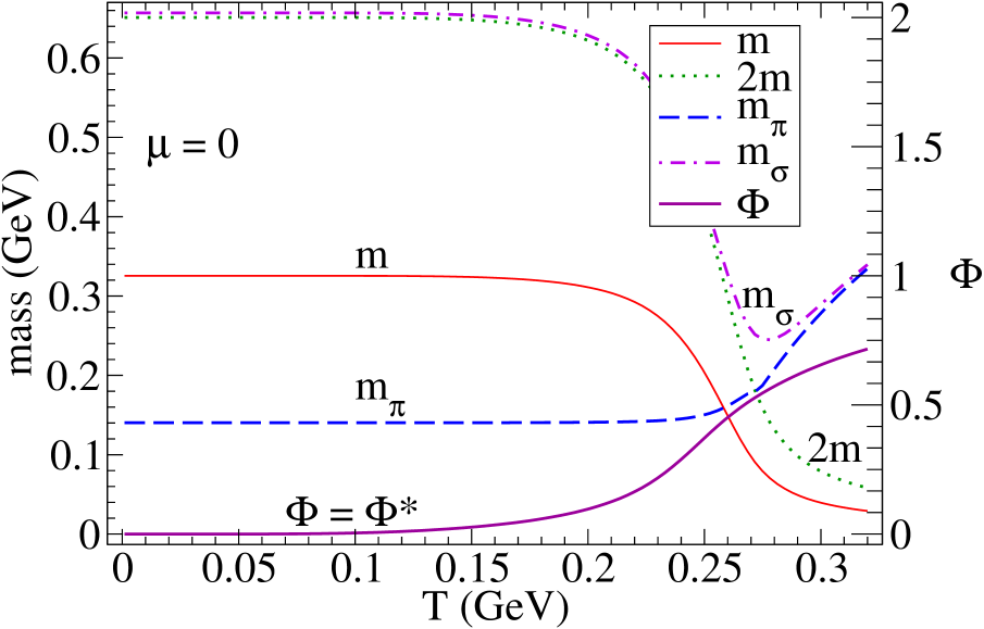
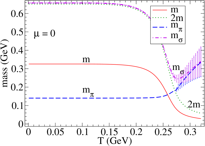
Figure 4: Top: Masses of the $\sigma$ and $\pi$ as functions of the temperature, together with the Hartree quark mass and the Polyakov loop, in the PNJL model at $\mu=0$. The threshold $2m$ is also plotted to show that the $\sigma$ mass is close to this value below $0.25$ GeV. Bottom: Same as before, but without the Polyakov loop and adding instead the width of the mesons, represented by error bars.

In Figs. 4 and 5, we plot the masses of the $\sigma$ and $\pi$ mesons, together with the Hartree quark mass and the Polyakov loop as functions of the temperature. The first evidence emerging from these figures is that the behavior of mesons in PNJL looks very similar to the corresponding one in NJL Hatsuda:1985eb ; Hatsuda:1986gu ; Costa:2003uu ; Costa:2002gk ; Dorokhov:1997rv (as it can be seen in Fig. 7 where NJL and PNJL results are directly compared).

In Fig. 4, at $\mu=0$, the $\sigma-$mass closely follows $2m$ below $T\simeq 0.25$ GeV. Then the two curves decouple: the mass of the dressed quarks approaches its current value, while the mass of the $\sigma$ meson starts increasing.

The $\pi-$mass is small (it is a Goldstone boson if $m_{0}=0$) and approximately constant at low temperature. Then it starts to increase and tends to join the $\sigma-$mass above $T\simeq 0.25$ GeV. Both $\pi$ and $\sigma$ decay into $q\bar{q}$ as soon as $m_{M}>2m$. This feature can be seen clearly in the lower panel of Fig. 4, where the width of the mesons is shown, together with their mass. Also at low temperatures, at variance with a realistic physical situation, the production of free $q\bar{q}$ pairs is allowed due to the non-vanishing width of the $\sigma$ meson.

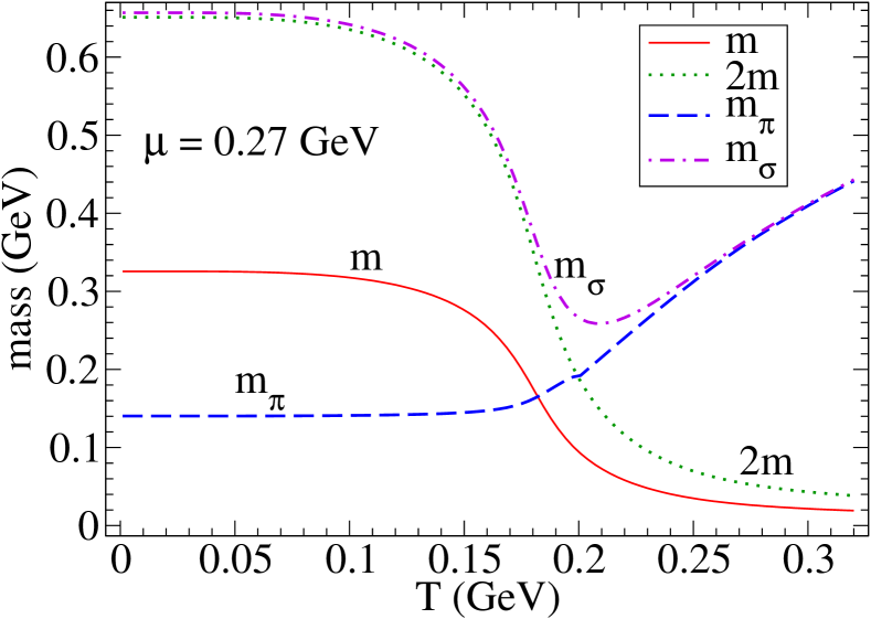
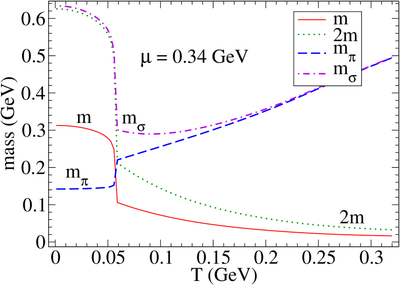
Figure 5: Masses of the $\sigma$ and $\pi$ as functions of the temperature, together with the Hartree quark mass, in the PNJL model at $\mu=0.27$ GeV (top) and $\mu=0.34$ GeV (bottom). The lower figure clearly displays a first order phase transition related to the discontinuity of the chiral condensate occurring at $T^{\chi}_{c}\simeq 0.06$ GeV.

The two panels of Fig. 5 show the behavior of the mesonic masses as functions of temperature, for two different values of the chemical potential. For $\mu=0.27$ GeV the system undergoes a crossover from the low-temperature, chirally broken phase, to the high-temperature, chirally restored one, in analogy to what happens at $\mu=0$. As a consequence, the behaviour of the mesonic masses is very similar to the one shown at vanishing chemical potential (see Fig. 4), the only difference being a lower critical temperature as $\mu$ is increased.

The pattern changes, instead, at $\mu=0.34$ GeV, where a discontinuity in the masses (reflecting an analogous behavior of the chiral condensate $\langle\bar{q}q\rangle$) appears. This can be understood by observing that between $\mu=0.27$ and $0.34$ GeV there exists a critical point Ratti:2006gh , separating a crossover from a first order phase transition.

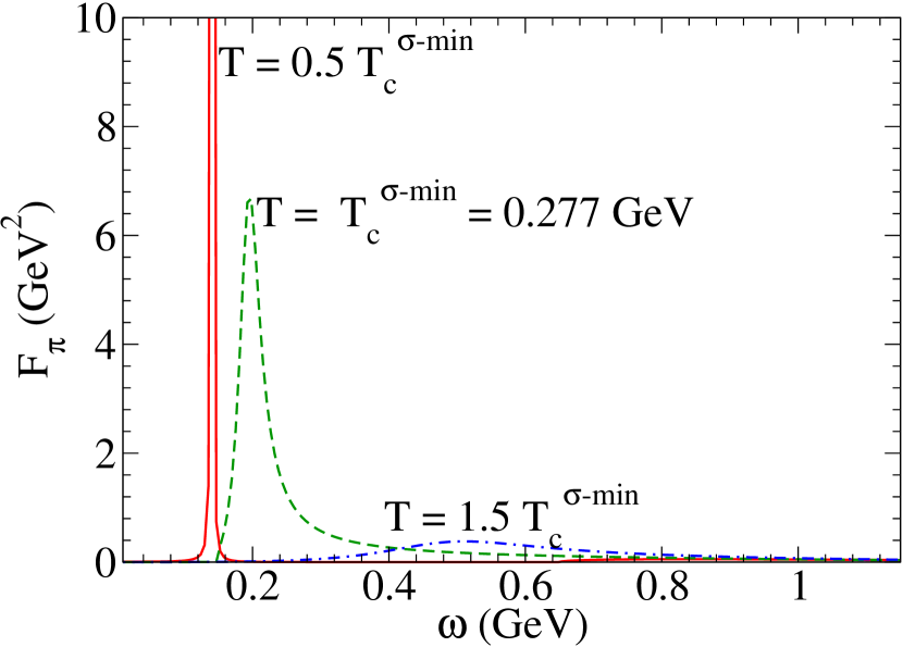
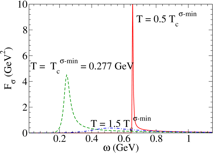
Figure 6: Spectral function $F^{MM}(\omega)$ of the pion (top) and sigma (bottom) in PNJL, at $\vec{q}=\vec{0}$, as a function of $\omega$, for different temperatures and $\mu=0$. The width of the delta peak in the $\pi$ spectral function when $m_{\pi}<2m$ is artificially given by a small, positive $i\eta$.

In concluding this paragraph, we show the pion and $\sigma$ spectral functions in Fig. 6. Notice their progressive broadening as the temperature increases. Besides, they tend to merge for $T>T^{\sigma-min}_{c}$, in the chirally symmetric phase, as expected.

V.3 NJL vs. PNJL: Mesonic masses at $\boldsymbol{\mu=0}$

In Fig. 7 we show a direct comparison between NJL and PNJL results for the mesonic masses at $\mu=0$. According to the features discussed in the previous paragraph, the key quantity which governs the temperature evolution of the mesonic masses is the dressed quark mass. As it is evident from the figure, the main quantitative difference between the results of the two models is the shift of the critical temperature for the phase transition, which turns out to be higher in the PNJL model, with respect to the “classic” NJL one. From a qualitative point of view, there is a good agreement between the results of the two models: in both cases in fact, the $\sigma$ meson mass closely follows the behaviour of $2m$ for small temperatures, decreasing when one approaches the phase transition region. Above $T_{c}$, instead, $m_{\sigma}$ increases with the temperature, merging with the pion mass. This behavior reflects chiral symmetry restoration, a feature which is correctly described by both models, and therefore not spoiled by the coupling of quarks to the Polyakov loop.

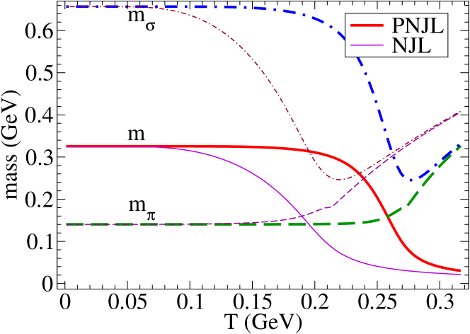
Figure 7: $\sigma$ and $\pi$ masses as functions of the temperature, together with the Hartree quark mass in NJL (thin lines) and PNJL (thick lines) model ($\mu=0$).

V.4 NJL vs. PNJL: the $\boldsymbol{\sigma}$ spectral function

In this paragraph we discuss the width of the $\sigma$ spectral function for the process $\sigma\rightarrow\bar{q}q$, as a function of the reduced temperature $T/T^{\sigma-min}_{c}$. As already anticipated, we find it convenient to rescale $T$ by $T^{\sigma-min}_{c}$ since, interestingly enough, the $\sigma$ spectral function computed in the PNJL model almost coincides with the one evaluated in NJL at $T\simeq T^{\sigma-min}_{c}$. This can be clearly seen in Fig. 8, where the $\sigma$ spectral function at $\vec{q}=\vec{0}$ is plotted vs. frequency. Notice the broadening of the $\sigma$ spectral function in PNJL as compared to the NJL one when $T>T^{\sigma-min}_{c}$, pointing to a stronger production of “free” quarks in this regime.

To quantitatively illustrate these features at zero chemical potential, in the upper panel of Fig. 9 we show the absolute values of the $\sigma$ meson width in the NJL and in the PNJL models, while in the lower panel we show the ratio between the widths evaluated in the two models. The width of the $\sigma$ evaluated in PNJL is smaller than the NJL one below $T^{\sigma-min}_{c}$ and it is larger above $T^{\sigma-min}_{c}$. This is an indication that in PNJL the decay channel $\sigma\rightarrow\bar{q}q$ is reduced at low temperatures with respect to the NJL case. On the contrary, above $T^{\sigma-min}_{c}$ one can interpret the larger width of the quarks bound into the meson as a more efficient deconfinement effect. In spite of the smallness of both absolute widths, the PNJL model entails a reduction up to $\simeq 40$ % for $\Gamma_{\sigma}(PNJL)$, a step toward confinement: this can be seen in the lower panel of Fig. 9, where the relative width $\Gamma_{\sigma}(PNJL)/\Gamma_{\sigma}(NJL)$ is displayed as a function of the reduced temperature.

We also notice that, in both channels and at $\mu=0$, Eq.(72) no longer has a real solution for $T=0.396$ GeV$=2.04T^{\chi}_{c}$ in NJL and $T=0.422$ GeV$=1.65T^{\chi}_{c}$ in PNJL. These can be interpreted as the dissociation temperatures of the model ; the faster (in relative units) occurrence of dissociation in PNJL is in agreement with the larger width of the $\sigma$ meson at high temperatures.

In Fig.9 (bottom) we also report the ratio of widths at a finite chemical potential, $\mu=0.27$ GeV. Here the overall situation is qualitatively similar to what happens at $\mu=0$. However the curve shows some peculiar features, overshooting one at small $T/T_{c}$ (where the absolute widths are both, in any case, very small). This behavior does not lend itself to an immediate physical interpretation since the critical point, in the two models, differs not only for the value of the temperature but also of the chemical potential. Hence the “absolute” value $\mu=0.27$ GeV corresponds to different physical situations: a rescaling for the chemical potential should be performed, but it goes beyond the scope of the present work, since it involves a precise discussion of the phase diagram of the PNJL model compared to the NJL one.

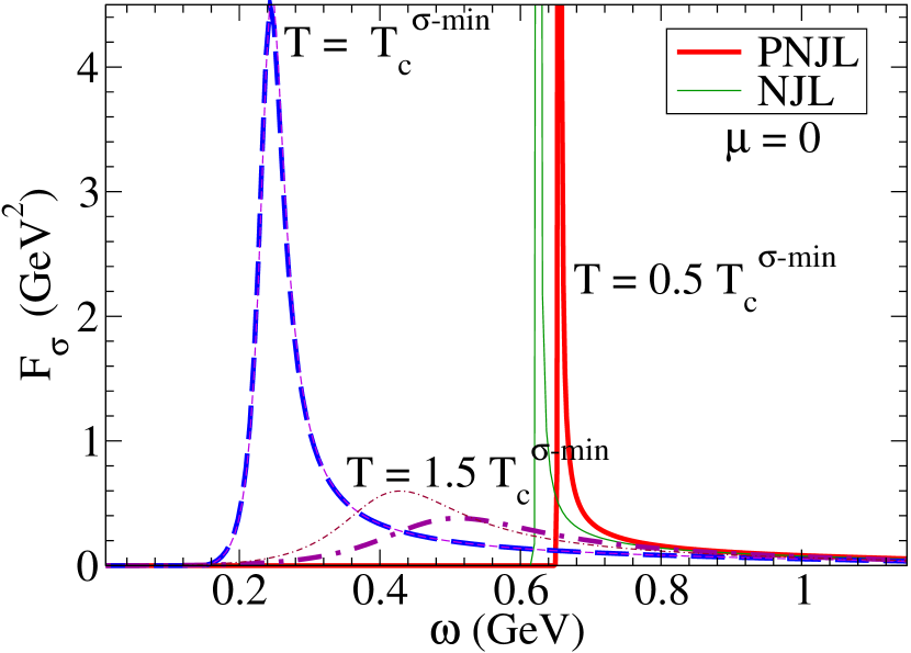
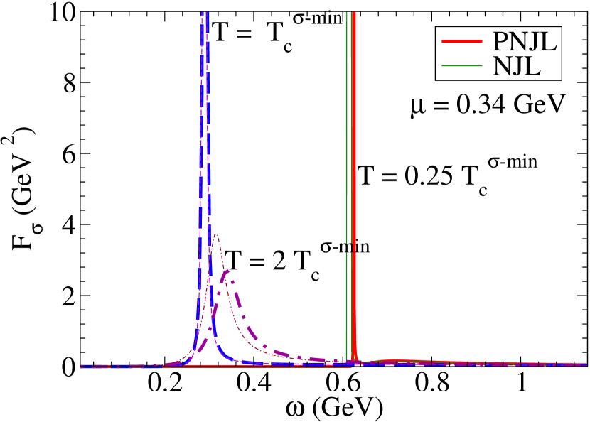
Figure 8: Comparison of the $\sigma$ spectral function at $\vec{q}=\vec{0}$, as a function of $\omega$, for different temperatures and two chemical potentials. Thick lines correspond to PNJL model and thin ones to NJL. Notice the almost perfect coincidence at $T=T^{\sigma-min}_{c}$.

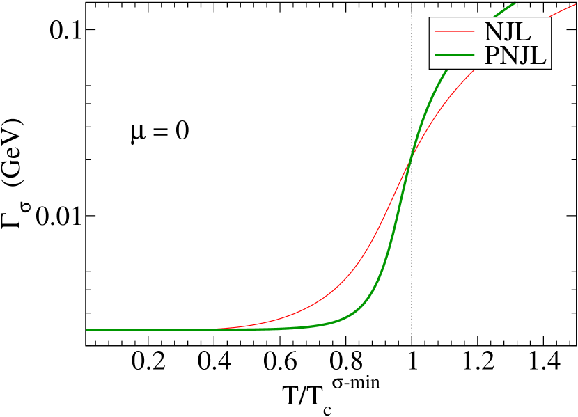
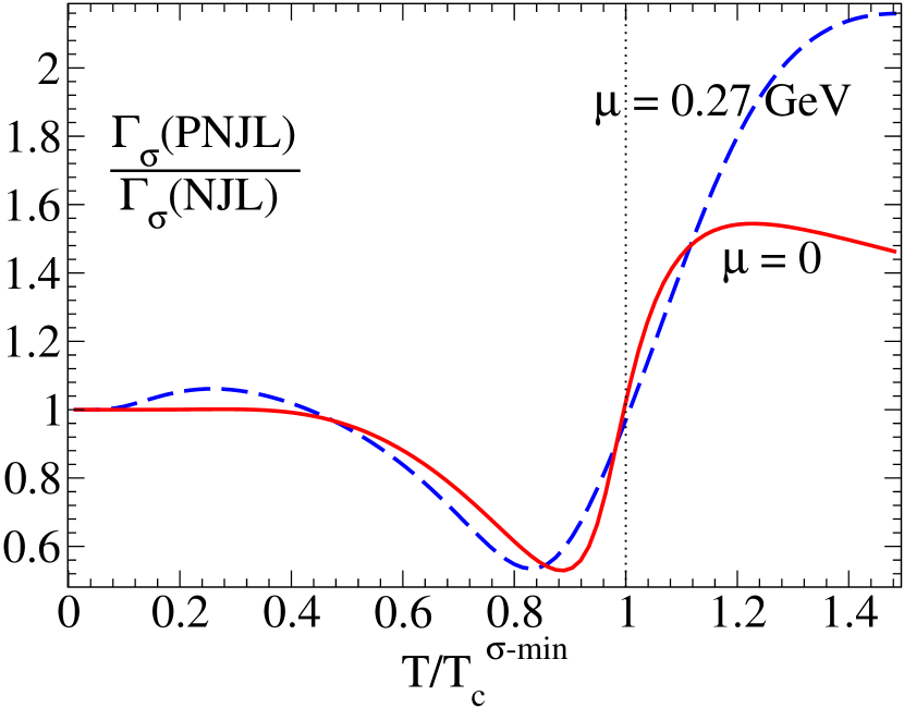
Figure 9: Comparison of the width of the $\sigma$ in NJL and PNJL as a function of the reduced temperature $T/T_{c}$. Top: absolute comparison at zero chemical potential. Bottom: relative width $\Gamma_{\sigma}(PNJL)/\Gamma_{\sigma}(NJL)$ at $\mu=0$ and $\mu=0.27$ GeV. In the latter, a maximum effect below $T_{c}$ ($T\simeq 0.87\,T_{c}$) of $\simeq 40$% can be seen.

VI Conclusions

In the present work, we have investigated the properties of scalar and pseudo-scalar mesons at finite temperature and quark chemical potential in the framework of the Polyakov loop extended Nambu–Jona-Lasinio model. This model has proven to be particularly successful in reproducing two flavour QCD thermodynamics as obtained in lattice calculations Ratti:2005jh : the coupling of quarks to the Polyakov loop produces a statistical suppression of the one- and two-quark contributions to the thermodynamics, thus remarkably improving the NJL model results at low temperatures.

The present work was meant as a test of the PNJL model in the mesonic sector. On the one hand, it was important to check whether the role of pions as Goldstone bosons as well as the pion-$\sigma$ degeneracy in the chirally restored phase are still satisfied after coupling quarks to the Polyakov loop. On the other hand, it was interesting to investigate whether the coupling to the Polyakov loop can cure some problems of the “classic” NJL model description of mesons, such as the unphysical width of the $\sigma$ meson for the process $\sigma\rightarrow\bar{q}q$ in the chirally broken phase.

Finally we also intended to generalize the NJL formalism in order to embody the Polyakov loop coupled to quarks. This turned out to be particularly useful in the mesonic sector. Indeed we have shown the important results that PNJL calculations can be directly deduced from NJL ones (not only for one loop calculations, but to all orders) simply by a redefinition of the usual Fermi – Dirac distribution function.

Our work shows a perfect agreement between the NJL and PNJL results concerning the mesonic masses: in the high temperature phase, pions and $\sigma$ tend to merge, thus displaying the correct pattern for chiral symmetry restoration. In particular, the pions still survive as bound states up to $T_{Mott}\simeq 1.06T^{\chi}_{c}$, and their Goldstone boson nature is still preserved in the chirally broken phase.

As far as the $\sigma$ meson is concerned, no true confinement is observed in the model, since the unphysical width due to the decay into a $\bar{q}q$ pair is still present in the PNJL model. This does not come as a surprise, since no dynamical, self-coupled gluons are embodied in the model Lagrangian. In any case our results in PNJL on the decay width improve slightly the NJL ones.

- (1) M. Mannarelli and R. Rapp, Phys. Rev. C72, 064905 (2005).
- (2) M. Kitazawa, T. Kunihiro and Y. Nemoto, Phys. Lett. B633, 269 (2006).
- (3) S. Datta, F. Karsch, P. Petreczky and I. Wetzorke, Phys. Rev. D69, 094507 (2004).
- (4) E. V. Shuryak and I. Zahed, Phys. Rev. D70, 054507 (2004).
- (5) E. Shuryak, Nucl. Phys. A750, 64 (2005).
- (6) C.Y. Wong, Phys. Rev. C72, 034906 (2005).
- (7) C.Y. Wong, hep-ph/0606200.
- (8) S. Datta, F. Karsch, P. Petreczky and I. Wetzorke, J. Phys. G31, S351 (2005).
- (9) W.M. Alberico, A. Beraudo, A. De Pace and A. Molinari, Phys. Rev. D72, 114011 (2005).
- (10) A. Mocsy and P. Petreczky, Phys. Rev. D73, 074007 (2006).
- (11) V. Koch, A. Majumder and J. Randrup, Phys. Rev. Lett. 95, 182301(2005).
- (12) S. Ejiri, F. Karsch and K. Redlich, Phys. Lett. B633, 275 (2006).
- (13) J.Liao and Edward V. Shuryak, Phys. Rev. D73, 014509 (2006).
- (14) T. Renk and J. Ruppert, hep-ph/0605130.
- (15) J. Ruppert, T. Renk and B. Muller, Phys. Rev. C73, 034907 (2006).
- (16) H. van Hees and R. Rapp, hep-ph/0604269.
- (17) H. van Hees and R. Rapp, hep-ph/0603084.
- (18) G.E. Brown and M. Rho, nucl-th/0509001
- (19) G.E. Brown and M. Rho, nucl-th/0509002
- (20) NA60 Collaboration (R. Arnaldi et al.) Phys. Rev. Lett. 96, 162302 (2006).
- (21) QCD-TARO Collaboration (P. de Forcrand et al.), hep-lat/9901017.
- (22) QCD-TARO Collaboration (I. Pushkina et al.), Phys. Lett. B609 (2005), 265.
- (23) P. Petreczky, J. Phys. G30 (2004), S431.
- (24) S. Wissel et al., hep-lat/0510031.
- (25) T.H. Hansson and I. Zahed, Nucl. Phys. B374 (1992), 277.
- (26) M. Laine and M. Vepsalainen, JHEP 0402 (2004) 004.
- (27) W.M. Alberico, A. Beraudo and A. Molinari, Nucl. Phys. A750 (2005), 359.
- (28) W.M. Alberico, A. Beraudo, P. Czerski and A. Molinari, hep-ph/0605060.
- (29) F. Karsch, M.G. Mustafa, M.H. Thoma, Phys. Lett. B497 (2001), 249.
- (30) P. N. Meisinger and M. C. Ogilvie, Phys. Lett. B 379, 163 (1996).
- (31) P. N. Meisinger, T. R. Miller, and M. C. Ogilvie, Phys. Rev. D 65, 034009 (2002).
- (32) K. Fukushima, Phys. Lett. B 591, 277 (2004).
- (33) A. Mocsy, F. Sannino and K. Tuominen, Phys. Rev. Lett. 92 (2004) 182302
- (34) E. Megias, E. Ruiz Arriola and L. L. Salcedo, Phys. Rev. D 74, 065005 (2006)
- (35) C. Ratti, M. A. Thaler, and W. Weise, Phys. Rev. D73, 014019 (2006).
- (36) C. Ratti, M. A. Thaler and W. Weise, nucl-th/0604025.
- (37) S.K. Ghosh, T.K. Mukherjee, M.G. Mustafa and R. Ray, Phys. Rev. D73, 114007 (2006).
- (38) Y. Nambu and G. Jona-Lasinio, Phys. Rev. 122, 345 (1961).
- (39) T. Hatsuda and T. Kunihiro, Phys. Rev. Lett. 55, 158 (1985).
- (40) V. Bernard, Ulf-G. Meissner and I. Zahed, Phys. Rev. Lett. 59 (1987) 966.
- (41) V. Bernard, Ulf-G. Meissner and I. Zahed, Phys. Rev. D 36 (1987) 819.
- (42) M. Jaminon, G. Ripka and P. Stassart, Nucl. Phys. A 504 (1989) 733.
- (43) U. Vogl and W. Weise, Prog. Part. Nucl. Phys. 27, 195 (1991).
- (44) S. P. Klevansky, Rev. Mod. Phys. 64, 649 (1992).
- (45) M. Lutz, S. Klimt and W. Weise, Nucl. Phys. A 542 (1992) 521.
- (46) T. Hatsuda and T. Kunihiro, Phys. Rep. 247, 221 (1994).
- (47) V. Bernard, Ulf-G. Meissner, A. Blin and B. Hiller, Phys. Lett. B 253 (1991) 443.
- (48) G. Ripka, Quarks Bound by Chiral Fields, Clarendon, Oxford (1997).
- (49) M. Buballa, Phys. Rept. 407, 205 (2005).
- (50) R.D. Pisarski Phys. Rev. D62, 111501 (2000).
- (51) R.D. Pisarski, Published in *Cargese 2001, QCD perspectives on hot and dense matter*, 353-384, hep-ph/0203271.
- (52) A.M. Polyakov, Phys. Lett. B72, 477 (1978).
- (53) G. ’t Hooft, Nucl. Phys. B138, 1 (1978).
- (54) B. Svetitsky and L.G. Yaffe, Nucl. Phys. B210, 423 (1982).
- (55) L.D. McLerran and B. Svetitsky, Phys. Rev. D24, 450 (1981).
- (56) H.J. Rothe, Lattice Gauge Theory: An introduction, World Scientific (2005).
- (57) O. Kaczmarek, F. Karsch, P. Petreczky, and F. Zantow, Phys. Lett. B 543, 41 (2002).
- (58) G. Boyd et al., Nucl. Phys. B469 (1996), 419.
- (59) S. Roessner, C. Ratti and W. Weise, arXiv:hep-ph/0609281.
- (60) P. N. Meisinger, M. C. Ogilvie and T. R. Miller, Phys. Lett. B 585, 149 (2004)
- (61) T. M. Schwarz, S. P. Klevansky, and G. Papp, Phys. Rev. C60, 055205 (1999).
- (62) M. Oertel, M. Buballa, and J. Wambach, Phys. Atom. Nucl. 64, 698 (2001).
- (63) S. P. Klevansky and R. H. Lemmer, arXiv:hep-ph/9707206.
- (64) H. J. Schulze, J. Phys. G20, 531 (1994).
- (65) R. M. Davidson and E. Ruiz Arriola, Phys. Lett. B359, 273 (1995).
- (66) T. Hatsuda and T. Kunihiro, Phys. Lett. B185, 304 (1987).
- (67) W. Florkowski and B. L. Friman, Acta Phys. Polon. B25, 49 (1994).
- (68) R.-K. Su and G.-T. Zheng, J. Phys. G16, 203 (1990).
- (69) R. L. S. Farias, G. Krein, and O. A. Battistel, AIP Conf. Proc. 739, 431 (2005).
- (70) M. Oertel, arXiv:hep-ph/0012224.
- (71) P. Costa, M. C. Ruivo, C. A. de Sousa and Y. L. Kalinovsky, Phys. Rev. C70, 025204 (2004).
- (72) P. Costa, M. C. Ruivo, and Y. L. Kalinovsky, Phys. Lett. B560, 171 (2003).
- (73) A. E. Dorokhov et al., Z. Phys. C75, 127 (1997).