QCD Coulomb gauge approach to hybrid mesons

Abstract

An effective Coulomb gauge Hamiltonian, $H_{\rm eff}$, is used to calculate the light ($u\bar{u}g$), strange ($s\bar{s}g$) and charmed ($c\bar{c}g$) hybrid meson spectra. For the same two parameter $H_{\rm eff}$ providing glueball masses consistent with lattice results and a good description of the observed $u,d,s$ and $c$ quark mesons, a large-scale variational treatment predicts the lightest hybrid has $J^{PC}=0^{++}$ and mass 2100 MeV. The lightest exotic $1^{-+}$ state is just above 2200 MeV, near the upper limit of lattice and Flux Tube predictions. These theoretical formulations all indicate the observed $1^{-+}$ $\pi_{1}(1600)$ and, more clearly, $\pi_{1}(1400)$ are not hybrid states. The Coulomb gauge approach further predicts that in the strange and charmed sectors, respectively, the ground state hybrids have $1^{+-}$ with masses 2125 and 3830 MeV, while the first exotic $1^{-+}$ states are at 2395 and 4020 MeV. Finally, using our hybrid wavefunctions, dimensional counting rules and the Franck-Condon principle, novel experimental signatures are presented to assist light and heavy hybrid meson searches.

I Introduction

Following the “Eightfold Way” (Gell-Mann and Ne’eman), the “Quark Model” (Gell-Mann and Zweig), along with subsequent extensions, has generally explained the observed hadronic spectrum. This is especially true for heavy flavored mesons where it is now clear that higher order QCD corrections can be ignored or treated perturbatively. Even in the light sector, the phenomenological quark model works reasonably well. However, the existence of hadrons with exotic quantum numbers (i.e. $J^{PC}$ states not possible in $q\bar{q}$ or $qqq$ systems) clearly reveals this model is not complete. Related, it is expected that there are exotic hadrons with conventional quantum numbers that also can not be described by the quark model, e.g., glueballs $gg$, hybrid mesons $q\overline{q}g$ and tetraquarks $q\overline{q}q\overline{q}$.

Possible experimental evidence for a $1^{-+}$ exotic state was first reported in 1988 Alde , but the situation was not clarified until several years later. Now it is believed that there exist two states with these quantum numbers below 2 GeV: $\pi_{1}(1400)$ E852-1 ; E852-2 and $\pi_{1}(1600)$ E852-3 ; E852-4 (note, a recent analysis ds finds no evidence for either candidate). There are also other reported hybrid candidates with $J^{PC}=$ $0^{-+}$ Amelin ; Zaitsev , $1^{--}$ Donnachie and $2^{-+}$ Karch ; Adomeit ; Barberis .

Theoretically, the structure of the $\pi_{1}$ states remains unclear. They could be hybrid or tetraquark mesons with most theoretical studies Kalashnikova:2001ke ; Buisseret:2006sz investigating the former. Lattice gauge simulations Bernard1 ; Bernard2 ; Lacock ; Hedditch ; Luo predict the lightest hybrid meson is between 1.7 and 2.1 GeV and results from the Flux Tube model Barnes ; Close ; Katja also span much of this range. Only vintage Bag model Bag calculations yield a lower mass, between 1.3 and 1.8 GeV, but Ref.  Iddir argues that the $\pi_{1}(1400)$ is not a hybrid. Table 1 list predictions for the $u/d$, $s$ and $c$ $1^{-+}$ hybrid mesons.

Model [Reference]	$u/d$ hybrid	$s$ hybrid	$c$ hybrid
Lattice QCD [15-19, 25-27]	1.7 - 2.1	1.9	4.2 - 4.4
Flux Tube Barnes ; Close ; Katja	1.8 - 2.1	2.1 - 2.3	4.1 - 4.5
Bag Model Bag	1.3 - 1.8		3.9

Table 1: Published predicted $1^{-+}$ masses, in GeV, for light, strange and charmed hybrid mesons.

In this work, we study $q\bar{q}g$ hybrid states using a field theoretical, relativistic many-body approach based upon an effective QCD Hamiltonian, $H_{\rm eff}$, formulated in the Coulomb gauge. This model successfully describes the meson spectrum LC2 ; LCSS and is also consistent LBC with lattice glueball (and oddball) predictions. Using standard bare current quark masses, it properly incorporates chiral symmetry, yet dynamically generates a constituent mass and spontaneous chiral symmetry breaking LC1 . Further, it provides a good description of the vacuum properties (quark and gluon condensates), and respects the global, internal symmetries of QCD, as well as the spatial Euclidean group, all within a minimal two parameter theory. Our work also extends an earlier hybrid calculation LChybrid by including previously omitted terms in the Hamiltonian and by comprehensively predicting the light, strange and charmed hybrid meson spectra.

This paper is organized into 8 sections. In Sections II and III the effective Hamiltonian is presented along with an improved hyperfine interaction which provides realistic spin splittings in both light and heavy mesons LCSS and, for the first time, the rigorous non-abelian contributions from the color magnetic fields. Section IV details the corresponding improved quark and gluon gap equations and a variational formulation for the hybrid meson problem is developed in Sec. V. Calculations and new results are discussed in Sec. VI, while in Sec. VII we develop novel experimental signatures for observing hybrid mesons having both conventional and exotic quantum numbers. Finally, we summarize results and conclusions in Sec. VIII.

II Effective Hamiltonian

Our effective, quark-gluon Hamiltonian is an approximation to the exact Coulomb gauge QCD Hamiltonian T-D-Lee and is given by (summation over repeated indices is used throughout this paper)

$$H_{\rm eff} = H_{q}+H_{g}+H_{qg}+H_{C}$$ (1)

$$H_{q} = \int d{\boldsymbol{x}}\Psi^{\dagger}({\boldsymbol{x}})[-i{\mbox{\boldmath$\alpha$\unboldmath}}\cdot{\mbox{\boldmath$\nabla$\unboldmath}}+\beta m]\Psi({\boldsymbol{x}})$$ (2)

$$H_{g} = \frac{1}{2}\int d{\boldsymbol{x}}\left[{\bf\Pi}^{a}({\boldsymbol{x}})\cdot{\bf\Pi}^{a}({\boldsymbol{x}})+{\bf B}^{a}({\boldsymbol{x}})\cdot{\bf B}^{a}({\boldsymbol{x}})\right]$$ (3)

$$H_{qg} = g\int d{\boldsymbol{x}}\;{\bf J}^{a}({\boldsymbol{x}})\cdot{\bf A}^{a}({\boldsymbol{x}})$$ (4)

$$H_{C} = -\frac{1}{2}\int d{\boldsymbol{x}}d{\boldsymbol{y}}\rho^{a}({\boldsymbol{x}})\hat{V}(\arrowvert{\boldsymbol{x}}-{\boldsymbol{y}}\arrowvert)\rho^{a}({\boldsymbol{y}})\ .$$ (5)

Here $g$ is the QCD coupling, $\Psi$ is the quark field with current quark mass $m$, ${\bf A}^{a}$ are the gluon fields satisfying the transverse gauge condition, $\nabla$ $\cdot$ ${\bf A}^{a}=0$, $a=1,2,...8$, ${\bf\Pi}^{a}$ are the conjugate fields and ${\bf B}^{a}$ are the non-abelian magnetic fields

$${\bf B}^{a}=\nabla\times{\bf A}^{a}+\frac{1}{2}gf^{abc}{\bf A}^{b}\times{\bf A}^{c}\ .$$ (6)

The color densities, $\rho^{a}({\boldsymbol{x}})$, and quark color currents, ${\bf J}^{a}$, are related to the fields by

$$\rho^{a}({\boldsymbol{x}}) = \Psi^{\dagger}({\boldsymbol{x}})T^{a}\Psi({\boldsymbol{x}})+f^{abc}{\bf A}^{b}({\boldsymbol{x}})\cdot{\bf\Pi}^{c}({\boldsymbol{x}})$$ (7)

$${\bf J}^{a} = \Psi^{\dagger}({\boldsymbol{x}})\mbox{\boldmath$\alpha$\unboldmath}T^{a}\Psi({\boldsymbol{x}})\ ,$$ (8)

where $T^{a}=\frac{\lambda^{a}}{2}$ and $f^{abc}$ are the $SU_{3}$ color matrices and structure constants, respectively.

The bare parton fields have the following normal mode expansions (bare quark spinors $u,v$, helicity, $\lambda=\pm 1$, and color vectors $\hat{\boldsymbol{\epsilon}}_{{\cal C}=1,2,3}$)

$$\Psi(\boldsymbol{x}) = \int\!\!\frac{d\boldsymbol{k}}{(2\pi)^{3}}\Psi_{{\cal C}}(\boldsymbol{k})e^{i\boldsymbol{k}\cdot\boldsymbol{x}}\hat{\boldsymbol{\epsilon}}_{\cal C}$$ (9)

$$\Psi_{{\cal C}}(\boldsymbol{k}) = {u}_{\lambda}(\boldsymbol{k})b_{\lambda{\cal C}}(\boldsymbol{k)}+{v}_{\lambda}(-\boldsymbol{k})d^{\dagger}_{\lambda{\cal C}}(\boldsymbol{-k)}$$ (10)

$${\bf A}^{a}({\boldsymbol{x}}) = \int\frac{d{\boldsymbol{k}}}{(2\pi)^{3}}\frac{1}{\sqrt{2k}}[{\bf a}^{a}({\boldsymbol{k}})+{\bf a}^{a{\dagger}}(-{\boldsymbol{k}})]e^{i{\boldsymbol{k}}\cdot{\boldsymbol{x}}}\ \ \$$ (11)

$${\bf\Pi}^{a}({\boldsymbol{x}}) = -i\int\!\!\frac{d{\boldsymbol{k}}}{(2\pi)^{3}}\sqrt{\frac{k}{2}}[{\bf a}^{a}({\boldsymbol{k}})-{\bf a}^{a{\dagger}}(-{\boldsymbol{k}})]e^{i{\boldsymbol{k}}\cdot{\boldsymbol{x}}}\!,$$ (12)

with the Coulomb gauge transverse condition, ${\boldsymbol{k}}\cdot{\bf a}^{a}({\boldsymbol{k}})=\\ (-1)^{\mu}k_{\mu}a_{-\mu}^{a}({\boldsymbol{k}})=0$. Here $b_{\lambda{\cal C}}(\boldsymbol{k)}$, $d_{\lambda{\cal C}}(\boldsymbol{-k)}$ and $a_{\mu}^{a}({\boldsymbol{k}})$ ($\mu=0,\pm 1$) are the bare quark, anti-quark and gluon Fock operators, the latter satisfying the transverse commutation relations,

$$[a^{a}_{\mu}({\boldsymbol{k}}),a^{b\dagger}_{\mu^{\prime}}({\boldsymbol{k}}^{\prime})]=(2\pi)^{3}\delta_{ab}\delta^{3}({\boldsymbol{k}}-{\boldsymbol{k}}^{\prime})D_{{\mu}{\mu^{\prime}}}({\boldsymbol{k}})\ ,$$ (13)

with

$$D_{{\mu}{\mu^{\prime}}}({\boldsymbol{k}})=\delta_{{\mu}{\mu^{\prime}}}-(-1)^{\mu}\frac{k_{\mu}k_{-\mu^{\prime}}}{k^{2}}\ .$$ (14)

Confinement is described by a Cornell type potential,

$$\hat{V}(r=|{\boldsymbol{x}}-{\boldsymbol{y}}|) = {\hat{V}}_{C}(r)+{\hat{V}}_{L}(r)$$ (15)

$$\hat{V}_{C}(r) = -\frac{\alpha_{s}}{r}$$ (16)

$$\hat{V}_{L}(r) = \sigma r,$$ (17)

where the string tension, $\sigma=0.135$ GeV², and $\alpha_{s}=\frac{g^{2}}{4\pi}=0.4$ have been previously determined. The Fourier transform of $\hat{V}$ is denoted by $V$ and in momentum space these potentials take the form $V_{L}(|\boldsymbol{p}|)=-8\pi\sigma/p^{4}$, $V_{C}(|\boldsymbol{p}|)=-4\pi\alpha_{s}/p^{2}$. For comparison and also to provide hadronic structure sensitivity to potential form, we report predictions using a confining potential SS having a renormalization improved short-ranged behavior. This potential was utilized in a previous meson study LCSS and has the momentum space representation

$${V}(|\boldsymbol{p}|)=\left\{\begin{array}[]{ll}-\frac{8.04}{p^{2}}\frac{\ln^{-0.62}(\frac{p^{2}}{m_{g}^{2}}+0.82)}{\ln^{0.8}(\frac{p^{2}}{m_{g}^{2}}+1.41)}&\textrm{ $p>m_{g}$}\\ -\frac{12.25m^{1.93}_{g}}{p^{3.93}}&\textrm{$p<m_{g}$}\end{array}\right.\ .$$ (18)

The parameter $m_{g}$ sets the string tension and is related to $\sigma$ by $m_{g}\cong\sqrt{8\pi\sigma/12.25}\approx 600$ MeV.

III Hamiltonian $g^{2}$ Corrections

As mentioned above, a previous hybrid application LChybrid used this Hamiltonian but set the QCD coupling, $g$, to zero. This truncation eliminated the quark-gluon interaction, ${\bf J}^{a}\cdot{\bf A}^{a}$, or “hyperfine” term, Eq. (4), and also the non-linear (non-abelian) component of the color magnetic fields, Eqs. (3, 6). Now, both are included so that the non-confining part of the Hamiltonian is consistent to order $g^{2}$.

III.1 Hyperfine correction

Following LCSS , the Hamiltonian term $H_{qg}$ containing the ${\bf J}^{a}\cdot{\bf A}^{a}$ operators is included using perturbation theory to second order in $g$. Then, integrating over the gluonic degrees of freedom yields an effective quark hyperfine interaction with a ${\bf J}^{a}\cdot{\bf J}^{a}$ form. This contribution is represented by the Feynman diagrams in Fig. 1.

The resulting transverse hyperfine interaction is

$$V_{T}=\frac{1}{2}\int\!\!\!\int\!\!d\boldsymbol{x}d\boldsymbol{y}J_{i}^{a}(\boldsymbol{x})\hat{U}_{ij}(\boldsymbol{x,y})J_{j}^{a}(\boldsymbol{y}),$$ (19)

where the kernel reflects the transverse gauge

$$\hat{U}_{ij}(\boldsymbol{x,y})=\bigg{(}\delta_{ij}-\frac{\nabla_{i}\nabla_{j}}{\nabla^{2}}\bigg{)}_{\boldsymbol{x}}\hat{U}(|\boldsymbol{x-y}|).$$ (20)

For $\hat{U}$ we choose a modified Yukawa potential which incorporates a dynamical mass, $m_{g}=600$ MeV, for the exchanged gluon as explained in LCSS . Fourier transforming to momentum space, this continuous potential takes the form

$${U}(p)=\left\{\begin{array}[]{ll}-\frac{8.04}{p^{2}}\frac{\ln^{-0.62}(\frac{p^{2}}{m_{g}^{2}}+0.82)}{\ln^{0.8}(\frac{p^{2}}{m_{g}^{2}}+1.41)}&\textrm{ $p>m_{g}$}\\ -\frac{24.50}{p^{2}+m_{g}^{2}}&\textrm{$p<m_{g}$}\end{array}\right.\ .$$ (21)

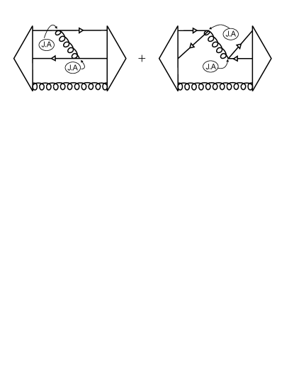
Figure 1: The hyperfine correction entails the exchange of a gluon between $q$ and $\overline{q}$ and $q\overline{q}$ annihilation.

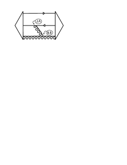
Figure 2: The non-abelian correction with triple gluon vertices.

III.2 Non-abelian correction

Similarly, the non-abelian components of the color magnetic fields, $gf^{abc}{\bf A}^{b}\times{\bf A}^{c}$, in the kinetic energy are also included perturbatively through $({\bf J}^{a}\cdot{\bf A}^{a})({\bf B}^{a}\cdot{\bf B}^{a})$. The resulting non-abelian interaction is represented by the Feynman diagram in Fig. 2 and is given by

$$V_{NA}=\frac{1}{4}\int\!\!\!\int\!\!d\boldsymbol{x}d\boldsymbol{y}f^{abc}\varepsilon_{ijk}\varepsilon_{ilm}[J^{a}_{h}(\boldsymbol{y})(\nabla_{j}^{(\boldsymbol{x})}\hat{U}_{kh}(\boldsymbol{x,y}))A^{b}_{l}(\boldsymbol{x})A^{c}_{m}(\boldsymbol{x})+$$ (22)

$$J^{b}_{h}(\boldsymbol{y})(\nabla_{j}^{(\boldsymbol{x})}A^{a}_{k}(\boldsymbol{x}))\hat{U}_{lh}(\boldsymbol{x,y})A^{c}_{m}(\boldsymbol{x})+J^{c}_{h}(\boldsymbol{y})(\nabla_{j}^{(\boldsymbol{x})}A^{a}_{k}(\boldsymbol{x}))A^{b}_{l}(\boldsymbol{x})\hat{U}_{mh}(\boldsymbol{x,y})].$$

where $\hat{U}_{ij}$ is the same kernel appearing in the hyperfine potential.

IV Gap Equation

Having defined the model Hamiltonian, the next step is to calculate the ground state. Since we are free to expand the field operators in any complete basis, we follow the Bardeen-Cooper-Schriffer (BCS) method and perform a Bogoliubov-Valatin rotation,

$$B_{\lambda{\cal C}}(\boldsymbol{k)} = \cos\frac{\theta_{k}}{2}b_{\lambda{\cal C}}(\boldsymbol{k)}-\lambda\sin\frac{\theta_{k}}{2}d^{\dagger}_{\lambda{\cal C}}(\boldsymbol{-k)}$$

$$D_{\lambda{\cal C}}(\boldsymbol{-k)} = \cos\frac{\theta_{k}}{2}d_{\lambda{\cal C}}(\boldsymbol{-k)}+\lambda\sin\frac{\theta_{k}}{2}b^{\dagger}_{\lambda{\cal C}}(\boldsymbol{k)}$$

$${\boldsymbol{\alpha}}^{a}(\boldsymbol{k}) = \cosh\Theta_{k}{\bf a}^{a}(\boldsymbol{k})+\sinh\Theta_{k}{{\bf a}^{a}}^{\dagger}(-\boldsymbol{k})\ ,$$ (23)

which transforms the bare particle operators ${\bf a}^{a}$, $b_{\lambda{\cal C}}$ and $d_{\lambda{\cal C}}$ into the dressed, quasi-particle operators ${\boldsymbol{\alpha}}^{a}$, $B_{\lambda{\cal C}}$ and $D_{\lambda{\cal C}}$, respectively. Now the fields are

$$\Psi_{{\cal C}}(\boldsymbol{k}) = {\cal U}_{\lambda}(\boldsymbol{k})B_{\lambda{\cal C}}(\boldsymbol{k)}+{\cal V}_{\lambda}(-\boldsymbol{k})D^{\dagger}_{\lambda{\cal C}}(\boldsymbol{-k)}$$

$${\bf A}^{a}({\boldsymbol{x}}) = \int\frac{d{\boldsymbol{k}}}{(2\pi)^{3}}\frac{1}{\sqrt{2\omega_{k}}}[{\boldsymbol{\alpha}}^{a}({\boldsymbol{k}})+{\boldsymbol{\alpha}}^{a{\dagger}}(-{\boldsymbol{k}})]e^{i{\boldsymbol{k}}\cdot{\boldsymbol{x}}}$$

$${\bf\Pi}^{a}({\boldsymbol{x}}) = -i\int\!\!\frac{d{\boldsymbol{k}}}{(2\pi)^{3}}\sqrt{\frac{\omega_{k}}{2}}[{\boldsymbol{\alpha}}^{a}({\boldsymbol{k}})-{\boldsymbol{\alpha}}^{a{\dagger}}(-{\boldsymbol{k}})]e^{i{\boldsymbol{k}}\cdot{\boldsymbol{x}}}\ ,$$

where $\omega_{k}=ke^{-2\Theta_{k}}$. Note that the dressed quark expansion remains functionally invariant with respect to the bare case since the quasi-particle spinors have the inverse rotation

$${\cal U}_{\lambda}(\boldsymbol{k}) = \cos\frac{\theta_{k}}{2}u_{\lambda}(\boldsymbol{k})-\lambda\sin\frac{\theta_{k}}{2}v_{\lambda}(-\boldsymbol{k})$$ (26)

$$= \frac{1}{\sqrt{2}}\left[\begin{array}[]{c}\sqrt{1+\sin\phi_{k}}\;\;\chi_{\lambda}\\ \sqrt{1-\sin\phi_{k}}\;\boldsymbol{\sigma}\cdot{\bf\hat{\boldsymbol{k}}}\;\;\chi_{\lambda}\\ \end{array}\right]$$

$${\cal V}_{\lambda}(-\boldsymbol{k}) = \cos\frac{\theta_{k}}{2}v_{\lambda}(-\boldsymbol{k})+\lambda\sin\frac{\theta_{k}}{2}u_{\lambda}(\boldsymbol{k})$$ (29)

$$= \frac{1}{\sqrt{2}}\left[\begin{array}[]{c}-\sqrt{1-\sin\phi_{k}}\;\boldsymbol{\sigma}\cdot{\bf\hat{\boldsymbol{k}}}\;\;\chi_{\lambda}\\ \sqrt{1+\sin\phi_{k}}\;\;\chi_{\lambda}\\ \end{array}\right].$$

Here the quark gap angle, $\phi_{k}=\phi(k)$, is related to the BCS angle $\theta_{k}$ by $tan(\phi_{k}-\theta_{k})=m/k$. The quasi-particle (BCS) vacuum, defined by $B_{\lambda{\cal C}}|\Omega\rangle=D_{\lambda{\cal C}}|\Omega\rangle=\alpha^{a}_{\mu}|\Omega\rangle=0$, is connected to the bare parton one, $b_{\lambda{\cal C}}|0\rangle=d_{\lambda{\cal C}}|0\rangle=a^{a}_{\mu}|0\rangle=0$, by

$$|\Omega_{quark}\rangle=e^{-\int\!\!\frac{d\boldsymbol{k}}{(2\pi)^{3}}\lambda\tan\frac{\theta_{k}}{2}b^{\dagger}_{\lambda{\cal C}}(\boldsymbol{k})d^{\dagger}_{\lambda{\cal C}}(-\boldsymbol{k})}|0\rangle$$

$$|\Omega_{gluon}\rangle=e^{-\!\!\int\!\!\frac{d\boldsymbol{k}}{(2\pi)^{3}}\frac{1}{2}\tanh\Theta_{k}D_{\mu\mu^{\prime}}({\boldsymbol{k}})a_{\mu}^{a{\dagger}}(\boldsymbol{k})a_{\mu^{\prime}}^{a{\dagger}}(-\boldsymbol{k})}|0\rangle\ .$$

The BCS vacuum, $|\Omega\rangle=|\Omega_{quark}\rangle\otimes|\Omega_{gluon}\rangle$, now contains quark and gluon condensates (correlated $q\bar{q}$ and $gg$ Cooper pairs). Performing a variational minimization of the vacuum expectation value of the Hamiltonian, $\delta\langle\Omega|H_{\rm eff}|\Omega\rangle=0$, independently with respect to $\phi_{k}$ and $\omega_{k}$, yields the mass gap equations for each sector

$$ks_{k}-mc_{k}= \frac{2}{3}\int\!\!\frac{d\boldsymbol{q}}{(2\pi)^{3}}\left[(s_{k}c_{q}x-s_{q}c_{k})V(|\boldsymbol{k-q}|)\right.$$

$$- \left.2c_{k}s_{q}{U}(\arrowvert{\boldsymbol{k}}-{\boldsymbol{q}}\arrowvert)+2c_{q}s_{k}{W}(\arrowvert{\boldsymbol{k}}-{\boldsymbol{q}}\arrowvert)\right]$$ (30)

$$\omega_{k}^{2} = k^{2}-\frac{3}{4}\int\!\!\frac{d\boldsymbol{q}}{(2\pi)^{3}}V(|\boldsymbol{k-q}|)[1+x^{2}]\bigg{(}\frac{\omega_{q}^{2}-\omega_{k}^{2}}{\omega_{q}}\bigg{)}$$ (31)

$$+ \frac{3}{4}\;g^{2}\int\!\!\frac{d\boldsymbol{q}}{(2\pi)^{3}}\frac{1-x^{2}}{\omega_{q}}\ ,$$

where

$${W}({|\boldsymbol{k}}-{\boldsymbol{q}}|)\equiv{U}(|{\boldsymbol{k}}-{\boldsymbol{q}}|)\frac{x(k^{2}+q^{2})-qk(1+x^{2})}{\arrowvert{\boldsymbol{k}}-{\boldsymbol{q}}\arrowvert^{2}}\ ,$$ (32)

with $s_{k}=sin\phi_{k}$, $c_{k}=cos\phi_{k}$ and $x={\boldsymbol{k}}\cdot{\boldsymbol{q}}$. The last term in Eq. (31) originates from the non-abelian component of the gluon kinetic energy. Dimensional analysis of the above integrals reveals that the first equation is UV finite for the linear potential since $V_{L}(|\boldsymbol{p}|)=-8\pi\sigma/p^{4}$, but not for the Coulomb potential $V_{C}(|\boldsymbol{p}|)=-4\pi\alpha_{s}/p^{2}$. In Eq. (31) there are both logarithmical and quadratical divergences in the UV region and an integration cutoff, $\Lambda=4$ GeV, determined in previous studies is used.

Once the current quark masses are fixed, the gap equations can be solved numerically for the quark and gluon gap angles. Using $|q\rangle=B_{\lambda{\cal C}}(\boldsymbol{k})^{\dagger}|\Omega\rangle$ and $|g\rangle=\alpha^{a}_{\mu}(\boldsymbol{k})^{\dagger}|\Omega\rangle$, the quark and gluon self-energies are respectively

$$\epsilon_{k} \equiv \langle q|H_{\rm eff}|q\rangle=ms_{k}+kc_{k}-$$

$$\frac{2}{3} \int \!\!\frac{d\boldsymbol{q}}{(2\pi)^{3}}\left[[s_{k}s_{q}+c_{q}c_{k}x]V(|\boldsymbol{k-q}|)\right.$$ (33)

$$+ \left.\!\!\!\!2s_{k}s_{q}{U}(\arrowvert{\boldsymbol{k}}-{\boldsymbol{q}}\arrowvert)+2c_{q}c_{k}{W}(\arrowvert{\boldsymbol{k}}-{\boldsymbol{q}}\arrowvert)\right]$$

and, for fixed color index $a$ (no sum),

$$\varepsilon^{\mu\mu^{\prime}}_{k} \equiv \langle\Omega|\alpha^{a}_{\mu}({\boldsymbol{k}})\,H_{\rm eff}\,\alpha^{a}_{\mu^{\prime}}({\boldsymbol{k}})^{\dagger}|\Omega\rangle=\frac{\omega^{2}_{k}+k^{2}}{2\omega_{k}}\delta_{\mu\mu^{\prime}}$$ (34)

$$- \frac{3}{4}\int\frac{d{\boldsymbol{q}}}{(2\pi)^{3}}V(|{\boldsymbol{k}}-{\boldsymbol{q}}|)\frac{\omega_{k}^{2}+\omega_{q}^{2}}{\omega_{q}\omega_{k}}D_{\mu\mu^{\prime}}({\boldsymbol{q}})$$

$$+ \frac{9}{2}g^{2}\int\frac{d{\boldsymbol{q}}}{(2\pi)^{3}}\frac{1}{2\omega_{k}\omega_{q}}\times$$

$$\left[2D_{\mu\mu^{\prime}}({\boldsymbol{k}})-D_{\mu\nu}({\boldsymbol{k}})D_{\nu\nu^{\prime}}({\boldsymbol{q}})D_{\nu^{\prime}\mu^{\prime}}({\boldsymbol{k}})\right]\ ,$$

both of which are infrared divergent in the presence of an infrared enhanced kernel. This is a welcomed feature of this approach, as colored states are removed from the spectrum. The infrared divergence cancels however in bound state equations for color singlet states leading to a physical spectrum of mesons and baryons.

V Hybrid Mesons

In previous publications LC1 ; LC2 ; LCSS ; LBC we have used this model to study the two-body meson and glueball systems by diagonalizing $H_{\rm eff}$ using the Tamm-Dancoff and Random Phase approximations. We also made predictions for three-body glueballs (oddballs) LBC and published LChybrid a brief study of the three-body hybrid meson using a variational treatment. We now extend the latter and also provide more complete details of the variational calculation.

V.1 Wavefunction ansatz and quantum numbers

Following our initial study LChybrid , we work in the hybrid center of momentum system and denote the momenta of the dressed quark, anti-quark and gluon by ${\boldsymbol{q}}$, ${\bar{\boldsymbol{q}}}$ and ${\boldsymbol{g}}$, respectively. We then define ${{\boldsymbol{q}}_{+}\equiv\frac{{\boldsymbol{q}}+\overline{\boldsymbol{q}}}{2}}$, ${\boldsymbol{q}_{-}\equiv q-\overline{q}}$ and note that ${\boldsymbol{g}=-\boldsymbol{q}-\overline{q}}=-2{\boldsymbol{q}}_{+}$.

The color structure of a $q\bar{q}g$ hybrid is determined by SU(3) algebra

$$(3\otimes\overline{3})\otimes 8 = (8\oplus 1)\otimes 8=(8\otimes 8)\oplus(8\otimes 1)$$ (35)

$$= 27\oplus 10\oplus 10\oplus 8\oplus 8\oplus 1\oplus 8.$$

Note for an overall color singlet the quarks must be in an octet state like the gluon. As discussed below, this leads to a repulsive $q\bar{q}$ interaction, confirmed by lattice at short range, which raises the mass of the hybrid meson. The hybrid wavefunction will therefore involve the color structure $T_{{\cal C}_{1}{\cal C}_{2}}^{a}B^{\dagger}_{{\cal C}_{1}}D^{\dagger}_{{\cal C}_{2}}\alpha^{a{\dagger}}$ and has the general form

$$|\Psi^{JPC}\rangle=\int\!\!\int\!\!\frac{d\boldsymbol{q}_{+}}{(2\pi)^{3}}\frac{d\boldsymbol{q}_{-}}{(2\pi)^{3}}\Phi^{JPC}_{\lambda_{1}\lambda_{2}\mu}(\boldsymbol{q}_{+},\boldsymbol{q}_{-})\times$$

$$T_{{\cal C}_{1}{\cal C}_{2}}^{a}B^{\dagger}_{\lambda_{1}{\cal C}_{1}}(\boldsymbol{q})D^{\dagger}_{\lambda_{2}{\cal C}_{2}}(\overline{\boldsymbol{q}})\alpha^{a{\dagger}}_{\mu}({\boldsymbol{g}})|\Omega\rangle\ ,$$ (36)

which is summed over color and angular momentum magnetic sub-states.

There are five angular momenta in this system, two orbital, ${\bf l}_{\pm}$ (associated with ${\boldsymbol{q}}_{\pm}$) having $z$ projections $m_{\pm}$, and the 3 spins, ${S}_{q}={S}_{\overline{q}}=1/2$ and ${S}_{g}=1$ with projections $\lambda_{1}$, $\lambda_{2}$ and $\mu$, respectively. To form states with total angular momentum $J$, projection $m_{J}$, we use the coupling scheme, ${\boldsymbol{S}}=\boldsymbol{S}_{q}+\boldsymbol{S}_{\overline{q}},\boldsymbol{j}=\boldsymbol{S}_{g}+\boldsymbol{l}_{+},\boldsymbol{L}=\boldsymbol{j}+\boldsymbol{l}_{-},\boldsymbol{J}=\boldsymbol{L}+{\boldsymbol{S}}$. Then with the appropriate Clebsch-Gordan coefficients, the hybrid wavefunction can be expressed in terms of a radial wavefunction $F^{JPC}(q_{+},q_{-})$ and spherical harmonics, $Y_{l_{\pm}}^{m_{\pm}}(\boldsymbol{q}_{\pm})$,

$$\Phi^{JPC}_{\lambda_{1}\lambda_{2}\mu}(\boldsymbol{q}_{+},\boldsymbol{q}_{-})=F^{JPC}(q_{+},q_{-})Y_{l_{+}}^{m_{+}}(\boldsymbol{\hat{q}}_{+})Y_{l_{-}}^{m_{-}}({\boldsymbol{\hat{q}}}_{-})\times$$

$$(-1)^{\frac{1}{2}-\lambda_{2}}\langle\frac{1}{2}\frac{1}{2},\lambda_{1}(-\lambda_{2})|Sm_{S}\rangle(-1)^{\mu}\langle 1l_{+},(-\mu)m_{+}|jm_{j}\rangle\times$$

$$\langle jl_{-},m_{j}m_{-}|Lm_{L}\rangle\langle LS,m_{L}m_{S}|JM_{J}\rangle\ .\;\;\;\;\;\;\;\;\;$$

$l_{+}$	$l_{-}$	$S$	$j$	$L$	$J$	$P$	$C$	$J^{PC}$
0	0	0	1	1	1	+	-	1+-
0	0	1	1	1	0	+	+	0++
0	0	1	1	1	1	+	+	1++
0	0	1	1	1	2	+	+	2++
0	1	0	1	0	0	-	+	0-+
0	1	0	1	1	1	-	+	1-+	Exotic
0	1	0	1	2	2	-	+	2-+
0	1	1	1	0	1	-	-	1–
0	1	1	1	1	0	-	-	0–	Exotic
0	1	1	1	1	1	-	-	1–
0	1	1	1	1	2	-	-	2–
0	1	1	1	2	1	-	-	1–
0	1	1	1	2	2	-	-	2–
0	1	1	1	2	3	-	-	3–
1	0	0	0	0	0	-	-	0–	Forbidden
1	0	0	1	1	1	-	-	1–
1	0	0	2	2	2	-	-	2–
1	0	1	0	0	1	-	+	1-+	Forbidden
1	0	1	1	1	0	-	+	0-+
1	0	1	1	1	1	-	+	1-+	Exotic
1	0	1	1	1	2	-	+	2-+
1	0	1	2	2	1	-	+	1-+	Exotic
1	0	1	2	2	2	-	+	2-+
1	0	1	2	2	3	-	+	3-+	Exotic

Table 2: Hybrid meson quantum numbers up to $J=3$. Note exotic states and states forbidden by transversality: $l_{+}=1$ cannot couple to $j=0$.

Since the intrinsic parity for a $q{\bar{q}}$ pair and a gluon are both $-1$, and the two orbital parities are $(-1)^{l_{-}}$ and $(-1)^{l_{+}}$, the total hybrid meson parity is

$$P=(-1)(-1)(-1)^{l_{+}}(-1)^{l_{-}}=(-1)^{l_{+}+l_{-}}.$$ (37)

Finally, exchanging all additive quantum numbers, as required by charge conjugation, yields a $(-1)^{l_{-}+S}$ factor from the space and spinor $q\overline{q}$ components which needs to be combined with the phase of the $q\overline{q}g$ composite color component. Although the gluon octet is not an eigenstate of C-parity, each gluon has a $q\overline{q}$ octet partner with opposite C-parity, resulting in a $-1$ contribution for the combined $[[3\otimes\bar{3}]_{8}\otimes 8]_{1}$ system. Therefore the hybrid C-parity is

$$C=(-1)(-1)^{{l_{-}}+S}=(-1)^{1+l_{-}+S}.$$ (38)

The extra $-1$ phase, as compared to a conventional $q\overline{q}$ meson having C-parity $(-1)^{l_{-}+S}$, is responsible for generating exotic quantum numbers for certain hybrid states (e.g. $J^{PC}=1^{-+}$). Table 2 lists quantum numbers for the model hybrid states for $J$ up to 3. Note the exotic quantum number states and also states forbidden by the Coulomb gauge transversality condition (gluon orbital $l_{+}=1$ can not couple with its spin to produce $j=0$).

V.2 Variational equations of motion

We now compute the hybrid mass, $M_{J^{PC}}$, for each $J^{PC}$ with special interest focusing upon the exotic states. In terms of the above variational wavefunction, and upper bound for the mass is given by

$$M_{J^{PC}} = \frac{\langle\Psi^{JPC}|H_{\rm eff}|\Psi^{JPC}\rangle}{\langle\Psi^{JPC}|\Psi^{JPC}\rangle}$$ (39)

$$= {M}_{self}+M_{q\overline{q}}+M_{qg}+M_{qgq}+M_{ggg}\ .$$

Here, the subscripts indicate the mass contribution from the self-energy of the three constituents, $M_{self}$, the $q\overline{q}$ interaction, $M_{q\overline{q}}$, the $qg$ and $\overline{q}g$ interactions, $M_{qg}$, the $2^{nd}$ order correction from the $qgq$ and $\overline{q}g\overline{q}$ vertices, $M_{qgq}$, and the $2^{nd}$ order correction from triple gluon vertices, $M_{ggg}$. The three-body expectation value entails twelve dimensional integrals which can be reduced to nine dimensions by working in the center of momentum. The detailed expressions are

$${M_{self}=\int\!\!\int\!\!\frac{d\boldsymbol{q}}{(2\pi)^{3}}\frac{d\overline{\boldsymbol{q}}}{(2\pi)^{3}}\Phi_{\lambda_{1}\lambda_{2}\mu}^{JPC{\dagger}}(\boldsymbol{q},\overline{\boldsymbol{q}})\Phi_{\lambda_{1}\lambda_{2}\mu^{\prime}}^{JPC}(\boldsymbol{q},\overline{\boldsymbol{q}})}\Bigg{[}D_{\nu\nu^{\prime}}({\boldsymbol{g}})(\epsilon_{\boldsymbol{q}}+\epsilon_{\overline{\boldsymbol{q}}})+D_{\mu\nu}({\boldsymbol{g}})D_{\mu^{\prime}\nu^{\prime}}({\boldsymbol{g}})\varepsilon^{\nu\nu^{\prime}}_{\boldsymbol{g}}\Bigg{]}$$ (40)

$$M_{q\overline{q}}=-\frac{1}{2}\int\!\!\int\!\!\int\!\!\frac{d\boldsymbol{q}}{(2\pi)^{3}}\frac{d\overline{\boldsymbol{q}}}{(2\pi)^{3}}\frac{d\boldsymbol{q^{\prime}}}{(2\pi)^{3}}\Phi_{\lambda_{1}\lambda_{2}\mu}^{JPC{\dagger}}(\boldsymbol{q},\overline{\boldsymbol{q}})\Phi_{\lambda_{1}^{\prime}\lambda_{2}^{\prime}\mu^{\prime}}^{JPC}(\boldsymbol{q^{\prime}},\boldsymbol{q}+\overline{\boldsymbol{q}}-\boldsymbol{q^{\prime}})D_{\mu\mu^{\prime}}(\boldsymbol{g})$$ (41)

$$\Bigg{[}\frac{1}{3}V(|\boldsymbol{q^{\prime}-q}|){\cal U}_{\lambda_{1}\boldsymbol{q}}^{\dagger}{\cal U}_{\lambda_{1}^{\prime}\boldsymbol{q^{\prime}}}{\cal V}_{\lambda_{2}^{\prime}\boldsymbol{q+\overline{q}-q^{\prime}}}^{\dagger}{\cal V}_{\lambda_{2}\boldsymbol{\overline{q}}}+V(|\boldsymbol{q}+\overline{\boldsymbol{q}}|){\cal U}_{\lambda_{1}\boldsymbol{q}}^{\dagger}{\cal V}_{\lambda_{2}\boldsymbol{\overline{q}}}{\cal V}_{\lambda_{2}^{\prime}\boldsymbol{q+\overline{q}-q^{\prime}}}^{\dagger}{\cal U}_{\lambda_{1}^{\prime}\boldsymbol{q^{\prime}}}\Bigg{]}$$

$${M}_{qg} = \frac{3}{4}\int\!\!\int\!\!\int\!\!\frac{d\boldsymbol{q}}{(2\pi)^{3}}\frac{d\overline{\boldsymbol{q}}}{(2\pi)^{3}}\frac{d\boldsymbol{q^{\prime}}}{(2\pi)^{3}}$$ (42)

$$\Bigg{[}\frac{\omega_{q+\overline{q}}+\omega_{q^{\prime}+\overline{q}}}{\sqrt{\omega_{q+\overline{q}}\,\,\omega_{q^{\prime}+\overline{q}}}}\Phi_{\lambda_{1}\lambda_{2}\mu}^{JPC{\dagger}}(\boldsymbol{q},\overline{\boldsymbol{q}})\Phi_{\lambda\lambda_{2}\mu^{\prime}}^{JPC}(\boldsymbol{q^{\prime}},\overline{\boldsymbol{q}})D_{\mu^{\prime}\mu^{\prime\prime}}(\boldsymbol{q}+\overline{\boldsymbol{q}})D_{\mu\mu^{\prime\prime}}(\boldsymbol{q}+\overline{\boldsymbol{q}})V(|\boldsymbol{q-q^{\prime}}|){\cal U}_{\lambda\boldsymbol{q^{\prime}}}^{\dagger}{\cal U}_{\lambda_{1}\boldsymbol{q}}$$

$$+\frac{\omega_{q+\overline{q}}+\omega_{q+q^{\prime}}}{\sqrt{\omega_{q+\overline{q}}\,\,\omega_{q+q^{\prime}}}}\Phi_{\lambda_{1}\lambda_{2}\mu}^{JPC{\dagger}}(\boldsymbol{q},\overline{\boldsymbol{q}})\Phi_{\lambda_{1}\lambda\mu^{\prime}}^{JPC}(\boldsymbol{q},\boldsymbol{q^{\prime}})D_{\mu^{\prime}\mu^{\prime\prime}}(\boldsymbol{q}+\boldsymbol{q^{\prime}})D_{\mu^{\prime\prime}\mu}(\boldsymbol{q}+\overline{\boldsymbol{q}})V(|\boldsymbol{\overline{q}}-\boldsymbol{q^{\prime}}|){\cal V}_{\lambda\boldsymbol{q^{\prime}}}^{\dagger}{\cal V}_{\lambda_{2}\overline{\boldsymbol{q}}}\Bigg{]}$$

$$\!\!\!\!\!\!\!\!\!\!\!\!\!\!\!\!\!\!\!\!\!\!\!\!\!\!\!\!\!\!\!\!\hskip 42.67912pt{M}_{qgq}=\frac{1}{2}\int\!\!\int\!\!\int\!\!\frac{d\boldsymbol{q}}{(2\pi)^{3}}\frac{d\overline{\boldsymbol{q}}}{(2\pi)^{3}}\frac{d\boldsymbol{q^{\prime}}}{(2\pi)^{3}}\Phi_{\lambda_{1}\lambda_{2}\mu}^{JPC{\dagger}}(\boldsymbol{q},\overline{\boldsymbol{q}})\Phi_{\lambda_{1}^{\prime}\lambda_{2}^{\prime}\mu^{\prime}}^{JPC}(\boldsymbol{q^{\prime}},\boldsymbol{q}+\overline{\boldsymbol{q}}-\boldsymbol{q^{\prime}})D_{\mu\mu^{\prime}}(\boldsymbol{g})$$ (43)

$$\Bigg{[}\frac{1}{3}{U}_{mn}(\boldsymbol{q^{\prime}}-\boldsymbol{q}){\cal U}_{\lambda_{1}\boldsymbol{q}}^{\dagger}\alpha_{m}{\cal U}_{\lambda_{1}^{\prime}\boldsymbol{q^{\prime}}}{\cal V}_{\lambda_{2}^{\prime}\boldsymbol{q+\overline{q}-q^{\prime}}}^{\dagger}\alpha_{n}{\cal V}_{\lambda_{2}\boldsymbol{\overline{q}}}+{U}_{mn}(\boldsymbol{q}+\overline{\boldsymbol{q}}){\cal U}_{\lambda_{1}\boldsymbol{q}}^{\dagger}\alpha_{m}{\cal V}_{\lambda_{2}\boldsymbol{\overline{q}}}{\cal V}_{\lambda_{2}^{\prime}\boldsymbol{q+\overline{q}-q^{\prime}}}^{\dagger}\alpha_{n}{\cal U}_{\lambda_{1}^{\prime}\boldsymbol{q^{\prime}}}\Bigg{]}$$

$${{M}_{ggg}=\frac{3}{8}i\int\!\!\int\!\!\int\!\!\frac{d\boldsymbol{q}}{(2\pi)^{3}}\frac{d\overline{\boldsymbol{q}}}{(2\pi)^{3}}\frac{d\boldsymbol{q^{\prime}}}{(2\pi)^{3}}\frac{1}{\sqrt{\omega_{-q^{\prime}-\overline{q}}\,\omega_{q+\overline{q}}}}\Phi_{\lambda_{1}\lambda_{2}\mu}^{JPC{\dagger}}(\boldsymbol{q},\overline{\boldsymbol{q}})\Phi_{\lambda_{1}^{\prime}\lambda_{2}\mu^{\prime}}^{JPC}(\boldsymbol{q^{\prime}},\overline{\boldsymbol{q}})}({\cal U}_{\lambda_{1}\boldsymbol{q}}^{\dagger}\alpha_{h}{\cal U}_{\lambda_{1}^{\prime}\boldsymbol{q^{\prime}}}+{\cal V}_{\lambda_{1}\boldsymbol{q}}^{\dagger}\alpha_{h}{\cal V}_{\lambda_{1}^{\prime}\boldsymbol{q^{\prime}}})$$

$$\hskip 56.9055pt\Bigg{\{}\nabla_{l}{U}_{kh}(\boldsymbol{q}-\boldsymbol{q^{\prime}})\Big{[}D_{\mu k}(\boldsymbol{g})D_{l\mu^{\prime}}(-\boldsymbol{q^{\prime}}-\overline{\boldsymbol{q}})-D_{\mu l}(\boldsymbol{g})D_{k\mu^{\prime}}(-\boldsymbol{q^{\prime}}-\overline{\boldsymbol{q}})\Big{]}$$

$$\hskip 56.9055pt+\;i(\boldsymbol{q}-\boldsymbol{q^{\prime}})_{l}{U}_{lh}(\boldsymbol{q^{\prime}}+\boldsymbol{q})D_{\mu k}(\boldsymbol{g})D_{k\mu^{\prime}}(-\boldsymbol{q^{\prime}}-\overline{\boldsymbol{q}})$$ (44)

$$\hskip 56.9055pt-\;i{U}_{kh}(\boldsymbol{q}-\boldsymbol{q^{\prime}})\Big{[}(\boldsymbol{q^{\prime}}+\overline{\boldsymbol{q}})_{l}D_{\mu l}(\boldsymbol{g})D_{k\mu^{\prime}}(-\boldsymbol{q^{\prime}}-\overline{\boldsymbol{q}})+(\boldsymbol{q}+\overline{\boldsymbol{q}})_{l}D_{\mu k}(\boldsymbol{g})D_{l\mu^{\prime}}(-\boldsymbol{q^{\prime}}-\overline{\boldsymbol{q}})\Big{]}\Bigg{\}}\ .$$

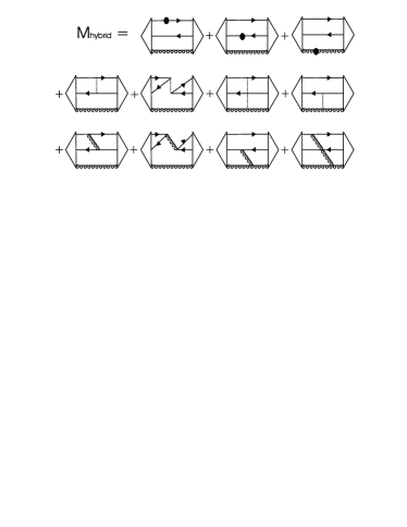
Figure 3: Diagrams for $\langle\Psi^{JPC}|H_{\rm eff}|\Psi^{JPC}\rangle$.

In the above expressions, $\epsilon_{\boldsymbol{q}}$, $\epsilon_{{\boldsymbol{\overline{q}}}}$ and $\varepsilon^{\mu\mu^{\prime}}_{\boldsymbol{g}}$ are the quark, anti-quark and gluon self-energies, respectively, evaluated at the indicated momentum (${\boldsymbol{g}=-\boldsymbol{q}-{\boldsymbol{\overline{q}}}}$). A pictorial representation for each type of contribution is given by the Feynman diagrams in Fig. 3.

The above expectation values are then computed variationally using the separable radial wavefunction, $F(q_{+},q_{-})=f(q_{+},\alpha_{+})f(q_{-},\alpha_{-})$, having two variational parameters, $\alpha_{+}$ and $\alpha_{-}$. We investigated two functional forms for $f$; a gaussian and a scalable, numerical solution from our two body meson studies. In general, the gaussian radial wavefunction,

$$f(q_{\pm},\alpha_{\pm})=e^{-x^{2}_{\pm}},\;\;x_{\pm}=\frac{q_{\pm}}{\alpha_{\pm}}$$ (45)

provided better results (lower variational mass) for s-wave states when compared to the numerical one. This was also true for p-wave orbital excitations, provided the gaussian was multiplied by $x_{\pm}$ corresponding to $l_{\pm}=1$. All integrals were calculated using the Monte Carlo method with the adaptive sampling algorithm VEGAS Vegas . The integrals were evaluated several times with an increasing number of points until a weight-averaged result converged. The hybrid mass error introduced by this procedure is about $\pm$50 MeV. For each $J^{PC}$ hybrid state we optimized the variational parameters $\alpha_{+}$ and $\alpha_{-}$ to produce the lowest mass. In terms of the string tension, their values fell in the ranges $0.9\sqrt{\sigma}\leq\alpha_{+}\leq 1.7\sqrt{\sigma}$ and $1.0\sqrt{\sigma}\leq\alpha_{-}\leq 3.3\sqrt{\sigma}$.

VI Results: Hybrid Meson Spectrum

VI.1 Light hybrid mesons

For the light hybrid calculation we used $m=$ 5 MeV PDG for the $u/d$ current quark mass. Results are listed in Table 3 which shows the ground state is the $0^{++}$ non-exotic scalar, followed by the triplet $1^{+-}$, $2^{++}$ and $1^{++}$. The lightest hybrid mass is 2.1 GeV.

For exotic states, as can be seen from Table 2, at least one p-wave in ${\boldsymbol{q}}_{+}$ or ${\boldsymbol{q}}_{-}$ is required. Because the $q\bar{q}$ interaction is repulsive for quarks in a color octet state, the excitation energy is less for a $l_{+}$ (gluon orbital) excitation than a $l_{-}$ ($q\bar{q}$ orbital) excitation since the quarks are further separated and experience a larger repulsive linear force.

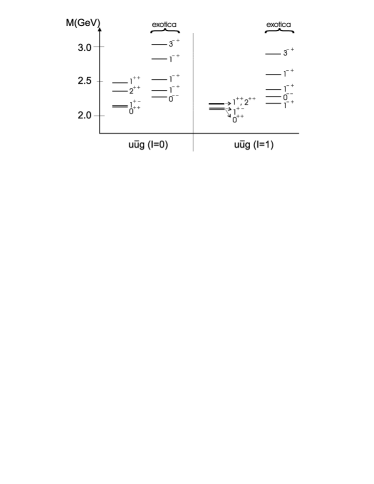
Figure 4: $u\overline{u}g$ spectrum.

$(I)J^{PC}$	$M_{J^{PC}}$ (MeV)	$M_{J^{PC}}$ (MeV)
	no corrections	with $g^{2}$ corrections
$(0)0^{++}$	2080	2135
$(1)0^{++}$	2065	2100	Ground
$(0)1^{+-}$	2135	2140	∗
$(1)1^{+-}$	2135	2140	∗
$(0)2^{++}$	2340	2335
$(1)2^{++}$	2180	2170
$(0)1^{++}$	2415	2470
$(1)1^{++}$	2110	2170
$(0)1^{-+}$	2500	2525	Exotic
$(1)1^{-+}$	2205	2220	Exotic
$(0)0^{--}$	2275	2280	Exotic
$(1)0^{--}$	2280	2285	Exotic
$(0)1^{-+}$	2370	2400	Exotic ∗
$(1)1^{-+}$	2370	2400	Exotic ∗
$(0)1^{-+}$	2760	2790	Exotic
$(1)1^{-+}$	2570	2600	Exotic
$(0)3^{-+}$	3030	3040	Exotic
$(1)3^{-+}$	2910	2915	Exotic

Table 3: Spectrum of light hybrid meson states. Error $\approx\pm$ 50 MeV. ^∗Isospin degenerate states.

The lightest exotic state is the $I=1,1^{-+}$, with mass 2.22 GeV. This is slightly higher than the Flux Tube model and lattice QCD predicted masses for this state which were between 1.7 and 2.1 GeV (see Table 1).

We studied the effects from including the non-abelian (NA) and hyperfine corrections for several states. Generally, both effects were small (except the hyperfine correction for charmed quarks, see below), roughly of the same order as the overall 50 MeV Monte Carlo error. In particular, the NA correction entailed several terms with different signs which tended to cancel.

Our model exotic spectrum (see Fig. 4) spans almost a GeV, between 2.1 and about 3 GeV, and includes predictions for $J$ up to 3. There are no exotic $J=$ 2 model states in this region since they require a d-wave or two p-waves, both involving much higher excitations.

Finally, we comment on an interesting isospin splitting effect. From Fig. 3, annihilation terms only contribute to the hybrid mass if the $q\overline{q}$ pair has quantum numbers consistent with the interaction. This is satisfied when $I_{q\overline{q}}=0$ and $S=1$. The annihilation diagrams can increase the $I=0$ hybrid states by several hundred MeV, as detailed in Table 3. In other cases, the $1^{+-}$ and one of the $1^{-+}$ states should be isospin degenerate, as we compute to within the Monte Carlo error. On the other hand, the states $0^{++}$ and $0^{--}$ are not expected to be degenerate but, within the error, they are. It may be that the isospin splitting is not zero, but rather is smaller than the numerical error. Note the annihilation process for s-wave, isoscalar quarks in a triplet spin state is analogous to $e^{-}e^{+}$ annihilation in the triplet state of positronium.

VI.2 Strange hybrid mesons

Table 4 summarizes results obtained for the $s\bar{s}g$ (hidden strangeness) hybrid mesons using a bare strange quark mass of 80 MeV. Now, the ground state is given by the non-exotic pseudovector state $1^{+-}$, with a 2.125 GeV mass, not at all reflecting the 75 MeV additional quark flavor mass contribution (the hybrid calculation is only sensitive to current quark masses above 200 MeV). Our prediction is in good agreement with the Flux Tube model and slightly above the only lattice prediction (see Table 1). In the exotic sector, the lightest state is given by $0^{--}$, with mass 2.3 GeV. Although there are also hybrid states with explicit strangeness, e.g. $s\bar{u}g$, we do not show predictions since the effect from the $s/u$ quark mass difference is small.

$J^{PC}$	$M_{J^{PC}}$ (MeV)	$M_{J^{PC}}$ (MeV)
	no corrections	with $g^{2}$ corrections
$1^{+-}$	2095	2125	Ground
$0^{++}$	2045	2140
$2^{++}$	2290	2315
$1^{++}$	2325	2420
$1^{-+}$	2350	2395	Exotic
$0^{--}$	2270	2300	Exotic
$1^{-+}$	2440	2485	Exotic
$1^{-+}$	2760	2820	Exotic
$3^{-+}$	2995	3030	Exotic

Table 4: Spectrum of $s\bar{s}g$ states. Error $\approx\pm$ 50 MeV.

$J^{PC}$	$M_{J^{PC}}$ (MeV)	$M_{J^{PC}}$ (MeV)
	no corrections	with $g^{2}$ corrections
$1^{+-}$	3310	3830	Ground
$0^{++}$	3295	3945
$2^{++}$	3410	3965
$1^{++}$	3450	4100
$1^{-+}$	3545	4020	Exotic
$0^{--}$	3510	4020	Exotic
$1^{-+}$	3590	4155	Exotic
$1^{-+}$	3985	4565	Exotic
$3^{-+}$	4065	4615	Exotic

Table 5: Spectrum of $c\bar{c}g$ states. Error $\approx\pm$ 50 MeV.

VI.3 Heavy hybrid mesons

Table 5 shows the results for the $c\bar{c}g$ (charmonium) hybrid mesons using a charmed quark mass of 1.0 GeV. The ground state is given, again, by the $1^{+-}$ state, with mass 3.83 GeV, while the lightest exotic hybrid lies at 4.02 GeV. These numbers are in reasonable agreement with previous lattice and Flux Tube predictions, as listed in Table 1.

Note that the correction introduced in the charmed case by the $g^{2}$ terms is roughly 500 to 600 MeV, significantly higher than in the lighter hybrid systems where the average corrections are 25 to 50 MeV. This large effect arises from the hyperfine correction to the quark and anti-quark self-energies (see Eqs. (IV, 40)), which is enhanced for heavier quark masses as discussed further in Ref. LCSS . Related, and as illustrated in Fig. 5, the charmonium hybrid spectrum now has a slightly different level ordering from the lighter hybrid spectra.

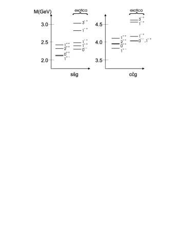
Figure 5: Low lying $s\overline{s}g$ and $c\overline{c}g$ spectra.

VI.4 Sensitivity to potential and parameters

One of our key findings using the Cornell potential is that the mass of the lightest hybrid, especially the exotic $1^{-+}$, is above 2 GeV. Because of the ramifications of this result for exotic state searches, we have performed an interaction sensitivity study by varying both potential forms and parameters.

We first varied the parameters in the Cornell potential to obtain a lower bound for our predicted exotic hybrid mass. Results are shown in Table 6 for different Coulomb potential parameters, $\alpha_{s}$, and string tensions, $\sigma$, found in the literature. For any combination of values consistent with previous studies LC1 ; LC2 ; LCSS ; LBC it was not possible to reduce the light hybrid mass to 1600 MeV. In particular, we tried $0.0\leq\alpha_{s}\leq 0.4$ and 367 MeV $\leq\sqrt{\sigma}\leq 424$ MeV. Indeed, to obtain a hybrid mass as low as 1600 MeV required an unphysical $\sqrt{\sigma}=$262 MeV.

potential/parameters	$I=1$ $u\bar{d}g$ hybrid	$c\bar{c}g$ hybrid
Cornell [Eq. (15)]
$\sqrt{\sigma}=367\,{\rm MeV},\;\alpha_{s}=0.4$	2220	4155
$\sqrt{\sigma}=367\,{\rm MeV},\;\alpha_{s}=0.2$	2390	4415
$\sqrt{\sigma}=367\,{\rm MeV},\;\alpha_{s}=0.0$	2540	4645
$\sqrt{\sigma}=424\,{\rm MeV},\;\alpha_{s}=0.4$	2555	4525
Renormalized [Eq. (18)]
$m_{g}=526\,{\rm MeV}$	2705	4730
$m_{g}=607\,{\rm MeV}$	3010	5130

Table 6: Calculated light and charmonium hybrid $1^{-+}$ masses, in GeV, using different interactions.

Table 6 also lists predictions for the confining potential given by Eq. (18) for values of the parameter $m_{g}=\sqrt{8\pi\sigma/12.25}$ corresponding to the two different Cornell string tensions $\sigma$ but with the same current quark masses ($m_{u}=$ 5 MeV, $m_{c}=$ 1 GeV). Note that this interaction yields $u\bar{d}g$ and $c\bar{c}g$ hybrids that are heavier than those given by the Cornell potential. Most significantly, this potential also predicts the lightest exotic hybrid has mass above 2 GeV. If we use $m_{c}=$ 0.85 GeV, which provides a reasonable description of the charmonium spectrum, the $1^{-+}$ $c\bar{c}g$ mass decreases to 4815 MeV for $m_{g}=$ 607 MeV.

VII Searching for hybrid mesons

Discovering exotic hadrons is a major goal motivating the Jefferson Lab 12 GeV upgrade and is also being actively pursued by other collaborations and facilities, such as Babar, Belle, RHIC, etc. For low energy investigations of light quark exotic systems there is, unfortunately, no clean energy scale demarkation, since $\Lambda_{QCD}$ governs the momentum distributions in light mesons and the strange quark mass is of the same order of magnitude. The obvious detection strategy is therefore to perform statistically accurate cross sections measurements to extract partial wave amplitudes with explicitly exotic quantum numbers not accessible to ordinary $q\bar{q}$ states. However for (hidden) exotics with conventional meson quantum numbers, it will be difficult to establish their nature. Note certain Flux Tube model Barnes and lattice predictions indicate that p-wave hybrid mesons prefer to decay to hadron pairs with one hadron also having a p-wave, rather than to two s-wave hadrons with a relative motion p-wave, e.g. $\eta h_{1}$ in an s-wave as opposed to $\pi\pi$ in a p-wave. It will be interesting to check this prediction experimentally.

More germane to the results of this paper are high energy experiments where novel tests can be conducted based on the scale separation provided by either the high beam energy or the heavy quark mass. This is discussed in the next two subsections.

VII.1 Application of dimensional counting rules

Dimensional counting rules Brodsky predict a power-law production cross section behavior for a given state at asymptotically high energies. They are based on the requirement that in forming a bound state with an energetic quark, the other partons must acquire very small relative momenta consistent with the production hadron’s internal momentum distribution. This becomes highly unlikely in energetic collisions and therefore the production cross section falls as a power law, with the exponent increasing with increasing minimum number of constituents. For a hidden hybrid, the wavefunction has the Fock space expansion

$$\arrowvert\psi\rangle=\beta_{1}\arrowvert{c\bar{c}}\rangle+\beta_{2}\arrowvert{c\bar{c}g}\rangle+\cdot\cdot\cdot$$ (46)

where the quantum numbers are conventional but the first coefficient $\beta_{1}$ is presumably small. Therefore the power-law behavior will reveal the second term in this series and permit distinguishing this exotic meson from ordinary $c\bar{c}$ charmonium (same for bottomonium). To be specific in the following discussion we focus on the recently discovered $\psi(4260)$ whose nature is currently under debate. The same remarks apply to any other hidden hybrid meson candidate.

Inclusive production

First consider the inclusive production reaction $e^{-}e^{+}\to\psi+X$. The virtual photon fragments into a $c\bar{c}$ pair, each carrying half of the total center of mass momentum and therefore each has an energy equal to the beam energy $E_{beam}$ (in a symmetric collider). The dimensional counting rules apply in the limit in which the produced particle’s energy approaches its threshold value, that is,

$$x=\frac{E_{\psi}}{E_{beam}}\to 1\ .$$ (47)

In this limit, the power law behavior for a conventional charmonium state is $1-x$ and for a hybrid state with a minimum of one more gluon constituent in the leading wavefunction, $(1-x)^{3}$ Gunionplb79 . That is, as the $\psi$ is produced with more energy (this can be determined kinematically), the production cross section decreases linearly towards the kinematical endpoint where the $\psi$ has the maximum available energy. Note that the hybrid production cross section decreases even more rapidly as a cubic polynomial. With a sufficient number of events this can be documented experimentally.

Exclusive production

Bodwin, Braaten and Lee Bodwinprl have recently examined the reaction $e^{-}e^{+}\to\psi\psi$. Their study focused on the ground state $J/\psi$, but their arguments also apply to the production of excited vector charmonia or a $J/\psi$ accompanied by a $\psi(4260)$. They studied $\psi\psi$ production as a function of the (small) variable ( $m_{c}$ is the charmed quark mass)

$$r=\frac{m_{c}}{E_{beam}}$$

and find in the limit $r\to 0$, the differential cross section at fixed angle is constant. However, a straight-forward counting rule application predicts the production cross section is suppressed by a power of $s$ or, equivalently, two powers of $r$, if one of the two produced hadrons is predominantly a hybrid meson, that is

$$\frac{d\sigma}{d\cos\theta} \simeq {\rm constant}\ ,\;\;{\rm for}\;c\bar{c}$$ (48)

$$\frac{d\sigma}{d\cos\theta} \simeq \frac{\rm constant}{r^{2}}\ ,\;\;{\rm for}\;c\bar{c}g\ .$$ (49)

Establishing this behavior only requires measuring double charmonium production at three sufficiently high energies. For non-vector mesons both cross sections are further suppressed by additional powers of $r$, but the extra $r^{2}$ signature always marks the presence of one more constituent, and therefore tags the hybrid meson. This argument also applies to the production of light hybrids in high-energy electron-positron colliders.

To conclude this subsection, we note that the power-law predictions can be modified by QCD logarithms at very high energies and that in the strict limit $r\to 0$ or $x\to 0$, any $c\bar{c}$ admixture in the wavefunction would dominate production. However for current, available low energies, the production will still be dominated by the hybrid component if $\beta_{1}<<\beta_{2}$, i.e. if a predominantly pure hybrid state is found.

VII.2 Distinguishing the hybrid from charmonium

In this subsection we propose a novel method applicable to the decay of heavy quarkonium that enables identifying a new state as either a radial excitation of conventional charmonium or a hybrid state. The method is based upon two key points.

First, we note that, due to the gluon mass gap scale, a conventional $q\bar{q}$ ground state (e.g. a well established $J/\psi$ or $\Upsilon$, etc.) is lighter than a $q\bar{q}g$ ground state hybrid with the same flavor. Indeed, the ground state hybrid mass is more comparable to a radially excited quarkonium state. For example in our approach the $\psi(4s)$ and the ground state vector $c\bar{c}g$ state have similar masses. Now different eigenstates of a hermitian Hamiltonian are orthogonal with the $n$th radial excited state having $n-1$ nodes. Therefore, even though the total energies (masses) are similar, the relative momentum distribution of the quarks in excited charmonium looks quite different from the quark momentum distribution in the ground state hybrid (see Figs. 6 and 7).

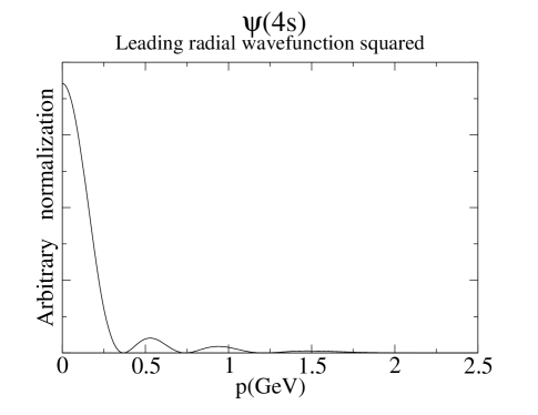
Figure 6: Probability density, $\arrowvert\psi(p)\arrowvert^{2}$, for the 4s charmonium state. This is the relative $c\bar{c}$ quark momentum distribution.

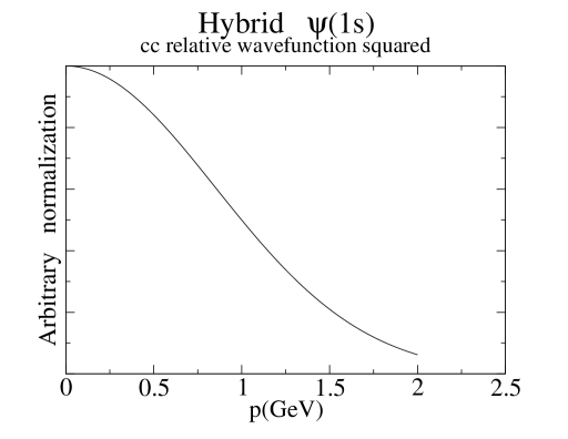
Figure 7: Typical quark relative momentum distribution in a $c\bar{c}g$ hybrid state with a mass near 4300 MeV. The extra mass energy, relative to a $c\bar{c}$ $J/\psi$, corresponds to gluon field excitations in collective models such as the Flux Tube approach or in the quasi-particle (gluon) mass gap in the constituent picture, but not in nodal radial excitation for the relative $c\bar{c}$ motion (compare to the radially excited charmonium distribution in Fig. 6).

The second point involves the Franck-Condon (FC) principle widely used in molecular physics. Franck and Condon were the first to appreciate that molecular electronic transitions proceed too rapidly for the much heavier nuclei to respond. The FC principle is applicable whenever there is a mass scale separation between different particles. In the context of quarkonium this means that the light fields (pions, gluons, etc.) quickly rearrange and the heavy quarks do not appreciably change their momentum distribution in the decay. Hence, the relative momentum between the decay products directly correlates with the quark momentum distribution in the parent quarkonium. Unfortunately in the simplest 2-body decays such as

$$\psi(ns)\to D\bar{D},\ \ \Upsilon(ns)\to B\bar{B}$$

the FC constraint is not relevant since in the center of mass frame the momentum of the final products is fixed. This leads to smaller wavefunction overlaps suppressing the decay somewhat. However in 3-body decays such as

$$\psi(ns)\to D\bar{D}\pi,\ \ \Upsilon(ns)\to B\bar{B}\pi\ ,$$

the FC constraint applies. The first reaction can be employed to study the recently discovered $\psi(4260)$. The second will be useful in an envisioned Belle collaboration measurement to establish whether this excited bottomonium state is the predicted quark model 5s meson state.

Thus, we contend that the relative momentum distribution between the $D$ and $\bar{D}$ mesons in the $D\bar{D}\pi$ system mirrors the momentum distribution of the quarks in the parent $\psi$ meson. Since the hybrid ground state wavefunction does not have a node, the resulting momentum distribution for the $D\bar{D}$ subsystem is also node-less and thus smoother than that for a conventional radially excited charmonium. Multiplying by the relevant phase space distribution for this decay, yields the momentum distribution in Fig. 8 that can be observed experimentally in the heavy-quark limit. The maximum is in the mid-momentum region where phase-space is larger and the wavefunction is near a local maximum.

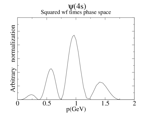
Figure 8: Momentum distribution of Fig. 6 multiplied by the phase space for the decay $\psi(4260)\to D\bar{D}\pi$. This is the probability density for finding a $D\bar{D}\pi$ state with relative $D\bar{D}$ momentum $p$ according to the Franck-Condon principle in the heavy-quark limit. This signature will be more robust for the related bottomonium process $\Upsilon(5s)\to B\bar{B}\pi$.

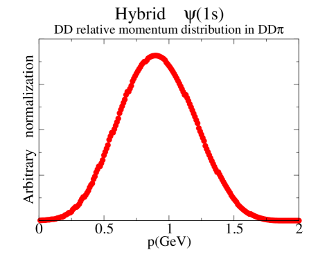
Figure 9: The relative momentum distribution of the $D\bar{D}$ pair in the $D\bar{D}\pi$ final state for a charmed hybrid meson with momentum distribution given in Fig. 7. The distribution of the final products has a smooth bell shape in sharp contrast to the radially excited quarkonium distribution in Fig. 10.

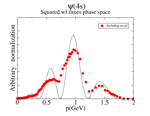
Figure 10: The momentum distribution in Fig. 8 (solid line) and the distribution (dots) obtained averaging over a 150 MeV spread to approximate the actual quark momentum distribution in the $D$ meson. The experimental signal, firmer for bottomonium than charmonium, is a central peak with two shoulders for the relative momentum distribution of the $B\bar{B}$ (or $D\bar{D}$) pair in the $B\bar{B}\pi$ (or $D\bar{D}\pi$) final state. These adjacent enhancements identify the resonance as a radially excited quarkonium state as opposed to a hybrid meson.

However, since quarks are not infinitely heavy, the FC signature is modified due to the recoil of the quarks in the $D$ meson, yielding a different momentum distribution. For example, taking a quark relative momentum between 150 and 200 MeV, one obtains the $c\bar{c}g$ momentum distribution illustrated in Fig. 9 for the ground state vector hybrid, and the smeared final state $D\bar{D}$ momentum distribution plotted in Fig. 10 for radially excited charmonium. As can be seen, even after smearing, there is still residual structure information adjacent to the central peak for radially excited charmonium that is reminiscent of its parent charmonium wavefunction behavior, in sharp contrast to the smooth, bell-shaped hybrid distribution.

We therefore advocate analyzing the $D\bar{D}$ and $B\bar{B}$ relative momentum distributions in $D\bar{D}\pi$ and $B\bar{B}\pi$ decays of highly excited quarkonia. Additional final state pions or other light particles do not alter our arguments (but restrict somewhat the available phase space), so there are several other possible final state channels to search.

VIII Discussion and Conclusions

Our key model predictions are that the lightest hybrid mass is 2.1 GeV, with the lightest $1^{-+}$ exotic state slightly above 2.2 GeV. Lattice and Flux Tube calculations yield a mass of at least 1.8 GeV for the $1^{-+}$, except Ref. Hedditch which predicts a mass around 1.7 GeV. Thus, with exception to this last work, the composite model analyses appear to preclude the possibility of the reported $1^{-+}$ exotica, $\pi_{1}(1400)$ and $\pi_{1}(1600)$, being hybrid mesons. If this is correct, one should investigate other structures for those two hadrons, such as tetraquark molecules, with both $q\overline{q}$ pairs in color singlets, or tetraquark atoms, where quark pairs are in intermediate non-singlet color states and we are currently applying our model to these systems. However, if the lattice 1.7 GeV $1^{-+}$ prediction is robust, one can not yet exclude the observed $\pi_{1}(1600)$ from being a hybrid, but this still does not explain the structure of the $\pi_{1}(1400)$. It would be very useful to have other lattice measurements, using the same techniques as Ref. Hedditch , to confirm or reject this result. Related, we have also varied our model parameters and potential forms to obtain a lower bound for our predicted exotic hybrid mass which is clearly above 2 GeV.

Regarding isospin splitting, our results show an enhanced splitting from $g^{2}$ corrections. For the $0^{++}$ hybrid, the corrections increased the splitting from 15 to 35 MeV, the maximum increase in the light hybrid spectrum.

In the strange sector, we predict the lightest non-exotic hybrid mass is 2.125 GeV, while the lightest exotic mass is 2.30 GeV. These values compare reasonably well with Flux Tube Barnes ; Close ; Katja and, slightly lighter, lattice Hedditch results. For the charmed sector, our predictions of 3.83 GeV for the lightest hybrid and 4.02 GeV for the lowest exotic are also in good agreement with several other lattice and Flux Tube studies (see Table 1).

As mentioned above, the different $g^{2}$ corrections produced an overall small effect, about the same order as the Monte Carlo error. However, the hyperfine correction becomes important for heavier quark mass. In the charmed sector, this correction added about 500 to 600 MeV to the hybrid mass. Lastly, note the level ordering of the exotic isoscalar $u\overline{u}g$ and $s\overline{s}g$ spectra are the same, $0^{--}$, $1^{-+}$, $1^{-+}$, $1^{-+}$ and $3^{-+}$, but slightly different than the exotic $c\overline{c}g$ system, where the $0^{--}$ and lowest $1^{-+}$ are degenerate. This is a consequence of the enhanced charmonium self-energy from the hyperfine interaction.

Finally, we discussed both low and high energy scenarios for observing hybrid mesons. For low energy studies involving light quark systems, dimensional counting rules predict specific power-law behaviors for distinguishing between production of conventional and hybrid mesons. For high energy investigations of heavy quark systems, the Frank-Condon principle provides a useful constraint on the final state momentum distributions which should assist experimentalist in identifying heavy hybrid systems.

In summary, lattice, Flux Tube and our $H_{\rm eff}$ many-body approach all predict similar hybrid spectra and that the lightest $1^{-+}$ exotic hybrid meson mass is near 2 GeV. This composite model agreement indicates that the $\pi_{1}(1600)$ is not a hybrid meson but has an alternative structure. If true and if the $\pi_{1}(1600)$ exists, it is more likely a tetraquark system, either a $(q\overline{q})$ $(q\overline{q})$ meson molecule or an exotic $qq\bar{q}\bar{q}$ atom. Future work will apply our model to light and heavy tetraquark systems including mixing with hybrid and conventional meson states. Three-body forces Szczepaniak:2006nx will also be examined.

- (1) D. Alde et al., Phys. Lett. B 205, 397 (1988).
- (2) D. R. Thompson et al. (E852 Collaboration), Phys. Rev. Lett. 79, 1630 (1997).
- (3) S. U. Chung et al. (E852 Collaboration), Phys. Rev. D 60, 092001 (1999).
- (4) G. S. Adams et al. (E852 Collaboration), Phys. Rev. Lett 81, 5760 (1998).
- (5) S. U. Chung et al. (E852 Collaboration), Phys. Rev. D 65, 072001 (2002).
- (6) A. R. Dzierba et al., Phys. Rev. D 73, 072001 (2006).
- (7) D. V. Amelin et al. (VES Collaboration), Phys. Lett. B 356, 595 (1995).
- (8) A. Zaitsev, AIP Conf. Proc. 432, 461 (1998).
- (9) A. Donnachie and Yu. S. Kalashnikova, Phys. Rev. D 60, 114011 (1999).
- (10) K. Karch et al. (Crystal Ball Collaboration), Z. Phys. C 54, 33 (1992).
- (11) J. Adomeit et al. (Crystal Barrel Collaboration), Z. Phys. C 71, 227 (1996).
- (12) D. Barberis et al. (WA102 Collaboration), Phys. Lett. B 413, 217 (1997).
- (13) Yu. S. Kalashnikova, Nucl. Phys. A689, 49 (2001).
- (14) F. Buisseret and V. Mathieu, arXiv:hep-ph/0607083.
- (15) C. Bernard et al., Phys. Rev. D 56, 7039 (1997).
- (16) C. Bernard et al., Nucl. Phys. (Proc. Suppl.) B73, 264 (1999).
- (17) P. Lacock and K. Schilling, Nucl. Phys. (Proc. Suppl.) B73, 261 (1999).
- (18) J. N. Hedditch et al., Phys. Rev. D 72, 114507 (2005).
- (19) X. Q. Luo and Z. H. Mei, Nucl. Phys. (Proc. Suppl.) B119, 263 (2003).
- (20) T. Barnes, F. E. Close and E. S. Swanson, Phys. Rev. D 52, 5242 (1995).
- (21) F. E. Close and P. R. Page, Nucl. Phys. B443, 233 (1995).
- (22) K. Waidelich, Diploma Thesis, North Carolina State University (2001).
- (23) T. Barnes, Ph.D. Thesis, Caltech (1977); Nucl. Phys. B158, 171 (1979); T. Barnes and F. Close, Phys. Lett. B 116, 365 (1982); M. Chanowitz and S. Sharpe, Nucl. Phys. B222, 211 (1983); T. Barnes et al., Nucl. Phys. B224, 241 (1983); M. Flensburg et al., Z. Phys. C 22, 293 (1984); P. Hasenfratz et al., Phys. Lett. B 95, 299 (1980).
- (24) F. Iddir and L. Semlala, arXiv:hep-ph/0511086.
- (25) Y. Liu and X. Q. Luo, Phys. Rev. D 73, 054510 (2006).
- (26) L. A. Griffiths, C. Michael and P. E. L. Rakow, Phys. Lett. B 129, 351 (1983).
- (27) S. Perantonis and C. Michael, Nucl. Phys. B347, 854 (1990).
- (28) F. J. Llanes-Estrada and S. R. Cotanch, Nucl. Phys. A697, 303 (2002).
- (29) F. J. Llanes-Estrada, S. R. Cotanch, A. P. Szczepaniak and E. S. Swanson, Phys. Rev. C 70, 035202 (2004).
- (30) F. J. Llanes-Estrada, P. Bicudo and S. R. Cotanch, Phys. Rev. Lett. 96, 081601 (2006).
- (31) F. J. Llanes-Estrada and S. R. Cotanch, Phys. Rev. Lett. 84, 1102 (2000).
- (32) F. J. Llanes-Estrada and S. R. Cotanch, Phys. Lett. B 504, 15 (2001).
- (33) T. D. Lee, Particle Physics and Introduction to Field Theory (Harwood Academic Publishers, New York, 1990).
- (34) A. P. Szczepaniak and E. S. Swanson, Phys. Rev. D 65, 0252012 (2002).
- (35) G. P. Lepage, Journal of Comput. Phys. 27, 192 (1978); Cornell University Report CLNS 80-447, 1980 (unpublished).
- (36) S. Eidelman et al., Phys. Lett. B 592, 1 (2004).
- (37) S. J. Brodsky and G. R. Farrar, Phys. Rev. Lett. 31, 1153 (1973); Phys. Rev. D 11, 1309 (1975).
- (38) J. F. Gunion, Phys. Lett. B 88, 150 (1979).
- (39) G. T. Bodwin, E. Braaten and J. Lee, Phys.Rev. D 72, 014004 (2005).
- (40) A. P. Szczepaniak and P. Krupinski, Phys. Rev. D 73, 116002 (2006).