KA–TP–09–2006

hep-ph/0609075

Anomalous Higgs boson couplings in vector boson fusion at the CERN LHC
V. Hankele, G. Klämke, D. Zeppenfeld Institut für Theoretische Physik, Universität Karlsruhe, P.O.Box 6980, 76128 Karlsruhe, Germany and T. Figy Institute of Particle Physics Phenomenology, University of Durham, Durham, DH1 3LE, UK

Deviations from SM expectations in the Higgs sector can be parameterized by an effective Lagrangian. The corresponding anomalous couplings have been implemented in a Monte Carlo program for Higgs production in vector boson fusion, at NLO QCD accuracy. It allows to study anomalous coupling effects for production and decay of the Higgs boson. We analyze deviations allowed by LEP data and study a new azimuthal angle variable which directly measures the interference between CP-even, CP-odd and SM couplings.

1 Introduction

At the LHC, the second most copious source for a standard model (SM) type Higgs boson is expected to be the vector boson fusion (VBF) channel, i.e. electroweak processes of the type $qq\to qqH$ [1, 2]. While the production cross section from gluon fusion is larger, VBF has the advantage of a richer kinematic structure with two forward tagging jets which result from the scattered quarks. The characteristic distributions of these forward and backward tagging jets allow for significant reduction of backgrounds which should result in fairly clean samples of signal events. These samples can then be used to measure properties of the Higgs boson, in particular its couplings to gauge bosons and fermions. This includes the magnitude of the couplings [3] but also the tensor structure of the $HVV$ vertex ($V=W,Z$) [4].

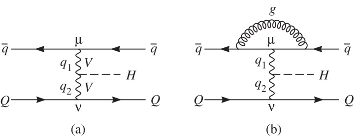
Figure 1: Feynman graphs contributing to $\bar{q}Q\to\bar{q}QH$ at (a) tree level and (b) including virtual corrections to the upper quark line. The momentum labels and Lorentz indices for the internal weak bosons correspond to the vertex function of Eq. (1.1).

The total cross section for Higgs production via VBF has been known at NLO QCD accuracy since the early nineties [5]. More recently, the NLO corrections to distributions have also been calculated, and are available in the form of NLO parton level Monte Carlo programs for a SM Higgs boson [6, 7] and also for a general tensor structure of the $HVV$ coupling [8], as depicted in Fig. 1. The most general tensor structure of the $HVV$ vertex which can contribute to VBF in the massless quark limit can be written as

$$T^{\mu\nu}(q_{1},q_{2})=a_{1}(q_{1},q_{2})\;g^{\mu\nu}+a_{2}(q_{1},q_{2})\;[q_{1}\cdot q_{2}g^{\mu\nu}-q_{2}^{\mu}q_{1}^{\nu}]+a_{3}(q_{1},q_{2})\;\varepsilon^{\mu\nu\rho\sigma}q_{1\rho}q_{2\sigma}\;.$$ (1.1)

A constant $a_{1}$ (with $a_{2}=0=a_{3}$) represents the SM case while sizable form factors $a_{2}$ and/or $a_{3}$ would represent new physics, induced, for example, by a heavy particle loop. Such new physics effects would, of course, not only change Higgs production cross sections but also the decay rates and branching ratios for $H\to VV$ ($V=W,Z,\gamma$). A convenient starting point for a consistent treatment of such correlated effects on production and decay is a description by an effective Lagrangian, which is constructed out of EW gauge fields and the SM Higgs doublet field in a $SU(2)\times U(1)$ gauge invariant way. The corresponding operators [10, 11] have been considered in the past for describing new physics contributions to Higgs physics, see e.g. [12, 13, 14]. They are described in Section 2. We have now incorporated these effects on Higgs decays into our VBFNLO program, which allows to simulate general VBF processes with NLO QCD accuracy [6, 9]. One purpose of the present paper is to make available this new simulation tool for Higgs signals at the LHC. We give a brief description of our program in Section 3.

The remainder of this paper analyzes signals of anomalous Higgs couplings in VBF processes at the LHC. Sizable effective $H\gamma\gamma$ and $HZ\gamma$ couplings of a sufficiently light Higgs boson would have led to $e^{+}e^{-}\to H\gamma$ events at LEP and are, hence, tightly constrained [16]. These constraints limit the maximal LHC signals. In Section 4 we analyze the implications for total Higgs production cross sections in VBF, we consider the effect on Higgs branching ratios, and we use our simulation tools to find distributions which are sensitive to small interference effects between the three different tensor structures of Eq. (1.1). Of particular interest here are distributions of the two (anti-)quark jets in VBF events. These forward and backward tagging jets are characteristic features of the VBF process and their distributions and correlations can be exploited to reveal information on the tensor structure of the $HVV$ vertex, independent of the Higgs decay mode. In Ref. [4] it was shown that the absolute value of the azimuthal angle between the two tagging jets can distinguish between the three different choices of tensor structures in Eq. (1.1). However, interference effects between the CP-even coupling $a_{2}$ and the CP-odd coupling $a_{3}$ cancel in this distribution, and results for $|a_{2}|=|a_{3}|$ are very close to SM predictions. Here we show that the azimuthal angle can be defined in such a way that also its sign can be determined at the LHC and that this new angle exhibits the interference between $a_{2}$ and $a_{3}$. Indeed, the ratio of the two form factors can be directly measured via the position of the minimum of the azimuthal angle distribution. Such interference effects would signal CP-violation in the Higgs sector. Conclusions are given in Section 5.

2 Effective Lagrangian and anomalous couplings

We are concerned with deviations in the $HV_{1}V_{2}$ couplings ($V_{i}=W,Z,\gamma$) from SM predictions, and, more generally, with new physics effects in the bosonic sector of the SM. A model-independent description of such effects is provided by an effective Lagrangian approach, where, in order to preserve the successful SM predictions for $W$ and $Z$ interactions with fermions, the SM $SU(2)\times U(1)$ gauge symmetry is taken as exact, albeit spontaneously broken. It is, hence, required for all higher dimensional operators in the effective Lagrangian [10],

$${\cal L}_{eff}={\cal L}_{SM}+\sum_{i}\frac{f_{i}^{(6)}}{\Lambda^{2}}{\cal O}_{i}^{(6)}+...\;.$$ (2.1)

With a scalar doublet field giving rise to the Higgs boson, an even number of covariant derivatives and of Higgs doublet fields is required which leaves operators of even dimensionality only. The relevant operators for our discussion are four CP-even and three CP-odd operators of dimension 6, namely

$$\begin{split}&{\cal O}_{BB}=\Phi^{+}\ \hat{B}_{\mu\nu}\hat{B}^{\mu\nu}\ \Phi\hskip 62.59596pt{\cal O}_{\tilde{B}B}=\Phi^{+}\ \hat{\tilde{B}}_{\mu\nu}\hat{B}^{\mu\nu}\ \Phi\\ &{\cal O}_{WW}=\Phi^{+}\ \hat{W}_{\mu\nu}\hat{W}^{\mu\nu}\ \Phi\hskip 51.21504pt{\cal O}_{\tilde{W}W}=\Phi^{+}\ \hat{\tilde{W}}_{\mu\nu}\hat{W}^{\mu\nu}\ \Phi\\ &{\cal O}_{B}=(D_{\mu}\Phi)^{+}\ \hat{B}^{\mu\nu}\ (D_{\nu}\Phi)\hskip 39.83368pt{\cal O}_{\tilde{B}}=(D_{\mu}\Phi)^{+}\ \hat{\tilde{B}}^{\mu\nu}\ (D_{\nu}\Phi)\\ &{\cal O}_{W}=(D_{\mu}\Phi)^{+}\hat{W}^{\mu\nu}\ (D_{\nu}\Phi).\end{split}$$ (2.2)

In this formula the covariant derivative, $D_{\mu}$, the field strength tensors, $\hat{B}_{\mu\nu}$ and $\hat{W}_{\mu\nu}$, of the W and B gauge fields and their dual ones are given by:

$$\begin{split}&D_{\mu}=\partial_{\mu}+\frac{i}{2}\ g^{\prime}\ B_{\mu}+i\ g\ \frac{\sigma^{a}}{2}\ W_{\mu}^{a},\\ &\hat{B}_{\mu\nu}+\hat{W}_{\mu\nu}=i\ \frac{g^{\prime}}{2}\ B_{\mu\nu}+i\ \frac{g}{2}\ \sigma^{a}\ W_{\mu\nu}^{a}=[D_{\mu},D_{\nu}]\\ &\tilde{V}_{\mu\nu}=\frac{1}{2}\ \epsilon_{\mu\nu\rho\sigma}\ V^{\rho\sigma},\qquad(V=B,\ W).\end{split}$$ (2.3)

Two other operators of dimension 6, ${\cal O}_{\Phi,1}=(D_{\mu}\Phi)^{+}\ \Phi\Phi^{+}\ (D^{\mu}\Phi)$ and ${\cal O}_{BW}=\Phi^{+}\ \hat{B}_{\mu\nu}\ \hat{W}^{\mu\nu}\ \Phi$, contribute to anomalous $HVV$ couplings, but have already been constrained strongly by electroweak high precision measurements [11, 15] and will be neglected in the following.

The notation we refer to is the one used by the L3 collaboration [16] with the effective Lagrangian

$$\begin{split}{\cal L}_{eff}^{(6)}\ &=\ g_{H\gamma\gamma}\ HA_{\mu\nu}A^{\mu\nu}\ +\ g_{HZ\gamma}^{(1)}\ A_{\mu\nu}Z^{\mu}\partial^{\nu}H+\ g_{HZ\gamma}^{(2)}\ HA_{\mu\nu}Z^{\mu\nu}\\ &+\ g_{HZZ}^{(1)}\ Z_{\mu\nu}Z^{\mu}\partial^{\nu}H+\ g_{HZZ}^{(2)}\ HZ_{\mu\nu}Z^{\mu\nu}+\ g_{HWW}^{(2)}\ HW_{\mu\nu}^{+}W_{-}^{\mu\nu}\\ &+\ g_{HWW}^{(1)}\ (W_{\mu\nu}^{+}W_{-}^{\mu}\partial^{\nu}H\ +\ W_{\mu\nu}^{-}W_{+}^{\mu}\partial^{\nu}H\ )+\ \tilde{g}_{H\gamma\gamma}\ H\tilde{A}_{\mu\nu}A^{\mu\nu}\\ &+\ \tilde{g}_{HZ\gamma}\ H\tilde{A}_{\mu\nu}Z^{\mu\nu}+\ \tilde{g}_{HZZ}\ H\tilde{Z}_{\mu\nu}Z^{\mu\nu}+\ \tilde{g}_{HWW}^{(2)}\ H\tilde{W}_{\mu\nu}^{+}W_{-}^{\mu\nu}.\end{split}$$ (2.4)

The $g_{HVV}$ are coefficients of the CP-even and the $\tilde{g}_{HVV}$ the ones of the CP-odd operators. $g_{HZ\gamma}^{(1)}$, $g_{HZZ}^{(1)}$ and $g_{HWW}^{(1)}$ can be parameterized using the well known coefficients of the anomalous triple gauge boson couplings, $\triangle\kappa_{\gamma}$ and $\triangle g_{1}^{Z}$  [17]. They are already highly restricted by a combination of the measurements of the four LEP collaborations [18]. The CP-odd coefficients $\tilde{g}_{HZ\gamma}$ and $\tilde{g}_{HZZ}$ depend on the parameter $\tilde{\kappa}_{\gamma}$, which has also been constrained in the past by LEP data [19]. The remaining coefficients depend on two parameters,

$$d=-\frac{m_{W}^{2}}{\Lambda^{2}}\ f_{WW},\hskip 85.35826ptd_{B}=-\frac{m_{W}^{2}}{\Lambda^{2}}\ \frac{\sin^{2}{\theta_{w}}}{\cos^{2}{\theta_{w}}}\ f_{BB}$$ (2.5)

for the CP-even and completely analogous on $\tilde{d}$ and $\tilde{d}_{B}$ for the CP-odd couplings.

$$\begin{split}&g_{H\gamma\gamma}=\frac{g}{2\ m_{W}}\ (d\ \sin^{2}{\theta_{w}}+d_{B}\ \cos^{2}{\theta_{w}})\hskip 142.26378pt\\ &g_{HZ\gamma}^{(2)}=\frac{g}{2\ m_{W}}\ \sin{2\theta_{w}}\ (d-d_{B})\\ &g_{HZZ}^{(2)}=\frac{g}{2\ m_{W}}\ (d\ \cos^{2}{\theta_{w}}+d_{B}\ \sin^{2}{\theta_{w}})\\ &g_{HWW}^{(2)}=\frac{g}{m_{W}}\ d.\end{split}$$ (2.6)

The best constraints for the parameters $d$ and $d_{B}$ come from the L3 collaboration. They are really bounds on $g_{H\gamma\gamma}$ and $g_{HZ\gamma}^{(2)}$, which have been derived using the L3 bounds on the Higgs partial widths $\Gamma(H\to\gamma\gamma)$ and $\Gamma(H\to Z\gamma)$ of Fig. 7(a) in Ref. [16]. For these couplings and also for $d$ and $d_{B}$, the strongest constraints are from the unsuccessful search for the process $e^{+}e^{-}\to H\gamma\to\gamma\gamma\gamma$ via photon or $Z$-boson exchange in Higgs production. Direct bounds on $g_{HZZ}^{(2)}$ can only be derived from the process $e^{+}e^{-}\to HZ$ and, thus, for Higgs masses below $\approx 114$ GeV.

Table 1: Approximate direct 95 % CL bounds for $g_{H\gamma\gamma}$ and $g^{(2)}_{HZ\gamma}$ in $[\mathrm{TeV}^{-1}]$. They are derived from the partial decay width bounds of Ref. [16].

Higgs mass	$g_{H\gamma\gamma}$	$g^{(2)}_{HZ\gamma}$
120 GeV	$[-0.17,0.17]$	$[-1.24,1.24]$
140 GeV	$[-0.24,0.24]$	$[-1.35,1.35]$

Since the parameters $d$ and $d_{B}$ also appear in the other coefficients of Eq. (2.6), the L3 constraints can be used to estimate upper bounds for $g_{HZ\gamma}^{(2)}$, $g_{HZZ}^{(2)}$ and $g_{HWW}^{(2)}$. The best indirect bounds are summarized in Table 2 and Table 3. The parameter $d_{B}$ is stronger constrained than $d$ because in $g_{H\gamma\gamma}$ they appear in the combination $d_{B}\cdot\cos^{2}{\theta_{w}}$ and $d\cdot\sin^{2}{\theta_{w}}$. Since $\cos^{2}{\theta_{w}}\approx 3\cdot\sin^{2}{\theta_{w}}$ this means that the best bounds on $d_{B}$ are about three times better than for $d$. Below we shall use the maximal values of the $g_{HVV}$ induced by a pure $d$ coupling, i.e. the ${\cal O}_{WW}$ operator, to estimate maximal allowed deviations from the SM which might arise from anomalous $HVV$ couplings.

Table 2: The best indirect 95 % CL constraints of the L3 collaboration [16] for $g_{H\gamma\gamma}$, $g^{(2)}_{HZ\gamma}$, $g^{(2)}_{HZZ}$ and $g^{(2)}_{HWW}$ in $[\mathrm{TeV}^{-1}]$, assuming $SU(2)\times U(1)$ invariant dimension 6 effective couplings with $d_{B}=0$.

Higgs mass	$g_{H\gamma\gamma}$	$g^{(2)}_{HZ\gamma}$	$g^{(2)}_{HZZ}$	$g^{(2)}_{HWW}$
120 GeV	$[-0.16,0.16]$	$[-0.59,0.59]$	$[-0.54,0.54]$	$[-1.41,1.41]$
140 GeV	$[-0.24,0.22]$	$[-0.86,0.79]$	$[-0.78,0.72]$	$[-2.04,1.88]$
150 GeV	$[-0.31,0.29]$	$[-1.12,1.01]$	$[-1.02,0.96]$	$[-2.66,2.51]$
160 GeV	$[-0.47,0.37]$	$[-1.72,1.35]$	$[-1.57,1.23]$	$[-4.07,3.21]$

Table 3: The best indirect 95 % CL constraints of the L3 collaboration [16] for $g_{H\gamma\gamma}$, $g^{(2)}_{HZ\gamma}$, $g^{(2)}_{HZZ}$ and $g^{(2)}_{HWW}$ in $[\mathrm{TeV}^{-1}]$, assuming $SU(2)\times U(1)$ invariant dimension 6 effective couplings with $d=0$.

Higgs mass	$g_{H\gamma\gamma}$	$g^{(2)}_{HZ\gamma}$	$g^{(2)}_{HZZ}$
120 GeV	$[-0.18,0.18]$	$[-0.20,0.20]$	$[-0.05,0.05]$
140 GeV	$[-0.24,0.24]$	$[-0.26,0.26]$	$[-0.07,0.07]$
150 GeV	$[-0.27,0.27]$	$[-0.30,0.30]$	$[-0.08,0.08]$
160 GeV	$[-0.39,0.39]$	$[-0.43,0.43]$	$[-0.12,0.12]$

Although the L3 collaboration does not give the corresponding values for the CP-odd couplings they are implicitly constrained by existing data, because CP-even and CP-odd couplings give identical contributions to the differential cross section for $e^{+}e^{-}\to H\gamma$:

$$\frac{d\sigma}{d\Omega}\ (e^{+}e^{-}\to H\gamma)=\frac{\alpha^{2}}{8}\ (1-\frac{m_{H}^{2}}{s})^{3}\ (1+\cos^{2}{\theta})\ (F(s)+\tilde{F}(s))$$ (2.7)

with

$$F(s) =4\ \frac{g^{2}_{H\gamma\gamma}}{e^{2}}+\frac{1}{e^{2}}\ (2\ g_{HZ\gamma}^{(2)})^{2}\ \frac{1}{64\ \cos^{2}{\theta_{w}}\sin^{2}{\theta_{w}}}$$

$$\cdot\big{(}(1-4\sin^{2}{\theta_{w}})^{2}+1\big{)}\ \big{(}\frac{s}{s-m_{Z}^{2}}\big{)}^{2}+\frac{1}{e^{2}}\ g_{H\gamma\gamma}\ g_{HZ\gamma}^{(2)}$$

$$\cdot\frac{1}{\cos{\theta_{w}}\sin{\theta_{w}}}\ (1-4\sin^{2}{\theta_{w}})\ \big{(}\frac{s}{s-m_{Z}^{2}}\big{)}$$

and similarly for $\tilde{F}(s)$, with $g_{H\gamma\gamma}\to\tilde{g}_{H\gamma\gamma},\ g^{(2)}_{HZ\gamma}\to\tilde{g}_{HZ\gamma}$.

3 Calculational tools

In this analysis we use a fully flexible Monte-Carlo program to determine effects of the anomalous couplings at the LHC that are compatible with existing LEP data. The program, part of the VBFNLO package [6, 9] is similar to the one used in Ref. [8] but also includes anomalous couplings in the Higgs boson decay modes $H\to\gamma\gamma$, $H\to Z\gamma$, $H\to ZZ$, and $H\to WW$. The subsequent SM decays of $W$ and $Z$ bosons to fermion-antifermion pairs are implemented including full finite width effects, i.e. the weak bosons are allowed to be off-shell. In the presence of anomalous couplings to both $Z$ and photon, interference effects between $\gamma$ and $Z$ exchange graphs are included for the decay. Anomalous couplings can be entered in the format given by Ref. [8], which is similar to the one of Eq. (1.1), by using the parameters $d$ and $d_{B}$, or by using the coefficients $f_{i}$ of the dimension 6 operators or their CP-odd analogs.

For the Higgs production processes, anomalous $H\gamma\gamma$ and $HZ\gamma$ couplings introduce new photon fusion contributions. Their interference with the SM $ZZ$ fusion process is included in the code and NLO QCD corrections to the resulting full anomalous matrix elements are implemented along the lines described in Refs. [6, 8]. At present, the program provides full NLO cross sections at parton level, for arbitrary distributions. However, $Hjj$ and $Hjjj$ cross sections at LO QCD can be generated as unweighted events which are then interfaced with parton shower programs by making use of the Les Houches standard interface [21].

Anomalous couplings in production and decay give rise to $1/\Lambda^{4}$ terms in the naive amplitude and hence one might worry whether consistency requires the inclusion of dimension 8 operators. However, the decay effects are automatically unitarized by including the anomalous couplings also in the calculation of the total Higgs decay width which enters the Higgs boson propagator. As long as anomalous couplings do lead to a narrow Higgs width, the observable rate factorizes into Higgs production cross section times decay branching fraction, $\sigma\times B$, and each factor is properly described by the inclusion of dimension 6 operators only, as long as one probes momentum transfers well below the scale of new physics, $\Lambda$. For the light Higgs boson masses considered here (in the 100 to 200 GeV range) the assumption $m_{H}\ll\Lambda$ is well motivated. For Higgs production, however, momentum transfers $|q_{i}^{2}|\approx\Lambda^{2}$ might be reached in the available phase space. As a consequence, form factor effects, as indicated in Eq. (1.1) should be investigated. The VBFNLO code supports form factors of the form

$$a_{i}(q_{1},q_{2})=a_{i}(0,0)\;\frac{M^{2}}{|q_{1}^{2}|+M^{2}}\;\frac{M^{2}}{|q_{2}^{2}|+M^{2}}$$ (3.1)

and

$$a_{i}(q_{1},q_{2})=a_{i}(0,0)\;2M^{2}C_{0}(q_{1},q_{2};M)$$ (3.2)

for the coefficients of the tensors in Eq. (1.1). Here $M$ corresponds to the mass scale of new physics (e.g. the mass of a heavy particle going around in a loop) and $C_{0}$ is the usual scalar loop integral for triangle graphs.

4 Predictions for the LHC

The anomalous $HV_{1}V_{2}$ couplings defined in Section 2 will affect cross sections for Higgs boson production via VBF at the LHC. For a detailed analysis one would have to differentiate between different Higgs decay channels. Here we aim at a general view of possible changes to the observable VBF cross sections, within the typical cuts which will be applied to enhance the Higgs signal. We require the presence of two hard tagging jets which are defined as the two highest $p_{T}$ jets of the event. These tagging jets are then required to be widely separated in rapidity, in opposite detector hemispheres, and they must have a large invariant mass. Following Ref. [20] we set these cuts at

$$\begin{split}p_{T_{Jet}}\geq 20\ \mathrm{GeV},\qquad|y_{j}|\leq 4.5,\qquad y_{j_{1}}\cdot y_{j_{2}}<0,\\ m_{jj}>600\ \mathrm{GeV},\qquad\Delta y_{tags}=|y_{j_{1}}-y_{j_{2}}|\geq 4.2,\\ y_{j,min}+0.6<\eta_{l_{1,2}}<y_{j,max}-0.6.\end{split}$$ (4.1)

The final cut restricts the pseudo-rapidity range of the Higgs decay products, here dubbed “leptons” and assumed to be light, to lie between the jet definition cones of the two tagging jets. It is intended to roughly simulate the requirement that the Higgs decay products be central. All cross sections to be presented below have been generated at LO and with the cuts of Eq. (4.1). The LO approximation is adequate here since the NLO corrections are small, typically below 5%.

  

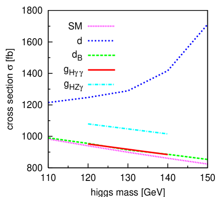
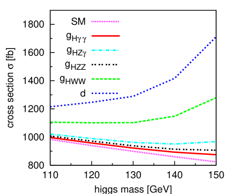
Figure 2: Production cross section of a Higgs Boson with anomalous couplings in addition to the SM $HVV$ interactions. Left: The upper bounds for $g_{H\gamma\gamma}$ and $g_{HZ\gamma}^{(2)}$ given in Table 1 and the upper 95% CL bounds for $d$ and $d_{B}$, given by the L3 collaboration, are used. Right: The upper bound for $d$ is used for the different couplings.

On the one hand Fig. 2 shows the LHC production cross section for a Higgs boson with only a single additional anomalous coupling of Eq. (2.4) and on the other hand production cross sections for the parameters $d$ or $d_{B}$ are shown. On the left side, couplings $g_{H\gamma\gamma}$ and $g_{HZ\gamma}^{(2)}$ have been used which saturate the 95% CL bounds of Table 1. $g_{H\gamma\gamma}$ is already tightly constrained by the absence of an $e^{+}e^{-}\to H\gamma,\;H\to\gamma\gamma$ signal at LEP. Only minor deviations from the SM are allowed in the VBF Higgs production cross section due to this coupling alone. The direct limit on a pure $g_{HZ\gamma}^{(2)}$ coupling is weaker, since the more difficult $H\to Z\gamma$ partial width would have been enhanced at LEP, and this coupling still allows for significant deviations from SM expectations in the Higgs production cross section at the LHC. The parameter $d_{B}$ only leads to small deviations from the SM and can be neglected, whereas a large enhancement due to the parameter $d$ is still possible.

On the right hand side of Fig. 2 the indirectly determined constraints on the anomalous couplings of Table 2 and, thus, for $d_{B}=0$ have been used and cross sections for individual anomalous couplings at the 95% CL limit are shown. $g_{HZ\gamma}^{(2)}$ and $g_{HZZ}^{(2)}$ already have strong bounds and do not lead to significant deviations from the SM. However, $g_{HWW}^{(2)}$ as given in Eq. (2.6) only depends on $d$ and is mainly responsible for the large enhancement of the cross section.

In Higgs decay, the effects of $g_{H\gamma\gamma}$ and $g_{HZ\gamma}^{(2)}$ are the most important ones, because the $H\gamma\gamma$ and $HZ\gamma$ couplings in the SM only appear at one loop level and are therefore very small. With the anomalous couplings the partial decay widths of $H\to\gamma\gamma,Z\gamma$ can be enhanced by several orders of magnitude and even become the dominant decay channels. Since in the SM the couplings of the Higgs boson to $W$ and $Z$ bosons appear already at tree level, the effects of anomalies in the $HZZ$ and $HWW$ couplings are not so strong.

  

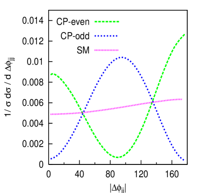
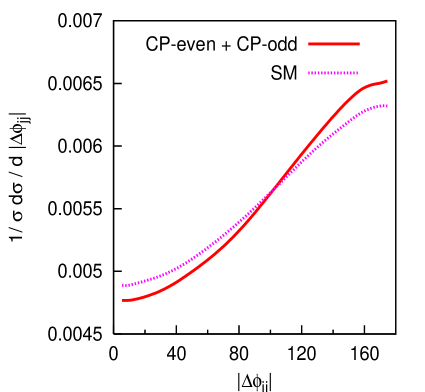
Figure 3: Normalized azimuthal angle correlations of the two tagging jets in VBF as in Ref. [4] for a Higgs mass of 120 GeV and $d$ = 0.18 or, respectively, $\tilde{d}$ = 0.18. Left: Purely CP-even, CP-odd or SM couplings. Right: CP-even and CP-odd couplings of the same size.

In order to determine the tensor structure of the $HVV$ couplings, for any scalar particle $H$ found at the LHC, the distributions of the two tagging jets are an important tool. However, most distributions, like the jet transverse momentum, jet energy or dijet invariant mass, may depend strongly on the form factors and, therefore, are hard to predict without specifying the underlying model of new physics. An exception is the azimuthal angle between the two tagging jets in the final state. The shape of $d\sigma/d|\Delta\phi_{jj}|$ is quite insensitive to form factor effects [8] and it provides for an excellent distinction between the three tensor structures of Eq. (1.1). The characteristic distributions are shown in Fig. 3. For a purely CP-odd coupling the cross section is suppressed at 0 and 180 degrees, for a CP-even coupling this dip appears at 90 degrees, while a pure SM coupling produces a rather flat $|\Delta\phi_{jj}|$ distribution [4]. Unfortunately, when both CP-even and CP-odd couplings of similar strength are present, the dips cancel and result in a distribution which is very similar to SM expectations.

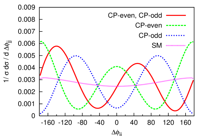
Figure 4: Normalized distribution of the azimuthal angle $\Delta\phi_{jj}$ defined in Eq. (4.2) for a Higgs mass of 120 GeV and a mixed CP scenario ($d$ = $\tilde{d}$ = 0.18, red solid curve), a CP-even anomalous coupling ($d$ = 0.18, $\tilde{d}$ = 0, green dashed curve), a CP-odd coupling ($d$ = 0, $\tilde{d}$ = 0.18, blue dotted curve) and the SM case (purple narrow dotted line).

The missing information is contained in the sign of the azimuthal angle between the tagging jets. Naively one might assume that this sign cannot be defined unambiguously in $pp$ collisions because an azimuthal angle switches sign when viewed along the opposite beam direction. However, in doing so, the “toward” and the “away” tagging jets also switch place, i.e. one should take into account the correlation of the tagging jets with the two distinct beam directions. Defining $\Delta\phi_{jj}$ as the azimuthal angle of the “away” jet minus the azimuthal angle of the “toward” jet, a switch of the two beam directions leaves the sign of $\Delta\phi_{jj}$ intact. In order to be precise, let us define the normalized four-momenta of the two proton beams as $b_{+}$ and $b_{-}$, while $p_{+}$ and $p_{-}$ denote the four-momenta of the two tagging jets, where ${\bf p_{+}}$ points into the same detector hemisphere as ${\bf b_{+}}$. Then

$$\varepsilon_{\mu\nu\rho\sigma}b_{+}^{\mu}p_{+}^{\nu}b_{-}^{\rho}p_{-}^{\sigma}=2p_{T,+}p_{T,-}\sin(\phi_{+}-\phi_{-})=2p_{T,+}p_{T,-}\sin\Delta\phi_{jj}$$ (4.2)

provides the sign of $\Delta\phi_{jj}$. This definition is manifestly invariant under the interchange $(b_{+},p_{+})\leftrightarrow(b_{-},p_{-})$ and we also note that $\Delta\phi_{jj}$ is a parity odd observable.

  

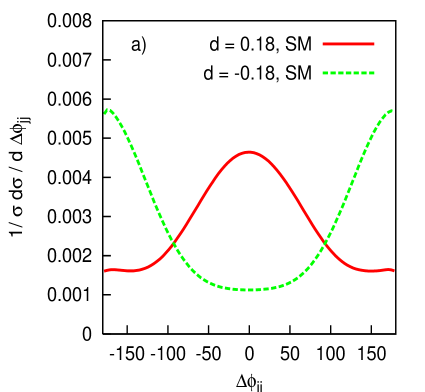
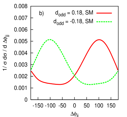
Figure 5: Normalized distribution of the azimuthal angle for a Higgs mass of 120 GeV for SM and anomalous couplings (a) $d=\pm 0.18$ and (b) $\tilde{d}=\pm 0.18$. The new definition of the azimuthal angle is used.

The corresponding azimuthal angle distribution is shown in Fig. 4 for three scenarios of purely anomalous couplings (i.e. no SM contribution, $a_{1}(q_{1},q_{2})=0$) and for the SM case. The characteristic dips for purely CP-even and CP-odd couplings are still present and occur at $\pm$90 degrees and $0,\pm 180$ degrees, respectively. In the case of mixed CP-even and CP-odd couplings,

$$d=d_{0}\;\sin\alpha\;,\qquad\tilde{d}=d_{0}\;\cos\alpha\;,$$ (4.3)

and no SM contribution, the positions of the dips shift to $\Delta\phi_{jj}=-\alpha$ and $\Delta\phi_{jj}=-\alpha+\pi$ (modulo $2\pi$). This shift also explains why $|\Delta\phi_{jj}|$ loses information in the mixed CP case: when folding over the $\Delta\phi_{jj}$-distribution at $\Delta\phi_{jj}=0$, the positions of the dips do not match and, hence, they fill up.

A more complicated picture emerges when considering interference effects between a SM contribution and anomalous couplings, i.e. when $a_{1}$ and one or two of the anomalous form factors $a_{i}(q_{1},q_{2}),\;(i=2,3)$ of Eq. (1.1) are present simultaneously. For the sake of the argument, let us assume that $a_{1}$ has SM strength and that $a_{2}$ and $a_{3}$ are real. The full amplitude can then be written as

$$M=M_{SM}+a_{2}M_{CP-even}+a_{3}M_{CP-odd}$$ (4.4)

which results in the matrix element squared:

$$|M|^{2} = |M_{SM}|^{2}+a_{2}^{2}|M_{CP-even}|^{2}+a_{3}^{2}|M_{CP-odd}|^{2}$$ (4.5)

$$+\underbrace{a_{2}2Re\left(M_{SM}^{*}M_{CP-even}\right)+a_{3}2Re\left((M_{SM}+a_{2}M_{CP-even})^{*}M_{CP-odd}\right)}_{\mathrm{Interference}\ \mathrm{term}}$$

For smallish anomalous couplings $a_{2}$ and/or $a_{3}$ the interference terms provide the best sensitivity to new physics effects and these interference terms also reveal the sign of anomalous couplings.

When integrating over phase space, the three contributions $M_{SM}$, $M_{CP-even}$ and $M_{CP-odd}$ may change relative signs and, thus, interference effects may cancel. For the $|\Delta\phi_{jj}|$ distribution this is indeed a problem: $M_{SM}$ and $M_{CP-even}$ are even functions of $\Delta\phi_{jj}$ while $M_{CP-odd}$ is odd in $\Delta\phi_{jj}$. This means that the interference proportional to $a_{3}$ integrates to zero when the sign of $\Delta\phi_{jj}$ is not measured. The $a_{2}$ interference term, on the other hand, does not suffer from this problem and can be observed in $d\sigma/d|\Delta\phi_{jj}|$ already [4]: the shape of the distribution changes dramatically when flipping the sign of the anomalous coupling.

The problem for the $a_{3}$ interference term is resolved by taking into account the parity odd nature of the term linear in $M_{CP-odd}$, namely by plotting $d\sigma/d\Delta\phi_{jj}$. The effect is demonstrated in Fig. 5 where the interference of the SM amplitude with a purely CP-even or purely CP-odd anomalous coupling is shown for the two signs of the anomalous couplings. For the CP-even coupling the interference term is even in $\Delta\phi_{jj}$ and, hence, is fully present when plotting the absolute value of $\Delta\phi_{jj}$. For a CP-odd anomalous coupling the interference is odd in $\Delta\phi_{jj}$ and completely disappears in $d\sigma/d|\Delta\phi_{jj}|$.

As noted above, $\Delta\phi_{jj}$ is a parity odd observable. Finding a $\Delta\phi_{jj}$ asymmetry as in Fig. 5(b) would show that parity is violated in the process $qq\to qqH$. Since the SM distribution (at tree level) is $\Delta\phi_{jj}$-even, the parity violation must originate from a parity-odd coupling, namely $a_{3}$ in the $HVV$ vertex. This term is also CP-odd. Such a coupling, occurring at the same time as the CP-even SM amplitude or the CP-even coupling $a_{2}$, implies CP-violation in the Higgs sector. In this sense, the observation of an asymmetry in the $\Delta\phi_{jj}$ distribution would directly demonstrate CP-violation in the Higgs sector.

5 Conclusions

With VBFNLO we have available a parton level Monte Carlo program which allows to calculate Higgs production via vector boson fusion, including NLO QCD corrections. The program has now been extended to support anomalous $HVV$ couplings in both the production and the Higgs decay process.

For Higgs masses below about 160 GeV, the non-observation of $H\gamma$ signals at LEP puts stringent constraints on anomalous $HVV$ couplings. We have analyzed the size of deviations in VBF Higgs signals due to anomalous couplings which are allowed by the LEP data. Within these bounds, anomalous HWW couplings can enhance the production cross section of a Higgs boson in VBF at the LHC by more than 10% whereas effects from anomalous $H\gamma\gamma$ couplings are negligible and the effects of anomalous $HZ\gamma$ and $HZZ$ couplings are also small. In contrast, the relevant anomalous couplings in Higgs decay are H$\gamma\gamma$ and HZ$\gamma$. Even with the existing bounds from LEP those couplings can enhance partial Higgs decay widths by several orders of magnitude and, therefore, lead to measurable effects in Higgs signals at the LHC.

A sensitive probe of anomalous Higgs couplings in the production process is the azimuthal angle between the tagging jets, as defined in Eq. (4.2). The azimuthal angle distribution is largely form factor independent and allows to extract the complete information about the tensor structure of the $HVV$ coupling. An odd contribution to the $\Delta\phi_{jj}$ distribution proves the presence of parity violation in Higgs production and signals CP-violation in the Higgs sector.

The $\Delta\phi_{jj}$ distribution should be analyzed for all $Hjj$ production processes at the LHC, in particular also for gluon fusion. Since heavy fermion loops give rise to effective $Hgg$ vertices with the tensor structures given by the $a_{2}$ and $a_{3}$ terms in Eq. (1.1), the same qualitative behavior of $d\sigma/d\Delta\phi_{jj}$ arises in gluon fusion events also and distinguishes scalar and pseudo-scalar Higgs couplings to heavy fermions [22] and also signals mixed scalar and pseudo-scalar couplings, i.e. CP violating effects in the Higgs sector. We will analyze these effects in a future publication [23].

References

- [1] M. Spira, Fortsch. Phys. 46 (1998) 203 [arXiv:hep-ph/9705337].
- [2] For a recent review, see A. Djouadi, arXiv:hep-ph/0503172.
- [3] D. Zeppenfeld, R. Kinnunen, A. Nikitenko and E. Richter-Was, Phys. Rev. D 62 (2000) 013009 [arXiv:hep-ph/0002036]; A. Belyaev and L. Reina, JHEP 0208, 041 (2002) [arXiv:hep-ph/0205270]; M. Dührssen et al., Phys. Rev. D 70 (2004) 113009 [arXiv:hep-ph/0406323].
- [4] T. Plehn, D. L. Rainwater and D. Zeppenfeld, Phys. Rev. Lett. 88 (2002) 051801 [arXiv:hep-ph/0105325].
- [5] T. Han, G. Valencia and S. Willenbrock, Phys. Rev. Lett. 69, 3274 (1992) [arXiv:hep-ph/9206246].
- [6] T. Figy, C. Oleari and D. Zeppenfeld, Phys. Rev. D 68, 073005 (2003) [arXiv:hep-ph/0306109].
- [7] E. L. Berger and J. Campbell, Phys. Rev. D 70 (2004) 073011 [arXiv:hep-ph/0403194].
- [8] T. Figy and D. Zeppenfeld, Phys. Lett. B 591, 297 (2004) [arXiv:hep-ph/0403297].
- [9] C. Oleari and D. Zeppenfeld, Phys. Rev. D 69 (2004) 093004 [arXiv:hep-ph/0310156]; B. Jager, C. Oleari and D. Zeppenfeld, JHEP, in press [arXiv:hep-ph/0603177]; B. Jager, C. Oleari and D. Zeppenfeld, Phys. Rev. D 73 (2006) 113006 [arXiv:hep-ph/0604200].
- [10] W. Buchmüller and D. Wyler, Nucl. Phys. B 268 (1986) 621.
- [11] K. Hagiwara, S. Ishihara, R. Szalapski and D. Zeppenfeld, Phys. Rev. D 48 (1993) 2182.
- [12] K. Hagiwara, R. Szalapski and D. Zeppenfeld, Phys. Lett. B 318 (1993) 155 [arXiv:hep-ph/9308347].
- [13] O. J. P. Eboli, M. C. Gonzalez-Garcia, S. M. Lietti and S. F. Novaes, Phys. Lett. B 478 (2000) 199 [arXiv:hep-ph/0001030].
- [14] A. V. Manohar and M. B. Wise, Phys. Lett. B 636 (2006) 107 [arXiv:hep-ph/0601212].
- [15] J. Erler and P. Langacker, Phys. Lett. B 592 (2004) 1 [arXiv:hep-ph/0407097].
- [16] P. Achard et al. [L3 Collaboration], Phys. Lett. B 589 (2004) 89 [arXiv:hep-ex/0403037].
- [17] K. Hagiwara, R. D. Peccei, D. Zeppenfeld and K. Hikasa, Nucl. Phys. B 282 (1987) 253.
- [18] [LEP Collaborations], arXiv:hep-ex/0412015.
- [19] S. Schael et al. [ALEPH Collaboration], Phys. Lett. B 614 (2005) 7.
- [20] N. Kauer, T. Plehn, D. L. Rainwater and D. Zeppenfeld, Phys. Lett. B 503 (2001) 113 [arXiv:hep-ph/0012351].
- [21] E. Boos et al., arXiv:hep-ph/0109068.
- [22] V. Hankele, G. Klämke and D. Zeppenfeld, arXiv:hep-ph/0605117.
- [23] G. Klämke and D. Zeppenfeld, in preparation.