Azimuthal Dependence of the Heavy Quark Initiated Contributions to DIS

Abstract

We analyze the azimuthal dependence of the heavy-quark-initiated contributions to the lepton-nucleon deep inelastic scattering (DIS). First we derive the relations between the parton level semi-inclusive structure functions and the helicity $\gamma^{*}Q$ cross sections in the case of arbitrary values of the heavy quark mass. Then the azimuth-dependent ${\cal O}(\alpha_{s})$ lepton-quark DIS is calculated in the helicity basis. Finally, we investigate numerically the properties of the $\cos\varphi$ and $\cos 2\varphi$ distributions caused by the photon-quark scattering (QS) contribution. It turns out that, contrary to the basic photon-gluon fusion (GF) component, the QS mechanism is practically $\cos 2\varphi$-independent. This fact implies that measurements of the azimuthal distributions in charm leptoproduction could directly probe the charm density in the proton.

I Introduction

The notion of the intrinsic charm (IC) content of the proton has been introduced over 25 years ago in Refs BHPS ; BPS . It was shown that, in the light-cone Fock space picture brod1 ; brod2 , it is natural to expect a five-quark state contribution, $\left|uudc\bar{c}\right\rangle$, to the proton wave function. This component can be generated by $gg\rightarrow c\bar{c}$ fluctuations inside the proton where the gluons are coupled to different valence quarks. The original concept of the charm density in the proton BHPS ; BPS has nonperturbative nature since a five-quark contribution $\left|uudc\bar{c}\right\rangle$ scales as $1/m^{2}$ where $m$ is the $c$-quark mass polyakov .

A decade ago another point of view on the charm content of the proton has been proposed in the framework of the variable flavor number scheme (VFNS) ACOT ; collins . Within the VFNS, the mass logarithms of the type $\alpha_{s}\ln\left(Q^{2}/m^{2}\right)$ are resummed through the all orders into a heavy quark density which evolves with $Q^{2}$ according to the standard DGLAP evolution equation. Hence this approach introduces the parton distribution functions (PDFs) for the heavy quarks and changes the number of active flavors by one unit when a heavy quark threshold is crossed. Note also that the charm density arises within the VFNS perturbatively via the $g\rightarrow c\bar{c}$ evolution. Some recent developments concerning the VFNS are presented in Refs. Thorne-NNLO ; CTEQ6-5HQ ; CTEQ6HQ ; chi ; SACOT .

Presently, both nonperturbative IC and perturbative charm density are widely used for a phenomenological description of available data. (A recent review of the theory and experimental constraints on the charm quark distribution can be found in Refs. pumplin ; brod-higgs ). In particular, practically all the recent versions of the CTEQ CTEQ6 and MRST MRST2004 sets of PDFs are based on the VFN schemes and contain a charm density. At the same time, the key question remains open: How to measure the charm content of the proton? The basic theoretical problem is that radiative corrections to the leading order (LO) predictions for the heavy quark production cross sections are large: they increase the Born level results by approximately a factor of two at energies of the fixed target experiments. On the other hand, perturbative instability leads to a high sensitivity of the theoretical calculations to standard uncertainties in the input QCD parameters: $m$, $\mu_{R}$, $\mu_{F}$, $\Lambda_{QCD}$ and PDFs. For this reason, one can only estimate the order of magnitude of the pQCD predictions for the heavy flavor production cross sections Mangano-N-R ; Frixione-M-N-R .

At not very high energies, the main reason for large NLO cross sections of heavy flavor production in $\gamma g$ Ellis-Nason ; Smith-Neerven , $\gamma^{*}g$ LRSN , and $gg$ Nason-D-E-1 ; Nason-D-E-2 ; Nason-D-E-3 ; BKNS collisions is the so-called threshold (or soft-gluon) enhancement. This strong logarithmic enhancement has universal nature in the perturbation theory since it originates from incomplete cancellation of the soft and collinear singularities between the loop and the bremsstrahlung contributions. Large leading and next-to-leading threshold logarithms can be resummed to all orders of perturbative expansion using the appropriate evolution equations Contopanagos-L-S ; Laenen-O-S ; Kidonakis-O-S . Soft gluon resummation of the threshold Sudakov logarithms indicates that the higher-order contributions to the heavy flavor production are also sizeable. (For a review see Refs. Laenen-Moch ; kid2 ; kid1 ).

Since production cross sections are not perturbatively stable, it is of special interest to study those observables that are well-defined in pQCD. A nontrivial example of such an observable was proposed in Refs. we1 ; we2 ; we4 ; we3 where the azimuthal $\cos 2\varphi$ asymmetry in heavy quark photo- and leptoproduction has been analyzed . In particular, the Born level results have been considered we1 ; we4 and the NLO soft-gluon corrections to the basic mechanism, photon-gluon fusion (GF), have been calculated we2 ; we4 . It was shown that, contrary to the production cross sections, the $\cos 2\varphi$ asymmetry in heavy flavor photo- and leptoproduction is quantitatively well defined in pQCD: the contribution of the dominant GF mechanism to the asymmetry is stable, both parametrically and perturbatively. This fact provides the motivation for investigation of the photon-(heavy) quark scattering (QS) contribution to the $\varphi$-dependent lepton-hadron deep inelastic scattering (DIS).

In the present paper, we calculate the azimuthal dependence of the next-to-leading order (NLO) ${\cal O}(\alpha_{em}\alpha_{s})$ heavy-flavor-initiated contributions to DIS. To our knowledge, pQCD predictions for the $\varphi$-dependent $\gamma^{*}Q$ cross sections in the case of arbitrary values of the heavy quark mass $m$ and $Q^{2}$ are not available in the literature. Moreover, there is a confusion among the existing results for azimuth-independent $\gamma^{*}Q$ cross sections.

The NLO corrections to the $\varphi$-independent lepton-quark DIS have been calculated (for the first time) a long time ago in Ref. HM , and have been re-calculated recently in KS . The authors of Ref. KS conclude that there are errors in the NLO expression for $\sigma^{(2)}$ given in Ref. HM . We disagree with this conclusion. It will be shown below that a correct interpretation of the notations for the production cross sections used in HM leads to a complete agreement between the results presented in Refs. HM , KS and present paper.

As to the $\varphi$-dependent $\gamma^{*}Q$ cross sections, our main result can be formulated as follows. Contrary to the basic GF component, the QS mechanism is practically $\cos 2\varphi$-independent. This is due to the fact that the QS contribution to the $\cos 2\varphi$ asymmetry is absent (for the kinematic reason) at LO and is negligibly small (of the order of $1\%$) at NLO. This fact indicates that the azimuthal distributions in charm leptoproduction could be a good probe of the charm density in the proton. In detail, the possibility of measuring the charm content of the proton using the $\cos 2\varphi$ asymmetry will be investigated in a forthcoming publication we5 .

Concerning the experimental aspects, azimuthal asymmetries in charm leptoproduction can, in principle, be measured in the COMPASS experiment at CERN, as well as in future studies at the proposed eRHIC eRHIC ; EIC and LHeC LHeC colliders at BNL and CERN, correspondingly.

The outline of this paper is as follows. In Section II, we derive the relations between the parton level semi-inclusive structure functions and the helicity $\gamma^{*}Q$ cross sections in the case of arbitrary values of the heavy quark mass. As explained in Ref. AOT , in the presence of non-zero masses, it is the helicity basis that provides the simplest connections between the hadron- and parton-level production cross sections. In Section III, we present the NLO ${\cal O}(\alpha_{em}\alpha_{s})$ predictions for the $\varphi$-dependent lepton-quark DIS in the helicity basis. Our calculations are compared with available results in Section IV. In Section V, a numerical investigation of the $\cos\varphi$ and $\cos 2\varphi$ distributions caused by the QS contribution is given. In particular, we provide a simple parton level proof of the fact that the QS mechanism is practically $\cos 2\varphi$-independent. Our conclusions are presented in Section VI.

II Azimuth-Dependent Structure Functions in the Helicity Basis

In this Section, the helicity formalism for the semi-inclusive $\gamma^{*}Q$ cross sections in the case of arbitrary values of the heavy quark mass is presented. This is a purely kinematical analysis, which will set the notation to be used later on. In fact, we extend the helicity approach proposed in Ref. AOT to the case of $\varphi$-dependent leptoproduction using the method formulated in Ref. dombey .

We consider the semi-inclusive deep inelastic lepton-quark scattering. The momentum assignment will be denoted as

$$l(\ell)+Q(k)\rightarrow l^{\prime}(\ell-q)+Q^{\prime}(p)+X(p_{X}).$$ (1)

The following definition of partonic kinematic variables is used:

$$y=\frac{q\cdot k}{\ell\cdot k},\qquad\qquad z=\frac{Q^{2}}{2q\cdot k},\qquad\qquad\lambda=\frac{m^{2}}{Q^{2}},\qquad\qquad Q^{2}=-q^{2}.$$ (2)

The differential cross section of the reaction (1), d${}^{3}\hat{\sigma}_{lQ}$, is defined in terms of the quark tensor $\widetilde{W}_{Q}^{\mu\nu}$:

$$\ell_{0}^{\prime}\frac{\text{d}^{3}\hat{\sigma}_{lQ}}{\text{d}^{3}\ell^{\prime}}=2\frac{\text{d}^{3}\hat{\sigma}_{lQ}}{\text{d}y\text{d}Q^{2}\text{d}\varphi}=\frac{2z}{y}\frac{\text{d}^{3}\hat{\sigma}_{lQ}}{\text{d}z\text{d}Q^{2}\text{d}\varphi}=\frac{\alpha_{em}^{2}}{(\ell\cdot k)Q^{4}}L_{\mu\nu}\widetilde{W}_{Q}^{\mu\nu}\frac{\text{d}^{3}p}{(2\pi)^{3}2p_{0}},$$ (3)

where $\ell^{\prime}_{\mu}=(\ell-q)_{\mu}$ is the 4-momentum of the final lepton. In the target rest frame, the azimuth $\varphi$ is the angle between the lepton scattering plane and the heavy quark production plane, defined by the exchanged photon and the detected quark $Q^{\prime}$ (see Fig. 1). The covariant definition of $\varphi$ is

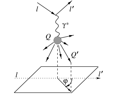
Figure 1: Definition of the azimuthal angle $\varphi$ in the target rest frame.

$$\cos\varphi = \frac{r\cdot n}{\sqrt{-r^{2}}\sqrt{-n^{2}}},\qquad\qquad\qquad\qquad\sin\varphi=\frac{Q^{2}\sqrt{1+4\lambda z^{2}}}{2z\sqrt{-r^{2}}\sqrt{-n^{2}}}~{}n\cdot\ell,$$

$$r^{\mu} = \varepsilon^{\mu\nu\alpha\beta}k_{\nu}q_{\alpha}\ell_{\beta},\qquad\qquad\qquad\qquad\quad n^{\mu}=\varepsilon^{\mu\nu\alpha\beta}q_{\nu}k_{\alpha}p_{\beta}.$$ (4)

The explicit expression for the lepton tensor $L_{\mu\nu}$ is:

$$L_{\mu\nu}=\mathop{\overline{\sum}}\limits_{\text{spin}}\left\langle\ell\left|j_{\nu}^{\dagger}\right|\ell^{\prime}\right\rangle\left\langle\ell^{\prime}\left|j_{\mu}\right|\ell\right\rangle=2\ell_{\mu}\ell_{\nu}^{\prime}+2\ell_{\nu}\ell_{\mu}^{\prime}-Q^{2}g_{\mu\nu},$$ (5)

where $\mathop{\overline{\sum}}\limits_{\text{spin}}$denotes a sum over all final helicity states and an averaging over all initial spin variables. The semi-inclusive quark tensor $\widetilde{W}_{Q}^{\mu\nu}$ is defined as follows:

$$\widetilde{W}_{Q}^{\mu\nu}(q,k,p)=\frac{1}{4\pi}\mathop{\overline{\sum}}\limits_{X(p_{X}),\text{spin}}\left\langle k\left|J^{\mu}\right|p,p_{X}\right\rangle\left(2\pi\right)^{4}\delta^{(4)}\left(q+k-p-p_{X}\right)\left\langle p_{X},p\left|J^{\dagger\nu}\right|k\right\rangle,$$ (6)

where sums and integrals over all the unobserved final states $X$ of momentum $p_{X}^{\mu}$ are implied.

To construct the parton tensor describing the semi-inclusive $\gamma^{*}Q$ DIS, it is convenient to introduce two 4-vectors:

$$v^{\mu}=\frac{\varepsilon_{\tau\nu\alpha\beta}\varepsilon^{\tau\gamma\theta\mu}q^{\nu}k^{\alpha}p^{\beta}k_{\gamma}q_{\theta}}{(q\cdot k)\sqrt{-n^{2}}\sqrt{1+4\lambda z^{2}}},\qquad\qquad\qquad\qquad\qquad\qquad w^{\mu}=k^{\mu}+\frac{q\cdot k}{Q^{2}}q^{\mu},$$ (7)

that obey the following conditions: $v\cdot k=v\cdot q=0,$ $v^{2}=-1$ and $w\cdot q=0,$ $w\cdot k=w^{2}=m^{2}\left(1+4\lambda z^{2}\right)/4\lambda z^{2}$. In terms of $v^{\mu}$ and $w^{\nu}$, $\widetilde{W}_{Q}^{\mu\nu}$ has the following structure:

$$\widetilde{W}_{Q}^{\mu\nu}(q,k,p)=-\left(g^{\mu\nu}-\frac{q^{\mu}q\nu}{q^{2}}\right)\widetilde{W}_{1}+\frac{w^{\mu}w^{\nu}}{m^{2}}\widetilde{W}_{2}+\left(w^{\mu}v^{\nu}+w^{\nu}v^{\mu}\right)\frac{\widetilde{W}_{I}}{m}+v^{\mu}v^{\nu}\widetilde{W}_{A},$$ (8)

that obeys all the necessary conservation laws. In particular, $\widetilde{W}_{Q}^{\mu\nu}q_{\mu}=0$. The scalar coefficients $\widetilde{W}_{i}$ $(i=1,2,I,A)$ are the semi-inclusive parton-level structure functions for the process (1), $\widetilde{W}_{i}\equiv\widetilde{W}_{i}\left(z,\lambda,p_{X}^{2},q\cdot p\right)$.

For parton-model considerations, is it convenient to use the so-called colliner frames where the 3-momenta of the virtual photon and initial quark are antiparallel to each other, $\vec{q}\parallel(-\vec{k})$. Evidently, an arbitrary colliner frame can be obtained from the initial quark rest system with the help of a Lorentz boost along $\vec{q}$. Pointing the $z$-axis along $\vec{q}$, we will have in a colliner frame:

$$v^{\mu} = (0,\vec{v}_{\perp},0),\qquad\qquad\qquad\qquad\qquad\qquad\vec{v}_{\perp}=\frac{\vec{p}_{\perp}}{\left|\vec{p}_{\perp}\right|},$$ (9)

$$w^{\mu} = \frac{Q\sqrt{1+4\lambda z^{2}}}{2\sqrt{z}}e_{0}^{\mu},\qquad\qquad\quad\qquad\qquad\;\,e_{0}^{\mu}=\frac{1}{Q}(\left|\vec{q}\right|,\vec{0}_{\perp},q_{0}),$$ (10)

where $Q=\sqrt{-q^{2}}$ and $e_{0}^{\mu}$ describes the longitudinal polarization of the virtual photon, $\gamma^{*}$. It is also useful to define the scalar, $e_{q}^{\mu}$, and transverse, $e_{\pm}^{\mu}$, polarization vectors:

$$e_{q}^{\mu}=\frac{q^{\mu}}{Q},\qquad\qquad\qquad\qquad\qquad\qquad\qquad e_{\pm}^{\mu}=\frac{1}{\sqrt{2}}\left(0,\mp 1,-i,0\right).$$ (11)

Note the completeness relation

$$e_{+}^{\mu}e_{+}^{\nu*}+e_{-}^{\mu}e_{-}^{\nu*}-e_{0}^{\mu}e_{0}^{\nu*}+e_{q}^{\mu}e_{q}^{\nu*}=-g^{\mu\nu},$$ (12)

and the normalization for the physical states:

$$e_{r}\cdot e_{s}^{*}=(-1)^{s}\delta_{rs},\qquad\qquad\qquad(r,s=0,\pm 1).$$ (13)

One can see from Eqs. (9,10) that it is merely the scalar coefficient functions $\widetilde{W}_{i}$ $(i=1,2,I,A)$ depend on the final quark momentum $p$ in a collinear frame. For this reason, we can integrate the semi-inclusive quark tensor $\widetilde{W}_{Q}^{\mu\nu}(q,k,p)$ over $\vec{p}$ and obtain the inclisive quantity $W_{Q}^{\mu\nu}(q,k)$:

$$W_{Q}^{\mu\nu}(q,k) = \int\frac{\text{d}^{3}p}{(2\pi)^{3}2p_{0}}\widetilde{W}_{Q}^{\mu\nu}(q,k,p)$$

$$= -\left(g^{\mu\nu}-\frac{q^{\mu}q\nu}{q^{2}}\right)\left(\hat{W}_{1}-\frac{1}{2}\hat{W}_{A}\right)+\frac{w^{\mu}w^{\nu}}{m^{2}}\left(\hat{W}_{2}-\frac{2\lambda z^{2}}{1+4\lambda z^{2}}\hat{W}_{A}\right)+\left(w^{\mu}v^{\nu}+w^{\nu}v^{\mu}\right)\frac{\hat{W}_{I}}{m}+v^{\mu}v^{\nu}\hat{W}_{A}.$$

The inclusive coefficient functions $W_{i}(z,\lambda)$ $\ (i=1,2,I,A)$ are related to the semi-inclusive ones as follows:

$$\hat{W}_{1}(z,\lambda) = \int\frac{\text{d}^{3}p}{(2\pi)^{3}2p_{0}}\left(\widetilde{W}_{1}+\frac{1}{2}\widetilde{W}_{A}\right)\left(z,\lambda,p_{X}^{2},q\cdot p\right),\qquad\qquad\;\hat{W}_{I}(z,\lambda)=\int\frac{\text{d}^{3}p}{(2\pi)^{3}2p_{0}}\widetilde{W}_{I}\left(z,\lambda,p_{X}^{2},q\cdot p\right),$$ (15)

$$\hat{W}_{2}(z,\lambda) = \int\frac{\text{d}^{3}p}{(2\pi)^{3}2p_{0}}\left(\widetilde{W}_{2}+\frac{2\lambda z^{2}}{1+4\lambda z^{2}}\widetilde{W}_{A}\right)\left(z,\lambda,p_{X}^{2},q\cdot p\right),\quad\!\hat{W}_{A}(z,\lambda)=\int\frac{\text{d}^{3}p}{(2\pi)^{3}2p_{0}}\widetilde{W}_{A}\left(z,\lambda,p_{X}^{2},q\cdot p\right).$$

Integrating $W_{Q}^{\mu\nu}(q,k)$ over the lepton azimuth $\varphi$ defined by Eqs. (4), one can reproduce the well-known expression for totally inclusive DIS:

$$\frac{1}{2\pi}\int\limits_{0}^{2\pi}\text{d}\varphi W_{Q}^{\mu\nu}(q,k)=-\left(g^{\mu\nu}-\frac{q^{\mu}q\nu}{q^{2}}\right)\hat{W}_{1}(z,Q^{2})+\frac{w^{\mu}w^{\nu}}{m^{2}}\hat{W}_{2}(z,Q^{2}).$$ (16)

Note that the above relation can easily be obtained from Eq. (II) taking into account that $\int_{0}^{2\pi}$d$\varphi\,v^{\mu}v^{\nu}=\pi\left(e_{+}^{\mu}e_{+}^{\nu*}+e_{-}^{\mu}e_{-}^{\nu*}\right)=\pi\left(-g^{\mu\nu}+e_{0}^{\mu}e_{0}^{\nu*}-e_{q}^{\mu}e_{q}^{\nu*}\right).$

Now the cross section for the inclusive azimuth-dependent lepton-quark DIS can be written as

$$\frac{\text{d}^{3}\hat{\sigma}_{lQ}}{\text{d}z\text{d}Q^{2}\text{d}\varphi}=\frac{y}{z}\frac{\text{d}^{3}\hat{\sigma}_{lQ}}{\text{d}y\text{d}Q^{2}\text{d }\varphi}=\frac{y}{Q^{2}}\frac{\text{d}^{3}\hat{\sigma}_{lQ}}{\text{d}z\text{d}y\text{d}\varphi}=\frac{\alpha_{em}^{2}y^{2}}{Q^{6}}L_{\mu\nu}W_{Q}^{\mu\nu}.$$ (17)

To derive the relations between the invariant and helicity structure functions, we use the completeness (12) which implies that

$$L_{\mu\nu}W_{Q}^{\mu\nu}=\sum\limits_{r,s}\rho_{rs}\hat{F}_{rs},$$ (18)

where the quark and lepton helicity structure functions ($\hat{F}_{rs}$ and $\rho_{rs}$, respectively) are defined as

$$\hat{F}_{rs}=e_{r}^{\mu}W_{Q,\mu\nu}e_{s}^{\nu*},\qquad\qquad\quad\ \ \qquad\qquad\ \rho_{rs}=(-1)^{r+s}e_{r}^{\mu*}L_{\mu\nu}e_{s}^{\nu}.$$ (19)

Choosing the $x$-axis along $\vec{v}_{\perp}$ defined by Eq. (9), we obtain for the quark helicity structure functions $\hat{F}_{rs}(z,\lambda)$:

$$\hat{F}_{{+}{+}} = \hat{F}_{{-}{-}}=\hat{W}_{1},\qquad\qquad\quad\ \ \ \qquad\qquad\quad\quad\;\;\ \ \ \qquad\qquad\quad\ \ \ \ \hat{F}_{\mathop{0}\mathop{0}}=-\hat{W}_{1}+\frac{1+4\lambda z^{2}}{4\lambda z^{2}}\hat{W}_{2},$$

$$\hat{F}_{{+}\mathop{0}} = \hat{F}_{\mathop{0}{+}}=-\hat{F}_{{-}\mathop{0}}=-\hat{F}_{\mathop{0}{-}}=\frac{1}{2}\sqrt{\frac{1+4\lambda z^{2}}{2\lambda z^{2}}}\hat{W}_{I},\qquad\qquad\qquad\,\hat{F}_{{+-}}=\hat{F}_{{-+}}=-\frac{1}{2}\hat{W}_{A}.$$ (20)

The lepton tensor $\rho_{rs}\left(\hat{\varepsilon},\varphi\right)$ has the following form in the helicity basis:

$$\rho_{{++}} = \rho_{{--}}=\frac{Q^{2}}{1-\hat{\varepsilon}},\qquad\qquad\quad\ \ \ \qquad\qquad\quad\ \ \ \qquad\qquad\quad\ \ \ \ \ \ \,\rho_{\mathop{0}\mathop{0}}=\frac{2Q^{2}\hat{\varepsilon}}{1-\hat{\varepsilon}},$$ (21)

$$\rho_{{+}\mathop{0}} = \rho_{\mathop{0}{+}}^{*}=-\rho_{{-}\mathop{0}}^{*}=-\rho_{\mathop{0}{-}}=-\frac{Q^{2}\sqrt{\hat{\varepsilon}(1+\hat{\varepsilon})}}{1-\hat{\varepsilon}}\,\text{e}^{-i\varphi},\qquad\qquad\ \ \ \,\rho_{{+-}}=\rho_{{-+}}^{*}=-\frac{Q^{2}\hat{\varepsilon}}{1-\hat{\varepsilon}}\,\text{e}^{-2i\varphi}.$$

The quantity $\hat{\varepsilon}$ measures the degree of the longitudinal polarization of the virtual photon in the Breit frame dombey . The covariant definition is:

$$\hat{\varepsilon}=\frac{2(1-y-\lambda z^{2}y^{2})}{1+(1-y)^{2}+2\lambda z^{2}y^{2}}.$$ (22)

In terms of the helicity structure functions, the azimuth-dependent inclusive lepton-quark cross section has the form:

$$\frac{\text{d}^{3}\hat{\sigma}_{lQ}}{\text{d}z\text{d}Q^{2}\text{d}\varphi}=\frac{\alpha_{em}^{2}}{Q^{4}}\frac{2y^{2}}{1-\hat{\varepsilon}}\left[\hat{F}_{T}(z,\lambda)+\hat{\varepsilon}\hat{F}_{L}(z,\lambda)+\hat{\varepsilon}\hat{F}_{A}(z,\lambda)\cos 2\varphi+2\sqrt{\hat{\varepsilon}(1+\hat{\varepsilon})}\,\hat{F}_{I}(z,\lambda)\cos\varphi\right],$$ (23)

where

$$\hat{F}_{T}=\hat{F}_{{++}},\qquad\qquad\hat{F}_{L}=\hat{F}_{\mathop{0}\mathop{0}},\qquad\qquad\hat{F}_{A}=-\hat{F}_{{+-}},\qquad\qquad\hat{F}_{I}=\hat{F}_{{-}\mathop{0}}.$$ (24)

Likewise, using Eqs. (18-22), one can easily express the semi-inclusive $lQ$ cross section defined by Eq. (3) in terms of the corresponding helicity structure functions $\widetilde{F}_{rs}\left(z,\lambda,k\cdot p,q\cdot p\right)=e_{r}^{\mu}(q,k)\widetilde{W}_{Q,\mu\nu}(q,k,p)e_{s}^{\nu*}(q,k)$.

Sometimes, instead of the structure functions $\hat{F}_{rs}$, the helicity $\gamma^{*}Q$ cross sections are used:

$$\hat{\sigma}_{i}(z,\lambda)=\frac{8\pi^{2}\alpha_{em}\,z}{Q^{2}\sqrt{1+4\lambda z^{2}}}\,\hat{F}_{i}(z,\lambda),\qquad(i=T,L,A,I),$$ (25)

where $\hat{\sigma}_{T}=\hat{\sigma}_{{++}},\ \hat{\sigma}_{L}=\hat{\sigma}_{\mathop{0}\mathop{0}},\ \hat{\sigma}_{A}=-\hat{\sigma}_{{+-}}$ and $\hat{\sigma}_{I}=\hat{\sigma}_{{-}\mathop{0}}$. Since $y\ll 1$ in most of the experimentally reachable kinematic range, it is the the quantities $\hat{\sigma}_{2}$ and $\hat{F}_{2}$ that can effectively be measured in $\varphi$-independent DIS:

$$\hat{\sigma}_{2}(z,\lambda)=\hat{\sigma}_{T}(z,\lambda)+\hat{\sigma}_{L}(z,\lambda),\qquad\qquad\qquad\qquad\hat{F}_{2}(z,\lambda)=\frac{2z}{1+4\lambda z^{2}}\left[\hat{F}_{T}(z,\lambda)+\hat{F}_{L}(z,\lambda)\right].$$ (26)

In terms of the quantities $\hat{\sigma}_{i}$, the cross section of the reaction (1) can be written as

$$\frac{\text{d}^{3}\hat{\sigma}_{lQ}}{\text{d}z\text{d}Q^{2}\text{d}\varphi}=\frac{\alpha_{em}}{(2\pi)^{2}}\frac{y^{2}}{zQ^{2}}\frac{\sqrt{1+4\lambda z^{2}}}{1-\hat{\varepsilon}}\left[\hat{\sigma}_{2}(z,\lambda)-(1-\hat{\varepsilon})\hat{\sigma}_{L}(z,\lambda)+\hat{\varepsilon}\hat{\sigma}_{A}(z,\lambda)\cos 2\varphi+2\sqrt{\hat{\varepsilon}(1+\hat{\varepsilon})}\,\hat{\sigma}_{I}(z,\lambda)\cos\varphi\right].$$ (27)

In Eqs. (26,27), $\hat{\sigma}_{T}\,(\hat{\sigma}_{L})$ is the usual $\gamma^{*}N$ cross section describing heavy quark production by a transverse (longitudinal) virtual photon. The third cross section, $\hat{\sigma}_{A}$, comes about from interference between transverse states and is responsible for the $\cos 2\varphi$ asymmetry which occurs in real photoproduction using linearly polarized photons we1 ; we2 ; we3 . The fourth cross section, $\hat{\sigma}_{I}$, originates from interference between longitudinal and transverse components dombey .

III Photon-Quark Scattering Cross Sections at NLO

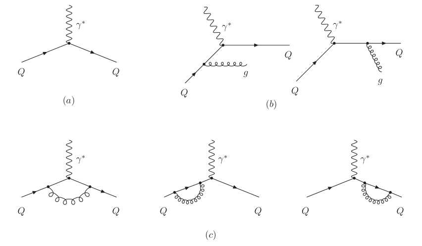
Figure 2: The LO (a) and NLO (b and c) photon-quark scattering diagrams.

At leading order, ${\cal O}(\alpha_{em})$, the only quark scattering subprocess is

$$\gamma^{*}(q)+Q(k_{Q})\rightarrow Q(p_{Q}).$$ (28)

The $\gamma^{*}Q$ cross sections, $\hat{\sigma}_{i}^{(0)}$ ($i=2,L,A,I$), corresponding to the Born diagram (see Fig. 2a) are:

$$\hat{\sigma}_{2}^{(0)}(z,\lambda) = \hat{\sigma}_{B}(z)\sqrt{1+4\lambda z^{2}}\,\delta(1-z),$$

$$\hat{\sigma}_{L}^{(0)}(z,\lambda) = \hat{\sigma}_{B}(z)\frac{4\lambda z^{2}}{\sqrt{1+4\lambda z^{2}}}\,\delta(1-z),$$ (29)

$$\hat{\sigma}_{A}^{(0)}(z,\lambda) = \hat{\sigma}_{I}^{(0)}(z,\lambda)=0,$$

with

$$\hat{\sigma}_{B}(z)=\frac{(2\pi)^{2}e_{Q}^{2}\alpha_{em}}{Q^{2}}\,z,$$ (30)

where $e_{Q}$ is the quark charge in units of electromagnetic coupling constant.

To take into account the NLO ${\cal O}(\alpha_{em}\alpha_{s})$ contributions, one needs to calculate the virtual corrections to the Born process (given in Fig. 2c) as well as the real gluon emission (see Fig. 2b):

$$\gamma^{*}(q)+Q(k_{Q})\rightarrow Q(p_{Q})+g(p_{g}).$$ (31)

The NLO $\varphi$-dependent cross sections, $\hat{\sigma}_{A}^{(1)}$ and $\hat{\sigma}_{I}^{(1)}$, are described by the real gluon emission only. Corresponding contributions are free of any type of singularities and the quantities $\hat{\sigma}_{A}^{(1)}$ and $\hat{\sigma}_{I}^{(1)}$ can be calculated directly in four dimensions.

In the $\varphi$-independent case, $\hat{\sigma}_{2}^{(1)}$ and $\hat{\sigma}_{L}^{(1)}$, we also work in four dimensions. The virtual contribution (Fig. 2c) contains ultraviolet (UV) singularity that is removed using the on-mass-shell regularization scheme. In particular, we calculate the absorptive part of the Feynman diagram which has no UV divergences. The real part is then obtained by using the appropriate dispersion relations. As to the infrared (IR) singularity, it is regularized with the help of an infinitesimal gluon mass. This IR divergence is cancelled when we add the bremsstrahlung contribution (Fig. 2b).

The final (real+virtual) results for $\gamma^{*}Q$ cross sections can be cast into the following form:

$$\hat{\sigma}_{2}^{(1)}(z,\lambda)=\frac{\alpha_{s}}{2\pi}C_{F}\hat{\sigma}_{B}(1)\sqrt{1+4\lambda}\,\delta(1-z)\Bigl{\{}-2+4\ln\lambda-\sqrt{1+4\lambda}\,\ln r+\frac{1+2\lambda}{\sqrt{1+4\lambda}}\Bigl{[}2\text{Li}_{2}(r^{2})+4\text{Li}_{2}(-r)$$

$$+3\ln^{2}(r)-4\ln r+4\ln r\ln(1+4\lambda)-2\ln r\ln\lambda\Bigr{]}\Bigr{\}}$$

$$+\frac{\alpha_{s}}{4\pi}C_{F}\hat{\sigma}_{B}(z)\frac{1}{(1+4\lambda z^{2})^{3/2}}\biggl{\{}\frac{1}{\left[1-(1-\lambda)z\right]^{2}}\Bigl{[}1-3z-4z^{2}+6z^{3}+8z^{4}-8z^{5}\qquad\qquad\qquad\;$$

$$+6\lambda z\left(3-18z+13z^{2}+10z^{3}-8z^{4}\right)\qquad\qquad$$

$$+4\lambda^{2}z^{2}\left(8-77z+65z^{2}-2z^{3}\right)\biggr{.}\qquad\qquad\qquad\;\,$$ (32)

$$+16\lambda^{3}z^{3}\left(1-21z+12z^{2}\right)-128\lambda^{4}z^{5}\Bigr{]}\qquad\quad\;\,$$

$$+\frac{2\ln D(z,\lambda)}{\sqrt{1+4\lambda z^{2}}}\Bigl{[}-\left(1+z+2z^{2}+2z^{3}\right)+2\lambda z\left(2-11z-11z^{2}\right)+8\lambda^{2}z^{2}\left(1-9z\right)\Bigr{]}$$

$$-\frac{8(1+4\lambda)^{2}z^{4}}{\left(1-z\right)_{+}}-\frac{4(1+2\lambda)(1+4\lambda)^{2}z^{4}}{\sqrt{1+4\lambda z^{2}}}\frac{\ln D(z,\lambda)}{\left(1-z\right)_{+}}\biggr{\}},$$

$$\hat{\sigma}_{L}^{(1)}(z,\lambda)=\frac{\alpha_{s}}{\pi}C_{F}\hat{\sigma}_{B}(1)\frac{2\lambda}{\sqrt{1+4\lambda}}\delta(1-z)\Bigl{\{}-2+4\ln\lambda-\frac{4\lambda}{\sqrt{1+4\lambda}}\,\ln r+\frac{1+2\lambda}{\sqrt{1+4\lambda}}\Bigl{[}2\text{Li}_{2}(r^{2})+4\text{Li}_{2}(-r)$$

$$+3\ln^{2}(r)-4\ln r+4\ln r\ln(1+4\lambda)-2\ln r\ln\lambda\Bigr{]}\Bigr{\}}$$

$$+\frac{\alpha_{s}}{\pi}C_{F}\hat{\sigma}_{B}(z)\frac{1}{(1+4\lambda z^{2})^{3/2}}\biggl{\{}\frac{z}{\left[1-(1-\lambda)z\right]^{2}}\Bigl{[}(1-z)^{2}-\lambda z\left(13-19z-2z^{2}+8z^{3}\right)\Bigr{.}\qquad\qquad$$

$$-2\lambda^{2}z^{2}\left(31-39z+8z^{2}\right)\Bigr{.}\qquad\qquad\qquad\qquad\quad\;\,$$ (33)

$$-8\lambda^{3}z^{3}\left(10-7z\right)-32\lambda^{4}z^{4}\Bigr{]}\Bigr{.}\qquad\qquad\qquad\qquad$$

$$-\frac{2\lambda z^{2}\ln D(z,\lambda)}{\sqrt{1+4\lambda z^{2}}}\left[3+3z+16\lambda z\right]\Bigr{.}\qquad\qquad\qquad\qquad\;\,$$

$$-\frac{8\lambda(1+4\lambda)z^{4}}{\left(1-z\right)_{+}}-\frac{4\lambda(1+2\lambda)(1+4\lambda)z^{4}}{\sqrt{1+4\lambda z^{2}}}\frac{\ln D(z,\lambda)}{\left(1-z\right)_{+}}\biggr{\}},$$

$$\hat{\sigma}_{A}^{(1)}(z,\lambda)=\frac{\alpha_{s}}{2\pi}C_{F}\hat{\sigma}_{B}(z)\frac{z(1-z)}{(1+4\lambda z^{2})^{3/2}}\biggl{\{}\frac{1}{\left[1-(1-\lambda)z\right]}\left[1+2\lambda(4-3z)+8\lambda^{2}z\right]+\frac{2\lambda\ln D(z,\lambda)}{\sqrt{1+4\lambda z^{2}}}\left[2+z+4\lambda z\right]\biggr{\}},$$ (34)

$$\hat{\sigma}_{I}^{(1)}(z,\lambda)=\frac{\alpha_{s}}{8\sqrt{2}}C_{F}\hat{\sigma}_{B}(z)\frac{1}{(1+4\lambda z^{2})^{2}}\frac{\sqrt{z}}{\left[1-(1-\lambda)z\right]^{3/2}}\biggl{\{}-(1-z)(1+2z)-4\lambda z\left(10-10z-z^{2}+2z^{3}\right)\qquad\quad\;\;$$

$$-8\lambda^{2}z^{2}\left(25-29z+8z^{2}\right)-96\lambda^{3}z^{3}\left(3-2z\right)-128\lambda^{4}z^{4}\biggr{.}\;$$ (35)

$$+8\sqrt{\lambda z\left[1-(1-\lambda)z\right]}\left[1-z^{2}+\lambda z(13-11z)+4\lambda^{2}z^{2}(7-4z)+16\lambda^{3}z^{3}\right]\biggr{\}}.$$

In Eqs. (32-35), $C_{F}=(N_{c}^{2}-1)/(2N_{c})$, where $N_{c}$ is number of colors, while

$$D(z,\lambda)=\frac{1+2\lambda z-\sqrt{1+4\lambda z^{2}}}{1+2\lambda z+\sqrt{1+4\lambda z^{2}}},\qquad\qquad\qquad\qquad\qquad r=\sqrt{D(z=1,\lambda)}=\frac{\sqrt{1+4\lambda}-1}{\sqrt{1+4\lambda}+1}.$$ (36)

The so-called ”plus” distributions are defined by

$$\left[g(z)\right]_{+}=g(z)-\delta(1-z)\int\limits_{0}^{1}\text{d}\zeta\,g(\zeta).$$ (37)

For any sufficiently regular test function $h(z)$, Eq. (37) gives

$$\int\limits_{a}^{1}\text{d}z\,h(z)\left[\frac{\ln^{k}(1-z)}{1-z}\right]_{+}=\int\limits_{a}^{1}\text{d}z\frac{\ln^{k}(1-z)}{1-z}\left[h(z)-h(1)\right]+h(1)\frac{\ln^{k+1}(1-a)}{k+1}.$$ (38)

IV Comparison with Available Results

For the first time, the NLO ${\cal O}(\alpha_{em}\alpha_{s})$ corrections to the $\varphi$-independent IC contribution have been calculated a long time ago by Hoffmann and Moore (HM) HM . However, authors of Ref. HM don’t give explicitly their definition of the partonic cross sections that leads to a confusion in interpretation of the original HM results. To clarify the situation, we need first to derive the relation between the lepton-quark DIS cross section, $\text{d}\hat{\sigma}_{lQ}$, and the partonic cross sections, $\sigma^{(2)}$ and $\sigma^{(L)}$, used in HM . Using Eqs. (C.1) and (C.5) in Ref. HM , one can express the HM tensor $\sigma_{R}^{\mu\nu}$ in terms of ”our” cross sections $\hat{\sigma}_{2}$ and $\hat{\sigma}_{L}$ defined by Eq. (27) in the present paper. Comparing the obtained results with the corresponding definition of $\sigma_{R}^{\mu\nu}$ via the HM cross sections $\sigma^{(2)}$ and $\sigma^{(L)}$ (given by Eqs. (C.16) and (C.17) in Ref. HM ), we find that

$$\hat{\sigma}_{2}(z,\lambda) \equiv \hat{\sigma}_{B}(z)\sqrt{1+4\lambda z^{2}}\,\sigma^{(2)}(z,\lambda),$$ (39)

$$\hat{\sigma}_{L}(z,\lambda) \equiv \frac{2\hat{\sigma}_{B}(z)}{\sqrt{1+4\lambda z^{2}}}\left[\sigma^{(L)}(z,\lambda)+2\lambda z^{2}\sigma^{(2)}(z,\lambda)\right].$$ (40)

Now we are able to compare our results with original HM ones. It is easy to see that the LO cross sections (defined by Eqs. (37) in HM and Eqs. (29) in our paper) obey both above identities. Comparing with each other the quantities $\sigma^{(2)}_{1}$ and $\hat{\sigma}_{2}^{(1)}$ (given by Eq. (51) in HM and Eq. (32) in this paper, respectively), we find that identity (39) is satisfied at NLO too. The situation with longitudinal cross sections is more complicated. We have uncovered two misprints in the NLO expression for $\sigma^{(L)}$ given by Eq. (52) in HM . First, the r.h.s. of this Eq. must be multiplied by $z$. Second, the sign in front of the last term (proportional to $\delta(1-z)$) in Eq. (52) in Ref. HM must be changed . Taking into account these typos, we find that relation (40) holds at NLO as well. So, our calculations of $\hat{\sigma}_{2}$ and $\hat{\sigma}_{L}$ agree with the HM results.

Recently, the heavy quark initiated contributions to the $\varphi$-independent DIS structure functions, $F_{2}$ and $F_{L}$, have been calculated by Kretzer and Schienbein (KS) KS . The final KS results are expressed in terms of the parton level structure functions $\hat{H}^{q}_{1}$ and $\hat{H}^{q}_{2}$. Using the definition of $\hat{H}^{q}_{1}$ and $\hat{H}^{q}_{2}$ given by Eqs. (7,8) in Ref. KS , we obtain that

$$\hat{\sigma}_{T}(z,\lambda)\equiv\frac{\alpha_{s}}{2\pi}\frac{\hat{\sigma}_{B}(z)}{\sqrt{1+4\lambda}}\frac{\hat{H}^{q}_{1}(\xi^{\prime},\lambda)}{\sqrt{1+4\lambda z^{2}}},\qquad\qquad\qquad\qquad\hat{\sigma}_{2}(z,\lambda)\equiv\frac{\alpha_{s}}{2\pi}\hat{\sigma}_{B}(z)\sqrt{\frac{1+4\lambda}{1+4\lambda z^{2}}}\,\hat{H}^{q}_{2}(\xi^{\prime},\lambda),$$ (41)

where $\hat{\sigma}_{T}=\hat{\sigma}_{2}-\hat{\sigma}_{L}$ and $\hat{\sigma}_{L}$ are defined by Eq. (27) in our paper and $\xi^{\prime}=z\left(1+\sqrt{1+4\lambda}\right)\left/\left(1+\sqrt{1+4\lambda z^{2}}\right)\right.$. To test identities (41), one needs only to rewrite the NLO expressions for the functions $\hat{H}^{q}_{1}(\xi^{\prime},\lambda)$ and $\hat{H}^{q}_{2}(\xi^{\prime},\lambda)$ (given in Appendix C in Ref. KS ) in terms of variables $z$ and $\lambda$. Our analysis shows that relations (41) hold at both LO and NLO. Hence we coincide with the KS predictions for the $\gamma^{*}Q$ cross sections.

However, we disagree with the conclusion of Refs. KS ; KS-thesis that there are errors in the NLO expression for $\sigma^{(2)}$ given in Ref. HM . As explained above, a correct interpretation of the quantities $\sigma^{(2)}$ and $\sigma^{(L)}$ used in HM leads to a complete agreement between the HM, KS and our results for $\varphi$-independent cross sections.

As to the $\varphi$-dependent DIS, pQCD predictions for the $\gamma^{*}Q$ cross sections $\hat{\sigma}_{A}(z,\lambda)$ and $\hat{\sigma}_{I}(z,\lambda)$ in the case of arbitrary values of $m^{2}$ and $Q^{2}$ are not, to our knowledge, available in the literature. For this reason, we have performed several cross checks of our results against well known calculations in two limits: $m^{2}\rightarrow 0$ and $Q^{2}\rightarrow 0$. In particular, in the chiral limit, we reproduce the original results of Georgi and Politzer GP and Méndez Mendez for $\hat{\sigma}_{I}(z,\lambda\rightarrow 0)$ and $\hat{\sigma}_{A}(z,\lambda\rightarrow 0)$. In the case of $Q^{2}\rightarrow 0$, our predictions for $\hat{\sigma}_{2}(s,Q^{2}\rightarrow 0)$ and $\hat{\sigma}_{A}(s,Q^{2}\rightarrow 0)$ given by Eqs. (32,34) reduce to the QED textbook results for the Compton scattering of polarized photons Fano .

V Some Properties of the Azimuth-Dependent Cross Sections

To perform a numerical investigation of the inclusive partonic cross sections, $\hat{\sigma}_{i}$ ($i=2,L,A,I$),  it is convenient to introduce the dimensionless coefficient functions $c_{i}^{(n,l)}$,

$$\hat{\sigma}_{i}(\eta,\lambda,\mu^{2})=\frac{e_{Q}^{2}\alpha_{em}\alpha_{s}(\mu^{2})}{m^{2}}\sum_{n=0}^{\infty}\left(4\pi\alpha_{s}(\mu^{2})\right)^{n}\sum_{l=0}^{n}c_{i}^{(n,l)}(\eta,\lambda)\ln^{l}\left(\frac{\mu^{2}}{m^{2}}\right),$$ (42)

where $\mu$ is a factorization scale (we use $\mu=\mu_{F}=\mu_{R}$) and the variable $\eta$ measures the distance to the partonic threshold:

$$\eta=\frac{s}{m^{2}}-1=\frac{1-z}{\lambda z},\qquad\qquad\qquad\qquad\qquad s=(q+k)^{2}.$$ (43)

Our analysis of the quantity $c_{A}^{(0,0)}(\eta,\lambda)$ is given in Fig. 3. One can see that $c_{A}^{(0,0)}$ is negative at low $Q^{2}$ ($\lambda^{-1}\lesssim 1$) and positive at high $Q^{2}$ ($\lambda^{-1}>20$). For the intermediate values of $Q^{2}$, $c_{A}^{(0,0)}(\eta,\lambda)$ is an alternating function of $\eta$.

Figure 3: $c_{A}^{(0,0)}(\eta,\lambda)$ and $c_{I}^{(0,0)}(\eta,\lambda)$ coefficient functions at several values of $\lambda$.

Let us discuss the coefficient function $c_{A}^{(0,0)}(s,Q^{2})$ for the case of on-mass-shell photon, $Q^{2}\rightarrow 0$. In this limit,

$$c_{A}^{(0,0)}(s,Q^{2}\rightarrow 0)=8\pi C_{F}\frac{m^{4}}{(s-m^{2})^{2}}\left[2+\frac{s+m^{2}}{s-m^{2}}\ln\frac{m^{2}}{s}\right]+{\cal{O}}(Q^{2}).$$ (44)

Considering now the threshold behavior of Eq. (44), we find: $\displaystyle{\lim_{s\rightarrow m^{2}}}c_{A}^{(0,0)}(s,Q^{2}\rightarrow 0)=-4\pi C_{F}/3$. Taking also into account that $\displaystyle{\lim_{s\rightarrow m^{2}}}c_{A}^{(0,0)}(s,Q^{2}\neq 0)=0$, we see that the mass-shell, $Q^{2}\rightarrow 0$, and threshold, $s\rightarrow m^{2}$, limits do not commutate with each other for the quantity $c_{A}^{(0,0)}(s,Q^{2})$. This property of the cross section $c_{A}^{(0,0)}(s,Q^{2})$ illustrates the well-known fact that there is no, generally speaking, a smooth transition between the lepto- and photoproduction.

Our results for the coefficient function $c_{I}^{(0,0)}(\eta,\lambda)$ at several values of $\lambda$ are presented in Fig. 3. It is seen that $c_{I}^{(0,0)}$ is negative at all values of $\eta$ and $\lambda$. Note also the threshold behavior of the coefficient function:

$$c_{I}^{(0,0)}(\eta\rightarrow 0,\lambda)=-\sqrt{2}\,\pi^{2}C_{F}\frac{\sqrt{\lambda}}{1+4\lambda}+{\cal{O}}(\eta).$$ (45)

This quantity takes its minimum value at $\lambda_{m}=1/4$: $c_{I}^{(0,0)}(\eta=0,\lambda_{m})=-\pi^{2}C_{F}/\left(2\sqrt{2}\right)$.

In the chiral limit, $m^{2}\rightarrow 0$, the $\varphi$-dependent cross section are as follows:

$$c_{A}^{(0,0)}(z,\lambda\rightarrow 0)=2\pi C_{F}\lambda z^{2}+{\cal{O}}(\lambda^{2}),\qquad\qquad\qquad c_{I}^{(0,0)}(z,\lambda\rightarrow 0)=-\frac{\sqrt{2}}{4}\pi^{2}C_{F}\lambda z(1+2z)\sqrt{\frac{z}{1-z}}+{\cal{O}}(\lambda^{2}).$$ (46)

Let us analyze the numerical significance of the $\cos\varphi$- and $\cos 2\varphi$-distributions for the QS component. It is difficult to compare directly the $\hat{\sigma}^{(1)}_{A}(z,\lambda)$ and $\hat{\sigma}^{(1)}_{I}(z,\lambda)$ cross section given by the usual functions (34) and (35) with the $\varphi$-independent contributions $\hat{\sigma}^{(0)}_{2}(z,\lambda)$ and $\hat{\sigma}^{(1)}_{2}(z,\lambda)$ described by the generalized functions (29) and (32). For this reason, we consider the Mellin moments of the corresponding quantities defined as

$$\hat{\sigma}_{i}(N,\lambda)=\int\limits^{1}_{0}\hat{\sigma}_{i}(z,\lambda)z^{N-1}\text{d}z,\qquad\qquad\qquad(i=2,L,A,I).$$ (47)

The Mellin transform of the Born level cross sections is trivial: $\hat{\sigma}^{(0)}_{2}(N,\lambda)=\hat{\sigma}_{B}(1)\sqrt{1+4\lambda}$. The Mellin moments of the NLO results have been calculated numerically. We use for $\alpha_{s}(\mu_{F})$ the one-loop approximation with $\Lambda_{4}=326$ MeV, $\mu_{F}=\sqrt{m^{2}+Q^{2}}$ and $m=1.3$ GeV.

Figure 4: The quantities $\hat{\sigma}^{(1)}_{A}(N,\lambda)/\hat{\sigma}^{(0)}_{2}(N,\lambda)$ (left panel) and $2\sqrt{2}\,\hat{\sigma}^{(1)}_{I}(N,\lambda)/\hat{\sigma}^{(0)}_{2}(N,\lambda)$ (right panel) at several values of $\lambda$.

The left panel of Fig. 4 presents the ratio $\hat{\sigma}^{(1)}_{A}(N,\lambda)/\hat{\sigma}^{(0)}_{2}(N,\lambda)$ as a function of $N$ for several values of variable $\lambda$: $\lambda^{-1}=1,4,10,20$ and 100. One can see that this ratio is negligibly small (of the order of 1$\%$). Moreover, our analysis shows that the ratio $\hat{\sigma}^{(1)}_{A}(N,\lambda)/\hat{\sigma}^{(0)}_{2}(N,\lambda)$ is less than $1.5\%$ for all values of $\lambda$ and $N>0$. This implies that the photon-quark scattering contribution is practically $\cos 2\varphi$-independent.

In the right panel of Fig. 4, the $N$-dependence of the ratio $2\sqrt{2}\,\hat{\sigma}^{(1)}_{I}(N,\lambda)/\hat{\sigma}^{(0)}_{2}(N,\lambda)$ is given for the same values of $\lambda$. One can see that this ratio is of the order of 10-15$\%$ at small $N$ and sufficiently high $Q^{2}$. This fact indicates that the $\cos\varphi$-distribution caused by the QS component may be sizable.

VI Conclusion

We conclude by summarizing our main observations. In the present paper, we have studied the azimuth-dependent photon-(heavy) quark DIS at NLO. It turns out that the $\cos 2\varphi$ dependence of the QS mechanism is negligible while the $\cos\varphi$ one may be sizable. The situation is diametrically opposite to the one that takes place for the basic GF contribution. It is well known that the GF predictions for the azimuthal $\cos 2\varphi$ asymmetry in heavy quark photo- Duke-Owens ; we1 and leptoproduction LW1 ; Watson ; we4 are large (about 20$\%$). As to the $\cos\varphi$ dependence of the GF contribution, it vanishes at LO due to the charge symmetry $Q\leftrightarrow\overline{Q}$ LW2 .

Since the GF and QS mechanisms have strongly different azimuthal distributions, one could expect that measurements of the $\varphi$-dependent DIS will directly probe the charm content of the proton. In detail, hadron level predictions for the azimuthal asymmetries as well as the possibility to discriminate experimentally between the GF and QS contributions will be investigated in Ref. we5 .

References

(1) S. J. Brodsky, P. Hoyer, C. Peterson, and N. Sakai,
Phys. Lett. B 93, 451 (1980).
(2) S. J. Brodsky, C. Peterson, and N. Sakai,
Phys. Rev. D 23, 2745 (1981).
(3) S. J. Brodsky, ”Light-front QCD”, hep-ph/0412101.
(4) S. J. Brodsky, Few Body Syst. 36, 35 (2005).
(5) M. Franz, V. Polyakov, and K. Goeke,
Phys. Rev. D 62, 074024 (2000).
(6) M. A. G. Aivazis, J. C. Collins, F. I. Olness, and W. -K. Tung,
Phys. Rev. D 50, 3102 (1994).
(7) J. C. Collins, Phys. Rev. D 58, 094002 (1998).
(8) R. S. Thorne, Phys. Rev. D 73, 054019 (2006).
(9) W. K. Tung, H .L. Lai, A. Belyaev, J. Pumplin, D. Stump,
and C. -P. Yuan, hep-ph/0611254.
(10) S. Kretzer, H. L. Lai, F. I. Olness and W. -K. Tung,
Phys. Rev. D 69, 114005 (2004).
(11) W. -K. Tung, S. Kretzer, and C. Schmidt, J. Phys. G 28, 983 (2002).
(12) M. Kramer, F. I. Olness, and D. E. Soper,
Phys. Rev. D 62, 096007 (2000).
(13) J. Pumplin, Phys. Rev. D 73, 114015 (2006).
(14) S. J. Brodsky, B. Kopeliovich, I. Schmidt, and J. Soffer,
Phys. Rev. D 73, 113005 (2006).
(15) J. Pumplin, D. R. Stump, J. Huston, H. L. Lai, P. Nadolsky,
and W. K. Tung, JHEP 0207, 012 (2002).
(16) A. D. Martin, R. G. Roberts, W. J. Stirling, and R. S. Thorne,
Phys. Lett. B 604, 61 (2004).
(17) M. L. Mangano, P. Nason, and G. Ridolfi,
Nucl. Phys. B 373, 295 (1992).
(18) S. Frixione, M. L. Mangano, P. Nason, and G. Ridolfi,
Nucl. Phys. B 412, 225 (1994).
(19) R. K. Ellis and P. Nason, Nucl. Phys. B 312, 551 (1989).
(20) J. Smith and W. L. van Neerven,
Nucl. Phys. B 374, 36 (1992).
(21) E. Laenen, S. Riemersma, J. Smith, and W. L. van Neerven,
Nucl. Phys. B 392, 162 (1993).
(22) W. Beenakker, H. Kuijf, W. L. van Neerven, and J. Smith,
Phys. Rev. D 40, 54 (1989).
(23) P. Nason, S. Dawson, and R. K. Ellis,
Nucl. Phys. B 303, 607 (1988).
(24) P. Nason, S. Dawson, and R. K. Ellis,
Nucl. Phys. B 327, 49 (1989).
(25) P. Nason, S. Dawson, and R. K. Ellis,
Nucl. Phys. B 335, 260 (1990).
(26) H. Contopanagos, E. Laenen, and G. Sterman,
Nucl. Phys. B 484, 303 (1997).
(27) E. Laenen, G. Oderda, and G. Sterman,
Phys. Lett. B 438, 173 (1998).
(28) N. Kidonakis, G. Oderda, and G. Sterman,
Nucl. Phys. B 531, 365 (1998).
(29) E. Laenen and S. -O. Moch, Phys. Rev. D 59, 034027 (1999).
(30) N. Kidonakis, Phys. Rev. D 73, 034001 (2006).
(31) N. Kidonakis, Phys. Rev. D 64, 014009 (2001).
(32) N. Ya. Ivanov, A. Capella, and A. B. Kaidalov,
Nucl. Phys. B 586, 382 (2000).
(33) N. Ya. Ivanov, Nucl. Phys. B 615, 266 (2001).
(34) N. Ya. Ivanov, Nucl. Phys. B 666, 88 (2003).
(35) N. Ya. Ivanov, P. E. Bosted, K. Griffioen, and S. E. Rock,
Nucl. Phys. B 650, 271 (2003).
(36) E. Hoffman and R. Moore, Z. Phys. C 20, 71 (1983).
(37) S. Kretzer and I. Schienbein, Phys. Rev. D 58, 094035 (1998).
(38) I. Schienbein, hep-ph/0110292.
(39) L. N. Ananikyan and N. Ya. Ivanov, Nucl. Phys. B 762,
256 (2007).
(40) A. Deshpande, R. Milner, R. Venugopalan, and W. Vogelsang,
Ann. Rev. Nucl. Part. Sci. 55, 165 (2005).
(41) See also http://www.bnl.gov/eic for information concernig
the eRHIC/EIC project.
(42) J. B. Dainton, M. Klein, P. Newman, E. Perez, and F. Willeke,
hep-ex/0603016.
(43) M. A. G. Aivazis, F. I. Olness, and W. -K. Tung,
Phys. Rev. D 50, 3085 (1994).
(44) N. Dombey, Rev. Mod. Phys. 41, 236 (1969).
(45) H. Georgi and H. D. Politzer, Phys. Rev. Lett. 40, 3 (1978).
(46) A. Méndez, Nucl. Phys. B 145, 199 (1978).
(47) U. Fano, Phys. Rev. 93, 121 (1954).
(48) D. W. Duke and J. F. Owens,
Phys. Rev. Lett. 44, 1173 (1980).
(49) J. P. Leveille and T. Weiler, Phys. Rev. D 24, 1789 (1981).
(50) A. D. Watson, Z. Phys. C 12, 123 (1982).
(51) J. P. Leveille and T. Weiler, Nucl. Phys. B 147, 147 (1979).