Covariant light-front approach for heavy quarkonium:

decay constants, $P\to\gamma\gamma$ and $V\to P\gamma$

Chien-Wen Hwang^a,b and Zheng-Tao Wei^b,c,d

^a Department of Physics, National Kaohsiung Normal University, Kaohsiung 802, Taiwan

^b National Center for Theoretical Sciences, National Cheng-Kung University, Tainan 701, Taiwan

^c Institute of Physics, Academia Sinica, Taipei 115, Taiwan

^d Department of Physics, Nankai University, Tianjin 300071, China

Abstract

The light-front approach is a relativistic quark model and offers many insights to the internal structures of the hadronic bound states. In this study, we apply the covariant light-front approach to ground-state heavy quarkonium. The pesudoscalar and vector meson decay constants are discussed. We present a detailed study of two-photon annihilation $P\to\gamma\gamma$ and magnetic dipole transition $V\to P\gamma$ processes. The numerical predictions of the light-front approach are consistent with the experimental data and those in other approaches. The relations of the light-front approach with the other methods are discussed in brief.

I Introduction

Heavy quarkonium provides a unique laboratory to study Quantum Chromodynamics (QCD) for the bound states of heavy quark-antiquark system. The nature that the heavy quarkonium is relevant to a non-relativistic treatment had been known for a long time QR . Although the non-relativistic QCD (NRQCD), an effective field theory, is a powerful theoretical tool to separate the high energy modes from the low energy contributions, the calculations of the low energy hadronic matrix elements rely on model-dependent non-perturbative methods in most cases. From the point of view of the non-perturbative QCD, there is no one method which is uniquely superior over the others. Many methods were employed in heavy quarkonium physics, such as lattice QCD, quark-potential model, etc. (for a recent review see HQ ). The light-front quark model, in which a hadronic matrix element is represented as the overlap of wave functions, offers many insights into the internal structures of the bound states. In this study, we will explore the heavy quarkonium from a quark model on the light front.

The light-front QCD has been developed as a promising analytic method for solving the non-perturbative problems of hadron physics BPP . The aim of the light-front QCD is to describe the hadronic bound states in terms of their fundamental quark and gluon degrees of freedom. It may be the only possible method that the low energy quark model and the high energy parton model can be reconciled. For the hard processes with large momentum transferred, the light-front QCD reduces to perturbative QCD (pQCD) which factorize the physical quantity into a convolution of the hard scattering kernel and the distribution amplitudes (or functions). In general, the basic ingredient in light-front QCD is the relativistic hadron wave functions which generalize the distribution amplitudes (or functions) by including the transverse momentum distributions. It contains all information of a hadron from its constituents. The hadronic quantities are represented by the overlaps of wave functions and can be derived in principle.

The light-front quark model is the only relativistic quark model in which a consistent and fully relativistic treatment of quark spins and the center-of-mass motion can be carried out LFQM . This model has many advantages. For example, the light-front wave function is manifestly Lorentz invariant as it is expressed in terms of the internal momentum fraction variables which is independent of the total hadron momentum. Moreover, hadron spin can also be correctly constructed using the so-called Melosh rotation. This model had been successfully applied to calculate many phenomenologically important meson decay constants and hadronic form factors Jaus1 ; CCH1 ; Jaus2 ; CCH2 ; Hwang .

On the light front, the non-relativistic nature of a heavy quarkonium is represented by that the light-front momentum fractions of the quark and antiquark is close to $1/2$ and the relative transverse and the $z-$direction momenta are much smaller than the heavy quark mass. The Lorentz invariant light-front wave function and the light-front formulations provide a systematic way to include the relativistic corrections. There is no conceptual problem to extend the light-front approach into the heavy quarkonium. We will apply the covariant light-front approach Jaus2 ; CCH2 to the ground-state $s$-wave mesons which include ${}^{1}S_{0}$ pseudoscalar mesons ($P$) $\eta_{c},\eta_{b}$ and ${}^{3}S_{1}$ vector mesons ($V$) $J/\psi,\Upsilon(1S)$ as our first-step study along this direction. The main purposes of this study are threefold: (1) Is the light-front approach applicable into the heavy quarkonium? In concept, the light-front quark model is the relativistic generalization of the non-relativistic quark model. The phenomenological success of the previous non-relativistic quark-potential model should be reproduced in the light-front approach. In particular, we will examine the validity of the light-front approach in three types of quantities: decay constants, two-photon annihilation $P\to\gamma\gamma$ and magnetic dipole transition $V\to P\gamma$. In most literatures, these processes were explored separately KMRR ; AB ; BJV ; DER . To study them simultaneously can better constrain the phenomenological parameters and check the consistency of the theory predictions. (2) The $\eta_{b}$ meson has still not been observed in experiment ALEPH . We will present the numerical prediction for the branching ratios for $\eta_{b}\to\gamma\gamma$ and $\Upsilon\to\eta_{b}\gamma$ processes. (3) What is the relation of the light-front approach with the other approaches? In the non-relativistic approximations, the light-front approach will be closely related with the non-relativistic quark-potential approach. For the process of $P\to\gamma\gamma$ which is light-front dominated, the light-front approach reduce to the model-independent pQCD.

The paper is organized as follows. In Sec. II, we give a detailed presentation of the covariant light-front approach for heavy quarkonium. It contains a brief review of the light-front framework and the light-front analysis for the decay constants of $P$ and $V$ mesons and the processes $P\to\gamma\gamma$, $V\to P\gamma$. In Sec. III, the relations of the light-front approach with the non-relativistic approach and pQCD are discussed. In Sec. IV, the numerical results and discussions are presented. Finally, the conclusions are given in Sec. V.

II Formalism of covariant light-front approach

II.1 General formalism

A heavy quarkonium is the hadronic bound state of heavy quark and antiquark. In this system, the valence quarks have equal masses $m_{1}=m_{2}=m$ with $m$ the mass of heavy quark $c$ or $b$. Thus the formulae associated with the term $(m_{1}-m_{2})$ vanish and will lead to some simplifications. In this section, we will give the formulae specially for the quarkonium system.

The momentum of a particle is given in terms of light-front component by $k=(k^{-},k^{+},k_{\perp})$ where $k^{\pm}=k^{0}\pm k^{3}$ and $k_{\perp}=(k^{1},k^{2})$, and the light-front vector is written as $\tilde{k}=(k^{+},k_{\perp})$. The longitudinal component $k^{+}$ is restricted to be positive, i.e., $k^{+}>0$ for the massive particle. By this way, the physical vacuum of light-front QCD is trivial except the zero longitudinal momentum modes (zero-mode). We will study a meson with total momentum $P$ and two constituents, quark and antiquark whose momenta are $p_{1}$ and $p_{2}$, respectively. In order to describe the internal motion of the constituents, it is crucial to introduce the intrinsic variables $(x_{i},p_{\perp})$ through

$$p_{1}^{+}=x_{1}P^{+},\qquad\qquad p_{1\perp}=x_{1}P_{\bot}+p_{\perp};$$

$$p_{2}^{+}=x_{2}P^{+},\qquad\qquad p_{2\perp}=x_{2}P_{\bot}-p_{\perp},$$ (1)

where $x_{i}$ are the light-front momentum fractions and they satisfy $0<x_{1},x_{2}<1$ and $x_{1}+x_{2}=1$. The invariant mass $M_{0}$ of the constituents and the relative momentum in $z$ direction $p_{z}$ can be written as

$$M_{0}^{2}=\frac{p_{\perp}^{2}+m^{2}}{x_{1}x_{2}},\qquad~{}~{}~{}p_{z}=(x_{2}-\frac{1}{2})M_{0}.$$ (2)

The invariant mass $M_{0}$ of $q\bar{q}$ is in general different from the mass $M$ of meson which satisfies $M^{2}=P^{2}$. This is due to the fact that the meson, quark and antiquark can not be on-shell simultaneously. The momenta $p_{\perp}$ and $p_{z}$ constitute a momentum vector $\vec{p}=(p_{\perp},p_{z})$ which represents the relative momenta in the transverse and $z$ directions, respectively. The energy of the quark and antiquark $e_{1}=e_{2}\equiv e$ can be obtained from their relative momenta,

$$e=\sqrt{m^{2}+p_{\perp}^{2}+p_{z}^{2}}.$$ (3)

It is straightforward to find that

$$x_{1}=\frac{e-p_{z}}{2e},~{}x_{2}=\frac{e+p_{z}}{2e},~{}e=\frac{M_{0}}{2}.$$ (4)

To calculate the decay constants or decay amplitude, the Feynman rules for the vertices of quark-antiquark coupling to the meson bound state are required. In the following formulations, we will follow the notations in CCH2 . The vertices $\Gamma_{M}$ for the incoming meson $M$ are given as

$$H_{P}\gamma_{5}\qquad\qquad\qquad\qquad {\rm for~{}}P;$$

$$iH_{V}\Big{[}\gamma_{\mu}-\frac{1}{W_{V}}(p_{1}-p_{2})_{\mu}\Big{]}\qquad {\rm for~{}}V.$$ (5)

After performing a one-loop contour integral to be discussed below which amounts to make one quark or antiquark on its mass-shell, the function $H_{M}$ and the parameter $W_{V}$ are reduced to $h_{M}$ and $w_{V}$, respectively, and they are written by

$$h_{P}=h_{V}=(M^{2}-M_{0}^{2})\sqrt{\frac{x_{1}x_{2}}{N_{c}}}\frac{1}{\sqrt{2}M_{0}}\phi(x_{2},p_{\bot}),$$ (6)

and

$$w_{V}=M_{0}+2m.$$ (7)

The form of the function $h_{M}$ and the Feynman rule for $\Gamma_{M}$ are derived from the light-front wave function which describes a meson bound state in terms of a quark $q_{1}$ and an antiquark $\bar{q}_{2}$. The light-front wave function contains two parts: one is the momentum distribution amplitude $\phi(x_{2},p_{\bot})$ which is the central ingredient in light-front QCD, the other is a spin wave function which constructs a state of definite spin ($S,S_{z}$) out of light front helicity eigenstates ($\lambda_{1},\lambda_{2}$). The spin wave function is constructed by using the Melosh transformation and its spin structure has been contained in Eq. (II.1).

The momentum distribution amplitude $\phi(x_{2},p_{\bot})$ is the generalization of the distribution amplitude $\phi(x)$ of the pQCD method and can be chosen to be normalizable, i.e., it satisfies

$$\int\frac{dxd^{2}p_{\bot}}{2(2\pi)^{3}}|\phi(x,p_{\bot})|^{2}=1.$$ (8)

In principle, $\phi(x_{2},p_{\bot})$ is obtained by solving the light-front QCD bound state equations $H_{LF}|\Psi\rangle=M|\Psi\rangle$ which is the familiar Schrödinger equation in ordinary quantum mechanics and $H_{LF}$ is the light-front Hamiltonian. To see the explicit form of the light-front bound state equation, let us consider a quarkonium wave function. The light-front bound state equation can be expressed as:

$$\begin{array}[]{l}\biggl{(}M^{2}-\displaystyle\sum_{i}\displaystyle\frac{\,k_{i\bot}^{2}+m^{2}_{i}\,}{x_{i}}\biggr{)}\left(\begin{array}[]{c}\Psi_{q\bar{q}}\\ \Psi_{q\bar{q}g}\\ \vdots\end{array}\right)\\[15.0pt] \hskip 22.76228pt=\left(\begin{array}[]{ccc}\langle q\bar{q}|H_{int}|q\bar{q}\rangle&\langle q\bar{q}|H_{int}|q\bar{q}g\rangle&\cdots\\ \langle q\bar{q}g|H_{int}|q\bar{q}\rangle&\cdots&\\ \vdots&&\end{array}\right)\left(\begin{array}[]{c}\Psi_{q\bar{q}}\\ \Psi_{q\bar{q}g}\\ \vdots\end{array}\right)\,.\end{array}$$ (9)

Of course, to exactly solve the above equation for the whole Fock space is still impossible. Currently, two approaches have been developed. One is given by Brodsky and Pauli PB ; TBP ; KP ; KPP , the so-called discretize light-front approach, the other by Perry, Harindranath and Wilson PHW ; PH ; GHPSW , based on the old idea of the Tamm-Dancoff approach T ; D that truncates the Fock space to only include these Fock states with a small number of particles. Furthermore, if one can eliminate all the high order Fock space sectors (approximately) by an effective two-body interaction kernel, the light-front bound state equation is reduced to the light-front Bethe-Salpeter equation:

$$\biggl{(}M^{2}-\displaystyle\frac{\,k_{\bot}^{2}+m^{2}\,}{\,x(1-x)\,}\biggr{)}\Psi_{q\bar{q}}(x,k_{\bot})=\displaystyle\int\displaystyle\frac{\,dyd^{2}k^{\prime}_{\bot}\,}{2(2\pi)^{3}}V_{eff}(x,k_{\bot},y,k^{\prime}_{\bot})\Psi_{q\bar{q}}(y,k^{\prime}_{\bot})\,.$$ (10)

One may solve the Bethe-Salpeter equation for finding the relativistic bound states. However, the Bethe-Salpeter equation only provides the amplitude of a Fock sector in the bound states so that it cannot be normalized. In other words, the Bethe-Salpeter amplitudes do not have the precise meaning of wave functions for particles. In addition, the advantage for Eq. (9) with the Tamm-Dancoff approximation is that it provides a reliable way to study the contribution of Fock states which contain more particles step by step by increasing the size of truncated Fock space, while the Bethe-Salpeter equation Eq. (10) lacks such an ability. Some studies on nonperturbative features of light-front dynamics were focused on the 1+1 field theory. Typical examples are: the discretized light-front quantization approach for the bound states in the 1+1 field theory developed by Pauli and Brodsky PB ; EPB , the light-front Tamm-Dancoff approach for bound state Fock space truncation discussed by Perry et al. PHW ; PH . However, at the present time, how to solve for the bound states from 3+1 QCD is still unknown. We are satisfied with utilizing some phenomenological momentum distribution amplitudes which have been constructed phenomenologically in describing hadrons. One widely used form is the Gaussian-type which we will employ in the application of covariant light-front approach.

II.2 Decay constants

In general, the decay constants of mesons $f_{P,V}$ are defined by the matrix elements for $P$ and $V$ mesons

$$\langle 0|A_{\mu}|P(P)\rangle = if_{P}P_{\mu},$$

$$\langle 0|V_{\mu}|V(P)\rangle = M_{V}f_{V}\epsilon_{\mu}.$$ (11)

where $P_{\mu}$ is the momentum of meson and $\epsilon_{\mu}$ is the polarization vector of $V$ meson. The Feynman diagram which contributes to $f_{P,V}$ is depicted in Fig. 1.

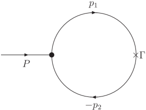
Figure 1: Feynman diagram for meson decay constants, where $P$ is the momentum of meson, $p_{1}$ is the quark momentum, $p_{2}$ is the antiquark momentum and $\Gamma$ denotes the corresponding $V$-$A$ current.

The meson decay constant plays an important role in determining the parameters of the distribution function $\phi(x_{2},p_{\bot})$, in particular, the quark mass and a parameter $\beta$ characterizing the hadronic “size” for a Gaussian wave function. The decay constants have been calculated in Jaus2 ; CCH2 and are the same as our results. Thus we simply provide the formulae for $f_{P,V}$ here.

For a pseudoscalar quarkonium, the decay constant is represented by

$$f_{P} = \frac{\sqrt{2N_{c}}}{8\pi^{3}}\int dx_{2}d^{2}p_{\perp}\frac{m}{\sqrt{x_{1}x_{2}}M_{0}}\phi_{P}(x_{2},p_{\bot})$$ (12)

$$= \frac{\sqrt{2N_{c}}}{8\pi^{3}}\int dx_{2}d^{2}p_{\perp}\frac{m}{\sqrt{m^{2}+p_{\perp}^{2}}}\phi_{P}(x_{2},p_{\bot}).$$

where $N_{c}=3$ is the color number and $m$ denotes the mass of the heavy quark. In Eq. (12), we have used the relation

$$M_{0}\sqrt{x_{1}x_{2}}=\sqrt{m^{2}+p_{\perp}^{2}}$$ (13)

for a quarkonium .

For the vector meson, the decay constant in the covariant approach is represented by

$$f_{V}=\frac{\sqrt{2N_{c}}}{8\pi^{3}M}\int dx_{2}d^{2}p_{\perp}\frac{1}{\sqrt{m^{2}+p_{\perp}^{2}}}\left[x_{1}M_{0}^{2}-p_{\perp}^{2}+\frac{2m}{w_{V}}p_{\perp}^{2}\right]\phi_{V}(x_{2},p_{\bot}).$$ (14)

Eq. (14) coincides with the result in Jaus2 when $m_{1}=m_{2}$. Note that the $1/w_{V}$ part of Eq. (14) is different from that in the conventional approach, for example, CCH1 . The reason is that the conventional approach is not covariant and contains a spurious dependence on the orientation of the light front. The relevant calculations are not free of spurious contributions for transitions involving vector meson. Zero modes, which relate to the $p^{-}$ integration for $p^{+}=0$, are required to eliminate the spurious dependence and contribute to the $1/w_{V}$ part of Eq. (14). More detailed discussions about this point can be found in Jaus2 ; CCH2 . The decay constant $f_{V}$ is related to the electromagnetic decay of vector meson $V\to e^{+}e^{-}$ by NS

$$\Gamma(V\to e^{+}e^{-})=\frac{4\pi}{3}\frac{\alpha^{2}}{M_{V}}c_{V}f_{V}^{2}.$$ (15)

where $c_{V}$ is factor related to the electric charge of the quark that make up the vector meson.

II.3 $P\to\gamma\gamma$

Charge conservation requires charge conjugation $C=+1$ state coupling to two photons. Thus only pseudoscalar meson can transform into two photons while the vector meson is forbidden. In the process of $P\to\gamma\gamma$, the final two photons are both on-shell. For the purpose of illustration, it is useful to consider a more general process $P\to\gamma\gamma^{*}$ with one photon off-shell. We introduce a transition form factor $F_{P\gamma}(q^{2})$ arising from the $P\gamma\gamma^{*}$ vertex. The $P\to\gamma\gamma$ process is related to the form factor at $q^{2}=0$, i.e., $F_{P\gamma}(0)$. The form factor $F_{P\gamma}(q^{2})$ is defined by

$${\cal A}_{\mu}=-ie^{2}F_{{P\gamma}}(q^{2})\epsilon_{\mu\nu\rho\sigma}P^{\nu}q_{1}^{\rho}\epsilon^{\sigma}.$$ (16)

where ${\cal A}_{\mu}$ is the decay amplitude of the process $P\to\gamma\gamma^{*}$ and $q_{1}(\epsilon)$ the momentum (polarization) of the on-shell photon.

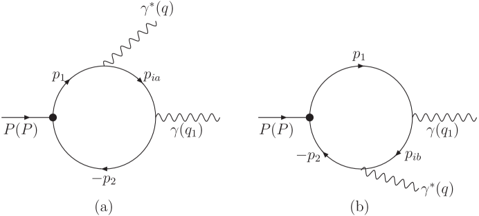
Figure 2: Feynman diagram for $P\to\gamma\gamma^{*}$ process where $P$ in the parenthesis denotes the momentum of meson. The diagram (b) is related to (a) by the exchange of two photons.

The transition amplitude for the process of $P\to\gamma\gamma^{*}$ can be derived from the common Feynman rules and the vertices for the meson-quark-antiquark coupling given in Eq. (II.1). In the covariant light-front approach, the meson is on-shell while the constituent quarks are off-shell and the momentum satisfies $P=p_{1}+p_{2}$. To the lowest order approximation, $P\to\gamma\gamma^{*}$ is a one-loop diagram and depicted in Fig. 2. The amplitude is given as a momentum integral

$${\cal A}_{\mu}=ie_{q}^{2}e^{2}N_{c}\int\frac{d^{4}p_{1}}{(2\pi)^{4}}\Big{\{}\frac{H_{P}}{N_{1}N_{2}N_{ia}}{\rm Tr}[{\gamma_{5}(-\not\!p_{2}+m)\not\!\epsilon(\not\!p_{ia}+m)\gamma_{\mu}}(\not\!p_{1}+m)]$$

$$+\frac{H_{P}}{N_{1}N_{2}N_{ib}}{\rm Tr}[{\gamma_{5}(-\not\!p_{2}+m)\gamma_{\mu}}(\not\!p_{ib}+m)\not\!\epsilon(\not\!p_{1}+m)]\Big{\}},$$ (17)

where

$$p_{ia}=p_{1}-q,~{}~{}~{}~{}~{}~{}~{}~{}~{}~{}~{}~{}~{}~{}~{}~{}~{} p_{ib}=q-p_{2},$$ (18)

$$N_{1}=p_{1}^{2}-m^{2}+i\epsilon,~{}~{}~{}~{}~{}~{}~{}~{}~{}~{} N_{2}=p_{2}^{2}-m^{2}+i\epsilon,$$

$$N_{ia}=p_{ia}^{2}-m^{2}+i\epsilon,~{}~{}~{}~{}~{}~{}~{}~{}~{}~{} N_{ib}=p_{ib}^{2}-m^{2}+i\epsilon,$$

and $e_{q}$ is the electric charge of quark: $e_{q}=2/3$ for $c$ quark and $e_{q}=-1/3$ for $b$ quark. The first and second terms in Eq. (II.3) come from diagrams Fig. 2 (a) and (b), respectively.

For the calculation of the form factor $F_{P\gamma}(q^{2})$, it is convenient to choose the purely transverse frame $q^{+}=0$, i.e., $q^{2}=-q_{\bot}^{2}\leq 0$. The advantage of this choice is that there is no the so-called Z-diagram contributions. The price is that only the form factor at space-like regions can be calculated directly. The values at the time-like momentum transfer $q^{2}>0$ regions are obtained by analytic continuation. In this study, the continuation is not necessary because we only need the form factors at $q^{2}=0$ for the $P\to\gamma\gamma$ and $V\to P\gamma$ processes.

At first, we discuss the calculation of Fig. 2(a). The factors $N_{1}$, $N_{2}$ and $N_{ia}$ produce three singularities in the $p_{1}^{-}$ complex plane: one lies in the upper plane; the other two in the lower plane. By closing the contour in the upper $p_{1}^{-}$ complex plane, the momentum integral can be easily calculated since there is only one singularity in the plane. This corresponds to putting the antiquark on the mass-shell. Given this restriction, the momentum $p_{2}\to\hat{p}_{2}$ with $\hat{p}_{2}^{2}-m^{2}=0$, and $\hat{p}_{1}=P-\hat{p}_{2}$. The on-shell restriction and the requirement of covariance lead to the following replacements:

$$N_{1} \to \hat{N}_{1}=x_{1}(M^{2}-M_{0}^{2}),$$

$$N_{ia} \to \hat{N}_{ia}=x_{2}q^{2}-x_{1}M_{0}^{2}+2p_{\bot}\cdot q_{\bot},$$

$$N_{2} \to \hat{N}_{2}=\hat{N}_{1}+(1-2x_{1})M^{2}=x_{2}M^{2}-x_{1}M_{0}^{2},$$

$$\int\frac{d^{4}p_{1}}{(2\pi)^{4}}\frac{H_{P}}{N_{1}N_{2}N_{ia}} \to -i\pi\int\frac{dx_{2}d^{2}p_{\bot}}{(2\pi)^{4}}\frac{h_{P}}{x_{2}\hat{N}_{1}\hat{N}_{ia}}.$$ (19)

For Fig. 2(b), the contour is closed in the lower $p_{1}^{-}$ complex plane. It corresponds to putting the quark on the mass-shell and the momentum $p_{1}\to\hat{p}_{1}$ with $\hat{p}_{1}^{2}-m^{2}=0$. In this case, we need to do the following replacements

$$N_{2} \to \hat{N}_{2}=x_{2}(M^{2}-M_{0}^{2}),$$

$$N_{ib} \to \hat{N}_{ib}=x_{1}q^{2}-x_{2}M_{0}^{2}-2p_{\bot}\cdot q_{\bot},$$

$$N_{1} \to \hat{N}_{1}=x_{1}M^{2}-x_{2}M_{0}^{2},$$

$$\int\frac{d^{4}p_{1}}{(2\pi)^{4}}\frac{H_{P}}{N_{1}N_{2}N_{ib}} \to -i\pi\int\frac{dx_{2}d^{2}p_{\bot}}{(2\pi)^{4}}\frac{h_{P}}{x_{1}\hat{N}_{2}\hat{N}_{ib}}.$$ (20)

From Eqs. (II.3) and (II.3), we see that $\hat{N}_{ib}$ is obtained from $\hat{N}_{ia}$ by the exchange of $x_{1}\leftrightarrow x_{2}$ and the change of the sign of $p_{\bot}$.

After the above treatments, the transition amplitude of $P\to\gamma\gamma^{*}$ is obtained as

$${\cal A}_{\mu}= -ie^{2}\epsilon_{\mu\nu\rho\sigma}P^{\nu}q_{1}^{\rho}\epsilon^{\sigma}\int\frac{dx_{2}d^{2}p_{\bot}}{4\pi^{3}}\frac{N_{c}e_{q}^{2}m~{}h_{P}}{x_{1}x_{2}(M^{2}-M_{0}^{2})}$$ (21)

$$~{}~{}~{}~{}\times\left[\frac{1}{-x_{2}q^{2}+x_{1}M_{0}^{2}-2p_{\bot}\cdot q_{\bot}}+\frac{1}{-x_{1}q^{2}+x_{2}M_{0}^{2}+2p_{\bot}\cdot q_{\bot}}\right],$$

Thus, the final formulae for the form factor $F_{P\gamma}(q^{2})$ is

$$F_{P\gamma}(q^{2})= \frac{e_{q}^{2}\sqrt{2N_{c}}}{8\pi^{3}}\int dx_{2}d^{2}p_{\bot}\phi_{P}(x_{2},p_{\bot})\frac{m}{\sqrt{m^{2}+p_{\bot}^{2}}}$$ (22)

$$~{}~{}~{}~{}\times\left[\frac{1}{x_{1}M_{0}^{2}-x_{2}q^{2}-2p_{\bot}\cdot q_{\bot}}+\frac{1}{x_{2}M_{0}^{2}-x_{1}q^{2}+2p_{\bot}\cdot q_{\bot}}\right],$$

and $F_{P\gamma}(0)$ is

$$F_{P\gamma}(0)=\frac{e_{q}^{2}\sqrt{2N_{c}}}{8\pi^{3}}\int dx_{2}d^{2}p_{\bot}\phi_{P}(x_{2},p_{\bot})\frac{m}{\sqrt{m^{2}+p_{\bot}^{2}}}\frac{1}{x_{1}x_{2}M_{0}^{2}}.$$ (23)

By comparing Eq. (23) with Eq. (12), they share some similarities except the propagators $N_{ia(b)}$ (and a trivial factor $e_{q}^{2}$). This point will become clearer when we discuss the relation between the light-front QCD and pQCD method.

The decay rate for $P\to\gamma\gamma$ is obtained from the transition form factors by

$$\Gamma(P\to\gamma\gamma)=\frac{M_{P}^{3}}{64\pi}(4\pi\alpha)^{2}|F_{P\gamma}(0)|^{2}.$$ (24)

II.4 $V\to P\gamma$

Similar to the analysis of $P\to\gamma\gamma$, we also consider a more general process of $V\to P\gamma^{*}$ where the final photon is off-shell. The $V\to P\gamma^{*}$ transition is parameterized in term of a vector current form factor $V(q^{2})$ by

$$\Gamma_{\mu}=ie\epsilon_{\mu\nu\alpha\beta}\epsilon^{\nu}q^{\alpha}P^{\beta}V(q^{2}).$$ (25)

where $\Gamma_{\mu}$ is the amplitude of $V\to P\gamma^{*}$ process. $P$ ($\epsilon$) is the momentum (polarization vector) of the initial vector meson, $P^{\prime}$ denotes the momentum of the final pseudoscalar meson, and the momentum transfer $q=P-P^{\prime}$.

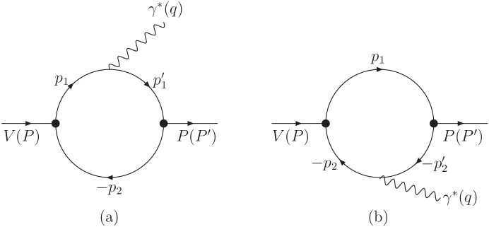
Figure 3: Feynman diagram for $V\to P\gamma^{*}$ process where $P$ in the parenthesis denotes the momentum of initial meson and $P^{\prime}$ denotes the momentum of final meson.

To the lowest order approximation, the $V\to P\gamma^{*}$ transition is depicted in Fig. 3. The amplitude $\Gamma_{\mu}$ is given by a one-loop momentum integral

$$\Gamma_{\mu}=-iee_{q}N_{c}\int\frac{d^{4}p_{1}}{(2\pi)^{4}}\Bigg{\{}\frac{H_{V}H_{P}^{\prime}}{N_{1}N_{2}N_{1}^{\prime}}S^{a}_{\mu\nu}+\frac{H_{V}H_{P}^{\prime}}{N_{1}N_{2}N_{2}^{\prime}}S^{b}_{\mu\nu}\Bigg{\}}\epsilon^{\nu},$$ (26)

where

$$S^{a}_{\mu\nu} = {\rm Tr}\Big{[}\Big{(}\gamma_{\nu}-\frac{1}{W_{V}}(p_{1}-p_{2})_{\nu}\Big{)}(-\not\!p_{2}+m)\gamma_{5}(\not\!p_{1}^{~{}\prime}+m)\gamma_{\mu}(\not\!p_{1}+m)\Big{]},$$

$$S^{b}_{\mu\nu} = {\rm Tr}\Big{[}\Big{(}\gamma_{\nu}-\frac{1}{W_{V}}(p_{1}-p_{2})_{\nu}\Big{)}(-\not\!p_{2}+m)\gamma_{\mu}(-\not\!p_{2}^{~{}\prime}+m)\gamma_{5}(\not\!p_{1}+m)\Big{]},$$ (27)

and

$$N_{1}^{\prime}=p_{1}^{\prime 2}-m^{2}+i\epsilon;\qquad\qquad N_{2}^{\prime}=p_{2}^{\prime 2}-m^{2}+i\epsilon.$$ (28)

The first and second terms in Eq. (26) are arising from diagram (a) and (b) of Fig. 3, respectively. We have used the momentum relations: $P=p_{1}+p_{2}$, $P^{\prime}=p^{\prime}_{1}+p_{2}^{\prime}$, $q=P-P^{\prime}$; $p_{2}=p_{2}^{\prime}$ for diagram Fig. 3(a); $p_{1}=p_{1}^{\prime}$ for diagram Fig. 3(b). It is easy to find that $S^{a}_{\mu\nu}=S^{b}_{\mu\nu}$.

The momentum integral of Eq. (26) are performed analogous to the case of $P\to\gamma\gamma^{*}$. The contour integrals are closed in the upper $p_{1}^{-}$ half-plane for the first term in Eq. (26) which corresponds to putting antiquark on the mass-shell; and in the lower half-plane for the second term which corresponds to putting quark on the mass-shell. For the first term, it leads to the replacements

$$N_{1}^{(\prime)} \to \hat{N}_{1}^{(\prime)}=x_{1}\big{(}M^{(\prime)2}-M_{0}^{(\prime)2}\big{)},$$

$$\int\frac{d^{4}p_{1}}{(2\pi)^{4}}\frac{H_{V}H_{P}^{\prime}}{N_{1}N_{2}N_{1}^{\prime}} \to -i\pi\int\frac{dx_{2}d^{2}p_{\bot}}{(2\pi)^{4}}\frac{h_{V}h_{P}^{\prime}}{x_{2}\hat{N}_{1}\hat{N}_{1}^{\prime}}$$ (29)

In order to preserve the covariance of the decay amplitude, we also need the replacements

$$p_{1}^{\alpha} \to x_{1}P^{\alpha}-q^{\alpha}\frac{p_{\bot}\cdot q_{\bot}}{q^{2}},\qquad\qquad p_{1}^{\alpha}p_{1}^{\beta}\to-g^{\alpha\beta}\left(p_{\bot}^{2}+\frac{(p_{\bot}\cdot q_{\bot})^{2}}{q^{2}}\right).$$ (30)

The similar treatments can be done for the second term. After using the above replacements and Eq. (6), we obtain the formulae for the form factor $V(q^{2})$ as

$$V(q^{2})= \frac{e_{q}}{8\pi^{3}}\int dx_{2}d^{2}p_{\bot}\frac{\phi_{V}(x_{2},p_{\bot})\phi^{\prime}_{P}(x_{2},p^{\prime}_{\bot})}{x_{1}x_{2}M_{0}M_{0}^{\prime}}\left\{m-\frac{2}{w_{V}}\left(p_{\bot}^{2}+\frac{(p_{\bot}\cdot q_{\bot})^{2}}{q^{2}}\right)\right\}.$$ (31)

The rate for $V\to P\gamma$ is

$$\Gamma(V\to P\gamma)=\frac{1}{3}\frac{(M_{V}^{2}-M_{P}^{2})^{3}}{32\pi M_{V}^{3}}(4\pi\alpha)|V(0)|^{2}.$$ (32)

III non-relativistic approximation and perturbative QCD

It is well-known that the system of the heavy quarkonium can be treated non-relativistically QR . A relativistic invariant theory, light-front QCD in our case, should reproduce the previous results in the non-relativistic approximations. Here, we will explore the non-relativistic approximations of the light-front QCD. It is similar to the studies of heavy quark limit for heavy meson CCH1 within the light-front approach. In addition to it, the light-front QCD is related to perturbative QCD at the large momentum transfers, such as in $P\to\gamma\gamma$ process. Both of them show the different aspects of light-front QCD.

At first, we discuss the non-relativistic approximations of the light-front approach. In the rest frame of the heavy quarkonium, the momenta of quark and antiquark are dominated by their rest mass $m\gg\Lambda_{\rm QCD}$ ($\Lambda_{\rm QCD}$ is the hadronic scale). The momentum fractions $x_{1},x_{2}$ are peaked around $\frac{1}{2}$, and $x_{2}-\frac{1}{2}$ is of order $\Lambda_{\rm QCD}/m$. In NRQCD, the velocity of heavy quark is chosen as the expansion parameter. Neglecting the terms suppressed by $1/m$, the invariant mass $M_{0}$ and $p_{z}$ can be approximated as

$$M_{0}\cong 2m\cong M,\qquad\qquad p_{z}=(x_{2}-\frac{1}{2})M_{0}\sim\Lambda_{\rm QCD}.$$ (33)

Compared with $m$, we have neglected the transverse momentum $p_{\bot}$ because it is of the order of $\Lambda_{\rm QCD}$. Thus, the magnitude of the relative momentum $\vec{p}$ will be much smaller than $m$, i.e., $|\vec{p}|\sim\Lambda_{\rm QCD}$, which constitutes the basis of the non-relativistic treatment.

Under the non-relativistic approximations, the dependence of the hadron wave function on $x_{2}$ is replaced by its dependence on $p_{z}$ since $M_{0}\cong M$ is a constant. In this way, the hadron wave function will depend on the relative momentum $\vec{p}$ only, in other words, it can be represented by $\psi(\vec{p})$. The relation between the non-relativistic function $\psi(\vec{p})$ and the relativistic one $\phi(x_{2},p_{\bot})$ can be established as follows. From Eq. (2), we obtain

$$dp_{z}\cong M~{}dx_{2},\qquad\qquad d^{3}p=M~{}dx_{2}d^{2}p_{\bot},$$ (34)

As uausl, the function of $\psi(\vec{p})$ is normalized as

$$\int\frac{d^{3}p}{(2\pi)^{3}}|\psi(\vec{p})|^{2}=1.$$ (35)

Comparing Eqs. (34) and (35) with Eq. (8), it is straightforward to derive a relation

$$\phi(x_{2},p_{\bot})\doteq\sqrt{2M}\psi(\vec{p}).$$ (36)

Note that the above relation is valid within the non-relativistic approximation and is not correct in the general case.

The hadron wave function in the coordinate space $\Psi(\vec{r})$ is obtained by using the Fourier transformation

$$\Psi(\vec{r})=\int\frac{d^{3}p}{(2\pi)^{3}}~{}\psi(\vec{p})~{}e^{i\vec{p}\cdot\vec{r}}.$$ (37)

At the origin $\vec{r}=0$, $\Psi(0)=\int\frac{d^{3}p}{(2\pi)^{3}}~{}\psi(\vec{p})$ is an important parameter which gives the magnitude of quark-antiquark coupling to the quarkonium. In the non-relativistic approximations, one can safely neglect $\vec{p}$ compared to $m$. For example,

$$\sqrt{m^{2}+p_{\bot}^{2}}\to m,~{}~{}~{}x_{2}-\frac{1}{2}\to 0.$$ (38)

After these approximations, we can rewrite the decay constants Eqs. (12) and (14) as

$$f_{P}\doteq 2\sqrt{N_{c}}\frac{\Psi_{P}(0)}{\sqrt{M_{P}}},\qquad\qquad f_{V}\doteq 2\sqrt{N_{c}}\frac{\Psi_{V}(0)}{\sqrt{M_{V}}}.$$ (39)

Thus,

$$\frac{f_{P}^{2}}{f_{V}^{2}}=\frac{M_{V}}{M_{P}}\frac{|\Psi_{P}(0)|^{2}}{|\Psi_{V}(0)|^{2}}.$$ (40)

This is just the so-called Van Royen-Weisskopf formula RW . Since the differences between vector and pseudoscalar vectors arise from the higher order in $1/m$, these differences vanish in the limit $m\to\infty$, thus $M_{V}=M_{P}=2m$, $\Psi_{V}(\vec{p})=\Psi_{P}(\vec{p})$. The ratio of decay constants is equal to 1 in the limit.

For the form factor $V(0)$ of $V\to P\gamma$ process, Eq. (31)can be reduced to

$$V(0)\doteq e_{q}\int\frac{d^{3}\vec{p}}{(2\pi)^{3}}\frac{2\sqrt{M_{P}M_{V}}}{M_{V}}\frac{\Psi_{V}(\vec{p})\Psi_{P}(\vec{p})}{m},$$ (41)

Similarly, in the non-relativistic limit $m\to\infty$, the form factor $V(0)$ can be further written in a simple form as

$$V(0)=2e_{q}/m.$$ (42)

Thus $V(0)$ is a constant, independent of $\Psi(0)$ because of the normalization condition of $\Psi(\vec{p})$. The physical picture is: the heavy quark and antiquark in the initial and final quarkonium are in the same momentum configuration at $q^{2}=0$ point. It is analogous to the meson system with a single heavy quark that the Isgur-Wise function is normalized to 1 at the zero-recoil point in the infinite heavy quark mass limit. From Eqs. (32) and (42), the rate for the $V\to P\gamma$ process is reduced into

$$\Gamma(V\to P\gamma)=\frac{16}{3}\alpha e_{q}^{2}\frac{k_{\gamma}^{3}}{M_{V}^{2}}.$$ (43)

where $k_{\gamma}=(M_{V}^{2}-M_{P}^{2})/2M_{V}$ is the energy of the photon. This is the leading order result of Eq. (37) in BJV .

Next, we discuss that the pQCD is applicable in $P\to\gamma\gamma$ process. In the rest frame of the heavy quarkonium, the total energy is $2m\gg\Lambda_{\rm QCD}$. Each final photon contains high energy of $m$ and moves in the opposite light-front direction. When the high energy photon hits on one nearly rest constituent of the quarkonium, it causes a large virtuality of the order of $m^{2}$. In particular, the virtuality of the internal quark is about $2m^{2}$ from Eqs. (II.3) and (II.3). The transverse momentum in the propagator of the virtual quark can be neglected. Up to leading order in $\Lambda_{\rm QCD}/m$, the transition form factor $F_{P\gamma}(0)$ is represented by

$$F_{P\gamma}(0) = e_{q}^{2}\sqrt{2N_{c}}\int\frac{dx_{2}d^{2}p_{\bot}}{(2\pi)^{3}}\phi(x_{2},p_{\bot})~{}T_{H}(x_{2})$$ (44)

$$\propto \int dx_{2}~{}\Phi(x_{2})T_{H}(x_{2}).$$

where $\Phi(x_{2})$ is the hadron distribution amplitude obtained from wave function by integral over the transverse momentum, and $T_{H}(x_{2})$ is the hard scattering kernel from the subprocess of $q\bar{q}\to\gamma\gamma$.

The hard scattering kernel depends on momentum fraction $x_{2}$ when the loop corrections are taken into account. But, at tree level, the hard scattering kernel is

$$T_{H}=\frac{1}{m^{2}},$$ (45)

It is not only independent of transverse momentum $p_{\bot}$ but also of longitudinal fraction $x_{2}$. We thus have a further result

$$F_{P\gamma}(0)=e_{q}^{2}\frac{f_{P}}{m^{2}}.$$ (46)

This equation means that the form factor $F_{P\gamma}(0)$ is proportional to the decay constant $f_{P}$ in leading order $\Lambda_{\rm QCD}/m$ and leading order of strong coupling constant $\alpha_{s}$. After combining Eqs. (15), (24), (39), and (46), we finally obtain the decay rates for processes of $V\to e^{+}e^{-}$ and $P\to\gamma\gamma$ as

$$\Gamma(V\to e^{+}e^{-}) = {16\over{3}}N_{c}\pi\alpha^{2}c_{V}\frac{|\Psi_{V}(0)|^{2}}{M_{V}^{2}},$$

$$\Gamma(P\to\gamma\gamma) = 16N_{c}\pi\alpha^{2}e_{q}^{4}\frac{|\Psi_{P}(0)|^{2}}{M_{P}^{2}}.$$ (47)

These results are the same as ones in Table III in the non-relativistic quark-potential model KMRR .

IV Numerical results and discussions

In order to obtain the numerical results, the crucial thing is to determine the momentum distribution amplitude $\phi(x_{2},p_{\bot})$. One wave function that has been often used in the literature for mesons is the Gaussian-type

$$\phi(x_{2},p_{\bot})=N\sqrt{\frac{dp_{z}}{dx_{2}}}~{}{\rm exp}\left(-\frac{p_{\bot}^{2}+p_{z}^{2}}{2\beta^{2}}\right),$$ (48)

with $N=4(\pi/{\beta^{2}})^{3/4}$ and

$$\frac{dp_{z}}{dx_{2}}=\frac{e^{2}}{x_{1}x_{2}M_{0}}.$$ (49)

The required input parameters include quark mass: $m_{c}$ for c quark and $m_{b}$ for b quark; a hadronic scale parameter $\beta$ for $\eta_{c(b)}$ and $J/\psi(\Upsilon)$. The quark mass entered into our analysis is the constituent mass. For light quarks (u and d), the constituent mass which several hundred MeV, is quite bigger than the current one which is only several MeV obtained from the chiral perturbation theory. While for the heavy quarks, the difference between them is small. From PDG PDG06 , the current masses are $1~{}{\rm GeV}\leq m_{c}\leq 1.4~{}{\rm GeV}$ and $4~{}{\rm GeV}\leq m_{b}\leq 4.5~{}{\rm GeV}$ in the ${\rm\overline{MS}}$ renormalization scheme. For our purpose, we will choose heavy quark constituent masses as

$$m_{c}=1.2~{}{\rm GeV},\qquad\qquad m_{b}=4.3~{}{\rm GeV}.$$ (50)

Our choices are smaller than the parameters given in CCH2 , but they are consistent within the error of one $\Lambda_{\rm QCD}$. For the meson mass, $M_{\eta_{c}}=2.980~{}{\rm GeV}$, $M_{J/\psi}=3.097~{}{\rm GeV}$ and $M_{\Upsilon}=9.460~{}{\rm GeV}$ PDG06 . The mass of $\eta_{b}$ is still unknown and it is parameterized as $\Delta m=M_{\Upsilon}-M_{\eta_{b}}$. From the references in ALEPH , the range of $\Delta m$ is $\Delta m=30-150$ MeV.

After fixing the quark and meson masses, the remained thing is to determine the parameters $\beta$. For the vector meson, $\beta_{V}$ is extracted from the decay constant $f_{V}$ which is obtained directly from the process $V\to e^{+}e^{-}$ by Eq. (15). For the pseudoscalar meson $\eta_{c}$, $\beta_{\eta_{c}}$ is extracted from the decay constant $f_{\eta_{c}}$ which is obtained from the process $B\to\eta_{c}K$.

For the $c\bar{c}$ charmonium system, there are some experiment data which provides a place to test the applicability of the Gaussian-type wave function to the heavy quarkonium. From $J/\psi\to e^{+}e^{-}$, we obtain $f_{J/\psi}=416\pm 6$ MeV, and extract $\beta_{J/\psi}=0.639\pm 0.006$ GeV. From $B\to\eta_{c}K$, one obtains $f_{\eta_{c}}=335\pm 75$ MeV fetac , and we extract $\beta_{\eta_{c}}=0.652^{+0.165}_{-0.143}$ GeV. It is apparent that the dominant errors in the following calculations will be derived from the uncertainty of $f_{\eta_{c}}$. By using the above parameters, we give the numerical results for $\eta_{c}\to\gamma\gamma$: $Br(\eta_{c}\to\gamma\gamma)=(1.78\sim 3.05)\times 10^{-4}$ and for $J/\psi\to\eta_{c}\gamma$: $Br(J/\psi\to\eta_{c}\gamma)=(2.38\sim 2.84)\times 10^{-2}$. The experimental data are $Br(\eta_{c}\to\gamma\gamma)=(2.8\pm 0.9)\times 10^{-4}$ and $Br(J/\psi\to\eta_{c}\gamma)=(1.3\pm 0.4)\times 10^{-2}$. Obviously the former fits experiment very well but the latter does not. This inconsistency still exists even we adjust the quark mass $m_{c}$ in the range $1\sim 1.4~{}{\rm GeV}$.

One may consider a power law wave function similar to the one employed in Ref. BS to fit the data, however, the Gaussian-type wave function has been used widely in the phenomenal analyses which related to meson. Thus we modify the Gaussian-type wave function by just multiplying a factor $(x_{1}x_{2})^{n}$

$$\tilde{\phi}(x_{2},p_{\perp})=\tilde{N}(x_{1}x_{2})^{n}\sqrt{\frac{dp_{z}}{dx_{2}}}~{}{\rm exp}\left(-\frac{p_{\bot}^{2}+p_{z}^{2}}{2\tilde{\beta}^{2}}\right).$$ (51)

The curve which $x_{2}$ is peaked around ${1\over{2}}$ will be sharped or dulled if $n>0$ or $n<0$, respectively. In the non-relativistic limit, Eq. (38) reveals that the curve is near to a delta function $\delta(x_{2}-{1\over{2}})$. Therefore the case of $n>0$ seems suitable for the heavy quarkonium. In fact, if $n=5$ and $m_{c}=1.2$ GeV, we can extract $\tilde{\beta}_{J/\psi}=0.786\pm 0.008$ GeV and $\tilde{\beta}_{\eta_{c}}=0.807^{+0.273}_{-0.211}$ GeV. The numerical results $Br(\eta_{c}\to\gamma\gamma)=(1.56\sim 2.06)\times 10^{-4}$ and $Br(J/\psi\to\eta_{c}\gamma)=(1.62\sim 2.41)\times 10^{-2}$ are both consistent with the experimental data. Thus there is a deduction that, for heavy quarkonium, the momentum fraction $x_{2}$ is more centered on ${1\over{2}}$ than one is in the Gaussian-type wave function. We show the $x$-dependent behaviors of these two types of wave functions in Fig. 4 and the numerical results in Table 1.

Figure 4: The $x$-dependent behaviors of $\phi$ (dash line) and $\tilde{\phi}$ (solid line, n=5) at $p^{2}_{\perp}=0.1$ GeV².

Table 1: The comparisons between the experimental data and theory predictions for charmonium decays.

	$Br(\eta_{c}\to\gamma\gamma)$	$Br(J/\psi\to\eta_{c}\gamma)$
experiment data	$(2.8\pm 0.9)\times 10^{-4}$	$(1.3\pm 0.4)\%$
this work $(\phi)$	$(1.78\sim 3.05)\times 10^{-4}$	$(2.38\sim 2.84)\%$
this work $(\tilde{\phi})$	$(1.56\sim 2.06)\times 10^{-4}$	$(1.62\sim 2.41)\%$

For the $b\bar{b}$ bottomonium system, the experimental data are relatively less. From $\Upsilon(1S)\to e^{+}e^{-}$, we obtain $f_{\Upsilon}=708\pm 8$ MeV, then extract $\beta_{\Upsilon}=1.323\pm 0.010$ GeV and $\tilde{\beta}_{\Upsilon}=1.463\pm 0.012$ GeV. However, $\eta_{b}$ meson hasn’t been observed in experiment. It is impossible to determine the decay constant $f_{\eta_{b}}$ from the experiment. As had been discussed, the relation $f_{\eta_{b}}=f_{\Upsilon}$ is hold in the non-relativistic limit. Since the corrections to this relation are suppressed by $\Lambda_{\rm QCD}/m_{b}$, it may be reasonable to use it to determine the parameter $\beta_{\eta_{b}}(\tilde{\beta}_{\eta_{b}})$. Therefore we obtain $\beta_{\eta_{b}}=1.433\pm 0.014$ and $\tilde{\beta}_{\eta_{b}}=1.607\pm 0.018$ GeV. For obtaining the decay widths $\Gamma(\eta_{b}\to\gamma\gamma)$ and $\Gamma(\Upsilon\to\eta_{b}\gamma)$, we must be aware of the value of $\Delta m$. However, the sensitivities of these two decay widths to $\Delta m$ are quite different. On the one hand, $\Gamma(\eta_{b}\to\gamma\gamma)$ is insensitive to $\Delta m$ because $M_{\eta_{b}}\gg\Delta m$ (see Eq. (24)). On the other hand, $\Gamma(\Upsilon\to\eta_{b}\gamma)$ is very sensitive to $\Delta m$ because it is proportional to $(\Delta m)^{3}$ (see Eq. (32)). Thus here we list the values of $\Gamma(\eta_{b}\to\gamma\gamma)$ for $\Delta m=0.09\pm 0.06$ GeV and $\Gamma(\Upsilon\to\eta_{b}\gamma)$ for $\Delta m=0.09$ GeV in Table 2. The dependences of $\Upsilon\to\eta_{b}\gamma$ on $\Delta m$ are also shown in Fig. 5.

Table 2: The comparisons among the several theory predictions for bottomonium decays.

	$\Gamma(\eta_{b}\to\gamma\gamma)$ (eV)	$\Gamma(\Upsilon\to\eta_{b}\gamma)$ (eV)
this work $(\phi)$	$453\pm 17$	$33.2\pm 0.1$
this work $(\tilde{\phi})$	$422\pm 15$	$31.5\pm 0.1$
used in ALEPH	$557\pm 85$	-
NRQCD NRQCD1 $\cal{O}(\alpha_{\mathrm{s}})$	$460$	-
potential model potential	$466\pm 101$	-

Figure 5: The dependences of $\Gamma(\Upsilon\to\eta_{b}\gamma)$ on $\Delta m=M_{\Upsilon}-M_{\eta_{b}}$.

For the numerical results, some comments are in orders:

(1) The decay constant for $\eta_{c}$ is $f_{\eta_{c}}=335\pm 75$ MeV fetac , and we obtain

$$\left(\frac{f_{\eta_{c}}}{f_{J/\psi}}\right)^{2}\approx 0.65\pm 0.31.$$ (52)

The difference between the pseudoscalar and vector meson in light-front approach comes from power suppressed terms: the transverse momentum $p_{\perp}$, $x_{2}-\frac{1}{2}$ and the wave function $\phi(x,p_{\perp})$. The deviation of the results from 1 shows that $\Lambda_{\rm QCD}/m_{c}\sim 30\%$ corrections cannot be neglected.

(2) For the M1 transition $J/\psi\to\eta_{c}\gamma$, the leading order prediction from Eq. (43) for the branching ratio is $4.2\%$ which is about a factor of 3 larger than the experimental data. This means that the next-to-leading order $\Lambda_{\rm QCD}/m_{c}$ corrections are so substantial that they must be included in the calculations.

(3) For the decay width $\Gamma(\eta_{b}\to\gamma\gamma)$, it is insensitive to the variations of $\Delta m$ but proportional to $f_{\eta_{b}}^{2}$. Thus an adjustment of $f_{\eta_{b}}$ by $10\%$ will correspond to a variation of the theory prediction by about $20\%$. So far, $(f_{\eta_{b}}/f_{\Upsilon})^{2}=1$ is our assumption and $0.99\pm 0.04$ in HK and $1.16\pm 0.06$ in AM . After considering these uncertainties, our prediction may be consistent with previous results listed in ALEPH ; NRQCD1 ; potential .

V Conclusions

In this article we have studied the decay constants, two-photon annihilation $P\to\gamma\gamma$ and magnetic dipole transition $V\to P\gamma$ processes for the ground-state heavy quarkonium within the covariant light-front approach. The phenomenological parameters and wave functions are determined from the experiment. The predictions agree with the measured data within the theoretical and experimental errors. The quark mass we use is very close to the current mass which is different from the choices in non-relativistic quark model. The difference between the $J/\psi$ and $\eta_{c}$ decay constants and the study in $J/\psi\to\eta_{c}\gamma$ both show that the power corrections from wave functions and transverse momentum effects are important. In order to make a better fit to the experimental data, we adjust the longitudinal momentum fraction of the wave function to center around $1/2$ further. We also give a numerical prediction for $\eta_{b}\to\gamma\gamma$ and $\Upsilon\to\eta_{b}\gamma$. The branching ratio for $\Upsilon\to\eta_{b}\gamma$ is too small to be observed. $\eta_{b}\to\gamma\gamma$ may be a good process to determine $\eta_{b}$ and its mass. The QCD corrections are neglected in this study, including them will slightly change the wave function inputs but does not change our conclusions.

The light-front approach shows different aspects of QCD. Under the non-relativistic approximations, the light-front approach reproduces the results in the non-relativistic quark-potential model. For $P\to\gamma\gamma$ where two final photons are on the opposite light-front, the process is perturbative dominated and the light-front approach reduces to the model-independent pQCD. The light-front method unifies the perturbative and non-perturbative QCD into the same framework.

We have considered s-wave heavy quarkonium in the light-front approach only, the applications to other quantities and higher resonances are in progress. One interesting thing may be to explore the light-front approach in NRQCD (or pNRQCD). This will provide an alternative non-perturbative method to calculate the hadronic matrix elements defined in NRQCD.

Acknowledgments
We thank Hai-Yang Cheng and Chun-Khiang Chua for many valuable discussions. We also wish to thank the National Center for Theoretical Sciences (South) for its hospitality during our summer visits where this work started. This work was supported in part by the National Science Council of R.O.C. under Grant No. NSC94-2112-M-017-004.

References

- (1) C. Quigg and J. L. Rosner, Phys. Rept. 56, 167-235 (1979).
- (2) N. Brambilla et al., CERN-2005-005, [hep-ph/0412158].
- (3) S. J. Brodsky, H. C. Pauli and S. S. Pinsky, Phys. Rept. 301, 299 (1998).
- (4) M. V. Terent’ev, Sov. J. Phys. 24, 106 (1976); V. B. Berestetsky and M. V. Terent’ev, ibid.24, 547 (1976); ibid. 25, 347 (1977).
- (5) W. Jaus, Phys. Rev. D41, 3394 (1990); ibid. 44, 2851 (1991).
- (6) H. Y. Cheng, C. Y. Cheung and C. W. Hwang, Phys. Rev. D 55, 1159 (1997).
- (7) W. Jaus, Phys. Rev. D60, 054026 (1999).
- (8) H. Y. Cheng, C. K. Chua and C. W. Hwang, Phys. Rev. D 69, 074025 (2004).
- (9) C. W. Hwang, Phys. Rev. D64, 034011 (2001).
- (10) W. Kwong, P. B. Mackenzie, R. Rosenfeld and J. L. Rosner, Phys. Rev. D37, 3210 (1988).
- (11) E. S. Ackleh, T. Barnes, Phys. Rev. D45, 232 (1992).
- (12) N. Brambila, Y. Jia and A. Vairo, Phys. Rev. D73, 054005 (2006).
- (13) J. J. Dudek, R. G. Edwards and D. G. Richards, Phys. Rev. D73, 074507 (2006).
- (14) ALEPH Collaboration, Phys. Lett. B 530 56-66 (2002).
- (15) H. C. Pauli and S. J. Brodsky, Phys. Rev. D32, 1993; 2001 (1985).
- (16) A. C. Tang, S. J. Brodsky, and H. C. Pauli, Phys. Rev. D44, 1842 (1991).
- (17) M. Kaluza and H. C. Pauli, Phys. Rev. D45, 2968 (1992).
- (18) M. Kaluza and H.-J. Pirner, Phys. Rev. D47, 1620 (1993).
- (19) R. J. Perry, A. Harindranath, and K. G. Wilson, Phys. Rev. Lett. 65, 2959 (1990).
- (20) R. J. Perry and A. Harindranath, Phys. Rev. D43, 4051 (1991).
- (21) S. Głazek, A. Harindranath, S. Pinsky, J. Shigemitsu, and K. G. Wilson, Phys. Rev. D47, 1599 (1993).
- (22) I. Tamm. J. Phys. (USSR) 9, 449 (1949).
- (23) S. M. Dancoff, Phys. Rev. 78, 382 (1950).
- (24) T. Eller, H. C. Pauli, and S. J. Brodsky, Phys. Rev. D35, 1493 (1987).
- (25) M. Neubert and B. Stech, Adv. Ser. Direct. High Energy Phys. 15, 294-344 (1998).
- (26) R. Van Royen and V. F. Weisskopf, Nuovo Cim. 50, 617 (1967); .51, 583E (1967).
- (27) Particle Data Group 2006, W.-M. Yao et al., Journal of Physics G 33, 1 (2006).
- (28) K. W. Edwards et al., CLEO Collaboration, Phys. Rev. Lett. 86, 30-40 (2001).
- (29) S. J. Brodsky and F. Schlumpf, Phys. Lett. B 329, 111-116, (1994).
- (30) G. A. Schuler, F. A. Berends, and R. van Gulik, Nucl. Phys. B 523, 423-438 (1998).
- (31) N. Fabiano, Eur. Phys. J. C 26, 441-444 (2003).
- (32) D. S. Hwang and G. H. Kim, Z. Phys. C 76, 107-110 (1997).
- (33) M. R. Ahmady and R. R. Mendel, Phys. Rev. D51, 141 (1995).