Abstract

In the dynamical gauge-Higgs unification the 4D Higgs field is unified with gauge fields and the electroweak symmetry is dynamically broken by the Hosotani mechanism. Interesting phenomenology is obtained in the Randall-Sundrum warped spacetime. (i) The Higgs boson mass is predicted at the LHC energies. (ii) The hierarchy in the fermion mass spectrum is naturally explained. (iii) Tiny violation of the universality in the charged current interactions is predicted. (iv) Yukawa couplings of quarks and leptons are suppressed compared with those in the standard model. (v) $WWH$, $ZZH$ couplings are suppressed compared with those in the standard model.

OU-HET 566/2006

October 19, 2006

1 Introduction

In the gauge-Higgs unification 4D Higgs scalar fields are unified with 4D gauge fields within the framework of higher dimensional gauge theory. Low energy modes of extra-dimensional components of gauge potentials are 4D Higgs fields. The scenario works remarkably well when the extra-dimensional space is non-simply-connected.[1, 2] There arise Yang-Mills AB (Aharonov-Bohm) phases along the extra dimension, whose fluctuations in four dimensions are nothing but the 4D Higgs fields. The most notable feature is that quantum dynamics generate non-trivial, finite effective potential for the Higgs fields, inducing dynamical gauge symmetry breaking and generating finite masses for the Higgs fields at the same time. Even though the theory is non-renormalizable, many properties of the Higgs fields can be deduced irrespective of unknown dynamics at the cutoff scale. The Higgs boson mass turns out to be much smaller than the Kaluza-Klein mass scale. This is contrasted to the earlier proposal of the gauge-Higgs unification based on the ad hoc symmetry ansatz.[3, 4]

In the last ten years the scenario of the gauge-Higgs unification has been applied to the electroweak interactions and grand unified theories with the aid of orbifolds as extra dimensions.[5]-[21] In this article we focus on applications to the electroweak interactions where, besides the Higgs boson mass, many illuminating predictions are made for LHC and linear colliders.

To achieve the gauge-Higgs unification in the electroweak interactions, there are a few requirements to be fulfilled. First of all, the electroweak gauge symmetry is $SU(2)_{L}\times U(1)_{Y}$ which breaks down to $U(1)_{\rm EM}$ triggered by non-vanishing VEV of an $SU(2)_{L}$ doublet Higgs field. In order for the 4D Higgs field be a part of gauge potentials the original gauge group must be larger than $SU(2)_{L}\times U(1)$. Secondly, fermion content must be chiral. The second requirement is restrictive, as fermions in higher dimensions tend to lead to vectorlike theory in the effective 4D theory at low energies, unless the extra-dimensional space has nontrivial topology or there exists nonvanishing flux in the extra dimensions. These requirements can be naturally and easily fulfilled when the extra dimensional space is an orbifold.

1.1 Gauge theory on an orbifold

Consider $S^{1}$ with a coordinate $y$ where $y$ and $y+2\pi R$ are identified. Further we identify $y$ and $-y$, which gives an orbifold $S^{1}/Z_{2}$. There appear two fixed points under parity; $y_{0}=0$ and $y_{1}=\pi R$. Let us analyse gauge theory on $M^{4}\times(S^{1}/Z_{2})$, which is first defined on a covering space $M^{5}$, supplemented with restrictions appropriate to preserve the nature of $S^{1}/Z_{2}$. Although $y_{j}+y$ and $y_{j}-y$ represent the same physical point, gauge potentials need not be the same. They may differ from each other up to a gauge transformation. The orbifold structure is respected if

$$\begin{pmatrix}A_{\mu}\cr A_{y}\end{pmatrix}(x,y_{j}-y)=P_{j}\begin{pmatrix}A_{\mu}\cr-A_{y}\end{pmatrix}(x,y_{j}+y)P_{j}^{\dagger}$$ (1)

where $P_{j}$ is an element of the gauge group satisfying $P_{j}^{2}=I$. Similarly for fermions in the spinor representation in an $SU(N)$ group or in the vector representation in an $SO(N)$ group

$$\psi(x,y_{j}-y)=\pm P_{j}\gamma^{5}\psi(x,y_{j}+y)~{}~{}.$$ (2)

If $P_{j}\not{\kern-2.0pt\propto}~{}I$, the gauge symmetry $G$ apparently breaks down to a smaller subugroup $H_{{\rm BC}}$. $\{P_{0},P_{1}\}$ defines the symmetry of boundary condition. $H_{{\rm BC}}$ is not necessarily the physical symmetry $H_{\rm phys}$ which survives at the end. $H_{\rm phys}$ can be either smaller or larger than $H_{{\rm BC}}$. Put it differently, two distinct sets of boundary conditions, $\{P_{0},P_{1}\}$ and $\{P_{0}^{\prime},P_{1}^{\prime}\}$ can be equivalent to each other in physics content. All of these are due to dynamics of Yang-Mills AB phases. It is called the Hosotani mechanism.[1, 2, 10] In the application to the electroweak interactions we would like to have $H_{{\rm BC}}=SU(2)_{L}\times U(1)_{Y}$ and $H_{\rm phys}=U(1)_{\rm EM}$.

In the $SU(3)$ model, $P_{0}=P_{1}={\rm diag}~{}(-1,-1,1)$ gives $H_{{\rm BC}}=SU(2)\times U(1)$. Zero modes exist for the $H_{{\rm BC}}$ part of $A_{\mu}$ and for the $G/H_{{\rm BC}}$ part of $A_{y}$ which forms an $SU(2)$ doublet and idetified with the 4D Higgs field. Although this model gives an incorrect Weinberg angle, it gives a nice working ground to investigate physics of the $W$ boson and fermions. Another model of interest is the $SO(5)\times U(1)_{B-L}$ model proposed by Agashe et al.[16] For the $SO(5)$ part we take $P_{0}=P_{1}={\rm diag}~{}(-1,-1,-1,-1,1)$, which gives $H_{{\rm BC}}^{\prime}=SO(4)\times U(1)_{B-L}=SU(2)_{L}\times SU(2)_{R}\times U(1)_{B-L}$. With additional dynamics on the one of the branes at $y=0$, the symmetry of boundary conditions is reduced to $H_{{\rm BC}}=SU(2)_{L}\times U(1)_{Y}$. Zero modes of $A_{y}$ are located at

$$A_{y}\sim\begin{pmatrix}&&&&-i\phi_{1}\cr&&&&-i\phi_{2}\cr&&&&-i\phi_{3}\cr&&&&-i\phi_{4}\cr i\phi_{1}&i\phi_{2}&i\phi_{3}&i\phi_{4}&\end{pmatrix}~{}~{},~{}~{}\Phi=\begin{pmatrix}\phi_{1}+i\phi_{2}\cr\phi_{4}-i\phi_{3}\end{pmatrix}~{}~{}.$$ (3)

$\Phi$ is the 4D Higgs doublet in the standard model. We note that with the given $\{P_{0},P_{1}\}$, $A_{M}$ becomes periodic; $A_{M}(x,y+2\pi R)=A_{M}(x,y)$.

1.2 Yang-Mills AB phase $\theta_{H}$

The zero modes of $A_{y}$ lead to non-Abelian generalization of the Aharonov-Bohm phases (Yang-Mills AB phases). The configuration gives vanishing field strengths $F_{MN}=0$, but gives nontrivial phases

$$e^{i\Theta_{H}/2}=P\exp\bigg{\{}ig_{A}\int_{0}^{\pi R}dy\,A_{y}\bigg{\}}~{}~{}.$$ (4)

The spectrum of gauge fields and fermions depends on $\Theta_{H}$. The phase $\Theta_{H}$ is a physical quantity. As seen in eq.  (3), the 4D Higgs fields are four-dimensional fluctuations of the Yang-Mills AB phases. This property leads to the finiteness of the Higgs boson mass.[1], [5], [22]-[25]

In the $SO(5)\times U(1)_{B-L}$ model one can suppose with the use of the residual $SU(2)_{L}$ symmetry that only the $\phi_{4}$ component of $A_{y}$ is nonvanishing in the vacuum. The Yang-Mills AB phase $\theta_{H}$ is given by

$$\Theta_{H}=\theta_{H}\cdot\Lambda~{}~{}~{},~{}~{}~{}\Lambda=\begin{pmatrix}0\cr&0\cr&&0\cr&&&&-i\cr&&&i\end{pmatrix}$$ (5)

There exist large gauge transformations which shift $\theta_{H}$ by multiples of $2\pi$, while preserving the boundary conditions;

$$\hskip-28.45274ptA_{M}^{\prime}=\Omega A_{M}\Omega^{\dagger}+\frac{i}{g}\Omega\partial_{M}\Omega^{\dagger}~{}~{},~{}~{}\Omega=e^{iny/R\cdot\Lambda}$$ (6)

$$\hskip-28.45274pt\theta_{H}^{\prime}=\theta_{H}+2\pi n~{}~{}.$$ (7)

It is seen that the phase nature of $\theta_{H}$ is a consequence of the large gauge invariance.

2 Difficulties in flat space

Before going into detailed discussions in the Randall-Sundrum warped spacetime, we briefly summarize difficulties one encounters in gauge-Higgs unification in flat spacetime. The value of $\theta_{H}$ is dynamically determined once the matter content is specified. In typical situation the global minimum of the effective potential $V_{\rm eff}(\theta_{H})$ is located either at $\theta_{H}=0$ or at $\theta_{H}=O(1)$. In the former case the gauge symmetry $H_{\rm BC}$ is unbroken, whereas in the latter case the symmetry breaks down to $U(1)_{\rm EM}$.

The $W$ boson mass, $m_{W}$, becomes non-vanishing for $\theta_{H}\not=0$ at the tree level. In flat space

$$m_{W}\sim\frac{|\sin\theta_{H}|}{\pi R}$$ (8)

which implies that the Kaluza-Klein mass scale $M_{KK}$ is too low. Since the 4D Higgs boson corresponds to four-dimensional fluctuations of $\theta_{H}$, its mass arises as radiative corrections. It turns out finite, but is given by

$$m_{H}\sim\sqrt{\frac{\alpha_{W}}{30}}~{}\frac{1}{R}\sim\sqrt{\frac{\alpha_{W}}{30}}~{}\frac{\pi m_{W}}{|\sin\theta_{H}|}$$ (9)

which typically gives too small $m_{H}\sim 10\,$GeV. Of course, $\theta_{H}$ can be small as a result of cancellations among contributions from various matter fields. However, it requires tuning of the matter content. We argue that natural resolution of the problem can be found once the gauge-Higgs unification is achieved in the Randall-Sundrum spacetime.

3 The Randall-Sundrum warped spacetime

The Randall-Sundrum (RS) warped spacetime is given by

$$\hskip-28.45274ptds^{2}=e^{2\sigma(y)}(\eta_{\mu\nu}dx^{\mu}dx^{\nu}-dy^{2})$$ (10)

$$\hskip-28.45274pt\sigma(y+2\pi R)=\sigma(y)=\sigma(-y)~{}~{},$$ (11)

$$\hskip-28.45274pt\sigma(y)=k|y|\quad{\rm for~{}}|y|\leq\pi R~{}~{},$$ (12)

where $\eta_{\mu\nu}={\rm diag}~{}(1,-1,-1,-1)$. It has topology of $S^{1}/Z_{2}$. In the bulk five-dimensional spacetime $0<y<\pi R$, the cosmological constant is given by $-k^{2}$. In other words, the RS spacetime is the 5D anti-de Sitter space sandwiched by the Planck brane (at $y=0$) and the TeV brane (at $y=\pi R$). The warp factor $e^{\pi kR}$ provides natural explanation of the large hierarchy factor $M_{\rm Pl}/m_{W}\sim 10^{17}$, as was originally pointed out by Randall and Sundrum.[26] We examine gauge theory defined on the RS spacetime. Many surprises are hidden there.[19, 21]

The spectrum of various fields in the RS spacetime has been analyzed by many authors.[27, 28] Each field has a Kaluza-Klein tower, which has a spectrum $m_{n}\sim M_{KK}n$ for large $n$ with the Kaluza-Klein mass scale $M_{KK}$given by

$$M_{KK}\sim\frac{\pi k}{e^{\pi kR}-1}=\begin{cases}1/R&\text{as $k\rightarrow 0$,}\cr\pi ke^{-\pi kR}&\text{for $kR>2$.}\end{cases}$$ (13)

It is legitimate to suppose that $k=O(M_{\rm Pl})$. For $kR\sim 12$, $M_{KK}$ comes out in the TeV range. In the RS spacetime, the spectrum is not with an equal spacing for small $n$.

4 $W$ boson and $Z$ boson

As in the flat spacetime, $W$ bosons and $Z$ bosons acquire finite masses as the Yang-Mills AB phase $\theta_{H}$ becomes nonvanishing. In the $SU(3)$ model the eigenstate of the $W$ boson becomes a mixture of $A^{21}_{\mu}$ and $A^{31}_{\mu}$. Its mass is given by

$$m_{W}\sim\sqrt{\frac{2k}{\pi R}}~{}e^{-\pi kR}\Big{|}\sin\frac{\theta_{H}}{2}\Big{|}~{}.$$ (14)

The neutral current sector is not realistic at all.

In the $SO(5)\times U(1)_{B-L}$ model we denote $SO(5)$ gauge fields in the $SU(2)_{L}$, $SU(2)_{R}$, and $SO(5)/SU(2)_{L}\times SU(2)_{R}$ parts by $A^{j_{L}}_{\mu}$, $A^{j_{R}}_{\mu}$, and $A^{\hat{a}}_{\mu}$ ($j=1,2,3$, $a=1,2,3,4$), and $U(1)_{B-L}$ gauge fields by $B_{\mu}$, respectively. The $W$ boson becomes a mixture of $A^{1_{L}}_{\mu}+iA^{2_{L}}_{\mu}$, $A^{1_{R}}_{\mu}+iA^{2_{R}}_{\mu}$, and $A^{\hat{1}}_{\mu}+iA^{\hat{2}}_{\mu}$ with a mass

$$m_{W}\sim\sqrt{\frac{k}{\pi R}}~{}e^{-\pi kR}\big{|}\sin\theta_{H}\big{|}~{}.$$ (15)

The $Z$ boson becomes a mixture of $A^{3_{L}}_{\mu}$, $B_{\mu}$, $A^{3_{R}}_{\mu}$ and $A^{\hat{3}}_{\mu}$ with a mass

$$\hskip-28.45274ptm_{Z}\sim\frac{m_{W}}{\cos\theta_{W}}~{}~{},$$ (16)

$$\hskip-28.45274pt\sin\theta_{W}=\frac{g_{B}}{\sqrt{g_{A}^{2}+2g_{B}^{2}}}=\frac{g_{Y}}{\sqrt{g_{A}^{2}+g_{Y}^{2}}}$$ (17)

where $g_{A}$ and $g_{B}$ are the $SO(5)$ and $U(1)$ gauge coupling constants, respectively. $g_{Y}$ is the weak hypercharge gauge coupling constant.

When $\sin\theta_{H}$ is $O(1)$, or unless $\theta_{H}\ll 1$, the relation (15) implies that $kR\sim 12~{}(6)$ for $k\sim O(M_{\rm Pl})$ ($10^{12}$ GeV). With $kR=12$, $M_{KK}$ turns out $1.8\sim 3.5$ TeV for $\theta_{H}=(0.4\sim 0.2)\pi$.

5 Higgs boson

The 4D Higgs field corresponds to four-dimensional fluctuations of the Yang-Mills AB phase $\theta_{H}$ so that its mass and self-couplings can be obtained from the effective potential for $\theta_{H}$. In the $SO(5)\times U(1)_{B-L}$ model the zero mode of $A_{y}$ is related to the 4D neutral Higgs field $\phi^{0}$ by

$$A_{y}=\sqrt{\frac{k}{2(e^{2\pi kR}-1)}}~{}e^{2ky}~{}\phi^{0}(x)\cdot\Lambda~{}~{}.$$ (18)

The effective potential $V_{{\rm eff}}(\theta_{H})$ at one loop is given by

$$V_{{\rm eff}}(\theta_{H})=\sum\mp\frac{i}{2}\int\frac{d^{4}p}{(2\pi)^{4}}\sum_{n}\ln\Big{\{}p^{2}+m_{n}^{2}(\theta_{H})\Big{\}}~{}~{}.$$ (19)

It is shown that the $\theta_{H}$-dependent part of $V_{{\rm eff}}(\theta_{H})$ is finite, independent of the cutoff scale.[1, 2, 17] In a model with standard matter content it is

$$V_{{\rm eff}}(\theta_{H})\sim\frac{3}{128\pi^{6}}~{}M_{KK}^{4}~{}f(\theta_{H})~{}~{},$$ (20)

where the amplitude of $f(\theta_{H})=f(\theta_{H}+2\pi)$ is $O(1)$ as confirmed in various models.

Suppose that the global minimum of $V_{{\rm eff}}(\theta_{H})$ is located at $\theta_{H}\not=0~{}(mod~{}\pi)$ so that the electroweak symmetry breaks down. By expanding the effective potential around the global minimum one can determine the mass of the Higgs boson and its self-couplings. The mass and quartic coupling are found, in the $SO(5)\times U(1)_{B-L}$ model, to be

$$\hskip-28.45274ptm_{H}\sim\sqrt{\frac{3\alpha_{W}}{32\pi}f^{(2)}(\theta_{H})}~{}\frac{\pi kR}{2}~{}\frac{\sqrt{2}\,m_{W}}{\sin\theta_{H}}~{}~{},$$ (21)

$$\hskip-28.45274pt\lambda\sim\frac{\alpha_{W}^{2}}{16}~{}f^{(4)}(\theta_{H})\bigg{(}\frac{\pi kR}{2}\bigg{)}^{2}~{}~{}.$$ (22)

Notice the presence of the enhancement factor $\pi kR/2\sim 20$, which is absent when evaluated in the flat spacetime. For $\theta_{H}=(0.2\sim 0.5)\pi$, one finds that $m_{H}=(120-210)$ GeV and $\lambda\sim 0.3$. Note that in flat spacetime the values are $m_{H}\sim 10$ GeV and $\lambda\sim 0.0008$, which already contradicts with observation.

It is surprising that the Higgs mass turns out to be at LHC energies, though there exists ambiguity in $f^{(2)}(\theta_{H})$. The enhancement factor originating from the curved space is essential.

6 Quarks and leptons

The Lagrangian density for quarks and leptons in a generic form is given by

$${\cal L}_{f}=\psi\kern-7.89993pt\raise 6.00006pt\hbox{$-$}\,i\Gamma^{a}{e_{a}}^{M}\Big{\{}\partial_{M}+\frac{1}{8}\omega_{bcM}[\Gamma^{b},\Gamma^{c}]-ig_{A}A_{M}-\frac{i}{2}g_{B}q_{B-L}B_{M}\Big{\}}\psi-ck\,\epsilon(y)\psi\kern-7.89993pt\raise 6.00006pt\hbox{$-$}\,\psi$$ (23)

where $\epsilon(y+2\pi R)=\epsilon(y)=-\epsilon(-y)$ and $\epsilon(y)=1$ for $0<y<\pi R$. The last term is called a bulk kink mass.[27] The dimensionless parameter $c$ plays an important role in determining wave functions of fermions.

Let us consider a fermion multiplet in the spinor representation of $SO(5)$ in the $SO(5)\times U(1)_{B-L}$ model. The boundary condition matrices in (2) are given by $P_{0}=P_{1}={\rm diag}~{}(1,1,-1,-1)$. $\psi$ contains

$$\psi=\begin{pmatrix}q_{L}&q_{R}\cr Q_{L}&Q_{R}\end{pmatrix}~{}~{}:~{}~{}\begin{bmatrix}(+,+)&(-,-)\cr(-,-)&(+,+)\end{bmatrix}$$ (24)

where $q$ and $Q$ belong to (2, 1) and (1, 2) of $SU(2)_{L}\times SU(2)_{R}$, respectively. $q_{L}$ and $Q_{R}$ are even under parity, and have zero modes in the absence of $A_{M}$ irrespective of the value of $c$.

When $\theta_{H}\not=0$, the gauge coupling $g_{A}\psi\kern-7.89993pt\raise 6.00006pt\hbox{$-$}\,\Gamma^{5}{e_{5}}^{y}A_{y}\psi$ mixes $q$ and $Q$. Further $A_{y}(y)$ has nontrivial $y$-dependence in the RS spacetime so that the mixing with KK excited states also results. The fermion mass in four dimensions is determined by finding eigenstates under such mixing.

To good accuracy the lightest mass eigenvalue is given by

$$m_{f}\sim k\bigg{(}\frac{c^{2}-\frac{1}{4}}{e^{\pi kR}\sinh\big{[}(c+\frac{1}{2})k\pi R\big{]}\,\sinh\big{[}(c-\frac{1}{2})k\pi R\big{]}}\bigg{)}^{1/2}~{}|\sin\hbox{${1\over 2}$}\theta_{H}|~{}.$$ (25)

The result is depicted in fig. 1 for $\theta_{H}=\hbox{${1\over 2}$}\pi$. $c=1$ corresponds to $m_{f}=m_{W}$. Given the fermion mass $m_{f}$, the value of $c$ is determined.

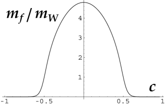
Figure 1: The lightest mass eigenvalue $m_{f}$ as a function of $c$ at $\theta_{W}=\hbox{${1\over 2}$}\pi$. The vertical axis is in the unit of $m_{W}$, or the fermion mass value at $c=\pm\frac{1}{2}$.

The remarkable fact is that the values of $c$ are distributed in the range $0.43<c<0.87$. The huge hierarchy in the quark-lepton masses is explained by standard distribution of $c$, which is a natural quantity in the RS spacetime. The mass becomes exponentially small for $c>0.6$.

	$m_{e}$	$m_{\mu}$	$m_{\tau}$	$m_{u}$	$m_{c}$	$m_{t}$
$c$	0.87	0.71	0.63	0.81	0.64	0.43

Table 1: The values of $c$ for leptons and quarks

6.1 Suppressed Yukawa couplings

By inserting the wave functions of the 4D Higgs field and fermions into $g_{A}\psi\kern-7.89993pt\raise 6.00006pt\hbox{$-$}\,\Gamma^{5}{e_{5}}^{y}A_{y}\psi$ and integrating over $y$, one finds the Yukawa coupling in four dimensions. In the standard model the Yukawa coupling is proportional to the mass of the fermion. The relation in the dynamical gauge-Higgs unification is modified, becoming

$$y_{\psi}\sim\frac{g_{A}\sqrt{k(c^{2}-\frac{1}{4})}}{2e^{\pi kR(c-\frac{1}{2})}}\cdot\cos\frac{\theta_{H}}{2}=\frac{gm_{f}}{2m_{W}}\cdot\cos^{2}\frac{\theta_{H}}{2}~{}~{}.$$ (26)

It is suppressed by a factor $\cos^{2}\hbox{${1\over 2}$}\theta_{H}$.

7 Gauge couplings of quarks and leptons

The electric charge is conserved and the electromagnetic coupling is universal. It is the same to all charged particles. The weak coupling constants, however, may not be universal once $SU(2)_{L}\times U(1)_{Y}$ breaks down to $U(1)_{\rm EM}$. In the standard model those weak couplings are universal at least at the tree level. In the dynamical gauge-Higgs unification small deviation results.

Each fermion multiplet couples to the $W$ boson with $g_{(0)}(\theta_{H},c)$ obtained by integrating over $y$ with wave functions of $W$ and fermions inserted in the gauge interaction term in (23). $g_{(0)}$ depends on both $\theta_{H}$ and $c$. It is depicted in fig. 2 as a function of $c=M/k$ at $\theta_{H}=\hbox{${1\over 2}$}\pi$. For $c>\hbox{${1\over 2}$}$ the deviation is very small. The asymptotic value for $c<\hbox{${1\over 2}$}$ is $\cos\theta_{H}$ in the $SU(3)$ model.

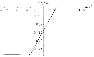
Figure 2: The 4D gauge coupling $g_{(0)}/g_{4}$ as a function of $c=M/k$ for $\theta_{W}=\hbox{${1\over 2}$}\pi$ and $kR=12$ in the $SU(3)$ model.

For the values of $c(>0.43)$ for quarks and leptons in table 1, the dependence of $g_{(0)}$ on $c$ is small. The violation of the $\mu$-$e$, $\tau$-$e$, and $t$-$e$ universality in the charged current interactions is of order of $10^{-8}$, $2\times 10^{-6}$ and $2\times 10^{-2}$, respectively.

Each quarks and leptons couples to the KK excited states of gauge bosons as well. It was noticed that those couplings can be large at $c=0$, which gives rise to contradition with observation unless $M_{KK}$ is sufficiently large.

The coupling $g_{(n)}$ of a fermion to the $n$-th KK excited state of $W$ is depicted in fig. 3 at $\theta_{H}=\hbox{${1\over 2}$}$. It is seen that the couplings are very small for $c>\hbox{${1\over 2}$}$ as noted by Gherghetta and Pomarol so that the earlier constgraint on $M_{KK}$ is evaded.

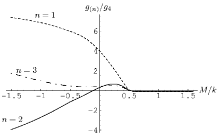
Figure 3: The gauge couplings to the $n$-th KK excited states of $W$, $g_{(n)}$ ($n=1,2,3$) as functions of $c=M/k$ at $\theta_{W}=\hbox{${1\over 2}$}\pi$ in the $SU(3)$ model.

8 $WWZ$, $WWH$, and $ZZH$ couplings

At $\theta_{H}\not=0$, an eigenstate of each field becomes mixture of various components of the multiplet which the field belong to. All of the $W$, $Z$, and $H$ fields in four dimensions are parts of the gauge field multiplets. The mixing pattern is not identical among these fields so that the effective 4D couplings necessarily depend on $\theta_{H}$. This would provide critical tests for the dynamical gauge-Higgs unification particularly in the $WWZ$, $WWH$, and $ZZH$ couplings.

The $WWZ$ coupling is found to be

$$g_{WWZ}\simeq g\cos\theta_{W}~{}.$$ (27)

To this order the coupling is the same as in the standard model. The experiment at LEP2 indicates the validity of the standard model.

The $WWH$ and $ZZH$ couplings are found to be

$$\hskip-28.45274pt\lambda_{WWH}\simeq gm_{W}\cdot p_{H}\cos\theta_{H}~{}~{},$$ (28)

$$\hskip-28.45274pt\lambda_{ZZH}\simeq\frac{gm_{Z}}{\cos\theta_{W}}\cdot p_{H}\cos\theta_{H}~{}~{},$$ (29)

where $p_{H}={\rm sign}(\sin\theta_{H})$. These couplings are suppressed by a factor $\cos\theta_{H}$. Note that these couplings are important in drawing a constraint for the Higgs boson mass from the LEP data as well.

Acknowledgments

The author would like to thank the Aspen Center for Physics for its hospitality where a part of this work was performed. This work was supported in part by Scientific Grants from the Ministry of Education and Science, Grant No. 17540257, Grant No. 13135215 and Grant No. 18204024.

References

References

- [1] Y. Hosotani, Phys. Lett. B126 (1983) 309.
- [2] Y. Hosotani, Ann. Phys. (N.Y.) 190 (1989) 233.
- [3] D.B. Fairlie, Phys. Lett. B82 (1979) 97; J. Phys. G5 (1979) L55.
- [4] N. Manton, Nucl. Phys. B158 (1979) 141.
- [5] H. Hatanaka, T. Inami and C.S. Lim, Mod. Phys. Lett. A13 (1998) 2601.
- [6] I. Antoniadis, K. Benakli and M. Quiros, New. J. Phys.3 (2001) 20.
- [7] M. Kubo, C.S. Lim and H. Yamashita, Mod. Phys. Lett. A17 (2002) 2249.
- [8] C. Csaki, C. Grojean and H. Murayama, Phys. Rev. D67 (2003) 085012; C.A. Scrucca, M. Serone and L. Silverstrini, Nucl. Phys. B669 (2003) 128.
- [9] L.J. Hall, Y. Nomura and D. Smith, Nucl. Phys. B639 (2002) 307; L. Hall, H. Murayama, and Y. Nomura, Nucl. Phys. B645 (2002) 85; G. Burdman and Y. Nomura, Nucl. Phys. B656 (2003) 3; C.A. Scrucca, M. Serone, L. Silvestrini and A. Wulzer, JHEP 0402 (2004) 49.
- [10] N. Haba, M. Harada, Y. Hosotani and Y. Kawamura, Nucl. Phys. B657 (2003) 169; Erratum, ibid. B669 (2003) 381.
- [11] N. Haba, Y. Hosotani, Y. Kawamura and T. Yamashita, Phys. Rev. D70 (2004) 015010; N. Haba, K. Takenaga, and T. Yamashita, Phys. Lett. B615 (2005) 247.
- [12] Y. Hosotani, S. Noda and K. Takenaga, Phys. Lett. B607 (2005) 276.
- [13] G. Cacciapaglia, C. Csaki and S.C. Park, JHEP 0603 (2006) 099.
- [14] G. Panico, M. Serone and A. Wulzer, Nucl. Phys. B739 (2006) 186.
- [15] R. Contino, Y. Nomura and A. Pomarol, Nucl. Phys. B671 (2003) 148.
- [16] K. Agashe, R. Contino and A. Pomarol, Nucl. Phys. B719 (2005) 165.
- [17] K. Oda and A. Weiler, Phys. Lett. B606 (2005) 408.
- [18] Y. Hosotani and M. Mabe, Phys. Lett. B615 (2005) 257.
- [19] Y. Hosotani, S. Noda, Y. Sakamura and S. Shimasaki, Phys. Rev. D73 (2006) 096006.
- [20] M. Carena, E. Ponton, J. Santiago and C.E.M. Wagner, hep-ph/0607106.
- [21] Y. Sakamura and Y. Hosotani, hep-ph/0607236.
- [22] Y. Hosotani, in the Proceedings of “Dynamical Symmetry Breaking”, ed. M. Harada and K. Yamawaki (Nagoya University, 2004), p. 17. (hep-ph/0504272).
- [23] N. Irges and F. Knechtli, Nucl. Phys. B719 (2005) 121; hep-lat/0604006.
- [24] N. Maru and T. Yamashita, hep-ph/0603237.
- [25] Y. Hosotani, hep-ph/0607064.
- [26] L. Randall and R. Sundrum, Phys. Rev. Lett. 83 (1999) 3370.
- [27] T. Gherghetta and A. Pomarol, Nucl. Phys. B586 (2000) 141.
- [28] S. Chang, J. Hisano, H. Nakano, N. Okada and M. Yamaguchi, Phys. Rev. D62 (2000) 084025.