Semi-analytical solution for Bogolubov’s angle $\theta(p)$ in the ’t Hooft model

Abstract

The analytical ansatz was found for Bogolubov’s angle $\theta(p)$ in the ’t Hooft model at $N\rightarrow\infty$. The appropriate calculations were done and final numeric approximation was found for this angle $\theta(p)$.

1. Introduction

There is a well known generalization of QCD from three colors to $N$ ($N\in\mathbb{N}$) colors or, in other words, from an $SU(3)$ gauge group to an $SU(N)$ gauge group which was done by t’Hooft [1]. t’ Hooft made this generalization because he hoped that model with a large $N$ (strictly speaking with limit $N\rightarrow\infty$, the so-called t’Hooft limit) might have an exact solution and might be qualitatively and quantitatively close to the actual QCD with $N=3$. His hope was justified; theory in the $N\rightarrow\infty$ limit has a considerable simplification. The fact is that we should take into account only planar diagrams, because others vanish [2]: “In the actual world quarks belong to the fundamental representation of $SU(3)$. If we assume that this assignment stays intact in multicolor QCD, each extra quark loop is suppressed by $1/N$. Therefore, in the ’t Hooft limit each process is saturated by contributions with the minimal possible number of quark loops”. This is the main reason we are motivated to investigate this model and to find a solution for Bogolubov’s angle.

All definitions and formulas which were necessary for presented calculations were taken from the paper [2].

2. Analytical ansatz for $\theta(p)$

The starter formulas for further calculations:

$$\begin{array}[]{l}E_{p}\cos\theta(p)-m=\dfrac{\gamma}{2}\int dk\cos\theta(k)\dfrac{1}{(p-k)^{2}}\,,\\ E_{p}\sin\theta(p)-p=\dfrac{\gamma}{2}\int dk\sin\theta(k)\dfrac{1}{(p-k)^{2}}\,,\end{array}$$ (1)

with the boundary conditions

$$\theta(p)\rightarrow\left\{\begin{array}[]{l}\phantom{-}\dfrac{\pi}{2}\quad\mbox{at}\quad p\rightarrow\infty\\[8.5359pt] -\dfrac{\pi}{2}\quad\mbox{at}\quad p\rightarrow-\infty\end{array}\right.$$ (2)

determined by the free-quark limit. This set of equations was firstly obtained by Bars and Green [3]. The angle $\theta(p)$ is referred to as the Bogolubov’s angle, or more commonly, the chiral angle.

From these equations one can easily get the following integral equation for the Bogolubov’s angle [3, 4]:

$$p\cos\theta(p)-m\sin\theta(p)=\dfrac{\gamma}{2}\int dk\sin\left(\theta(p)-\theta(k)\right)\dfrac{1}{(p-k)^{2}}\;.$$ (3)

Assuming that the chiral angle was found the following integral equation for the $E_{p}$ was obtained in paper [3, 4]:

$$E_{p}=m\cos\theta(p)+p\sin\theta(p)+\dfrac{\gamma}{2}\int dk\cos\left(\theta(p)-\theta(k)\right)\dfrac{1}{(p-k)^{2}}\;.$$ (4)

All calculations were performed in the limit of quark mass $m=0$. Thus, one can rewrite Eq. (3) and Eq. (4) in this limit.

$$p\cos{\theta(p)}=\frac{\displaystyle\gamma}{\displaystyle 2}\int\limits_{-\infty}^{\infty}\frac{\displaystyle{\sin[\theta(p)-\theta(k)]}}{\displaystyle{(p-k)^{2}}}\,\,dk\;,$$ (5)

$$E_{p}=p\sin\theta(p)+\dfrac{\gamma}{2}\int\dfrac{\cos\left(\theta(p)-\theta(k)\right)}{(p-k)^{2}}\,\,dk\;.$$ (6)

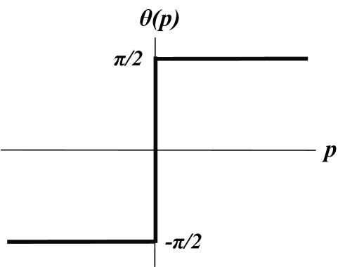
The exact singular analytical solution of the integral equation (5) is

$$\theta(p)=\frac{\displaystyle\pi}{\displaystyle 2}\,\mbox{sign}(p)\;,$$ (7)

where sign$(p)$ is the sign function

$$\mbox{sign}(p)=\vartheta(p)-\vartheta(-p)\;.$$

Figure 1: The analytical solution for Bogolubov’s angle $\theta(p)$ vs. $p$.

Substituting this solution in Eq. (6) we can get

$$E_{p}=|p|-\dfrac{\gamma}{|p|}\;.$$ (8)

However, this analytical solution is unphysical [2] for several reasons. For example, $E(p)$ becomes negative at $|p|<\sqrt{\gamma}$. This feature of the solution (8) cannot be amended by a change in the infrared regularization. In fact, solution (8) does not correspond to the minimum of the vacuum energy [5].

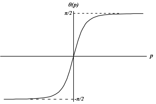
A stable solution has the form depicted in Fig. 2. It is smooth everywhere. At $|p|\ll\sqrt{\gamma}$ it is linear in $p$.

Figure 2: A stable solution for Bogolubov’s angle $\theta(p)$ vs. $p$.

For the convenience of the further calculations, the system of units in which $\gamma=1$ was used. The asymptotic behavior of the physical $\theta(p)$ [2]:

$$\begin{array}[]{lll}\theta(p)\sim p&\mbox{for }|p|\ll 1&\\[-7.11317pt] &&\mbox{and}\\[-7.11317pt] \theta(p)=\frac{\displaystyle\pi}{\displaystyle 2}\,\mbox{sign}(p)-\frac{\displaystyle\pi}{\displaystyle\sqrt{6}}\left(\frac{\displaystyle 1}{\displaystyle p}\right)^{3}+\cdots&\mbox{for }|p|\gg 1\;.&\end{array}$$ (9)

The asymptotic behavior of $\theta(p)$ at $|p|\gg 1$ was calculated by calculating the chiral quark condensate $\langle\bar{\psi}\psi\rangle$ for the smooth physical solution as a self-consistency condition [6].

Taking these asymptotics into account, we can find the analytical function for $\theta(p)$ which we can use to fit physical $\theta(p)$. Therefore the analytical ansatz for $\theta(p)$ is

$$\boxed{\;\theta(p)=\frac{\displaystyle 6ap}{\displaystyle 2+\pi\sqrt{6}a^{3}+6a^{2}p^{2}}+\arctan{(ap)}}\;,$$ (10)

where $a$ is a free parameter and $a>0$.
For any $a$, this ansatz gives the exact asymptotic behavior of the physical $\theta(p)$:

$$\begin{array}[]{rrr}\!\!\!\!\theta(p)=&&\\ &=\left(1+\dfrac{6}{2+\pi\sqrt{6}a^{3}}\right)ap+\dfrac{1}{3}\left(1+\dfrac{108}{\left(2+\pi\sqrt{6}a^{3}\right)^{2}}\right)a^{3}p^{3}+\cdots&\mbox{for }|p|\ll 1\\[-4.26773pt] &&\mbox{and}\\[-17.07182pt] \\ \theta(p)=&&\\ &=\frac{\displaystyle\pi}{\displaystyle 2}\,\mbox{sign}(p)-\frac{\displaystyle\pi}{\displaystyle\sqrt{6}}\frac{\displaystyle 1}{\displaystyle{p^{3}}}+\dfrac{5\pi a^{3}\left(3\pi a^{3}+2\sqrt{6}\right)-8}{90}\cdot\frac{\displaystyle 1}{\displaystyle{a^{5}p^{5}}}+\cdots&\mbox{for }|p|\gg 1\,.\end{array}$$ (11)

The graph of the physical $\theta(p)$ from this ansatz looks exactly like the curve on Fig. 2.

3. Numeric solution of $\theta(p)$

Mathematica 5.1 was employed to create a computer program for numerical calculations. Also for these calculations the analytical ansatz was used and it was found that, within precision of the calculations, the best fit of the analytical ansatz for $\theta(p)$ is reached when $a=0.3701$.

The precision of the calculations is $0.0001$. The discrepancy of a solution of the integral equation (5) at $\gamma=1$ is calculated by the formula:

$$\begin{array}[]{ll}S(a,p)=&\\ &=\dfrac{1}{\sqrt{n-1}}\sqrt{\sum\limits^{n}_{i=0}\left(p_{i}\cos{\theta_{\mbox{\scriptsize{calc}}}(p_{i},a)}-\frac{\displaystyle 1}{\displaystyle 2}\int\limits_{-\infty}^{\infty}\frac{\displaystyle{\sin[\theta_{\mbox{\scriptsize{calc}}}(p_{i},a)-\theta_{\mbox{\scriptsize{calc}}}(k,a)]}}{\displaystyle{(p_{i}-k)^{2}}}\,\,dk\right)^{2}}\\ \end{array}$$ (12)

where $n$ is a number of points in which $\theta_{\mbox{\scriptsize{calc}}}(p_{i})$ was calculated.

The dependence of $S(a,p)$ on momentum $p$ is an indirect dependence. This dependence is realized by the dependence of $S(a,p)$ on the choice of range of momentum $p$ and on the fragmentation of this range.

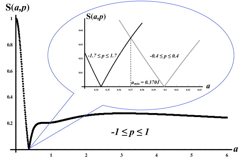
Figure 3: The dependence of the solution discrepancy of the integral equation for $\theta(p)$ on the parameter $a$.

The calculations of the solution discrepancy $S(a,p)$ shows that there are two local maximums of this discrepancy dependent on momentum $p$ near $p=0.4$ and $p=1.7$ momentum units. Investigating the dependence of the discrepancy on parameter $a$ at this region of momentum $p$, it was found that the discrepancy $S(a,p)$ of the calculations is bounded above $0.035$, and that it reaches the minimum at $a=0.3701$.

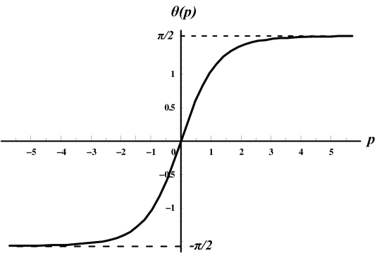
For the case $a=0.3701$, the solution for the physical Bogolubov’s angle $\theta(p)$ was obtained:

$$\boxed{\;\theta(p)=\dfrac{2.2206}{2.3901+0.8218\,p^{2}}\,p+\arctan\left(0.3701p\right)}\;.$$ (13)

Figure 4: The best fit at $a=0.3701$ for the physical solution of the Bogolubov’s angle $\theta(p)$ vs. $p$.

The asymptotic behavior of physical $\theta(p)$:

$$\begin{array}[]{lll}\theta(p)=1.2992p-0.3364p^{3}+\cdots&\mbox{for }|p|\ll 1&\\[-4.26773pt] &&\mbox{and}\\[-17.07182pt] \\ \theta(p)=\frac{\displaystyle\pi}{\displaystyle 2}\,\mbox{sign}(p)-\frac{\displaystyle\pi}{\displaystyle\sqrt{6}}\frac{\displaystyle 1}{\displaystyle{p^{3}}}-5.9502\frac{\displaystyle 1}{\displaystyle{p^{5}}}+\cdots&\mbox{for }|p|\gg 1\,.&\end{array}$$ (14)

4. Conclusions

The essential advantage of the suggested technique for calculations of the $\theta(p)$ is that they are based on the exact asymptotic behavior of the physical Bogolubov’s angle $\theta(p)$ at $p\rightarrow 0$ and at $p\rightarrow\pm\infty$. This gives us an opportunity to call the obtained solution for $\theta(p)$ a semi-analytical one.

The accuracy of my calculations is $0.035$ or better. This error appears when momentum $p$ is about either $0.4$ or $1.7$ momentum units. However, when the absolute value of momentum is less than $0.02$ or greater than $4.9$ momentum units, the accuracy has already been an order of magnitude better, i.e. an accuracy about $0.003$.

If less of the solution discrepancy of the integral equation for $\theta(p)$ is needed, we suppose the accuracy of calculations can be improved by adding terms of high order of $p$ to the trial function of $\theta(p)$.

References

[1]
G. ’t Hooft, Nucl. Phys.B 72,(1974) 461;
G. t’Hooft, Nucl. Phys.B 75, (1974) 461 . [Reprinted
in G. t’Hooft, Under the Spell of the Gauge Principle,
(World Scientific, Singapure, 1994), p. 461].
[2]
M. Shifman, A Lecutre on ’t Hooft Model to be published.
[3]
I. Bars and M.B. Green, Phys. Rev.D 17 (1978) 537.
[4]
F. Lenz, M. Thies, S. Levit, and K. Yazaki, Ann. Phys. (N.