Grand Unified Theories

Stuart Raby

Department of Physics, The Ohio State University, 191 W. Woodruff Ave.

Columbus, OH 43210

Invited talk given at the 2nd World Summit on Physics Beyond the Standard Model

Galapagos Islands, Ecuador June 22-25, 2006

1 Grand Unification

The standard model is specified by the local gauge symmetry group, $SU(3)\times SU(2)\times U(1)_{Y}$, and the charges of the matter particles under the symmetry. One family of quarks and leptons [${Q,u^{c},d^{c};L,e^{c}}$] transform as [$(3,2,1/3),$ $({\bar{3}},1,-4/3),$ $({\bar{3}},1,2/3);$ $(1,2,-1),$ $(1,1,2)$], where $Q=(u,d)$ and $L=(\nu,e)$ are $SU(2)_{L}$ doublets and $u^{c},\;d^{c},\;e^{c}$ are charge conjugate $SU(2)_{L}$ singlet fields with the $U(1)_{Y}$ quantum numbers given. [We use the convention that electric charge $Q_{EM}=T_{3L}+Y/2$ and all fields are left handed.] Quark, lepton, W and Z masses are determined by dimensionless couplings to the Higgs boson and the neutral Higgs vev. The apparent hierarchy of fermion masses and mixing angles is a complete mystery in the standard model. In addition, light neutrino masses are presumably due to a See-Saw mechanism with respect to a new large scale of nature.

The first unification assumption was made by Pati and Salam [PS] [1] who proposed that lepton number was the fourth color, thereby enlarging the color group $SU(3)$ to $SU(4)$. They showed that one family of quarks and leptons could reside in two irreducible representations of a left-right symmetric group $SU(4)\times SU(2)_{L}\times SU(2)_{R}$ with weak hypercharge given by $Y/2=1/2(B-L)+T_{3R}$. Thus in PS, electric charge is quantized.

Shortly after PS was discovered, it was realized that the group $SO(10)$ contained PS as a subgroup and unified one family of quarks and leptons into one irreducible representation, 16 [2]. See Table 1. This is clearly a beautiful symmetry, but is it realized in nature? If yes, what evidence do we have?

Table 1: The quantum numbers of the ${\bf 16}$ dimensional representation of $SO(10)$.

$$\begin{array}[]{|c|c|c|c|}\hline\cr{\rm State}&Y&{\rm Color}&{\rm Weak}\\ \hline\cr\hline\cr{\bf\nu^{c}}&0&+\,+\,+&+\,+\\ \hline\cr\hline\cr{\bf e^{c}}&2&+\,+\,+&-\,-\\ \hline\cr{\bf u_{r}}&1/3&-\,+\,+&+\,-\\ {\bf d_{r}}&1/3&-\,+\,+&-\,+\\ \hline\cr{\bf u_{b}}&1/3&+\,-\,+&+\,-\\ {\bf d_{b}}&1/3&+\,-\,+&-\,+\\ \hline\cr{\bf u_{y}}&1/3&+\,+\,-&+\,-\\ {\bf d_{y}}&1/3&+\,+\,-&-\,+\\ \hline\cr{\bf u_{r}^{c}}&-4/3&+\,-\,-&+\,+\\ {\bf u_{b}^{c}}&-4/3&-\,+\,-&+\,+\\ {\bf u_{y}^{c}}&-4/3&-\,-\,+&+\,+\\ \hline\cr\hline\cr{\bf d_{r}^{c}}&2/3&+\,-\,-&-\,-\\ {\bf d_{b}^{c}}&2/3&-\,+\,-&-\,-\\ {\bf d_{y}^{c}}&2/3&-\,-\,+&-\,-\\ \hline\cr{\bf\nu}&-1&-\,-\,-&+\,-\\ {\bf e}&-1&-\,-\,-&-\,+\\ \hline\cr\end{array}$$

Of course, grand unification makes several predictions. The first two being gauge coupling unification and proton decay [3, 4]. Shortly afterward it was realized that Yukawa unification was also predicted [5]. Experiments looking for proton decay were begun in the early 80s. By the late 80s it was realized that grand unification apparently was not realized in nature (assuming the standard model particle spectrum). Proton decay was not observed and in 1992, LEP data measuring the three standard model fine structure constants $\alpha_{i},\ i=1,2,3$ showed that non-supersymmetric grand unification was excluded by the data [6]. On the other hand, supersymmetric GUTs [7] (requiring superpartners for all standard model particles with mass of order the weak scale) was consistent with the LEP data [6] and at the same time raised the GUT scale; thus suppressing proton decay from gauge boson exchange [7]. See Fig. 1.

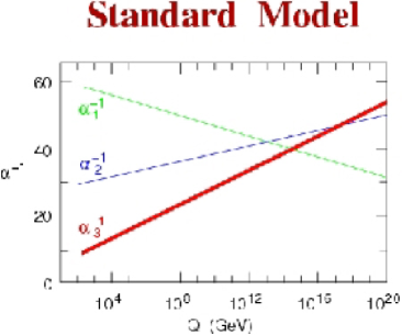
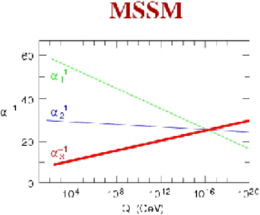
Figure 1: Gauge coupling unification in non-SUSY GUTs (top) vs. SUSY GUTs (bottom) using the LEP data as of 1991. Note, the difference in the running for SUSY is the inclusion of supersymmetric partners of standard model particles at scales of order a TeV.

The spectrum of the minimal SUSY theory includes all the SM states plus their supersymmetric partners. It also includes one pair (or more) of Higgs doublets; one to give mass to up-type quarks and the other to down-type quarks and charged leptons. Two doublets with opposite hypercharge $Y$ are also needed to cancel triangle anomalies. Finally, it is important to recognize that a low energy SUSY breaking scale (the scale at which the SUSY partners of SM particles obtain mass) is necessary to solve the gauge hierarchy problem.

SUSY extensions of the SM have the property that their effects decouple as the effective SUSY breaking scale is increased. Any theory beyond the SM must have this property simply because the SM works so well. However, the SUSY breaking scale cannot be increased with impunity, since this would reintroduce a gauge hierarchy problem. Unfortunately there is no clear-cut answer to the question, when is the SUSY breaking scale too high. A conservative bound would suggest that the third generation quarks and leptons must be lighter than about 1 TeV, in order that the one loop corrections to the Higgs mass from Yukawa interactions remains of order the Higgs mass bound itself.

SUSY GUTs can naturally address all of the following issues:

• $M_{Z}\ll M_{GUT}$ Natural

• Explains charge quantization

• Predicts gauge coupling unification !!

• Predicts SUSY particles at LHC

• Predicts proton decay

• Predicts Yukawa coupling unification

• and with broken Family symmetry explains the fermion mass hierarchy

• Neutrino masses and mixing via See-Saw

• LSP - Dark Matter candidate

• Baryogenesis via leptogenesis

In this talk, I will consider two topics. The first topic is a comparison of GUT predictions in the original 4 dimensional field theory version versus its manifestation in 5 or 6 dimensional orbifold field theories (so-called orbifold GUTs) or in the 10 dimensional heterotic string. The second topic focuses on the minimal SO(10) SUSY model [MSO₁₀SM]. By definition, in this theory the electroweak Higgs of the MSSM is contained in a single 10 dimensional representation of SO(10). There are many experimentally verifiable consequences of this theory. This is due to the fact that

1. in order to fit the top, bottom and tau masses one finds that the SUSY breaking soft terms are severely constrained, and

2. the ratio of the two Higgs vevs, $\tan\beta\sim 50$. This by itelf leads to several interesting consequences.

2 Gauge coupling unification & Proton decay

2.1 4D GUTs

At $M_{G}$ the GUT field theory matches on to the minimal SUSY low energy theory with matching conditions given by $g_{3}=g_{2}=g_{1}\equiv g_{G}$, where at any scale $\mu<M_{G}$ we have $g_{2}\equiv g$ and $g_{1}=\sqrt{5/3}\;g^{\prime}$. Then using two low energy couplings, such as $\alpha_{EM}(M_{Z}),\;\sin^{2}\theta_{W}$, the two independent parameters $\alpha_{G},\;M_{G}$ can be fixed. The third gauge coupling, $\alpha_{s}(M_{Z})$ is predicted.

At present gauge coupling unification within SUSY GUTs works extremely well. Exact unification at $M_{G}$, with two loop renormalization group running from $M_{G}$ to $M_{Z}$, and one loop threshold corrections at the weak scale, fits to within 3 $\sigma$ of the present precise low energy data. A small threshold correction at $M_{G}$ ($\epsilon_{3}\sim$ - 3% to - 4%) is sufficient to fit the low energy data precisely [8, 9, 10]. See Fig. 2. This may be compared to non-SUSY GUTs where the fit misses by $\sim$ 12 $\sigma$ and a precise fit requires new weak scale states in incomplete GUT multiplets or multiple GUT breaking scales. When GUT threshold corrections are considered, then all three gauge couplings no longer meet at a point. Thus we have some freedom in how we define the GUT scale. We choose to define the GUT scale as the point where $\alpha_{1}(M_{G})=\alpha_{2}(M_{G})\equiv\tilde{\alpha}_{G}$ and $\alpha_{3}(M_{G})=\tilde{\alpha}_{G}\;(1+\epsilon_{3})$. The threshold correction $\epsilon_{3}$ is a logarithmic function of all states with mass of order $M_{G}$ and $\tilde{\alpha}_{G}=\alpha_{G}+\Delta$ where $\alpha_{G}$ is the GUT coupling constant above $M_{G}$ and $\Delta$ is a one loop threshold correction. To the extent that gauge coupling unification is perturbative, the GUT threshold corrections are small and calculable. This presumes that the GUT scale is sufficiently below the Planck scale or any other strong coupling extension of the GUT, such as a strongly coupled string theory.

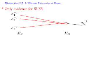
Figure 2: Gauge coupling unification in SUSY GUTs using the LEP data. Given the present accurate measurements of the three low energy couplings, in particular $\alpha_{s}(M_{Z})$, and the fact that the theoretical analysis now requires two loop RG running from $M_{G}$ to $M_{Z}$ and one loop threshold corrections at the weak scale; GUT scale threshold corrections are now needed to precisely fit the low energy data.

In four dimensional SUSY GUTs, the threshold correction $\epsilon_{3}$ receives a positive contribution from Higgs doublets and triplets. Note, the Higgs contribution is given by $\epsilon_{3}={3\tilde{\alpha}_{G}\over 5\pi}\log|{\tilde{M_{t}}\ \gamma\over M_{G}}|$ where $\tilde{M_{t}}$ is the effective color triplet Higgs mass (setting the scale for dimension 5 baryon and lepton number violating operators) and $\gamma=\lambda_{b}/\lambda_{t}$ at $M_{G}$. Obtaining $\epsilon_{3}\sim-3\%$ (with $\gamma=1$) requires $\tilde{M_{t}}\sim 10^{14}$ GeV. Unfortunately this value of $\tilde{M_{t}}$ is now excluded by the non-observation of proton decay. In fact, as we shall now discuss, the dimension 5 operator contribution to proton decay requires $\tilde{M_{t}}$ to be greater than $M_{G}$. In this case the Higgs contribution to $\epsilon_{3}$ is positive. Thus a larger, negative contribution must come from the GUT breaking sector of the theory. This is certainly possible in specific SO(10)  [12] or SU(5)  [13] models, but it is clearly a significant constraint on the 4d GUT-breaking sector of the theory.

Baryon number is necessarily violated in any GUT [14]. In any grand unified theory, nucleons decay via the exchange of gauge bosons with GUT scale masses, resulting in dimension 6 baryon number violating operators suppressed by $(1/M_{G}^{2})$. The nucleon lifetime is calculable and given by $\tau_{N}\propto M_{G}^{4}/(\alpha_{G}^{2}\;m_{p}^{5})$. The dominant decay mode of the proton (and the baryon violating decay mode of the neutron), via gauge exchange, is $p\rightarrow e^{+}\;\pi^{0}$ ($n\rightarrow e^{+}\;\pi^{-}$). In any simple gauge symmetry, with one universal GUT coupling and scale ($\alpha_{G},\;M_{G}$), the nucleon lifetime from gauge exchange is calculable. Hence, the GUT scale may be directly observed via the extremely rare decay of the nucleon. The present experimental bounds come from Super-Kamiokande. We discuss these results shortly. In SUSY GUTs, the GUT scale is of order $3\times 10^{16}$ GeV, as compared to the GUT scale in non-SUSY GUTs which is of order $10^{15}$ GeV. Hence the dimension 6 baryon violating operators are significantly suppressed in SUSY GUTs [7] with $\tau_{p}\sim 10^{34-38}$ yrs.

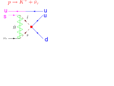
Figure 3: The contribution of dimension 5 operators to proton decay. The red dot denotes the dimension 5 vertex.

However, in SUSY GUTs there are additional sources for baryon number violation – dimension 4 and 5 operators [15]. The dimension 4 operators violate baryon number or lepton number, respectively, but not both. The nucleon lifetime is extremely short if both types of dimension 4 operators are present in the low energy theory. However both types can be eliminated by requiring R parity [16]. R parity distinguishes Higgs multiplets from ordinary families. In $SU(5)$, Higgs and quark/lepton multiplets have identical quantum numbers; while in $E(6)$, Higgs and families are unified within the fundamental ${\bf 27}$ representation. Only in SO(10) are Higgs and ordinary families distinguished by their gauge quantum numbers. In what follows we shall assume that R parity is a good symmetry and neglect further discussion of Dimension 4 baryon and/or lepton number violating operators. As a consequence, the lightest SUSY particle [LSP] is stable and is an excellent dark matter candidate.

The dimension 5 operators have a dimensionful coupling of order ($1/M_{G}$). Dimension 5 baryon number violating operators may be forbidden at tree level by symmetries in $SU(5)$, etc. These symmetries are typically broken however by the VEVs responsible for the color triplet Higgs masses. Consequently these dimension 5 operators are generically generated via color triplet Higgsino exchange. Hence, the color triplet partners of Higgs doublets must necessarily obtain mass of order the GUT scale. The dominant decay modes from dimension 5 operators are $p\rightarrow K^{+}\;\bar{\nu}\;\;(n\rightarrow K^{0}\;\bar{\nu})$. See Fig. 3. This is due to a simple symmetry argument; the operators $(Q_{i}\;Q_{j}\;Q_{k}\;L_{l}),\;\;(u^{c}_{i}\;u^{c}_{j}\;d^{c}_{k}\;e^{c}_{l})$ (where $i,\;j,\;k,\;l=1,2,3$ are family indices and color and weak indices are implicit) must be invariant under $SU(3)_{C}$ and $SU(2)_{L}$. As a result their color and weak doublet indices must be anti-symmetrized. However since these operators are given by bosonic superfields, they must be totally symmetric under interchange of all indices. Thus the first operator vanishes for $i=j=k$ and the second vanishes for $i=j$. Hence a second or third generation member must exist in the final state [17].

Super-Kamiokande bounds on the proton lifetime severely constrain these dimension 6 and 5 operators with $\tau_{(p\rightarrow e^{+}\pi^{0})}>5.0\times 10^{33}$ yrs (79.3 ktyr exposure), $\tau_{(n\rightarrow e^{+}\pi^{-})}>5\times 10^{33}$ yrs (61 ktyr), and $\tau_{(p\rightarrow K^{+}\bar{\nu})}>2.3\times 10^{33}$ yrs (92 ktyr), $\tau_{(n\rightarrow K^{0}\bar{\nu})}>1.3\times 10^{32}$ yrs (92 ktyr) at (90% CL) based on the listed exposures [18]. These constraints are now sufficient to rule out minimal SUSY $SU(5)$ [19]. Non-minimal Higgs sectors in $SU(5)$ or $SO(10)$ theories still survive [9, 13]. The upper bound on the proton lifetime from these theories are approximately a factor of 5 above the experimental bounds. They are, however, being pushed to their theoretical limits. Hence if SUSY GUTs are correct, nucleon decay must be seen soon.

2.2 4D vs. Orbifold GUTs

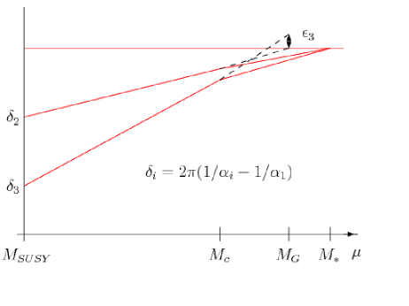
Figure 4: One loop RG running in orbifold GUTs from Kim and Raby [24].

Orbifold compactification of the heterotic string [20, 21, 22, 23], and recent field theoretic constructions known as orbifold GUTs [24], contain grand unified symmetries realized in 5 and 6 dimensions. However, upon compactifying all but four of these extra dimensions, only the MSSM is recovered as a symmetry of the effective four dimensional field theory. These theories can retain many of the nice features of four dimensional SUSY GUTs, such as charge quantization, gauge coupling unification and sometimes even Yukawa unification; while at the same time resolving some of the difficulties of 4d GUTs, in particular problems with unwieldy Higgs sectors necessary for spontaneously breaking the GUT symmetry, and problems with doublet-triplet Higgs splitting or rapid proton decay.

In five or six dimensional orbifold GUTs, on the other hand, the “GUT scale” threshold correction comes from the Kaluza-Klein modes between the compactification scale, $M_{c}$, and the effective cutoff scale $M_{*}$. Thus, in orbifold GUTs, gauge coupling unification at two loops is only consistent with the low energy data with a fixed value for $M_{c}$ and $M_{*}$. Typically, one finds $M_{c}<M_{G}(=3\times 10^{16}$ GeV) $<M_{*}$, where $M_{G}$ is the 4d GUT scale. Since the grand unified gauge bosons, responsible for nucleon decay, get mass at the compactification scale, the result $M_{c}<M_{G}$ for orbifold GUTs has significant consequences for nucleon decay. See Fig. 4.

Orbifold GUTs and string theories contain grand unified symmetries realized in higher dimensions. In the process of compactification and GUT symmetry breaking, color triplet Higgs states are removed (projected out of the massless sector of the theory). In addition, the same projections typically rearrange the quark and lepton states so that the massless states which survive emanate from different GUT multiplets. In these models, proton decay due to dimension 5 operators can be severely suppressed or eliminated completely. However, proton decay due to dimension 6 operators may be enhanced, since the gauge bosons mediating proton decay obtain mass at the compactification scale, $M_{c}$, which is less than the 4d GUT scale, or suppressed, if the states of one family come from different irreducible representations. Which effect dominates is a model dependent issue. In some complete 5d orbifold GUT models [27, 10] the lifetime for the decay $\tau(p\rightarrow e^{+}\pi^{0})$ can be near the excluded bound of $5\times 10^{33}$ years with, however, large model dependent and/or theoretical uncertainties. In other cases, the modes $p\rightarrow K^{+}\bar{\nu}$ and $p\rightarrow K^{0}\mu^{+}$ may be dominant [10]. To summarize, in either 4d or orbifold string/field theories, nucleon decay remains a premier signature for SUSY GUTs. Moreover, the observation of nucleon decay may distinguish extra-dimensional orbifold GUTs from four dimensional ones.

2.3 Heterotic string/orbifold GUTs

In recent years there has been a great deal of progress in constructing three and four family models in Type IIA string theory with intersecting D6 branes [28]. Although these models can incorporate SU(5) or a Pati-Salam symmetry group in four dimensions, they typically have problems with gauge coupling unification. In the former case this is due to charged exotics which affect the RG running, while in the latter case the SU(4)$\times$SU(2)${}_{L}\times$SU(2)_R symmetry never unifies. Note, heterotic string theory models also exist whose low energy effective 4d field theory is a SUSY GUT [29]. These models have all the virtues and problems of 4d GUTs. Finally, many heterotic string models have been constructed with the standard model gauge symmetry in 4d and no intermediate GUT symmetry in less than 10d. Recently some minimal 3 family supersymmetric models have been constructed [30, 31]. These theories may retain some of the symmetry relations of GUTs, however the unification scale would typically be the string scale, of order $5\times 10^{17}$ GeV, which is inconsistent with low energy data. A way out of this problem was discovered in the context of the strongly coupled heterotic string, defined in an effective 11 dimensions [32]. In this case the 4d Planck scale (which controls the value of the string scale) now unifies with the GUT scale.

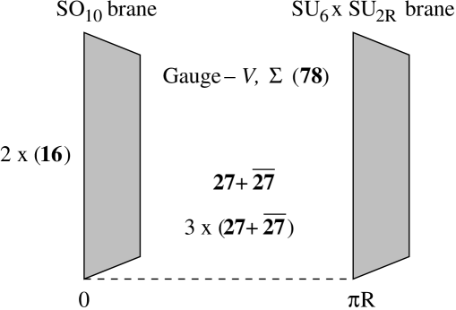
Figure 5: Schematic of an E(6) orbifold GUT in 5 dimensions with details in the text.

Recently a new paradigm has been proposed for using orbifold GUT intuition for constructing heterotic string models [22]. Consider an $E(6)$ orbifold GUT defined in 5 dimensions, where the 5th dimension is a line segment from $y=0$ to $\pi R$, as given in Fig. 5. In this theory the bulk contains the gauge hypermultiplet $V,\ \Sigma$ (in 4 dimensional N=1 SUSY notation) and four 27 dimensional hypermultiplets. The orbifold parities $Z_{2}\times Z_{2}^{\prime}$ leave an $SO(10)$ invariant brane at $y=0$ and an $SU(6)\times SU(2)_{R}$ invariant brane at $y=\pi R$. The overlap between these two localized symmetries is the low energy symmetry of the theory, which in this case is Pati-Salam. Note the theory also contains massless Higgs bosons necessary to spontaneously break PS to the standard model. In orbifold GUT language the compactification scale is given by $M_{c}=1/\pi R$ and the theory is cut-off at a scale $M_{*}\gg M_{c}$. In this theory we have the two light families of quarks and leptons residing on the $SO(10)$ brane, while the Higgs doublets and third family are located in the bulk. Finally the compactification scale is of order $7\times 10^{15}$ GeV. Thus proton decay via dimension 6 operators is enhanced, while proton decay via dimension 5 operators is forbidden.

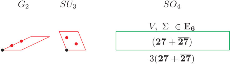
Figure 6: The bulk states in an effective 5D orbifold GUT obtained from the heterotic string. More details in the text.

Now let’s discuss how one obtains this model from the $E(8)\times E(8)$ heterotic string in 10 dimensions [22]. One compactifies 6 dimensions on 3 two dimensional torii defined by the root lattice of $G_{2}\times SU(3)\times SO(4)$ given in Fig. 6. One must also mod out by a $Z_{2}\times Z_{3}$ orbifold symmetry of the lattice. Consider first $(T^{2})^{3}/Z_{3}$ where the $Z_{3}$ twist is also embedded in the $E(8)\times E(8)$ group lattice via a shift vector $V_{3}$ and a Wilson line $W_{3}$ in the $SU(3)$ torus. Note, the $Z_{3}$ twist only acts on the $G_{2}\times SU(3)$ torii, leaving the $SO(4)$ torus untouched. As a result of the orbifolding, the $E(8)\times E(8)$ symmetry is broken to $E(6)\times$ an $SO(10)\times U(1)^{5}$ hidden sector gauge symmetry. We will not consider the hidden sector further in the discussion. The untwisted sector of the string contains the following massless states, $V,\ \Sigma$ in the adjoint of $E_{6}$ and one 27 dimensional hypermultiplet. Three more 27 dimensional hypermultiplets sit at the trivial fixed point in the $SU(3)$ torus and one each at the 3 $G_{2}$ fixed points. However at this level the massless string fields can be described by an effective 6 dimensional theory. Out of the 6 compactified dimensions we take 5 to be of order the string scale and one much larger than the string scale, as in Fig. 6. In this case, we now have the first step in the 5 dimensional orbifold GUT described earlier. In order to break the $E(6)$ gauge symmetry we now apply the $Z_{2}$ twist, acting on the $G_{2}\times SO(4)$ torii, and embedded into the $E(8)\times E(8)$ gauge lattice by a shift vector $V_{2}$ and a Wilson line, $W_{2}$, along the long axis of the $SO(4)$ torus. As a result we find the massless sector shown in Fig. 7.

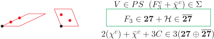
Figure 7: The bulk states in effective 5D orbifold GUT after the $Z_{2}$ twist and Wilson line. More details in the text.

The shift $V_{2}$ can be identified with the first orbifold parity leaving two $SO(10)$ invariant fixed points in the $SO(4)$ torus. While the combination $V_{2}+W_{2}$ leaves two $SU(6)\times SU(2)_{R}$ invariant fixed point at the opposite side of the orbifold. See Fig. 8 which describes the $T_{1}$ twisted sector of the string. Note we also find two complete 16 dimensional representations of $SO(10)$ residing, one on each of the $SO(10)$ fixed points.

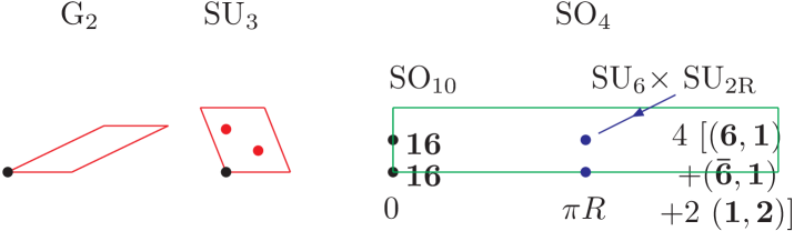
Figure 8: The twisted sector states in the $T_{1}$ twisted sector.

As a consequence of the string selection rules we find a $D_{4}$ family symmetry, where $D_{4}=\{\pm 1,\pm\sigma_{1},\pm\sigma_{3},\pm i\sigma_{2}\}$. The two light families transform as the fundamental doublet, where the action of $\sigma_{1}\ [\sigma_{3}]$ is given by $(f_{1},\ f_{1}^{c})\leftrightarrow(f_{2},\ f_{2}^{c})\;[(f_{2},\ f_{2}^{c})\leftrightarrow-(f_{2},\ f_{2}^{c})]$. The third family, given by the PS multiplets $f_{3}=(4,2,1)$ and $f_{3}^{c}=(\bar{4},1,\bar{2})$, and the Higgs doublet, ${\cal H}=(1,\bar{2},2)$, transform as $D_{4}$ singlets. As a result of the $D_{4}$ family symmetry, we find that the effective Yukawas for the theory are constrained to be of the form given in Fig. 9, where the terms $\tilde{S}_{e,o}$ are products of vevs of standard model singlets, even or odd under $\pm\sigma_{3}$ and $O_{1,2}$ are the vevs of PS breaking Higgs multiplets.

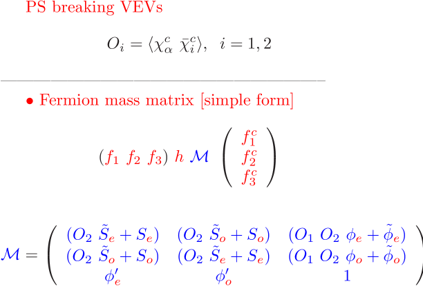
Figure 9:

Note the non-abelian family symmetry $D_{4}$ is a discrete subgroup of $SU(2)$. Unbroken $D_{4}$ symmetry requires degenerate masses for squarks and sleptons of the light two families, hence suppressing flavor violating processes such as $\mu\rightarrow e\gamma$ (Fig. 10).

Figure 10: One loop contribution to the process $\mu\rightarrow e\ \gamma$ in a SUSY flavor basis defined by lepton mass eigenstates, BUT not necessarily slepton mass eigenstates.

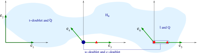
Figure 11: Some of the states obtained in a $(T^{2})^{3}/(Z_{2}\times Z_{4})$ orbifold compactification of the E(8) $\times$ E(8) heterotic string to the Standard Model gauge symmetry. See test for more details.

We are now performing a search in the “string landscape” for standard model theories in four dimensions compactified on a $(T^{2})^{3}/(Z_{2}\times Z_{3})$ or $(T^{2})^{3}/(Z_{2}\times Z_{4})$ orbifold [33]. These can be obtained with a combination of shift vectors V and up to 3 Wilson lines. Yes, we are searching for the MSSM in 4D without including GUTs.

Consider, for example, the case $(T^{2})^{3}/(Z_{2}\times Z_{4})$. The search strategy is to look for models with gauge group $SU(3)\times SU(2)\times U(1)^{n}\times$ a possible non-abelian hidden sector group. At the first step, we identify a three family model as one which has 3 more $({\bf 3,2})$ than $({\bf\bar{3},2})$, 6 more $({\bf\bar{3},1})$ than their conjugates and at least 5 $({\bf 1,2})$. The last condition guarantees that we have 3 families of lepton doublets and at least two higgs doublets. There are 120 inequivalent possibilities for the shift vectors $V_{2},\ V_{4}$. Then with either one or two Wilson lines we find 500,000 possible models.

However at this level, we have yet to identify the weak hypercharge as one linear combination of all the $U(1)$ charges. We find that, in general, the models satisfying this initial cut have non-standard model hypercharge assignments and in most cases, chiral exotics, i.e. fractionally charged states which cannot obtain mass. We then needed a search strategy to find standard model hypercharge assignments for quarks and leptons. Aha, if we require that the 3 families come in complete $SU(5)$ or PS multiplets, at an intermediate state AND identified hypercharge as $Y\in SU(5)$ or $Y=(B-L)+2T_{3R}\in PS$, then we found 3 family models with only vector-like exotics. Thus the hypothesis we are now testing is whether quarks and leptons coming from complete GUT multiplets are necessary for charge quantization. Our preliminary results are as follows, we find

1. 6 models via PS $\rightarrow$ SM, and

2. 40 models via $SU(5)\rightarrow$ SM .

If we now look for models with 3 families of quarks and leptons with Pati Salam symmetry in 4 dimensions and the necessary Higgs bosons to break PS to the standard model AND no chiral exotics, we find about 220 models.

One example of a three family model with vector-like exotics in $Z_{2}\times Z_{4}$ orbifold is given in Fig. 11. The top quark doublet, left-handed anti-top and $H_{u}$ reside in the bulk and has a tree level Yukawa coupling. The left-handed anti-bottom and tau lepton resides on twisted sector fixed points and their Yukawa couplings come only at order $S^{2}$. Finally the light two families come on two distinct fixed points in the twisted sector, although the description is a bit more complicated than our earlier model. We have not analyzed these models in any great detail, so for example, we do not know the complete family symmetry of the theory or whether all the vector-like exotics can get a large mass.

3 Minimal SO₁₀ SUSY Model [MSO₁₀SM] and Large $\tan\beta$

Let me first define what I mean by the [MSO₁₀SM] [34, 35, 36]. Quarks and leptons of one family reside in the $\bf 16$ dimensional representation, while the two Higgs doublets of the MSSM reside in a single $\bf 10$ dimensional representation. For the third generation we assume the minimal Yukawa coupling term given by ${\bf\lambda\ 16\ 10\ 16}.$ On the other hand, for the first two generations and for their mixing with the third, we assume a hierarchical mass matrix structure due to effective higher dimensional operators. Hence the third generation Yukawa couplings satisfy $\lambda_{t}=\lambda_{b}=\lambda_{\tau}=\lambda_{\nu_{\tau}}={\bf\lambda}$.

Soft SUSY breaking parameters are also consistent with $SO_{10}$ with (1) a universal gaugino mass $M_{1/2}$, (2) a universal squark and slepton mass $m_{16}$, (3) a universal scalar Higgs mass $m_{10}$, and (4) a universal A parameter $A_{0}$. In addition we have the supersymmetric (soft SUSY breaking) Higgs mass parameters $\mu$ ($B\mu$). $B\mu$ may, as in the CMSSM, be exchanged for $\tan\beta$. Note, not all of these parameters are independent. Indeed, in order to fit the low energy electroweak data, including the third generation fermion masses, it has been shown that $A_{0},\ m_{10},\ m_{16}$ must satisfy the constraints [34]

$$A_{0}\approx-2\ m_{16}; m_{10}\approx\sqrt{2}\ m_{16}$$ (1)

$$m_{16}>1.2\;{\rm TeV}; \mu,\ M_{1/2}\ll m_{16}$$ (2)

with

$$\tan\beta\approx 50.$$ (3)

3.1 Dark matter and WMAP data

The model is assumed to have a conserved R parity, thus the LSP is stable and an excellent dark matter candidate. In our case the LSP is a neutralino; roughly half higgsino and half gaugino. The dominant annihilation channel is via an s-channel CP odd Higgs, A. In the large $\tan\beta$ limit, A is a wide resonance since its coupling to bottom quarks and taus is proportional to $\tan\beta$. In Fig. 12 we give the fit to WMAP dark matter abundance as a function of $\mu,\ M_{1/2}$ for $m_{16}=3$ TeV and $m_{A}=700$ GeV [35]. The green (darker shaded) area is consistent with WMAP data. While to the left the dark matter abundance is too large and to the right (closer to the A peak) it is too small. In Fig. 13 we give the spin independent neutralino-proton cross-section relevant for dark matter searches. All the points give acceptable fits for top, bottom and tau masses, as well as $\alpha_{i},\ i=1,2,3$ at $M_{Z}$ with $Br(B_{s}\rightarrow\mu^{+}\mu^{-})\leq 5\times 10^{-7}$. The large dots also satisfy $Br(B_{s}\rightarrow\mu^{+}\mu^{-})\leq 2\times 10^{-7}$.

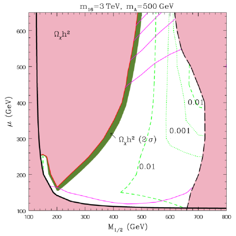
Figure 12: Neutralino dark matter abundance from Ref. [35].

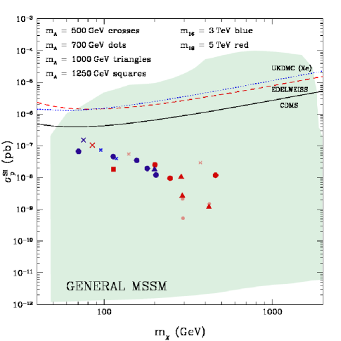
Figure 13: Spin-independent neutralino - proton scattering cross-section from Ref. [35].

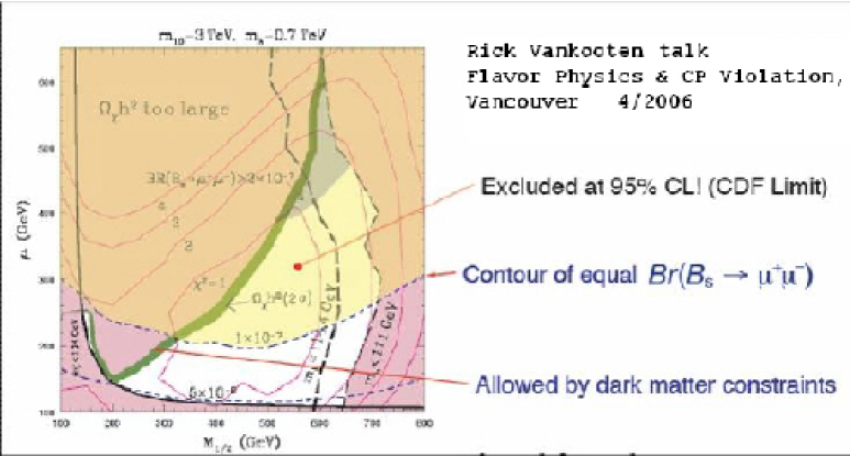
Figure 14: Graph from Ref. [35] with annotations by Rick Vankooten.

3.2 B physics and both the CP odd and light Higgs masses

It is well known that the large $\tan\beta$ region of the MSSM has many interesting consequences for B physics. Let us just consider some interesting examples. We shall consider the branching ratio $Br(B_{s}\rightarrow\mu^{+}\mu^{-})$, the mass splitting $\Delta M_{B_{s}}$, the branching ratio $Br(B_{u}\rightarrow\tau\bar{\nu})$ and the related processes $B\rightarrow X_{s}\gamma$ and $B\rightarrow X_{s}\ l^{+}\ l^{-}$.

3.2.1 $Br(B_{s}\rightarrow\mu^{+}\mu^{-})$

In Fig. 14 we give the contours for the branching ratio $Br(B_{s}\rightarrow\mu^{+}\mu^{-})$ plotted as a function of $\mu$ and $M_{1/2}$ for fixed $m_{16}=3$ TeV and fixed CP odd Higgs mass, $m_{A}=700$ GeV. The most recent ’preliminary’ bounds from CDF [37] and DZero [38] are $Br(B_{s}\rightarrow\mu^{+}\mu^{-})<1.0\times 10^{-7}$ @ 95% CL for CDF with 780 pb^-1 data and $<2.3\times 10^{-7}$ @ 95% CL for DZero with 700 pb^-1 data. Thus only the region below the dashed blue contour $1.0\times 10^{-7}$ is allowed. Note the black dashed vertical contour on the right. This is the light Higgs mass bound. The Higgs mass decreases as $M_{1/2}$ increases.

The amplitude for the process $B_{s}\rightarrow\mu^{+}\mu^{-}$ is dominated by the s-channel CP odd Higgs exchange and the branching ratio scales as $\tan\beta^{6}/m_{A}^{4}$. Thus as $m_{A}$ increases the branching ratio can be made arbitrarily small. On the other hand, we find that as we increase $m_{A}$, we must necessarily increase $M_{1/2}$ in order to satisfy WMAP data. Since in order to have sufficient annihilation we must approximately satisfy $m_{A}\sim 2m_{\chi}$ and $m_{\chi}\propto M_{1/2}$. However, the light Higgs mass decreases as $M_{1/2}$ increases and hence there is an upper bound, $m_{A}(MAX)$, such that WMAP and the light Higgs mass lower bound are both satisfied. We find [35] $m_{A}(MAX)\sim 1.3$ TeV and as a result $Br(B_{s}\rightarrow\mu^{+}\mu^{-})(MIN)\sim 1\times 10^{-8}$ (see Fig. 15).

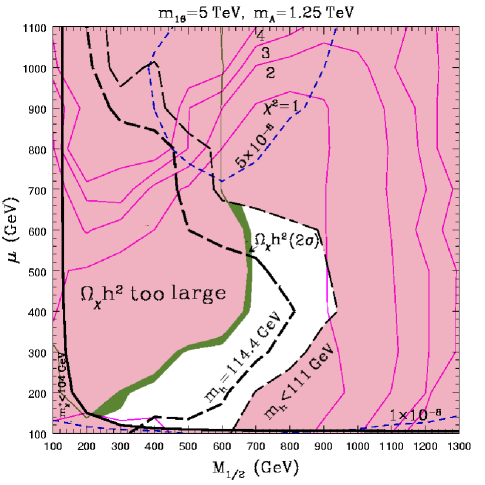
Figure 15: Neutralino abundance and LEP Higgs bound for the CP odd Higgs mass, $m_{A}=1.25$ TeV. Contours of constant $Br(B_{s}\rightarrow\mu^{+}\mu^{-})$ are dashed blue lines.

Thus CDF and DZero have an excellent chance of observing this decay. See Fig. 16.

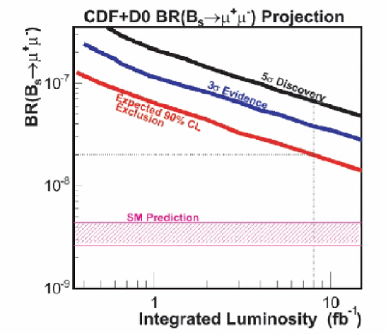
Figure 16: Sensitivity of Fermilab experiments to $Br(B_{s}\rightarrow\mu^{+}\mu^{-})$. Copied from talk by Rick Vankooten at Flavor Physics & CP Violation, Vancouver, April 2006.

3.2.2 Light Higgs mass

It should not be obvious why the light Higgs mass decreases as $M_{1/2}$ increases. This is not a general CMSSM result. In fact this is a consequence of the global $\chi^{2}$ analysis and predominantly constrained by the fit to the bottom quark mass. The bottom quark mass has large SUSY corrections proportional to $\tan\beta$ [39]. The three dominant contributions to these SUSY corrections, $\delta m_{b}/m_{b}$ : a gluino loop contribution $\propto\ \alpha_{3}\ \mu\ M_{\tilde{g}}\ \tan\beta/m_{\tilde{b}_{1}}^{2}$, a chargino loop contribution $\propto\ \lambda_{t}^{2}\ \mu\ A_{t}\ \tan\beta/m_{\tilde{t}_{1}}^{2}$, and a term $\propto\ \log M_{SUSY}^{2}$. In addition, in order to fit $m_{b}(m_{b})$ we need $\delta m_{b}/m_{b}\sim-2$ %. We can now understand why the light Higgs mass decreases as $M_{1/2}$ increases. The gluino and log contribution to the bottom mass correction is positive for $\mu M_{\tilde{g}}$ positive, while the chargino loop contribution is negative, since $A_{t}\sim-M_{\tilde{g}}$ due to an infra-red fixed point in the RG equations. And the sum must be approximately zero (slightly negative). Now, as $M_{1/2}$ increases, the gluino contribution also increases. Then $|A_{t}|$ must also increase. However, the light Higgs mass decreases as $|A_{t}|$ increases (Figs. 17 & 18). For more details, see [35]. In a recent paper we find the light Higgs with mass of order $120\pm 7$ GeV [36].

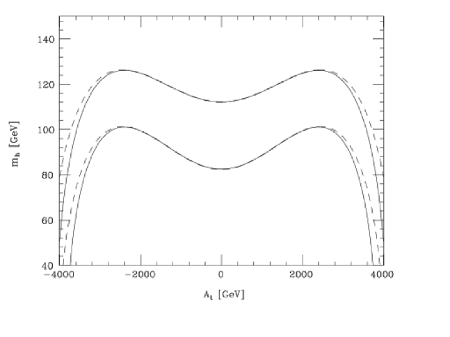
Figure 17: The light Higgs mass as a function of $A_{t}$ for two values of $\tan\beta$ = 1.5 (lower) and 15 (upper) curve [40].

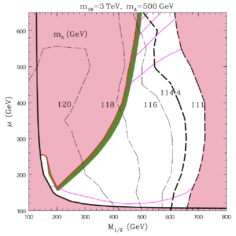
Figure 18: Light Higgs mass contours from Ref. [35]. Note the light Higgs mass obtained here uses the effective field theory formalism [40]. Using FeynHiggs instead, we find values of the light Higgs mass which are of order 3 - 6 GeV larger [36].

3.2.3 $B_{u}\rightarrow\tau\bar{\nu}$

Recently Belle [41] measured the branching ratio $Br(B_{u}\rightarrow\tau\bar{\nu})=1.06\stackrel{{\scriptstyle+0.34}}{{-0.28}}(stat)\stackrel{{\scriptstyle+0.18}}{{-0.16}}(syst)\times 10^{-4}$. The central value is smaller than the expected standard model rate with $R_{B\tau\nu}\equiv\frac{Br^{exp}(B_{u}\rightarrow\tau\bar{\nu})}{Br^{SM}(B_{u}\rightarrow\tau\bar{\nu})}=0.67\stackrel{{\scriptstyle+0.24}}{{-0.21}}_{exp}\pm 0.14_{|f_{B}|}\pm 0.10_{|V_{ub}|}$. Or the central value is $\sim 1\ \sigma$ below the standard model value. This may not be significant, nevertheless this is what is expected in the large $\tan\beta$ limit of the MSSM. As discussed by Isidori and Paradisi [42] (see also, [43]) in the MSSM at large $\tan\beta$ one finds $R_{B\tau\nu}\equiv\frac{Br^{SUSY}(B_{u}\rightarrow\tau\bar{\nu})}{Br^{SM}(B_{u}\rightarrow\tau\bar{\nu})}=\left[1-(\frac{m_{B}^{2}}{m_{H^{\pm}}^{2}})\frac{\tan^{2}\beta}{(1+\epsilon_{0}\tan\beta)}\right]$ where $\epsilon_{0}$ is the result of gluino exchange at one loop. With values of $30<\tan\beta<50$, $0.5<m_{H}/{\rm TeV}<1$ and $\epsilon\sim 10^{-2}$, they find $R_{B\tau\nu}\equiv\frac{Br^{exp}(B_{u}\rightarrow\tau\bar{\nu})}{Br^{SM}(B_{u}\rightarrow\tau\bar{\nu})}=0.67\stackrel{{\scriptstyle+0.30}}{{-0.27}}$, consistent with the data.

3.2.4 $\Delta M_{B_{s}}$

CDF has recently measured the mass splitting $\Delta M_{B_{s}}=17.35\pm 0.25$ ps^-1 [44]. Once again the central value is below the standard model expectation $\Delta M_{B_{s}}=21.5\pm 2.6$ ps^-1 or $R^{exp}_{\Delta M_{s}}\equiv\frac{(\Delta M_{B_{s}})^{exp}}{(\Delta M_{B_{s}})^{SM}}=0.80\pm 0.12$. In SUSY at large $\tan\beta$ one expects [45, 42] $R_{\Delta M_{s}}\equiv\frac{(\Delta M_{B_{s}})^{SUSY}}{(\Delta M_{B_{s}})^{SM}}=1-m_{b}(\mu_{b}^{2})m_{s}(\mu_{b}^{2})\frac{64\pi\sin^{2}\theta_{W}}{\alpha_{em}M_{A}^{2}S_{0}(m_{t}^{2}/M_{W}^{2})}\times\frac{(\epsilon_{Y}\lambda_{t}^{2}\tan^{2}\beta)^{2}}{[1+(\epsilon_{0}+\epsilon_{Y}\lambda_{t}^{2})\tan\beta]^{2}[1+\epsilon\tan\beta]^{2}}$. Hence $\Delta M_{B_{s}}$ is suppressed at large $\tan\beta$.

3.2.5 $B\rightarrow X_{s}\gamma$ and $B\rightarrow X_{s}\ l^{+}\ l^{-}$

The effective Lagrangian for the process $B\rightarrow X_{s}\gamma$ is given by $-L^{eff}\sim C_{7}\ O_{7}$ where $O_{7}=\frac{e}{16\pi^{2}}m_{b}(\bar{s}_{L}\sigma^{\mu\nu}b_{R})F_{\mu\nu}$. In SUSY we have $C_{7}=C_{7}^{SM}+C_{7}^{SUSY}\approx\pm C_{7}^{SM}$ where the second equality is an experimental constraint, since the standard model result fits the data to a reasonable approximation. However at large $\tan\beta$ it was shown that the negative sign is preferred [46].

It is then interesting that the absolute sign of $C_{7}$ is observable in the process $B\rightarrow X_{s}\ l^{+}\ l^{-}$. The effective Lagrangian for this process is given by $-L^{eff}\sim C_{7}O_{7}+C_{9,10}O_{9,10}$ where the latter two operators are electromagnetic penguin diagrams. Gambino et al. [47], using data from Belle and BaBar for $Br(B\rightarrow X_{s}\ l^{+}\ l^{-})$, find $C_{7}=+C_{7}^{SM}$ is preferred. On the other hand, the Belle collaboration [48] analyzed the forward-backward asymmetry for the process $B\rightarrow K^{*}\ l^{+}\ l^{-}$ and find that either sign is acceptable. Clearly this is an important test which must await further data.

3.3 MSO₁₀SM and Large $\tan\beta$

We conclude that the MSO₁₀SM

• fits WMAP;

• predicts light Higgs with mass less than 127 GeV;

• predicts lighter 3rd and heavy 1st & 2nd gen. squarks and sleptons, i.e an inverted scalar mass hierarchy;

• enhances the branching ratio $Br(B_{s}\rightarrow\mu^{+}\mu^{-})$;

• suppresses the branching ratio $Br(B_{u}\rightarrow\tau\bar{\nu})$ and the mass splitting $\Delta M_{B_{s}}$;

• and favors the $sign{C_{7}}=-C_{7}^{SM}$ for the process $B\rightarrow X_{s}\gamma$ which is observable in the decay $B\rightarrow X_{s}\ l^{+}\ l^{-}$.

Clearly the MSO₁₀SM is a beautiful symmetry which has many experimental tests !!

4 Conclusion

Supersymmetric GUTs (defined in 4,5,6 or 10 dimensions) provide a viable, testable and natural extension of the Standard Model. They can also be embedded into string theory, thus defining an ultra-violet completion of such higher dimensional orbifold GUT field theories. Note, that the predictions for nucleon decay are sensitive to whether the theory is defined in four or higher dimensions. Moreover, we showed that the minimal SO(10) SUSY model has a wealth of predictions for low energy experiments. Finally, I would like to thank the organizers for this wonderful workshop.

References

- [1] J. Pati and A. Salam, Phys. Rev. D8 1240 (1973). For more discussion on the standard charge assignments in this formalism, see A. Davidson, Phys. Rev.D20, 776 (1979) and R.N. Mohapatra and R.E. Marshak, Phys. Lett.B91, 222 (1980).
- [2] H. Georgi, Particles and Fields, Proceedings of the APS Div. of Particles and Fields, ed C. Carlson, p. 575 (1975); H. Fritzsch and P. Minkowski, Ann. Phys. 93, 193 (1975).
- [3] H. Georgi and S.L. Glashow, Phys. Rev. Lett. 32 438 (1974).
- [4] H. Georgi, H. Quinn and S. Weinberg, Phys. Rev. Lett. 33 451 (1974); see also the definition of effective field theories by S. Weinberg, Phys. Lett. 91B 51 (1980).
- [5] M. Chanowitz, J. Ellis and M.K. Gaillard, Nucl. Phys. B135, 66 (1978). For the corresponding SUSY analysis, see M. Einhorn and D.R.T. Jones, Nucl. Phys. B196, 475 (1982); K. Inoue, A. Kakuto, H. Komatsu and S. Takeshita, Prog. Theor. Phys. 67, 1889 (1982); L. E. Ibanez and C. Lopez, Phys. Lett. B126, 54 (1983); Nucl. Phys. B233, 511 (1984).
- [6] U. Amaldi, W. de Boer and H. Fürstenau, Phys. Lett. B260, 447 (1991); J. Ellis, S. Kelly and D.V. Nanopoulos, Phys. Lett. B260, 131 (1991); P. Langacker and M. Luo, Phys. Rev. D44, 817 (1991); P. Langacker and N. Polonsky, Phys. Rev. D47, 4028 (1993); M. Carena, S. Pokorski and C.E.M. Wagner, Nucl. Phys. B406, 59 (1993); see also the review by S. Dimopoulos, S. Raby and F. Wilczek, Physics Today, 25–33, October (1991).
- [7] S. Dimopoulos, S. Raby and F. Wilczek, Phys. Rev. D24, 1681 (1981); S. Dimopoulos and H. Georgi, Nucl. Phys. B193, 150 (1981); L. Ibanez and G.G. Ross, Phys. Lett. 105B, 439 (1981); N. Sakai, Z. Phys. C11, 153 (1981); M. B. Einhorn and D. R. T. Jones, Nucl. Phys. B196, 475 (1982); W. J. Marciano and G. Senjanovic, Phys. Rev. D 25, 3092 (1982).
- [8] V. Lucas and S. Raby, Phys. Rev. D54, 2261 (1996) [arXiv:hep-ph/9601303]; T. Blazek, M. Carena, S. Raby and C. E. M. Wagner, Phys. Rev. D56, 6919 (1997) [arXiv:hep-ph/9611217]; G. Altarelli, F. Feruglio and I. Masina, JHEP 0011, 040 (2000) [arXiv:hep-ph/0007254].
- [9] R. Dermíšek, A. Mafi and S. Raby, Phys. Rev. D63, 035001 (2001); K.S. Babu, J.C. Pati and F. Wilczek, Nucl. Phys. B566, 33 (2000).
- [10] M. L. Alciati, F. Feruglio, Y. Lin and A. Varagnolo, JHEP 0503, 054 (2005) [arXiv:hep-ph/0501086].
- [11] Grand Unified Theories, by S. Raby in the Particle Data Group report, W.-M. Yao et al, J. Phys. G 33, 1 (2006).
- [12] K.S. Babu and S.M. Barr, Phys. Rev. D48, 5354 (1993); V. Lucas and S. Raby, Phys. Rev. D54, 2261 (1996); S.M. Barr and S. Raby, Phys. Rev. Lett. 79, 4748 (1997) and references therein.
- [13] G. Altarelli, F. Feruglio, I. Masina, JHEP 0011, 040 (2000). See also earlier papers by A. Masiero, D.V. Nanopoulos, K. Tamvakis and T. Yanagida, Phys. Lett. B115, 380 (1982); B. Grinstein, Nucl. Phys. B206, 387 (1982).
- [14] M. Gell-Mann, P. Ramond and R. Slansky, in Supergravity, ed. P. van Nieuwenhuizen and D.Z. Freedman, North-Holland, Amsterdam, 1979, p. 315.
- [15] S. Weinberg, Phys. Rev. D26, 287 (1982); N. Sakai and T Yanagida, Nucl. Phys. B197, 533 (1982).
- [16] G. Farrar and P. Fayet, Phys. Lett. B76, 575 (1978).
- [17] S. Dimopoulos, S. Raby and F. Wilczek, Phys. Lett. 112B, 133 (1982); J. Ellis, D.V. Nanopoulos and S. Rudaz, Nucl. Phys. B202, 43 (1982).
- [18] See talks by Matthew Earl, NNN workshop, Irvine, February (2000); Y. Totsuka, SUSY2K, CERN, June (2000); Y. Suzuki, International Workshop on Neutrino Oscillations and their Origins, Tokyo, Japan, December (2000) and Baksan School, Baksan Valley, Russia, April (2001), hep-ex/0110005; K. Kobayashi [Super-Kamiokande Collaboration], “Search for nucleon decay from Super-Kamiokande,” Prepared for 27th International Cosmic Ray Conference (ICRC 2001), Hamburg, Germany, 7-15 Aug 2001. For published results see Super-Kamiokande Collaboration: Y. Hayato, M. Earl, et. al, Phys. Rev. Lett. 83, 1529 (1999); K. Kobayashi et al. [Super-Kamiokande Collaboration], [arXiv:hep-ex/0502026].
- [19] T. Goto and T. Nihei, Phys. Rev. D59, 115009 (1999) [arXiv:hep-ph/9808255]; H. Murayama and A. Pierce, Phys. Rev. D65, 055009 (2002) [arXiv:hep-ph/0108104].
- [20] P. Candelas, G.T. Horowitz, A. Strominger, E. Witten, Nucl. Phys. B258, 46 (1985); L.J. Dixon, J.A. Harvey, C. Vafa, E. Witten, Nucl. Phys. B261, 678 (1985), Nucl. Phys. B274, 285 (1986); L. E. Ib a nez, H. P. Nilles, F. Quevedo, Phys. Lett.B187, 25 (1987); L. E. Ib a nez, J. E. Kim, H. P. Nilles, F. Quevedo, Phys. Lett.B191, 282 (1987).
- [21] E. Witten, arXiv:hep-ph/0201018; M. Dine, Y. Nir and Y. Shadmi, Phys. Rev. D66, 115001 (2002) [arXiv:hep-ph/0206268].
- [22] T. Kobayashi, S. Raby, R.-J. Zhang, Phys. Lett. B593, 262 (2004); ibid., Nucl. Phys. B704, 3 (2005).
- [23] S. Förste, H. P. Nilles, P. K. S. Vaudrevange, A. Wingerter, Phys. Rev. D70, 106008 (2004); W. Buchm ller, K. Hamaguchi, O. Lebedev, M. Ratz, Nucl. Phys. B712, 139 (2005); ibid., hep-ph/0512326.
- [24] Y. Kawamura, Progr. Theor. Phys.103, 613 (2000); ibid. 105, 999 (2001); G. Altarelli, F. Feruglio, Phys. Lett.B511, 257 (2001); L. J. Hall, Y. Nomura, Phys. Rev. D64, 055003 (2001); A. Hebecker, J. March-Russell, Nucl. Phys. B613, 3 (2001); T. Asaka, W. Buchm uller, L. Covi, Phys. Lett. B523, 199 (2001); L. J. Hall, Y. Nomura, T. Okui, D. R. Smith, Phys. Rev. D65, 035008 (2002); R. Dermisek and A. Mafi, Phys. Rev. D65, 055002 (2002); H. D. Kim and S. Raby, JHEP 0301, 056 (2003).
- [25] K.R. Dienes, E. Dudas, T. Gherghetta, Phys. Rev. Lett.91, 061601 (2003).
- [26] L. J. Hall, Y. Nomura, Phys. Rev. D64, 055003 (2001).
- [27] L. J. Hall and Y. Nomura, Phys. Rev. D66, 075004 (2002); H. D. Kim, S. Raby and L. Schradin, JHEP 0505, 036 (2005).
- [28] For a recent review see, R. Blumenhagen, M. Cvetic, P. Langacker and G. Shiu, “Toward realistic intersecting D-brane models,” [arXiv:hep-th/0502005].
- [29] G. Aldazabal, A. Font, L. E. Ibanez and A. M. Uranga, Nucl. Phys.B452, 3 (1995); Z. Kakushadze, S.H.H. Tye, Phys. Rev. D54, 7520 (1996); Z. Kakushadze, G. Shiu, S.H.H. Tye, Y. Vtorov-Karevsky, Int. J. Mod. Phys. A13, 2551 (1998).
- [30] G. B. Cleaver, A. E. Faraggi and D. V. Nanopoulos, Int. J. Mod. Phys. A16, 425 (2001) [arXiv:hep-ph/9904301]; G. B. Cleaver, A. E. Faraggi, D. V. Nanopoulos and J. W. Walker, Nucl. Phys. B593, 471 (2001) [arXiv:hep-ph/9910230].
- [31] V. Braun, Y. H. He, B. A. Ovrut and T. Pantev, Phys. Lett. B618, 252 (2005) [arXiv:hep-th/0501070]; V. Braun, Y. H. He, B. A. Ovrut and T. Pantev, JHEP 0506, 039 (2005) [arXiv:hep-th/0502155].
- [32] E. Witten, Nucl. Phys. B471, 135 (1996) [arXiv:hep-th/9602070].
- [33] S. Raby, P. Vaudrevange and A. Wingerter, work in progress.
- [34] T. Blazek, R. Dermisek and S. Raby, Phys. Rev. Lett. 88, 111804 (2002) [arXiv:hep-ph/0107097]; Phys. Rev. D65, 115004 (2002) [arXiv:hep-ph/0201081]; K. Tobe and J. D. Wells, Nucl. Phys. B663, 123 (2003) [arXiv:hep-ph/0301015]; D. Auto, H. Baer, C. Balazs, A. Belyaev, J. Ferrandis and X. Tata, JHEP 0306, 023 (2003) [arXiv:hep-ph/0302155].
- [35] R. Dermisek, S. Raby, L. Roszkowski and R. Ruiz De Austri, JHEP 0304, 037 (2003) [arXiv:hep-ph/0304101]; R. Dermisek, S. Raby, L. Roszkowski and R. Ruiz de Austri, JHEP 0509, 029 (2005) [arXiv:hep-ph/0507233]. [36]
- [36] R. Dermisek, M. Harada and S. Raby, arXiv:hep-ph/0606055.
- [37] See CDF web page: www-cdf.fnal.gov/physics/new/bottom/060316.blessed-bsmumu3/
- [38] See DZero web page: www-d0.fnal.gov/Run2Physics/WWW/results/b.htm
- [39] L.J. Hall, R. Rattazzi and U. Sarid, Phys. Rev. D50, 7048 (1994); M. Carena, M. Olechowski, S. Pokorski and C.E.M. Wagner, Nucl. Phys. B419, 213 (1994); R. Rattazzi and U. Sarid, Nucl. Phys. B501, 297 (1997); T. Blazek, S. Raby and S. Pokorski, Phys. Rev. D 52, 4151 (1995).
- [40] M. Carena, M. Quiros and C. E. M. Wagner, Nucl. Phys. B 461, 407 (1996) [arXiv:hep-ph/9508343].
- [41] K. Ikado et al., arXiv:hep-ex/0604018.
- [42] G. Isidori and P. Paradisi, arXiv:hep-ph/0605012.
- [43] W. S. Hou, Phys. Rev. D 48, 2342 (1993). .
- [44] A. Abulencia [CDF - Run II Collaboration], arXiv:hep-ex/0606027.
- [45] A. J. Buras, P. H. Chankowski, J. Rosiek and L. Slawianowska, Nucl. Phys. B 659 (2003) 3 [hep-ph/0210145]; Phys. Lett. B 546 (2002) 96 [hep-ph/0207241]; Nucl. Phys. B 619 (2001) 434 [hep-ph/0107048].
- [46] T. Blazek and S. Raby, “b s gamma with large tan(beta) in MSSM analysis constrained by a Phys. Rev. D 59, 095002 (1999) [arXiv:hep-ph/9712257].
- [47] P. Gambino, U. Haisch and M. Misiak, Phys. Rev. Lett. 94, 061803 (2005) [arXiv:hep-ph/0410155].
- [48] K. Abe et al. [The Belle Collaboration], “Measurement of forward-backward asymmetry and Wilson coefficients in B arXiv:hep-ex/0508009.