We consider non-canonical embeddings of the MSSM in high-dimensional orbifold GUTs based on the gauge symmetry $SU(N)$, $N=5,6,7,8$. The hypercharge normalization factor $k_{Y}$ can either have unique non-canonical values, such as $23/21$ in a six-dimensional $SU(7)$ model, or may lie in a (continuous) interval. Gauge coupling unification and gauge-Yukawa unification can be realized in these models by introducing new particles with masses in the TeV range which may be found at the LHC. In one such example there exist color singlet fractionally charged states.

1 Introduction

High-dimensional orbifold grand unified theories (GUTs) [1, 2] provide the elegant solutions to the well-known problems encountered in four-dimensional (4D) GUTs such as $SU(5)$ and $SO(10)$, especially the doublet-triplet splitting problem and the proton decay problem. The non-supersymmetric version has, in particular, been exploited to show that unification of the standard model (SM) gauge couplings can be realized with a non-canonical embedding of $U(1)_{Y}$, the hypercharge component of the SM gauge group [3]. The couplings unify at $M_{\rm GUT}\simeq 4\times 10^{16}$ GeV, which is also the scale at which the 4D ${\cal N}=1$ supersymmetry (SUSY) is broken, without introducing additional new particles. This approach has been taken a step further along two different directions. In [4] it was shown that by implementing additional gauge-Yukawa unification, the SM Higgs mass can be predicted. The mass turns out to be $135\pm 6$ ($144\pm 4$) GeV with gauge-top (bottom/tau) Yukawa unification. This is encouraging because it is different from the prediction of $\lesssim 130$ GeV in the minimal supersymmetric standard model (MSSM). In [5] these ideas were extended to the case of split supersymmetry, with similar predictions for the Higgs mass.

The orbifold scenario for the GUT breakings assume the supersymmetric GUT models exist in high dimensions and are broken to 4D ${\cal N}=1$ supersymmetric standard like models for the zero modes due to the discrete symmetries on the extra space manifolds [1, 2]. The zero modes can be identified with the low-energy SM fermions and Higgs fields, allowing gauge-Higgs unification [6] and gauge-Yukawa unification [7]. For the canonical $U(1)_{Y}$ normalization, the unification of the gauge couplings, top and bottom quark Yukawa couplings, and $\tau$ lepton Yukawa coupling can be realized in the 6D orbifold $SU(8)$ and $SU(9)$ models, and cannot be obtained in the orbifold $SU(N)$ models with $N<8$. Therefore, it is interesting to construct the minimal orbifold $SU(N)$ model with gauge-Yukawa unification.

In this paper, we show that the minimal model with the unification of the gauge couplings and third-family Yukawa couplings is the 6D orbifold $SU(7)$ model with non-canonical $U(1)_{Y}$ normalization $k_{Y}=23/21$ where $k_{Y}$ is defined in Eqs. (1) and (2). Moreover, we construct the 7D $SU(8)$ models with gauge-Yukawa unification and $k_{Y}>23/21$. And for completeness, we consider the 6D orbifold $SU(5)$ and $SU(6)$ models with gauge-fermion and gauge-fermion-Higgs unification first as warm up exercise.

The 4D gauge group in these models is $SU(3)_{C}\times SU(2)_{L}\times U(1)_{Y}$ accompanied by one or several extra $U(1)$ factors assumed to be broken at $M_{\rm GUT}$. We define the unified gauge couplings at the GUT scale ($M_{\rm GUT}$) as

$$g_{1}^{2}~{}=~{}g_{2}^{2}~{}=~{}g_{3}^{2}~{},~{}\,$$ (1)

where

$$g_{1}^{2}\equiv k_{Y}g_{Y}^{2}~{},~{}\,$$ (2)

where $k_{Y}$ is the $U(1)_{Y}$ normalization factor, and the $g_{Y}$, $g_{2}$, and $g_{3}$ are the gauge couplings for $U(1)_{Y}$, $SU(2)_{L}$, and $SU(3)_{C}$ gauge groups, respectively. For the canonical $U(1)_{Y}$ normalization, we have $k_{Y}=5/3$.

For orbifold GUTs where all of the SM fermions and Higgs fields are placed on a 3-brane at an orbifold fixed point, we can have any positive normalization for $U(1)_{Y}$, i. e., $k_{Y}$ is an arbitrary positive real number. However, in this case charge quantization cannot be realized. We wish to consider the more interesting orbifold GUTs in which at least one of the SM fermions and Higgs fields arise from the zero modes of the bulk vector multiplet and their $U(1)_{Y}$ charges can be determined. The charge quantization can be achieved due to the gauge invariance of Yukawa couplings and anomaly free conditions. In the orbifold models we consider, $k_{Y}$ is then either uniquely determined to have a non-canonical value or lies in a continuous interval. For the latter case $k_{Y}=5/3$ is possible, but there is no apparent reason why this value would be realized.

Since the three SM gauge couplings unify quite nicely with the canonical hypercharge normalization, it can be argued that we should simply discard the models which do not predict $k_{Y}=5/3$. However, unification in MSSM with $k_{Y}=5/3$ may well be accidental, and as the example of non-supersymmetric unification shows there are different possibilities. In this paper we assume a non-canonical hypercharge normalization as the models under consideration generally predict. We then discuss how gauge coupling unification and gauge-Yukawa unification can be obtained by adding a minimal set of vector-like particles to the MSSM spectrum. It is certainly our hope that these vector-like particles will be found at the Large Hadron Collider (LHC).

The paper is organized as follows. In sections 2 and 3 we consider $SU(5)$ and $SU(6)$ models. In the $SU(5)$ model the only zero mode that can be introduced in the bulk is a quark doublet and $k_{Y}$ is predicted to be $1/15$. The model can be extended to $SU(6)$, with $k_{Y}\geq 1/15$. We construct two $SU(6)$ models with gauge-top and gauge-bottom Yukawa coupling unification, with $k_{Y}=2/3$ and $1/3$ respectively. We discuss $SU(7)$ and $SU(8)$ models in sections 4 and 5. We can have gauge-Yukawa unification for the third family in an $SU(7)$ model, with $k_{Y}=23/21$. This model can be extended to $SU(8)$, with $k_{Y}\geq 23/21$. Sections 6 and 7 concern gauge coupling unification and gauge-Yukawa unification with new particles in these models. We briefly remark on the Higgs mass in section 8 and conclude in section 9. Some details of the 6D and 7D orbifold models are provided in the two appendices.

2 $SU(5)$ Models

We consider a 6D ${\cal N}=(1,1)$ supersymmetric $SU(5)$ gauge theory compactified on the orbifold $M^{4}\times T^{2}/Z_{6}$ (for some details see Appendix A). The ${\cal N}=(1,1)$ supersymmetry in 6D has 16 supercharges and corresponds to ${\cal N}=4$ supersymmetry in 4D, and thus only the gauge multiplet can be introduced in the bulk. This multiplet can be decomposed under the 4D ${\cal N}=1$ supersymmetry into a vector multiplet $V$ and three chiral multiplets $\Sigma_{1}$, $\Sigma_{2}$, and $\Sigma_{3}$ in the adjoint representation, where the fifth and sixth components of the gauge field, $A_{5}$ and $A_{6}$, are contained in the lowest component of $\Sigma_{1}$.

To break the $SU(5)$ gauge symmetry, we choose the following $5\times 5$ matrix representation for $R_{\Gamma_{T}}$,

$$R_{\Gamma_{T}} = {\rm diag}\left(+1,+1,+1,\omega^{n_{1}},\omega^{n_{1}}\right)~{},~{}\,$$ (3)

where $w=e^{{\rm i}\pi/3}$ and $n_{1}\not=0$. Then, we obtain

$$SU(5)/R_{\Gamma_{T}}~{}=~{}SU(3)_{C}\times SU(2)_{L}\times U(1)_{Y}.~{}\,$$ (4)

So, for the zero modes, the 6D ${\cal N}=(1,1)$ supersymmetric $SU(5)$ gauge symmetry is broken down to 4D ${\cal N}=1$ supersymmetric $SU(3)_{C}\times SU(2)_{L}\times U(1)_{Y}$ gauge symmetry [2].

We define the generator for $U(1)_{Y}$ as follows:

$$T_{U(1)_{Y}} \equiv {1\over 30}~{}{\rm diag}\left(2,2,2,-3,-3\right)~{}.~{}\,$$ (5)

Because ${\rm tr}[T_{U(1)_{Y}}^{2}]=1/30$, we obtain $k_{Y}=1/15$.

Under $SU(3)_{C}\times SU(2)_{L}\times U(1)_{Y}$, the adjoint representation $\mathbf{24}$ of $SU(5)$ decomposes as

$$\mathbf{24}=\left(\begin{array}[]{cc}\mathbf{(8,1)}_{Q00}&\mathbf{(3,\bar{2})}_{Q12}\\ \mathbf{(\bar{3},2)}_{Q21}&\mathbf{(1,3)}_{Q00}\end{array}\right)+\mathbf{(1,1)}_{Q_{00}}\,,$$ (6)

where the last term $\mathbf{(1,1)}_{Q_{00}}$ denotes the gauge field associated with $U(1)_{Y}$. The subscripts $Qij$, with $Qij=-Qji$, denote the charges under $U(1)_{Y}$, and

$$Q00~{}=~{}\mathbf{0}~{}~{},~{}Q12=\mathbf{{1\over 6}}~{}.~{}\,$$ (7)

The $Z_{6}$ transformation properties for the decomposed components of $V$, $\Sigma_{1}$, $\Sigma_{2}$, and $\Sigma_{3}$ are given by the first $2\times 2$ submatrices in Eqs. (77)–(80) in Appendix A. We choose

$$k~{}=~{}1~{},~{}~{}n_{1}~{}=~{}5~{},~{}\,$$ (8)

where $k$ is given in Eqs. (75) and (76) in Appendix A. There are no zero modes from the chiral multiplets $\Sigma_{2}$ and $\Sigma_{3}$, and only one zero mode, $\mathbf{(3,\bar{2})}_{Q12}$, from the chiral multiplet $\Sigma_{1}$, which can be identified as the third-family quark doublet $Q_{3}$. The remaining MSSM matter fields and the two MSSM Higgs doublets can be put on the 3-brane at $z=0$, where only the SM gauge symmetry is preserved.

3 $SU(6)$ Models

For the $SU(6)$ models where at least one of the SM fermions and Higgs fields arise from the zero modes of the chiral multiplets $\Sigma_{1}$, $\Sigma_{2}$ and $\Sigma_{3}$, we can show that the minimal normalization $k_{Y}$ for $U(1)_{Y}$ is 1/15, and the corresponding zero mode is quark doublet because it has the smallest $U(1)_{Y}$ quantum number. Moreover, we can only have the gauge-top or gauge-bottom quark Yukawa coupling unification, and we cannot obtain the right-handed leptons from the zero modes of bulk vector multiplet.

In the following subsections, we present three $SU(6)$ models. In the first, the third family quark doublet $Q_{3}$ is the only zero mode from the bulk vector multiplet, and $k_{Y}$ is an arbitrary positive real number that is larger than or equal to 1/15. In the second and third $SU(6)$ models, we have gauge-top and gauge-bottom quark Yukawa coupling unification, respectively. We consider 7D ${\cal N}=1$ supersymmetric $SU(6)$ compactified on the orbifold $M^{4}\times T^{2}/Z_{6}\times S^{1}/Z_{2}$ (for some details see Appendix B), and 6D ${\cal N}=(1,1)$ supersymmetric $SU(6)$ compactified on the orbifold $M^{4}\times T^{2}/Z_{6}$. The compactification process yields 4D ${\cal N}=1$ supersymmetric $SU(3)_{C}\times SU(2)_{L}\times U(1)_{Y}\times U(1)_{\alpha}$.

The generators for $U(1)_{Y}\times U(1)_{\alpha}$ are defined as follows:

$$T_{U(1)_{Y}} \equiv {1\over 30}~{}{\rm diag}\left(2,2,2,-3,-3,0\right)+a~{}{\rm diag}\left(1,1,1,1,1,-5\right),~{}\,$$

$$T_{U(1)_{\alpha}} \equiv ~{}{\rm diag}\left(2,2,2,-3,-3,0\right)-{{1}\over{30a}}~{}{\rm diag}\left(1,1,1,1,1,-5\right),~{}\,$$ (9)

where $a$ is a real number. Because ${\rm tr}[T_{U(1)_{Y}}^{2}]=1/30+30a^{2}$, we obtain

$$k_{Y}~{}=~{}{{1}\over{15}}+60a^{2}~{}\geq~{}{{1}\over{15}}~{}.~{}\,$$ (10)

The adjoint representation $\mathbf{35}$ of $SU(6)$ is decomposed under $SU(3)_{C}\times SU(2)_{L}\times U(1)_{Y}\times U(1)_{\alpha}$ as

$$\mathbf{35}=\left(\begin{array}[]{ccc}\mathbf{(8,1)}_{Q00}&\mathbf{(3,\bar{2})}_{Q12}&\mathbf{(3,1)}_{Q13}\\ \mathbf{(\bar{3},2)}_{Q21}&\mathbf{(1,3)}_{Q00}&\mathbf{(1,2)}_{Q23}\\ \mathbf{(\bar{3},1)}_{Q31}&\mathbf{(1,\bar{2})}_{Q32}&\mathbf{(1,1)}_{Q00}\end{array}\right)+\mathbf{(1,1)}_{Q_{00}}\,,$$ (11)

where $\mathbf{(1,1)}_{Q00}$ in the third diagonal entry of the matrix and the last term $\mathbf{(1,1)}_{Q_{00}}$ denote gauge fields associated with $U(1)_{Y}\times U(1)_{\alpha}$. The subscripts $Qij$, with $Qij=-Qji$, are the charges under $U(1)_{Y}\times U(1)_{\alpha}$. The subscript $Q00~{}=~{}(\mathbf{0},\mathbf{0})$, and the other subscripts $Qij$ with $i\not=j$ are

$$Q12=(\mathbf{{1\over 6}},\mathbf{5})~{},~{}Q13=(\mathbf{{1\over 15}+6a},\mathbf{2-{1\over{5a}}})~{},~{}Q23=(\mathbf{-{1\over 10}+6a},\mathbf{-3-{1\over{5a}}})~{}.~{}$$ (12)

We will consider the following three models.

3.1 $SU(6)$ Model I

Here the third-family quark doublet $Q_{3}$ is the only zero mode from the bulk vector multiplet, $a$ is an arbitrary real number, and we have

$$k_{Y}~{}\geq~{}{{1}\over{15}}~{}.~{}\,$$ (13)

To project out all the unwanted components in the chiral multiplets, we consider the 7D ${\cal N}=1$ supersymmetric $SU(6)$. The ${\cal N}=1$ supersymmetry in 7D has 16 supercharges corresponding to ${\cal N}=4$ supersymmetry in 4D, and only the gauge supermultiplet can be introduced in the bulk. This multiplet can be decomposed under 4D ${\cal N}=1$ supersymmetry into a gauge vector multiplet $V$ and three chiral multiplets $\Sigma_{1}$, $\Sigma_{2}$, and $\Sigma_{3}$ all in the adjoint representation, where the fifth and sixth components of the gauge field, $A_{5}$ and $A_{6}$, are contained in the lowest component of $\Sigma_{1}$, and the seventh component of the gauge field $A_{7}$ is contained in the lowest component of $\Sigma_{2}$.

To break the $SU(6)$ gauge symmetry, we choose the following $6\times 6$ matrix representations for $R_{\Gamma_{T}}$ and $R_{\Gamma_{S}}$

$$R_{\Gamma_{T}} = {\rm diag}\left(+1,+1,+1,\omega^{n_{1}},\omega^{n_{1}},\omega^{n_{2}}\right)~{},~{}\,$$ (14)

$$R_{\Gamma_{S}} = {\rm diag}\left(+1,+1,+1,+1,+1,+1\right)~{},~{}\,$$ (15)

where $n_{1}\not=n_{2}\not=0$.

Then, we obtain

$$SU(6)/R_{\Gamma_{T}}~{}=~{}SU(3)\times SU(2)\times U(1)_{Y}\times U(1)_{\alpha}~{},~{}\,$$ (16)

$$SU(6)/R_{\Gamma_{S}}~{}=~{}SU(6)~{},~{}\,$$ (17)

$$SU(6)/\{R_{\Gamma_{T}}\cup R_{\Gamma_{S}}\}~{}=~{}SU(3)\times SU(2)\times U(1)_{Y}\times U(1)_{\alpha}~{}.~{}\,$$ (18)

Note that $R_{\Gamma_{S}}$ only breaks the additional supersymmetry.

The $Z_{6}\times Z_{2}$ transformation properties for the decomposed components of $V$, $\Sigma_{1}$, $\Sigma_{2}$, and $\Sigma_{3}$ are the $3\times 3$ submatrices in Eqs. (92)–(95) in Appendix B where the third and fourth rows and columns are crossed out. We choose

$$n_{1}~{}=~{}5~{},~{}~{}n_{2}~{}=~{}2~{}~{}{\rm or}~{}~{}3~{}.~{}\,$$ (19)

Then, we obtain that there is no zero mode from the chiral multiplets $\Sigma_{2}$ and $\Sigma_{3}$, and only one zero mode, $\mathbf{(3,\bar{2})}_{Q12}$, from the chiral multiplet $\Sigma_{1}$, which can be identified with the third-family quark doublet $Q_{3}$.

3.2 $SU(6)$ Model II and $SU(6)$ Model III

In this subsection, we will construct $SU(6)$ models with gauge-top and gauge-bottom quark Yukawa coupling unification. We consider 6D ${\cal N}=(1,1)$ supersymmetric $SU(6)$ compactified on the orbifold $M^{4}\times T^{2}/Z_{6}$. To break the $SU(6)$ gauge symmetry, we choose the following $6\times 6$ matrix representation for $R_{\Gamma_{T}}$

$$R_{\Gamma_{T}} = {\rm diag}\left(+1,+1,+1,\omega^{n_{1}},\omega^{n_{1}},\omega^{n_{2}}\right)~{},~{}\,$$ (20)

where $n_{1}\not=n_{2}\not=0$. Then, we obtain

$$SU(6)/R_{\Gamma_{T}}~{}=~{}SU(3)_{C}\times SU(2)_{L}\times U(1)_{Y}\times U(1)_{\alpha}.~{}\,$$ (21)

The $Z_{6}$ transformation properties for the decomposed components of $V$, $\Sigma_{1}$, $\Sigma_{2}$, and $\Sigma_{3}$ are given by the first $3\times 3$ submatrices in Eqs. (77)–(80) in Appendix A. We choose

$$k~{}=~{}1~{},~{}~{}n_{1}~{}=~{}5~{},~{}~{}n_{2}~{}=~{}2~{},~{}\,$$ (22)

and consider the following two models:

(A) $SU(6)$ Model II (gauge-top quark Yukawa coupling unification)

With

$$a~{}=~{}{1\over{10}}~{},~{}\,$$ (23)

we have

$$k_{Y}~{}=~{}{2\over 3}~{}.~{}\,$$ (24)

The zero modes from the chiral multiplets $\Sigma_{1}$, $\Sigma_{2}$ and $\Sigma_{3}$ are presented in Table 1. We can identify them as the third-family quark doublet, the right-handed top quark, and the MSSM Higgs doublets.

Chiral Fields	Zero Modes
$\Sigma_{1}$	$Q_{3}$:  $\mathbf{(3,\bar{2})}_{Q12}$
$\Sigma_{2}$	$t^{c}$:  $\mathbf{(\bar{3},1)}_{Q31}$
$\Sigma_{3}$	$H_{u}$:  $\mathbf{(1,2)}_{Q23}$;  $H_{d}$:  $\mathbf{(1,\bar{2})}_{Q32}$

Table 1: Zero modes from the chiral multiplets $\Sigma_{1}$, $\Sigma_{2}$ and $\Sigma_{3}$ in $SU(6)$ (Model II).

From the trilinear term in the 6D bulk action, we obtain the top quark Yukawa term

$$\int d^{6}x\left[\int d^{2}\theta\ g_{6}Q_{3}t^{c}H_{u}+h.c.\right]~{}.~{}\,$$ (25)

Thus, at $M_{\rm GUT}$, we have

$$g_{1}=g_{2}=g_{3}=y_{t}=g_{6}/\sqrt{V}~{},~{}\,$$ (26)

where $y_{t}$ is the top quark Yukawa coupling, and $V$ is the physical volume of extra dimensions.

(B) $SU(6)$ Model III (gauge-bottom quark Yukawa coupling unification)

For this case we set

$$a~{}=~{}-{1\over{15}}~{},~{}\,$$ (27)

in which case

$$k_{Y}~{}=~{}{1\over 3}~{}.~{}\,$$ (28)

The zero modes arise from the chiral multiplets $\Sigma_{1}$, $\Sigma_{2}$ and $\Sigma_{3}$, and are presented in Table 2. We can identify them as the third-family quark doublet, the right-handed bottom quark, and the MSSM Higgs doublets.

Chiral Fields	Zero Modes
$\Sigma_{1}$	$Q_{3}$:  $\mathbf{(3,\bar{2})}_{Q12}$
$\Sigma_{2}$	$b^{c}$:  $\mathbf{(\bar{3},1)}_{Q31}$
$\Sigma_{3}$	$H_{d}$:  $\mathbf{(1,2)}_{Q23}$;  $H_{u}$:  $\mathbf{(1,\bar{2})}_{Q32}$

Table 2: Zero modes from the chiral multiplets $\Sigma_{1}$, $\Sigma_{2}$ and $\Sigma_{3}$ in $SU(6)$ (Model III).

From the trilinear term in the 6D bulk action, we obtain the bottom quark Yukawa term

$$\int d^{6}x\left[\int d^{2}\theta\ g_{6}Q_{3}b^{c}H_{d}+h.c.\right]~{}.~{}\,$$ (29)

Thus, at $M_{\rm GUT}$, we have

$$g_{1}=g_{2}=g_{3}=y_{b}=g_{6}/\sqrt{V}~{},~{}\,$$ (30)

where $y_{b}$ is the bottom quark Yukawa coupling.

4 $SU(7)$ Models

As we discussed above, to achieve gauge-fermion-Higgs unification, the minimal gauge group is $SU(7)$, with $U(1)_{Y}$ normalization $k_{Y}=23/21$ which is uniquely determined. This can be seen as follows. The $U(1)_{Y}$ generator in $SU(7)$ belongs to its Cartan subalgebra, and can be parametrized as

$$T_{U(1)_{Y}}\equiv{\rm diag}\left(r_{3},r_{3},r_{3},r_{2},r_{2},r_{1},r^{\prime}_{1}\right)~{}.~{}$$ (31)

The traceless condition yields

$$3r_{3}+2r_{2}+r_{1}+r^{\prime}_{1}~{}=~{}0~{},~{}\,$$ (32)

and gauge-fermion-Higgs unification requires that

$$r_{3}-r_{2}~{}=~{}{1\over 6}~{},~{}~{}r_{3}-r_{1}~{}=~{}{2\over 3}~{},~{}~{}r_{3}-r^{\prime}_{1}~{}=~{}-{1\over 3}~{}.~{}\,$$ (33)

Thus, we have the unique solution

$$r_{3}~{}=~{}{{2}\over{21}}~{},~{}~{}r_{2}~{}=~{}-{{1}\over{14}}~{},~{}~{}r_{1}~{}=~{}-{{4}\over{7}}~{},~{}r^{\prime}_{1}~{}=~{}{{3}\over{7}}~{},~{}\,$$ (34)

for which ${\rm tr}[T_{U(1)_{Y}}^{2}]=23/42$. With a canonical normalization ${\rm tr}[T_{i}^{2}]=1/2$ of non-abelian generators, we obtain $k_{Y}=23/21$.

We consider a 6D ${\cal N}=(1,1)$ supersymmetric $SU(7)$ gauge theory compactified on the orbifold $M^{4}\times T^{2}/Z_{6}$ (for some details see Appendix A). To break $SU(7)$, we select the following $7\times 7$ matrix representation for $R_{\Gamma_{T}}$

$$R_{\Gamma_{T}} = {\rm diag}\left(+1,+1,+1,\omega^{n_{1}},\omega^{n_{1}},\omega^{n_{2}},\omega^{n_{3}}\right)~{},~{}\,$$ (35)

where $n_{1}\not=n_{2}\not=n_{3}\not=0$. Thus,

$$SU(7)/R_{\Gamma_{T}}~{}=~{}SU(3)_{C}\times SU(2)_{L}\times U(1)_{Y}\times U(1)_{\beta}\times U(1)_{\gamma}~{}.~{}\,$$ (36)

So, for the zero modes, the 6D ${\cal N}=(1,1)$ supersymmetric $SU(7)$ gauge symmetry is broken down to 4D ${\cal N}=1$ supersymmetric $SU(3)_{C}\times SU(2)_{L}\times U(1)_{Y}\times U(1)_{\beta}\times U(1)_{\gamma}$ gauge symmetry [2]. We assume that the two additional $U(1)$ symmetries can be spontaneously broken at $M_{\rm GUT}$ by the usual Higgs mechanism. It is conceivable that these two symmetries can play some useful role as flavor symmetries [8], but we will not pursue this any further here.

We define the generators for the $U(1)_{Y}\times U(1)_{\beta}\times U(1)_{\gamma}$ gauge symmetry as follows

$$T_{U(1)_{Y}} \equiv {1\over 42}~{}{\rm diag}\left(4,4,4,-3,-3,-24,18\right)~{},~{}\,$$

$$T_{U(1)_{\beta}} \equiv {\rm diag}\left(1,1,1,0,0,-1,-2\right),~{}\,$$

$$T_{U(1)_{\gamma}} \equiv {\rm diag}\left(3,3,3,-8,-8,5,2\right).~{}\,$$ (37)

The $SU(7)$ adjoint representation $\mathbf{48}$ decomposes under the $SU(3)_{C}\times SU(2)_{L}\times U(1)_{Y}\times U(1)_{\beta}\times U(1)_{\gamma}$ gauge symmetry as

$$\mathbf{48}=\left(\begin{array}[]{cccc}\mathbf{(8,1)}_{Q00}&\mathbf{(3,\bar{2})}_{Q12}&\mathbf{(3,1)}_{Q13}&\mathbf{(3,1)}_{Q14}\\ \mathbf{(\bar{3},2)}_{Q21}&\mathbf{(1,3)}_{Q00}&\mathbf{(1,2)}_{Q23}&\mathbf{(1,2)}_{Q24}\\ \mathbf{(\bar{3},1)}_{Q31}&\mathbf{(1,\bar{2})}_{Q32}&\mathbf{(1,1)}_{Q00}&\mathbf{(1,1)}_{Q34}\\ \mathbf{(\bar{3},1)}_{Q41}&\mathbf{(1,\bar{2})}_{Q42}&\mathbf{(1,1)}_{Q43}&\mathbf{(1,1)}_{Q00}\end{array}\right)+\mathbf{(1,1)}_{Q_{00}}\,,$$ (38)

where $\mathbf{(1,1)}_{Q00}$ in the third and fourth diagonal entries of the matrix and the last term $\mathbf{(1,1)}_{Q_{00}}$ denote the gauge fields associated with $U(1)_{Y}\times U(1)_{\beta}\times U(1)_{\gamma}$. The subscripts $Qij$, which are anti-symmetric ($Qij=-Qji$), are the charges under $U(1)_{Y}\times U(1)_{\beta}\times U(1)_{\gamma}$. The subscript $Q00~{}=~{}(\mathbf{0},\mathbf{0},\mathbf{0})$, and the other subscripts $Qij$ with $i\not=j$ are

$$Q12=(\mathbf{{1\over 6}},\mathbf{1},\mathbf{11})~{},~{}Q13=(\mathbf{2\over 3},\mathbf{2},\mathbf{-2})~{},~{}$$

$$Q14=(\mathbf{-{1\over 3}},\mathbf{3},\mathbf{1})~{},~{}Q23=(\mathbf{1\over 2},\mathbf{1},\mathbf{-13})~{},~{}$$

$$Q24=(\mathbf{-{1\over 2}},\mathbf{2},\mathbf{-10})~{},~{}Q34=(\mathbf{-1},\mathbf{1},\mathbf{3})~{}.~{}\,$$ (39)

The $Z_{6}$ transformation properties for the decomposed components of $V$, $\Sigma_{1}$, $\Sigma_{2}$, and $\Sigma_{3}$ are given by Eqs. (77)–(80). We will consider two concrete models.

4.1 $SU(7)$ Model I

We choose

$$k~{}=~{}1~{},~{}~{}n_{1}~{}=~{}4~{},~{}~{}n_{2}~{}=~{}1~{},~{}~{}n_{3}~{}=~{}2~{},~{}\,$$ (40)

where $k$ is given in Eqs. (75) and (76) in Appendix A. The zero modes from the chiral multiplets $\Sigma_{1}$, $\Sigma_{2}$ and $\Sigma_{3}$ are presented in Table 3. We can identify them as the third-family SM fermions, and one pair of Higgs doublets. Interestingly, we do not have any exotic particle from the zero modes of the chiral multiplets.

Chiral Fields	Zero Modes
$\Sigma_{1}$	$t^{c}$: $\mathbf{(\bar{3},1)}_{Q31}$;  $\tau^{c}$:  $\mathbf{(1,1)}_{Q43}$
$\Sigma_{2}$	$Q_{3}$:  $\mathbf{(3,\bar{2})}_{Q12}$;  $H_{d}$:  $\mathbf{(1,2)}_{Q24}$;  $b^{c}$:  $\mathbf{(\bar{3},1)}_{Q41}$
$\Sigma_{3}$	$H_{u}$:  $\mathbf{(1,2)}_{Q23}$;  $L_{3}$:  $\mathbf{(1,\bar{2})}_{Q32}$

Table 3: Zero modes from the chiral multiplets $\Sigma_{1}$, $\Sigma_{2}$ and $\Sigma_{3}$ in $SU(7)$ (Model I).

From the trilinear term in the 6D bulk action, we obtain the top quark and tau lepton Yukawa terms

$$\int d^{6}x\left[\int d^{2}\theta\ g_{7}\left(Q_{3}t^{c}H_{u}+L_{3}\tau^{c}H_{d}\right)+h.c.\right]~{}.~{}\,$$ (41)

Thus, at $M_{\rm GUT}$, we have

$$g_{1}=g_{2}=g_{3}=y_{t}=y_{\tau}=g_{7}/\sqrt{V}~{},~{}\,$$ (42)

where $y_{\tau}$ is the tau lepton Yukawa coupling. However, we do not have the bottom quark Yukawa term from 6D bulk action.

4.2 $SU(7)$ Model II

We choose

$$k~{}=~{}1~{},~{}~{}n_{1}~{}=~{}4~{},~{}~{}n_{2}~{}=~{}1~{},~{}~{}n_{3}~{}=~{}3~{}.~{}\,$$ (43)

The zero modes from the chiral multiplets $\Sigma_{1}$, $\Sigma_{2}$ and $\Sigma_{3}$ are given in Table 4. We can identify them as the third-family SM fermions, the MSSM Higgs doublets, and an exotic (left-handed singlet) quark $b_{X}$.

Chiral Fields	Zero Modes
$\Sigma_{1}$	$H_{d}$:  $\mathbf{(1,2)}_{Q24}$;  $t^{c}$: $\mathbf{(\bar{3},1)}_{Q31}$
$\Sigma_{2}$	$Q_{3}$:  $\mathbf{(3,\bar{2})}_{Q12}$;  $\tau^{c}$:  $\mathbf{(1,1)}_{Q43}$
$\Sigma_{3}$	$H_{u}$:  $\mathbf{(1,2)}_{Q23}$;  $L_{3}$:  $\mathbf{(1,\bar{2})}_{Q32}$;  $b^{c}$:  $\mathbf{(\bar{3},1)}_{Q41}$;  $b_{X}$:  $\mathbf{(3,1)}_{Q14}$

Table 4: Zero modes from the chiral multiplets $\Sigma_{1}$, $\Sigma_{2}$ and $\Sigma_{3}$ in the $SU(7)$ Model II.

From the trilinear term in the 6D bulk action, we obtain the top quark, bottom quark, and tau lepton Yukawa terms

$$\int d^{6}x\left[\int d^{2}\theta\ g_{7}\left(Q_{3}t^{c}H_{u}+Q_{3}b^{c}H_{d}+L_{3}\tau^{c}H_{d}\right)+h.c.\right].~{}\,$$ (44)

Thus, at $M_{\rm GUT}$, we have

$$g_{1}=g_{2}=g_{3}=y_{t}=y_{b}=y_{\tau}=g_{7}/\sqrt{V}~{}.~{}\,$$ (45)

Thus, we have unification of the SM gauge couplings and the third-family SM fermion Yukawa couplings.

We can give GUT-scale mass to the exotic quark $b_{X}$ by introducing an additional exotic quark ${\bar{b}}_{X}$ with quantum number $\mathbf{(\bar{3},1)}_{QX}$ on the observable 3-brane at $z=0$, where $QX=(\mathbf{{1\over 3},\mathbf{-3},\mathbf{0}})$. Suppose we introduce one pair of SM singlets $S^{\prime}$ and $\overline{S^{\prime}}$ with charges $\mathbf{1}$ and $\mathbf{-1}$ respectively whose VEVs break $U(1)_{\gamma}$ at $M_{\rm GUT}$. The exotic quarks $b_{X}$ and ${\bar{b}}_{X}$ can pair up and acquire $M_{\rm GUT}$ mass via the brane-localized superpotential term $\overline{S^{\prime}}b_{X}{\bar{b}}_{X}$.

5 $SU(8)$ Models

We are unable to construct orbifold models of gauge-fermion-Higgs unification with $k_{Y}<23/21$. To construct models with $k_{Y}\geq 23/21$, we consider a 7D ${\cal N}=1$ supersymmetric $SU(8)$ gauge theory compactified on the orbifold $M^{4}\times T^{2}/Z_{6}\times S^{1}/Z_{2}$ (for some details see Appendix B). To break the $SU(8)$ gauge symmetry, we choose the following $8\times 8$ matrix representations for $R_{\Gamma_{T}}$ and $R_{\Gamma_{S}}$

$$R_{\Gamma_{T}} = {\rm diag}\left(+1,+1,+1,\omega^{n_{1}},\omega^{n_{1}},\omega^{n_{1}},+1,\omega^{n_{2}}\right)~{},~{}\,$$ (46)

$$R_{\Gamma_{S}} = {\rm diag}\left(+1,+1,+1,+1,+1,-1,-1,+1\right)~{},~{}\,$$ (47)

where $n_{1}\not=n_{2}\not=0$. We obtain

$$SU(8)/R_{\Gamma_{T}}~{}=~{}SU(4)\times SU(3)\times U(1)^{2}~{},~{}\,$$ (48)

$$SU(8)/R_{\Gamma_{S}}~{}=~{}SU(6)\times SU(2)\times U(1)~{},~{}\,$$ (49)

$$SU(8)/\{R_{\Gamma_{T}}\cup R_{\Gamma_{S}}\}~{}=~{}SU(3)_{C}\times SU(2)_{L}\times U(1)_{Y}\times U(1)_{\alpha}\times U(1)_{\beta}\times U(1)_{\gamma}~{}.~{}\,$$ (50)

Thus, for the zero modes, the 7D ${\cal N}=1$ supersymmetric $SU(8)$ gauge symmetry is broken down to a 4D ${\cal N}=1$ supersymmetric $SU(3)_{C}\times SU(2)_{L}\times U(1)_{Y}\times U(1)_{\alpha}\times U(1)_{\beta}\times U(1)_{\gamma}$ gauge symmetry [2].

We define the generators for the $U(1)_{Y}\times U(1)_{\alpha}\times U(1)_{\beta}\times U(1)_{\gamma}$ gauge symmetry as follows:

$$T_{U(1)_{Y}} \equiv {1\over 42}~{}{\rm diag}\left(4,4,4,-3,-3,-24,18,0\right)+a~{}{\rm diag}\left(1,1,1,1,1,1,1,-7\right),~{}\,$$

$$T_{U(1)_{\alpha}} \equiv ~{}{\rm diag}\left(4,4,4,-3,-3,-24,18,0\right)-{{23}\over{56a}}~{}{\rm diag}\left(1,1,1,1,1,1,1,-7\right),~{}\,$$

$$T_{U(1)_{\beta}} \equiv {\rm diag}\left(1,1,1,0,0,-1,-2,0\right),~{}\,$$

$$T_{U(1)_{\gamma}} \equiv {\rm diag}\left(3,3,3,-8,-8,5,2,0\right),~{}\,$$ (51)

where $a$ is a real number. Because ${\rm tr}[T_{U(1)_{Y}}^{2}]=23/42+56a^{2}$, we obtain

$$k_{Y}~{}=~{}{{23}\over{21}}+112a^{2}~{}\geq~{}{{23}\over{21}}~{}.~{}\,$$ (52)

Incidentally, for the canonical $U(1)_{Y}$ normalization ($k_{Y}=5/3$), we have $a=1/14$, and $U(1)_{Y}$ coincides with $U(1)_{Y}$ in the Pati-Salam or Pati-Salam like models when we break $SU(8)$ down to $SU(4)_{C}\times SU(2)_{L}\times SU(2)_{R}\times U(1)^{2}$ or $SU(3)_{C}\times SU(2)_{L}\times U(1)_{B-L}\times U(1)_{I_{3R}}\times U(1)^{2}$ by orbifold projections.

The $SU(8)$ adjoint representation $\mathbf{63}$ decomposes under $SU(3)_{C}\times SU(2)_{L}\times U(1)_{Y}\times U(1)_{\alpha}\times U(1)_{\beta}\times U(1)_{\gamma}$ gauge symmetry as:

$$\mathbf{63}=\left(\begin{array}[]{ccccc}\mathbf{(8,1)}_{Q00}&\mathbf{(3,\bar{2})}_{Q12}&\mathbf{(3,1)}_{Q13}&\mathbf{(3,1)}_{Q14}&\mathbf{(3,1)}_{Q15}\\ \mathbf{(\bar{3},2)}_{Q21}&\mathbf{(1,3)}_{Q00}&\mathbf{(1,2)}_{Q23}&\mathbf{(1,2)}_{Q24}&\mathbf{(1,2)}_{Q25}\\ \mathbf{(\bar{3},1)}_{Q31}&\mathbf{(1,\bar{2})}_{Q32}&\mathbf{(1,1)}_{Q00}&\mathbf{(1,1)}_{Q34}&\mathbf{(1,1)}_{Q35}\\ \mathbf{(\bar{3},1)}_{Q41}&\mathbf{(1,\bar{2})}_{Q42}&\mathbf{(1,1)}_{Q43}&\mathbf{(1,1)}_{Q00}&\mathbf{(1,1)}_{Q45}\\ \mathbf{(\bar{3},1)}_{Q51}&\mathbf{(1,\bar{2})}_{Q52}&\mathbf{(1,1)}_{Q53}&\mathbf{(1,1)}_{Q54}&\mathbf{(1,1)}_{Q00}\end{array}\right)+\mathbf{(1,1)}_{Q00}~{},~{}\,$$ (53)

where $\mathbf{(1,1)}_{Q00}$ in the third, fourth and fifth diagonal entries of the matrix, and the last term $\mathbf{(1,1)}_{Q00}$ denote the gauge fields for $U(1)_{Y}\times U(1)_{\alpha}\times U(1)_{\beta}\times U(1)_{\gamma}$. Moreover, the subscripts $Qij$, with $Qij=-Qji$, are the charges under $U(1)_{Y}\times U(1)_{\alpha}\times U(1)_{\beta}\times U(1)_{\gamma}$. The subscript $Q00~{}=~{}(\mathbf{0},\mathbf{0},\mathbf{0},\mathbf{0})$, and the other subscripts $Qij$ with $i\not=j$ are

$$Q12=(\mathbf{{1\over 6}},\mathbf{7},\mathbf{1},\mathbf{11})~{},~{}Q13=(\mathbf{2\over 3},\mathbf{28},\mathbf{2},\mathbf{-2})~{},~{}$$

$$Q14=(\mathbf{-{1\over 3}},\mathbf{-14},\mathbf{3},\mathbf{1})~{},~{}Q23=(\mathbf{1\over 2},\mathbf{21},\mathbf{1},\mathbf{-13})~{},~{}$$

$$Q24=(\mathbf{-{1\over 2}},\mathbf{-21},\mathbf{2},\mathbf{-10})~{},~{}Q34=(\mathbf{-1},\mathbf{-42},\mathbf{1},\mathbf{3})~{},~{}$$

$$Q15=\left(\mathbf{{2\over{21}}+8a},\mathbf{4-{{23}\over{7a}}},\mathbf{1},\mathbf{3}\right)~{},$$

$$Q25=\left(\mathbf{-{1\over{14}}+8a},\mathbf{-3-{{23}\over{7a}}},\mathbf{0},\mathbf{-8}\right)~{},$$

$$Q35=\left(\mathbf{-{4\over{7}}+8a},\mathbf{-24-{{23}\over{7a}}},\mathbf{-1},\mathbf{5}\right)~{},$$

$$Q45=\left(\mathbf{{3\over{7}}+8a},\mathbf{18-{{23}\over{7a}}},\mathbf{-2},\mathbf{2}\right)~{}.$$ (54)

The $Z_{6}\times Z_{2}$ transformation properties for the decomposed components of $V$, $\Sigma_{1}$, $\Sigma_{2}$, and $\Sigma_{3}$ are given by Eqs. (92)–(95) in Appendix B. And we choose

$$n_{1}~{}=~{}5~{},~{}~{}n_{2}~{}=~{}2~{}~{}{\rm or}~{}~{}3~{}.~{}\,$$ (55)

The zero modes from the chiral multiplets $\Sigma_{1}$, $\Sigma_{2}$ and $\Sigma_{3}$ are presented in Table 5. We can identify them as the third-family SM fermions, the MSSM Higgs doublets, and the exotic quark $b_{X}$.

Chiral Fields	Zero Modes
$\Sigma_{1}$	$Q_{3}$:  $\mathbf{(3,\bar{2})}_{Q12}$;  $\tau^{c}$:  $\mathbf{(1,1)}_{Q43}$
$\Sigma_{2}$	$H_{u}$:  $\mathbf{(1,2)}_{Q23}$;  $L_{3}$:  $\mathbf{(1,\bar{2})}_{Q32}$;  $b^{c}$:  $\mathbf{(\bar{3},1)}_{Q41}$;  $b_{X}$:  $\mathbf{(3,1)}_{Q14}$
$\Sigma_{3}$	$H_{d}$:  $\mathbf{(1,2)}_{Q24}$;  $t^{c}$: $\mathbf{(\bar{3},1)}_{Q31}$

Table 5: Zero modes from the chiral multiplets $\Sigma_{1}$, $\Sigma_{2}$ and $\Sigma_{3}$ in the $SU(8)$ model.

From the trilinear term in the 7D bulk action, we obtain the top quark, bottom quark, and tau lepton Yukawa terms

$$\int d^{7}x\left[\int d^{2}\theta\ g_{8}\left(Q_{3}t^{c}H_{u}+Q_{3}b^{c}H_{d}+L_{3}\tau^{c}H_{d}\right)+h.c.\right].~{}\,$$ (56)

Thus, at $M_{\rm GUT}$, we have

$$g_{1}=g_{2}=g_{3}=y_{t}=y_{b}=y_{\tau}=g_{8}/\sqrt{V}~{}.~{}\,$$ (57)

6 New Particles and Gauge Coupling Unification

For non-canonical $U(1)_{Y}$ normalization, it is necessary to introduce new particles to achieve unification. Here, as an example, we consider restoring gauge coupling unification by adding a minimal set of vector-like particles with SM quantum numbers. These particles can be put on the 3-brane at $z=0$, and their masses can be the order of the weak scale due to the Giudice-Masiero mechanism [9].

We denote these particles as $u_{x}$ and so on, where $u_{x}$ stands for the vector-like pair with the same quantum numbers as these for $u+u^{c}$. Although we employ two-loop renormalization group equations (RGEs) for the gauge couplings in the numerical calculations, for the discussions below we will consider one-loop $\beta$-coefficients which, for the MSSM and vector-like particles, are as follows:

$$b_{\rm MSSM}=\left(\frac{11}{k_{Y}},1,-3\right), b_{Q_{x}}=\left(\frac{1}{3k_{Y}},3,2\right),$$

$$b_{u_{x}}=\left(\frac{8}{3k_{Y}},0,1\right), b_{d_{x}}=\left(\frac{2}{3k_{Y}},0,1\right),$$

$$b_{L_{x}}=\left(\frac{1}{k_{Y}},1,0\right), b_{e_{x}}=\left(\frac{2}{k_{Y}},0,0\right)\,.$$ (58)

From the one-loop RGEs, it is straightforward to obtain the following relations:

$$\log\frac{M_{\rm GUT}}{m_{Z}} = \frac{2\pi(\alpha_{s}^{-1}\alpha-s^{2}_{W})}{\alpha(b_{3}-b_{2})}\,,$$ (59)

$$\alpha_{s}^{-1} = \left[s^{2}_{W}+\frac{1-(1+k_{Y})s^{2}_{W}}{k_{Y}}\left(\frac{b_{3}-b_{2}}{b_{1}-b_{2}}\right)\right]\alpha^{-1}\,,$$ (60)

$$\alpha_{\rm GUT} = \frac{k_{Y}\alpha(b_{1}-b_{2})}{k_{Y}s^{2}_{W}b_{1}-(1-s^{2}_{W})b_{2}}\,,$$ (61)

where $s_{W}$ stands for $\sin\theta_{W}$, and $\alpha$ and $\alpha_{s}$ are the electromagnetic and strong couplings at $m_{Z}$. From Eq. (58), we see that $b_{3}-b_{2}$ is an integer. For the GUT scale to be smaller than the Planck scale and large enough to avoid the bounds on proton decay, Eq. (59) requires the contribution $(b_{3}-b_{2})_{x}$ from vector-like particles to vanish, assuming the latter have masses close to the weak scale. From Eq. (60), the range of $(b_{1}-b_{2})_{x}$ allowing gauge coupling unification can be obtained depending on the value of $k_{Y}$. Also, $\alpha_{\rm GUT}\ll 1$ is required for perturbative unification.

Simple examples that satisfy the above conditions are as follows. For $k_{Y}=1/15$ as in the $SU(5)$ model, gauge coupling unification can be restored by adding two sets of $L_{x}+u_{x}$. Unification can also be restored by adding $L_{x}+u_{x}+2e_{x}$ or by adding $4e_{x}$. For $k_{Y}=1/3$ as in the $SU(6)$ model with gauge-bottom quark Yukawa coupling unification, one can again add two sets of $L_{x}+u_{x}$, or $3e_{x}$. And for $k_{Y}=2/3$ as in the $SU(6)$ model with gauge-top quark Yukawa coupling unification, one can add $L_{x}+u_{x}+e_{x}$ or $3(L_{x}+d_{x})+e_{x}$. Finally, for $k_{Y}=23/21$ as in the $SU(7)$ model with the unification of the gauge couplings and third-family Yukawa couplings, one can add $L_{x}+u_{x}$. Because such additional vector-like particles can be observed at the LHC and ILC, we can distinguish these models with these future experiments.

7 New Particles and Gauge-Yukawa Unification

In this section we probe gauge-Yukawa unification following the analysis in Ref. [10] (see also Ref. [11] for details and references). In our analysis, we use a dimensional reduction ($\overline{\rm DR}$) renormalization scheme, which is known to be consistent with SUSY. ${\overline{\rm{DR}}}$ Yukawa couplings ($y_{t,b,\tau}$) and gauge couplings ($g_{i}$) in the MSSM at Z-boson mass scale are written as follows:

$${y}_{t}(m_{Z}) = \frac{\sqrt{2}\bar{m}_{t}^{\rm{MSSM}}(m_{Z})}{\bar{v}(m_{Z})\sin\beta}=\frac{\sqrt{2}\bar{m}_{t}^{\rm{SM}}(m_{Z})}{\bar{v}(m_{Z})\sin\beta}\left(1+\delta_{t}\right),$$ (62)

$${y}_{b,\tau}(m_{Z}) = \frac{\sqrt{2}\bar{m}_{b,\tau}^{\rm{MSSM}}(m_{Z})}{\bar{v}(m_{Z})\cos\beta}=\frac{\sqrt{2}\bar{m}_{b,\tau}^{\rm{SM}}(m_{Z})}{\bar{v}(m_{Z})\cos\beta}\left(1+\delta_{b,\tau}\right),$$ (63)

$${g}_{i}(m_{Z}) = \bar{g}_{i}^{\rm{SM}}(m_{Z})\left(1+\delta_{g_{i}}\right),~{}~{}(i=1-3)$$ (64)

where $\bar{m}_{i}^{\rm{SM}}$ and $\bar{g}_{i}^{\rm{SM}}$ are $\overline{\rm{DR}}$ quantities defined in the SM, and $\bar{v}$ and $\tan\beta$ are $\overline{\rm DR}$ values in the MSSM. They are determined following the analysis in Ref. [11]. We adopt top pole mass ($m_{t}=172.5$ GeV) [12], tau pole mass ($m_{\tau}=1777$ MeV), $\overline{\rm{MS}}$ bottom mass ($\bar{m}^{\rm MS}_{b}(\bar{m}^{\rm MS}_{b})=4.26$ GeV), and $\alpha^{\rm MS}_{s}(m_{Z})=0.119$ [13]. The quantities $\delta_{t,b,\tau,g_{i}}$ represent SUSY threshold corrections. In our analysis, we treat them as free parameters without specifying any particular SUSY breaking scenario. When all parameters $\delta_{t,b,\tau,g_{i}}$ are specified, all $\overline{\rm{DR}}$ couplings in the MSSM are determined at $m_{Z}$. Then we use the two-loop RGEs for the MSSM gauge couplings and the one-loop RGEs for the Yukawa couplings in order to study the unification of couplings at the GUT scale.

In order to study the gauge-Yukawa unification, we look for a region where top, bottom and tau Yukawa couplings are unified ($y_{t}=y_{b}=y_{\tau}\equiv y_{G}$) at the GUT scale. We define the GUT scale ($M_{G}$) as a scale where $g_{1}(M_{G})=g_{2}(M_{G})\equiv g_{G}$. In our analysis, we allow the possibility that the strong gauge coupling is not exactly unified, i. e., $g_{3}(M_{G})^{2}/g_{G}^{2}=1+\epsilon_{3}$ where $\epsilon_{3}$ can be a few %. This mismatch $\epsilon_{3}$ from exact unification can be due to the GUT-scale threshold corrections to the unified gauge coupling.

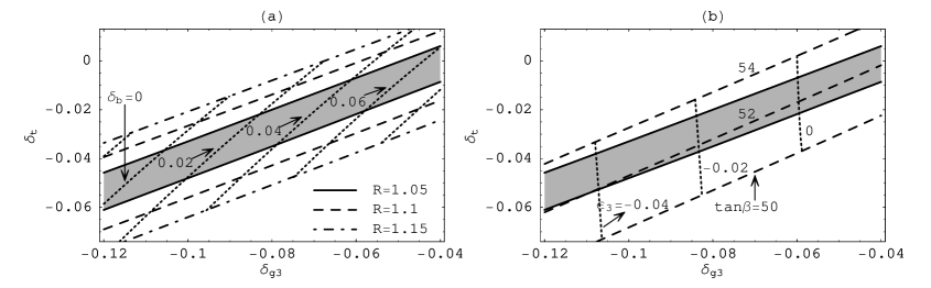
Figure 1: Parameter space satisfying the gauge-Yukawa unification. Contours of $\delta_{b}$ (dotted lines in Fig. (a)), $\tan\beta$ (dashed lines in Fig. (b)) and $\epsilon_{3}$ (dotted lines in Fig. (b)) are shown as a function of $\delta_{t}$ and $\delta_{g_{3}}$, required for Yukawa unification ($y_{t}=y_{b}=y_{\tau}$). After finding the region for the Yukawa unification, contours of a parameter $R$ (defined in text) are plotted in Fig. (a). The shaded regions represent a region where the gauge-Yukawa unification is achieved within $5\%$ level ($R\leq 1.05$). Here we have fixed $\delta_{\tau}=0.02$, $\delta_{g_{1}}=-0.006$ and $\delta_{g_{2}}=-0.02$.

First, we review gauge-Yukawa unification for the canonical case $k_{Y}=5/3$. In Fig. 1, contours of $\delta_{b}$ (dotted lines in Fig. (a)), $\tan\beta$ (dashed lines in Fig. (b)) and $\epsilon_{3}$ (dotted lines in Fig. (b)) are shown as a function of $\delta_{t}$ and $\delta_{g_{3}}$, which are required for the Yukawa unification at the GUT scale. In order to fix $\delta_{g_{1,2}}$, we assume that all SUSY mass parameters which contribute to $\delta_{g_{1,2}}$ are equal to $500$ GeV ($\delta_{g_{1}}=-0.006$ and $\delta_{g_{2}}=-0.02$). As shown in Fig. 1, $\tan\beta$ should be about $52$, and the value of $\delta_{b}$ should be a few %, which is much smaller than one naively expected in large $\tan\beta$ case. Small values of $\delta_{b}$ significantly constrains the superpartner spectrum, as discussed in Refs. [14, 11]. On the other hand, $\delta_{t}$ is in the expected range (see Ref. [15]).

After requiring Yukawa unification, we calculate a parameter $R$ defined as follows:

$$R \equiv \frac{{\rm max}(y_{G},g_{G})}{{\rm min}(y_{G},g_{G})}\,.$$ (65)

In the shaded regions of Fig. 1, gauge-Yukawa unification is realized within $5\%$ level ($R\leq 1.05$), while allowing $\epsilon_{3}$ to be a few %.

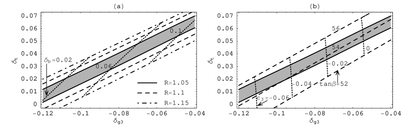
Figure 2: Same as Fig. 1, but for $k_{Y}=23/21$ with one set of $L_{x}+u_{x}$ added at $M=300$ GeV.

Next, we take $k_{Y}=23/21$ as predicted by the $SU(7)$ model, and give examples as how gauge-Yukawa unification might be realized. Gauge coupling unification can be restored by adding vector-like particles with SM quantum numbers, as in section 6. A simple example for $k_{Y}=23/21$ is adding one set of $L_{x}+u_{x}$. However, as shown in Fig. 2, Yukawa unification then requires $\delta_{t}$ shifted up 0.06 compared to Fig. 1, which is not compatible with the SUSY threshold corrections in most of the parameter space.

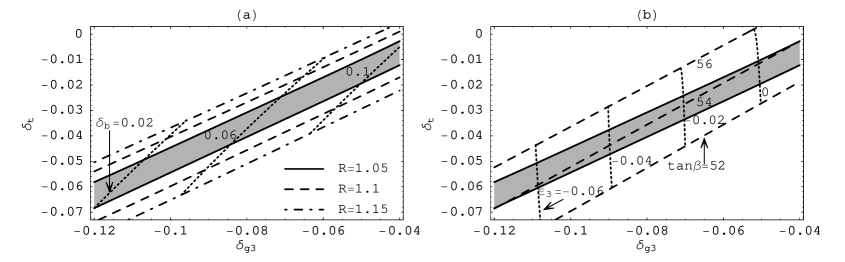
Note that $\delta_{t}$ can be modified if mixing in the top quark sector is allowed. We then have the Yukawa and mass terms

$$y_{t}Q^{\prime}H_{u}u^{\prime c}+y^{\prime}Q^{\prime}H_{u}u_{x}^{\prime c}+Mu^{\prime}_{x}u_{x}^{\prime c}~{},~{}\,$$ (66)

where the primes denote weak eigenstates. Diagonalizing the mass matrix, we obtain

$$\frac{y_{t}}{y_{t0}}=\left(\frac{2}{1+\xi^{2}+x^{2}-\sqrt{(1+\xi^{2}+x^{2})^{2}-4x^{2}}}\right)^{1/2}\,.$$ (67)

Here the notation is as follows: $y_{t0}$ is the value without mixing, $x\equiv M/m_{t}$, and $\xi\equiv y^{\prime}/y_{t}$. Experimentally, $M\lesssim 200$ GeV is excluded [16]. As an example we take $M=300$ GeV. Precision electroweak data (more precisely the bounds on the oblique parameter T) then requires the extended CKM parameter $V_{xb}\lesssim 0.4$ [17]. This constraint corresponds to $\xi\lesssim 0.5$ and a downward shift in $\delta_{t}$ of $\lesssim 0.06$.

Figure 3: Same as Fig. 1, but for $k_{Y}=23/21$ with one set of $L_{x}+d_{x}+e_{x}$ added at $M=300$ GeV. The Yukawa coupling $y_{1}$ is assumed negligible, while $y_{2}$ is taken to be $0.7$ at $M$, corresponding to $\simeq 1.5$ at the GUT scale.

A similar example is adding one set of $L_{x}+d_{x}+e_{x}$. Gauge-Yukawa unification is then obtained essentially with the same parameters as above, since the $\beta$-coefficients are identical at one loop. $\delta_{t}$ in this case can be modified even assuming no mixing, due to the new Yukawa couplings $y_{1}L_{x}H_{d}e^{c}_{x}+y_{2}L^{c}_{x}H_{u}e_{x}$. Shifting $\delta_{t}$ down appreciably requires no or a weak $y_{1}$ coupling and a strong $y_{2}$ coupling, and a numerical example is provided in Fig. 3.

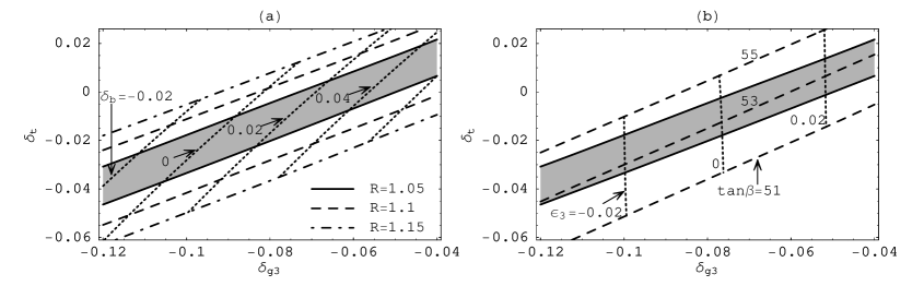
Another way to restore gauge coupling unification while preserving Yukawa unification is to add vector-like charged singlets and allowing fractional charges. As an example, we again take $k_{Y}=23/21$, and add two pairs of charged singlets with mass $m_{Z}$ and charges $\pm 1$ and $\pm 2/3$. As shown in Fig. 4, gauge-Yukawa unification is then achieved similar to the canonical case.

Figure 4: Same as Fig. 1, but for $k_{Y}=23/21$ with vector-like charged singlets (one pair with $Q=\pm 1$ and one pair with $Q=\pm 2/3$) added at $m_{Z}$.

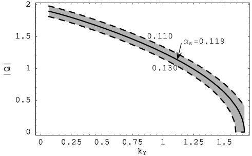
In Fig. 5, we show the charge of a vector-like charged singlet pair with mass $m_{Z}$ allowing unification, for $k_{Y}$ in the range $1/15$ to $5/3$. (Adding one pair with charges $\pm Q$ is equivalent at one-loop to adding multiple pairs with charges $\pm Q_{i}$ if $Q^{2}=\sum_{i}Q^{2}_{i}$.) Here we choose $\delta_{t,b,\tau,g_{i}}$ such that $Q=0$ for $k_{Y}=5/3$ and $\alpha^{\rm MS}_{s}(m_{Z})=0.119$. The $\pm 0.01$ uncertainty we display for $\alpha^{\rm MS}_{s}(m_{Z})$ represents both SUSY and GUT threshold corrections.

Figure 5: $|Q|$ of the vector-like charged singlet with mass $m_{Z}$ allowing unification for $k_{Y}$ in the range $1/15$ to $5/3$.

For fractionally charged singlets, there is a constraint on particle per nucleon of about $10^{-22}$ [18]. This requires the particle mass $M$ to be $\gtrsim 10^{4}T_{r}$, where $T_{r}$ is the reheating temperature [19]. Since $T_{r}$ can be as low as a few MeV, this in principle allows fractionally charged singlets as light as allowed by accelerator searches. The mass limit from accelerators is around $m_{Z}$ (for a review see Ref. [20]).

8 Higgs Mass

We end the paper with some remarks on the Higgs mass, where by the Higgs mass we refer to the mass of the light $CP$-even scalar. Assuming that $m_{Z}\ll m_{\rm SUSY}$, where $m_{\rm SUSY}$ is the characteristic supersymmetry particle mass scale, the theory below $m_{\rm SUSY}$ is the SM with threshold effects at $m_{\rm SUSY}$. The SM Higgs quartic coupling at $m_{\rm SUSY}$ is given by

$$\lambda=\frac{1}{4}(g_{Y}^{2}+g_{2}^{2})\cos^{2}2\beta=\frac{1}{4}\left(\frac{g_{2}^{2}}{\cos^{2}\theta_{W}}\right)\cos^{2}2\beta\,,$$ (68)

where $\tan\beta$ is the ratio of the two supersymmetric Higgs vacuum expectation values, and $\theta_{W}$ is the Weinberg angle. Since $\cos^{2}\theta_{W}=k_{Y}/(1+k_{Y})$ at $M_{\rm GUT}$, $\theta_{W}$ at $m_{\rm SUSY}$ depends on $k_{Y}$. The Higgs mass therefore also depends on the value of $k_{Y}$, but for SUSY broken at the TeV scale the effect is numerically insignificant, of order a few hundred MeV. The Higgs mass predictions are therefore practically the same as in canonical MSSM [21] and SUSY $SO(10)$ for the case with third-family Yukawa unification [14, 22]. The Higgs mass upper bound for $m_{t}=172.5$ GeV and $m_{\rm SUSY}=1$ TeV is $\approx 130$ GeV [21].

9 Conclusion

We have considered a class of orbifold GUTs based on 6D ${\cal N}=(1,1)$ and 7D ${\cal N}=1$ supersymmetric $SU(N)$ gauge theories, where the 4D gauge group is $SU(3)_{C}\times SU(2)_{L}\times U(1)_{Y}$ below the compactification scale. For the $SU(5)$ model the only zero mode that can be introduced in the bulk is a quark doublet, while the $SU(6)$ model allows gauge-Higgs unification. Finally, we can have gauge-Yukawa unification for the third family in $SU(7)$ or higher rank groups. Depending on the model, the $U(1)_{Y}$ normalization factor $k_{Y}$ is either uniquely determined to have a non-canonical value or lies in a continuous interval. Gauge coupling unification and gauge-Yukawa unification can be obtained for non-canonical $k_{Y}$ values by adding particles to the MSSM spectrum. As examples, we introduce a minimal set of vector-like multiplets with SM quantum numbers or fractionally charged color singlets, assuming masses in the TeV range. The existence of such particles will be tested by the upcoming LHC.

Appendix A: Six-Dimensional Orbifold Models

We consider 6D space-time which can be factorized into a product of 4D Minkowski space-time $M^{4}$ and the torus $T^{2}$ which is homeomorphic to $S^{1}\times S^{1}$. The 6D coordinates are $x^{\mu}$, ($\mu=0,1,2,3$), $x^{5}$ and $x^{6}$. The radii for the circles along the $x^{5}$ and $x^{6}$ directions are $R_{1}$ and $R_{2}$, respectively. We define the complex coordinate

$$z\equiv{1\over 2}\left(x^{5}+ix^{6}\right)~{},~{}\,$$ (69)

in which case the torus $T^{2}$ can be defined as $C^{1}$ modulo the equivalence classes:

$$z\sim z+\pi R_{1}~{},~{}z\sim z+\pi R_{2}e^{{\rm i}\theta}~{}.~{}\,$$ (70)

To define the orbifold $T^{2}/Z_{6}$, we require that $R_{1}=R_{2}\equiv R$ and $\theta=\pi/3$. Then $T^{2}/Z_{6}$ orbifold is obtained from $T^{2}$ as:

$$\Gamma_{T}:~{}~{}~{}z\sim\omega z~{},~{}\,$$ (71)

where $\omega=e^{{\rm i}\pi/3}$. There is one $Z_{6}$ fixed point: $z=0$, two $Z_{3}$ fixed points: $z=\pi Re^{{\rm i}\pi/6}/{\sqrt{3}}$ and $z=2\pi Re^{{\rm i}\pi/6}/{\sqrt{3}}$, and three $Z_{2}$ fixed points: $z=\sqrt{3}\pi Re^{{\rm i}\pi/6}/2$, $z=\pi R/2$ and $z=\pi Re^{{\rm i}\pi/3}/2$.

The ${\cal N}=(1,1)$ supersymmetry in 6D has 16 supercharges and corresponds to ${\cal N}=4$ supersymmetry in 4D, so that only the gauge multiplet can be introduced in the bulk. This multiplet can be decomposed under 4D ${\cal N}=1$ supersymmetry into a vector multiplet $V$ and three chiral multiplets $\Sigma_{1}$, $\Sigma_{2}$, and $\Sigma_{3}$ in the adjoint representation, where the fifth and sixth components of the gauge field, $A_{5}$ and $A_{6}$ are contained in the lowest component of $\Sigma_{1}$. The SM fermions can be on the 3-branes at the $Z_{6}$ fixed points. Here, we follow the conventions in Ref. [23].

For the bulk gauge group $G$, we write down the bulk action in the Wess-Zumino gauge and 4D ${\cal N}=1$ supersymmetry language [24],

$${\cal S} = \int d^{6}x\Biggl{\{}{\rm Tr}\Biggl{[}\int d^{2}\theta\left(\frac{1}{4\kappa g^{2}}{\cal W}^{\alpha}{\cal W}_{\alpha}+\frac{1}{\kappa g^{2}}\left(\Sigma_{3}\partial\Sigma_{2}-\frac{1}{\sqrt{2}}\Sigma_{1}[\Sigma_{2},\Sigma_{3}]\right)\right)+{\rm h.c.}\Biggr{]}$$ (72)

$$+\int d^{4}\theta\frac{1}{\kappa g^{2}}{\rm Tr}\Biggl{[}(\sqrt{2}\partial_{z}^{\dagger}+\Sigma_{1}^{\dagger})e^{-V}(-\sqrt{2}\partial_{z}+\Sigma_{1})e^{V}+\partial_{z}^{\dagger}e^{-V}\partial_{z}e^{V}\Biggr{]}$$

$$+\int d^{4}\theta\frac{1}{\kappa g^{2}}{\rm Tr}\Biggl{[}\Sigma_{2}^{\dagger}e^{-V}\Sigma_{2}e^{V}+{\Sigma_{3}}^{\dagger}e^{-V}\Sigma_{3}e^{V}\Biggr{]}\Biggr{\}}~{},~{}\,$$

where $\kappa$ is the normalization of the group generator, and  ${\cal W_{\alpha}}$  denotes the gauge field strength. From the above action, we obtain the transformations of the vector multiplet

$$V(x^{\mu},~{}\omega z,~{}\omega^{-1}{\bar{z}}) = R_{\Gamma_{T}}V(x^{\mu},~{}z,~{}{\bar{z}})R_{\Gamma_{T}}^{-1}~{},~{}\,$$ (73)

$$\Sigma_{1}(x^{\mu},~{}\omega z,~{}\omega^{-1}{\bar{z}}) = \omega^{-1}R_{\Gamma_{T}}\Sigma_{1}(x^{\mu},~{}z,~{}{\bar{z}})R_{\Gamma_{T}}^{-1}~{},~{}\,$$ (74)

$$\Sigma_{2}(x^{\mu},~{}\omega z,~{}\omega^{-1}{\bar{z}}) = \omega^{-1-k}R_{\Gamma_{T}}\Sigma_{2}(x^{\mu},~{}z,~{}{\bar{z}})R_{\Gamma_{T}}^{-1}~{},~{}\,$$ (75)

$$\Sigma_{3}(x^{\mu},~{}\omega z,~{}\omega^{-1}{\bar{z}}) = \omega^{2+k}R_{\Gamma_{T}}\Sigma_{3}(x^{\mu},~{}z,~{}{\bar{z}})R_{\Gamma_{T}}^{-1}~{},~{}\,$$ (76)

where $R_{\Gamma_{T}}$ is non-trivial to break the bulk gauge group $G$. To preserve 4D ${\cal N}=1$ supersymmetry, we obtain $k=0$ or $k=1$ [23].

The $Z_{6}$ transformation properties for the decomposed components of $V$, $\Sigma_{1}$, $\Sigma_{2}$, and $\Sigma_{3}$ in the $SU(7)$ models are

$$V:\left(\begin{array}[]{cccc}1&\omega^{-n_{1}}&\omega^{-n_{2}}&\omega^{-n_{3}}\\ \omega^{n_{1}}&1&\omega^{n_{1}-n_{2}}&\omega^{n_{1}-n_{3}}\\ \omega^{n_{2}}&\omega^{n_{2}-n_{1}}&1&\omega^{n_{2}-n_{3}}\\ \omega^{n_{3}}&\omega^{n_{3}-n_{1}}&\omega^{n_{3}-n_{2}}&1\end{array}\right)+1~{},~{}\,$$ (77)

$$\Sigma_{1}:\left(\begin{array}[]{cccc}\omega^{-1}&\omega^{-n_{1}-1}&\omega^{-n_{2}-1}&\omega^{-n_{3}-1}\\ \omega^{n_{1}-1}&\omega^{-1}&\omega^{n_{1}-n_{2}-1}&\omega^{n_{1}-n_{3}-1}\\ \omega^{n_{2}-1}&\omega^{n_{2}-n_{1}-1}&\omega^{-1}&\omega^{n_{2}-n_{3}-1}\\ \omega^{n_{3}-1}&\omega^{n_{3}-n_{1}-1}&\omega^{n_{3}-n_{2}-1}&\omega^{-1}\end{array}\right)+\omega^{-1}~{},~{}\,$$ (78)

$$\Sigma_{2}:\left(\begin{array}[]{cccc}\omega^{-1-k}&\omega^{-n_{1}-1-k}&\omega^{-n_{2}-1-k}&\omega^{-n_{3}-1-k}\\ \omega^{n_{1}-1-k}&\omega^{-1-k}&\omega^{n_{1}-n_{2}-1-k}&\omega^{n_{1}-n_{3}-1-k}\\ \omega^{n_{2}-1-k}&\omega^{n_{2}-n_{1}-1-k}&\omega^{-1-k}&\omega^{n_{2}-n_{3}-1-k}\\ \omega^{n_{3}-1-k}&\omega^{n_{3}-n_{1}-1-k}&\omega^{n_{3}-n_{2}-1-k}&\omega^{-1-k}\end{array}\right)+\omega^{-1-k}~{},~{}\,$$ (79)

$$\Sigma_{3}:\left(\begin{array}[]{cccc}\omega^{2+k}&\omega^{-n_{1}+2+k}&\omega^{-n_{2}+2+k}&\omega^{-n_{3}+2+k}\\ \omega^{n_{1}+2+k}&\omega^{2+k}&\omega^{n_{1}-n_{2}+2+k}&\omega^{n_{1}-n_{3}+2+k}\\ \omega^{n_{2}+2+k}&\omega^{n_{2}-n_{1}+2+k}&\omega^{2+k}&\omega^{n_{2}-n_{3}+2+k}\\ \omega^{n_{3}+2+k}&\omega^{n_{3}-n_{1}+2+k}&\omega^{n_{3}-n_{2}+2+k}&\omega^{2+k}\end{array}\right)+\omega^{2+k}~{},~{}\,$$ (80)

where the zero modes transform as $1$. Note that $n_{1}\not=n_{2}\not=n_{3}\not=0$ and from Eqs. (77)–(80), we obtain that for the zero modes, the 6D ${\cal N}=(1,1)$ supersymmetric $SU(7)$ gauge symmetry is broken down to 4D ${\cal N}=1$ supersymmetric $SU(3)_{C}\times SU(2)_{L}\times U(1)_{Y}\times U(1)_{\beta}\times U(1)_{\gamma}$ gauge symmetry.

Appendix B: Seven-Dimensional Orbifold Models

We consider a 7D space-time $M^{4}\times T^{2}/Z_{6}\times S^{1}/Z_{2}$ with coordinates $x^{\mu}$, ($\mu=0,1,2,3$), $x^{5}$, $x^{6}$ and $x^{7}$. The torus $T^{2}$ is homeomorphic to $S^{1}\times S^{1}$ and the radii of the circles along the $x^{5}$, $x^{6}$ and $x^{7}$ directions are $R_{1}$, $R_{2}$, and $R^{\prime}$, respectively. We introduce a complex coordinate $z$ for $T^{2}$ and a real coordinate $y$ for $S^{1}$,

$$z\equiv{1\over 2}\left(x^{5}+ix^{6}\right),~{}~{}~{}~{}~{}~{}~{}~{}~{}~{}y\equiv x^{7}.$$ (81)

The orbifold $T^{2}/Z_{6}$ has been defined in Appendix A, while the orbifold $S^{1}/Z_{2}$ is obtained from $S^{1}$ by moduloing the equivalent class

$$\Gamma_{S}:~{}~{}~{}y\sim-y~{}.~{}\,$$ (82)

There are two fixed points: $y=0$ and $y=\pi R^{\prime}$.

The 7D ${\cal N}=1$ supersymmetry has 16 supercharges corresponding to ${\cal N}=4$ supersymmetry in 4D, and only the gauge multiplet can be introduced in the bulk. This multiplet can be decomposed under 4D ${\cal N}=1$ supersymmetry into a gauge vector multiplet $V$ and three chiral multiplets $\Sigma_{1}$, $\Sigma_{2}$, and $\Sigma_{3}$, all in the adjoint representation, where the fifth and sixth components of the gauge field, $A_{5}$ and $A_{6}$, are contained in the lowest component of $\Sigma_{1}$, and the seventh component of the gauge field $A_{7}$ is contained in the lowest component of $\Sigma_{2}$.

We express the bulk action in the Wess–Zumino gauge and 4D ${\cal N}=1$ supersymmetry notation [24]

$${\cal S} = \int d^{7}x\Biggl{\{}{\rm Tr}\Biggl{[}\int d^{2}\theta\left(\frac{1}{4\kappa g^{2}}{\cal W}^{\alpha}{\cal W}_{\alpha}+\frac{1}{\kappa g^{2}}\left(\Sigma_{3}\partial_{z}\Sigma_{2}+\Sigma_{1}\partial_{y}\Sigma_{3}-\frac{1}{\sqrt{2}}\Sigma_{1}[\Sigma_{2},\Sigma_{3}]\right)\right)$$ (83)

$$+h.c.\Biggr{]}+\int d^{4}\theta\frac{1}{\kappa g^{2}}{\rm Tr}\Biggl{[}(\sqrt{2}\partial_{z}^{\dagger}+\Sigma_{1}^{\dagger})e^{-V}(-\sqrt{2}\partial_{z}+\Sigma_{1})e^{V}+\partial_{z}^{\dagger}e^{-V}\partial_{z}e^{V}$$

$$+(\sqrt{2}\partial_{y}+\Sigma_{2}^{\dagger})e^{-V}(-\sqrt{2}\partial_{y}+\Sigma_{2})e^{V}+\partial_{y}e^{-V}\partial_{y}e^{V}+{\Sigma_{3}}^{\dagger}e^{-V}\Sigma_{3}e^{V}\Biggr{]}\Biggr{\}}.~{}\,$$

From the above action, we obtain the transformations of the vector multiplet:

$$V(x^{\mu},~{}\omega z,~{}\omega^{-1}{\bar{z}},~{}y) = R_{\Gamma_{T}}V(x^{\mu},~{}z,~{}{\bar{z}},~{}y)R_{\Gamma_{T}}^{-1}~{},~{}\,$$ (84)

$$\Sigma_{1}(x^{\mu},~{}\omega z,~{}\omega^{-1}{\bar{z}},~{}y) = \omega^{-1}R_{\Gamma_{T}}\Sigma_{1}(x^{\mu},~{}z,~{}{\bar{z}},~{}y)R_{\Gamma_{T}}^{-1}~{},~{}\,$$ (85)

$$\Sigma_{2}(x^{\mu},~{}\omega z,~{}\omega^{-1}{\bar{z}},~{}y) = R_{\Gamma_{T}}\Sigma_{2}(x^{\mu},~{}z,~{}{\bar{z}},~{}y)R_{\Gamma_{T}}^{-1}~{},~{}\,$$ (86)

$$\Sigma_{3}(x^{\mu},~{}\omega z,~{}\omega^{-1}{\bar{z}},~{}y) = \omega R_{\Gamma_{T}}\Sigma_{3}(x^{\mu},~{}z,~{}{\bar{z}},~{}y)R_{\Gamma_{T}}^{-1}~{},~{}\,$$ (87)

$$V(x^{\mu},~{}z,~{}{\bar{z}},~{}-y) = R_{\Gamma_{S}}V(x^{\mu},~{}z,~{}{\bar{z}},~{}y)R_{\Gamma_{S}}^{-1}~{},~{}\,$$ (88)

$$\Sigma_{1}(x^{\mu},~{}z,~{}{\bar{z}},~{}-y) = R_{\Gamma_{S}}\Sigma_{1}(x^{\mu},~{}z,~{}{\bar{z}},~{}y)R_{\Gamma_{S}}^{-1}~{},~{}\,$$ (89)

$$\Sigma_{2}(x^{\mu},~{}z,~{}{\bar{z}},~{}-y) = -R_{\Gamma_{S}}\Sigma_{2}(x^{\mu},~{}z,~{}{\bar{z}},~{}y)R_{\Gamma_{S}}^{-1}~{},~{}\,$$ (90)

$$\Sigma_{3}(x^{\mu},~{}z,~{}{\bar{z}},~{}-y) = -R_{\Gamma_{S}}\Sigma_{3}(x^{\mu},~{}z,~{}{\bar{z}},~{}y)R_{\Gamma_{S}}^{-1}~{},~{}\,$$ (91)

where we introduce non-trivial transformations $R_{\Gamma_{T}}$ and $R_{\Gamma_{S}}$ to break the bulk gauge group $G$.

The $Z_{6}\times Z_{2}$ transformation properties for the decomposed components of $V$, $\Sigma_{1}$, $\Sigma_{2}$, and $\Sigma_{3}$ in the $SU(8)$ model are given by

$$V:\left(\begin{array}[]{ccccc}(1,+)&(\omega^{-n_{1}},+)&(\omega^{-n_{1}},-)&(1,-)&(\omega^{-n_{2}},+)\\ (\omega^{n_{1}},+)&(1,+)&(1,-)&(\omega^{n_{1}},-)&(\omega^{n_{1}-n_{2}},+)\\ (\omega^{n_{1}},-)&(1,-)&(1,+)&(\omega^{n_{1}},+)&(\omega^{n_{1}-n_{2}},-)\\ (1,-)&(\omega^{-n_{1}},-)&(\omega^{-n_{1}},+)&(1,+)&(\omega^{-n_{2}},-)\\ (\omega^{n_{2}},+)&(\omega^{n_{2}-n_{1}},+)&(\omega^{n_{2}-n_{1}},-)&(\omega^{n_{2}},-)&(1,+)\end{array}\right)+(1,+)~{},~{}\,$$ (92)

$$\Sigma_{1}:\left(\begin{array}[]{ccccc}(\omega^{-1},+)&(\omega^{-n_{1}-1},+)&(\omega^{-n_{1}-1},-)&(\omega^{-1},-)&(\omega^{-n_{2}-1},+)\\ (\omega^{n_{1}-1},+)&(\omega^{-1},+)&(\omega^{-1},-)&(\omega^{n_{1}-1},-)&(\omega^{n_{1}-n_{2}-1},+)\\ (\omega^{n_{1}-1},-)&(\omega^{-1},-)&(\omega^{-1},+)&(\omega^{n_{1}-1},+)&(\omega^{n_{1}-n_{2}-1},-)\\ (\omega^{-1},-)&(\omega^{-n_{1}-1},-)&(\omega^{-n_{1}-1},+)&(\omega^{-1},+)&(\omega^{-n_{2}-1},-)\\ (\omega^{n_{2}-1},+)&(\omega^{n_{2}-n_{1}-1},+)&(\omega^{n_{2}-n_{1}-1},-)&(\omega^{n_{2}-1},-)&(\omega^{-1},+)\end{array}\right)+(\omega^{-1},+)~{},~{}\,$$ (93)

$$\Sigma_{2}:\left(\begin{array}[]{ccccc}(1,-)&(\omega^{-n_{1}},-)&(\omega^{-n_{1}},+)&(1,+)&(\omega^{-n_{2}},-)\\ (\omega^{n_{1}},-)&(1,-)&(1,+)&(\omega^{n_{1}},+)&(\omega^{n_{1}-n_{2}},-)\\ (\omega^{n_{1}},+)&(1,+)&(1,-)&(\omega^{n_{1}},-)&(\omega^{n_{1}-n_{2}},+)\\ (1,+)&(\omega^{-n_{1}},+)&(\omega^{-n_{1}},-)&(1,-)&(\omega^{-n_{2}},+)\\ (\omega^{n_{2}},-)&(\omega^{n_{2}-n_{1}},-)&(\omega^{n_{2}-n_{1}},+)&(\omega^{n_{2}},+)&(1,-)\end{array}\right)+(1,-)~{},~{}\,$$ (94)

$$\Sigma_{3}:\left(\begin{array}[]{ccccc}(\omega,-)&(\omega^{-n_{1}+1},-)&(\omega^{-n_{1}+1},+)&(\omega,+)&(\omega^{-n_{2}+1},-)\\ (\omega^{n_{1}+1},-)&(\omega,-)&(\omega,+)&(\omega^{n_{1}+1},+)&(\omega^{n_{1}-n_{2}+1},-)\\ (\omega^{n_{1}+1},+)&(\omega,+)&(\omega,-)&(\omega^{n_{1}+1},-)&(\omega^{n_{1}-n_{2}+1},+)\\ (\omega,+)&(\omega^{-n_{1}+1},+)&(\omega^{-n_{1}+1},-)&(\omega,-)&(\omega^{-n_{2}+1},+)\\ (\omega^{n_{2}+1},-)&(\omega^{n_{2}-n_{1}+1},-)&(\omega^{n_{2}-n_{1}+1},+)&(\omega^{n_{2}+1},+)&(\omega,-)\end{array}\right)+(\omega,-)~{},~{}\,$$ (95)

From Eqs. (92)–(95), we obtain that the 7D ${\cal N}=1$ supersymmetric $SU(8)$ gauge symmetry is broken down to 4D ${\cal N}=1$ supersymmetric $SU(3)_{C}\times SU(2)_{L}\times U(1)_{Y}\times U(1)_{\alpha}\times U(1)_{\beta}\times U(1)_{\gamma}$ gauge symmetry [2].

References

[1] See, for example,
Y. Kawamura,
Prog. Theor. Phys. 103, 613 (2000); 105, 999 (2001); G.
Altarelli and F. Feruglio, Phys. Lett. B 511, 257 (2001);
A. B. Kobakhidze, Phys. Lett. B 514, 131 (2001);
L. Hall and Y. Nomura, Phys. Rev. D 64, 055003 (2001); A.
Hebecker and J. March-Russell, Nucl. Phys. B 613, 3 (2001).
[2]
T. Li, Phys. Lett. B 520, 377 (2001); Nucl. Phys. B 619, 75 (2001);
Nucl. Phys. B 633, 83 (2002).
[3]
V. Barger, J. Jiang, P. Langacker and T. Li,
Phys. Lett. B 624, 233 (2005);
Nucl. Phys. B 726, 149 (2005).
[4]
I. Gogoladze, T. Li and Q. Shafi,
Phys. Rev. D 73, 066008 (2006).
[5]
I. Gogoladze, T. Li, V. N. Senoguz and Q. Shafi,
arXiv:hep-ph/0604217.
[6]
See, for example,
I. Antoniadis, K. Benakli and M. Quiros,
New J. Phys. 3, 20 (2001);
G. R. Dvali, S. Randjbar-Daemi and R. Tabbash,
Phys. Rev. D 65, 064021 (2002);
G. Burdman and Y. Nomura,
Nucl. Phys. B 656 (2003) 3;
N. Haba and Y. Shimizu,
Phys. Rev. D 67 (2003) 095001;
K. w. Choi, N. y. Haba, K. S. Jeong, K. i. Okumura, Y. Shimizu and
M. Yamaguchi,
JHEP 0402, 037 (2004);
Q. Shafi and Z. Tavartkiladze,
Phys. Rev. D 66, 115002 (2002),
I. Gogoladze, Y. Mimura, S. Nandi,
Phys. Lett. B 560 (2003) 204;
C. A. Scrucca, M. Serone, L. Silvestrini and A. Wulzer,
JHEP 0402, 049 (2004);
G. Panico, M. Serone and A. Wulzer,
arXiv:hep-ph/0510373.
A. Aranda and J. L. Diaz-Cruz,
arXiv:hep-ph/0510138.
N. Haba, S. Matsumoto, N. Okada and T. Yamashita,
arXiv:hep-ph/0511046.
Y. Hosotani, S. Noda, Y. Sakamura and S. Shimasaki,
arXiv:hep-ph/0601241.
[7]
I. Gogoladze, Y. Mimura and S. Nandi,
Phys. Lett. B 562, 307 (2003); Phys. Rev. Lett. 91, 141801
(2003); Phys. Rev. D 69, 075006 (2004); I. Gogoladze, Y. Mimura, S. Nandi and K. Tobe,
Phys. Lett. B 575, 66 (2003);
I. Gogoladze, T. Li, Y. Mimura and S. Nandi,
Phys. Lett. B 622, 320 (2005); Phys. Rev. D 72, 055006
(2005).
[8]
C. D. Froggatt and H. B. Nielsen, Nucl. Phys. B 147, 277 (1979).
[9]
G. F. Giudice and A. Masiero,
Phys. Lett. B 206, 480 (1988).
[10]
I. Gogoladze,
Y. Mimura,
S. Nandi, and
K. Tobe,
Phys. Lett. B 575,
66 (2003).
[11]
K. Tobe and
J. D. Wells,
Nucl. Phys. B 663,
123 (2003).
[12]
[Tevatron Electroweak Working Group],
arXiv:hep-ex/0603039.
[13]
S. Eidelman et al.
(Particle Data Group), Phys.
Lett. B 592, 1
(2004).
[14]
T. Blazek,
R. Dermisek, and
S. Raby,
Phys. Rev. Lett. 88,
111804 (2002);
Phys. Rev. D 65,
115004 (2002).
[15]
D. M. Pierce, J. A. Bagger, K. T. Matchev and R. j. Zhang,
Nucl. Phys. B 491, 3 (1997).
[16]
D. Acosta et al. [CDF Collaboration],
Phys. Rev. Lett. 90, 131801 (2003).
[17]
J. A. Aguilar-Saavedra,
Phys. Rev. D 67, 035003 (2003)
[Erratum-ibid. D 69, 099901 (2004)].
[18]
I. T. Lee et al.,
Phys. Rev. D 66,
012002 (2002).
[19]
A. Kudo and
Phys. Lett. B 516,
151 (2001).
[20]
M. L. Perl,
E. R. Lee, and
D. Loomba,
Mod. Phys. Lett. A 19,
2595 (2004).
[21]
M. Carena, J. R. Espinosa, M. Quiros and C. E. M. Wagner,
Phys. Lett. B 355, 209 (1995);
M. Carena, M. Quiros and C. E. M. Wagner,
Nucl. Phys. B 461, 407 (1996);
H. E. Haber, R. Hempfling and A. H. Hoang,
Z. Phys. C 75, 539 (1997);
G. Degrassi, S. Heinemeyer, W. Hollik, P. Slavich and G. Weiglein,
Eur. Phys. J. C 28, 133 (2003).
[22]
Q. Shafi and B. Ananthanarayan, in Proceedings of the Summer School in high energy physics and cosmology,
Trieste, Italy, 1991, edited by E. Gava et al. (World Scientific, 1992), p. 233;
B. Ananthanarayan, Q. Shafi and X. M. Wang,
Phys. Rev. D 50, 5980 (1994);
D. Auto, H. Baer, C. Balazs, A. Belyaev, J. Ferrandis and X. Tata,
JHEP 0306, 023 (2003).
[23]
T. Li,
JHEP 0403, 040 (2004).
[24]
N. Marcus, A. Sagnotti and W. Siegel, Nucl. Phys. B 224, 159
(1983); N. Arkani-Hamed, T. Gregoire and J. Wacker,
JHEP 0203, 055 (2002).