Recursive Construction of Higgs $+$ Multiparton Loop Amplitudes:
The Last of the $\phi$-nite Loop Amplitudes

Abstract

We consider a scalar field, such as the Higgs boson $H$, coupled to gluons via the effective operator $H\mathop{\rm tr}\nolimits G_{\mu\nu}G^{\mu\nu}$ induced by a heavy-quark loop. We treat $H$ as the real part of a complex field $\phi$ which couples to the self-dual part of the gluon field-strength, via the operator $\phi\mathop{\rm tr}\nolimits G_{{\scriptscriptstyle SD}\,\mu\nu}G_{\scriptscriptstyle SD}^{\mu\nu}$, whereas the conjugate field $\phi^{\dagger}$ couples to the anti-self-dual part. There are three infinite sequences of amplitudes coupling $\phi$ to quarks and gluons that vanish at tree level, and hence are finite at one loop, in the QCD coupling. Using on-shell recursion relations, we find compact expressions for these three sequences of amplitudes and discuss their analytic properties.

I Introduction

In the next year, the Large Hadron Collider (LHC) will begin operation at CERN, ushering in a new regime of directly probing physics at the shortest distance scales. The LHC will search for physics beyond the Standard Model, as well as for the Higgs boson. The Higgs mechanism, which describes the breaking of electroweak symmetry in the Standard Model and its supersymmetric extensions, is simultaneously the keystone of the Standard Model (SM) and its least-well-tested ingredient.

The dominant process for Higgs-boson production, over the entire range of Higgs masses relevant for the LHC, is the gluon fusion process, $gg\to H$, which is mediated by a heavy-quark loop Georgi1977gs . The leading contribution comes from the top quark. The contributions from other quarks are suppressed by at least a factor of ${\cal O}(m_{b}^{2}/m_{t}^{2})$, where $m_{t},m_{b}$ are the mass of the top and of the bottom quark, respectively. Because the Higgs boson is produced via a heavy-quark loop, the calculation of the production rate is quite involved, even at leading order in $\alpha_{s}$. The inclusive production rate for $gg\to H+X$ has been computed at next-to-leading order (NLO) in $\alpha_{s}$ NLOHiggs , including the full quark-mass dependence NLOHiggsExact , which required an evaluation at two-loop accuracy. The NLO QCD corrections increase the production rate by close to 100%. However, in the large-$m_{t}$ limit, namely if the Higgs mass $m_{H}$ is smaller than the threshold for the creation of a top-quark pair, $m_{H}<2\,m_{t}$, the coupling of the Higgs to the gluons via a top-quark loop can be replaced by an effective coupling NLOHiggs ; HggOperator ; HggOperator2 . This approximation simplifies calculations tremendously, because it effectively reduces the number of loops in a given diagram by one.

It has been shown that one can approximate the full NLO QCD corrections quite accurately by computing the NLO QCD correction factor, $K^{\rm NLO}\equiv\sigma^{\rm NLO}/\sigma^{\rm LO}$, in the large-$m_{t}$ limit, and multiplying it by the exact leading-order calculation. This approximation is good to within 10% in the entire Higgs-mass range at the LHC, i.e. up to 1 TeV Kramer1996iq . The reason it works so well is that the QCD corrections to $gg\to H$ are dominated by soft-gluon effects, which do not resolve the top-quark loop that mediates the coupling of the Higgs boson to the gluons. The next-to-next-to-leading order (NNLO) corrections to the production rate for $gg\to H$ have been evaluated in the large-$m_{t}$ limit NNLOHiggs and display a modest increase, less than 20%, with respect to the NLO evaluation. The dominant part of the NNLO corrections comes from virtual, soft, and collinear gluon radiation Catani2001ic , in agreement with the observations at NLO. In addition, the threshold resummation of soft-gluon effects Kramer1996iq ; Catani2003zt enhances the NNLO result by less than 10%, showing that the calculation has largely stabilized by NNLO. The soft and collinear terms have recently been evaluated to one more order (N³LO) MochVogt , with partial results to N⁴LO Ravindran , which further reduces the uncertainty on the inclusive production cross section.

Backgrounds from SM physics are usually quite large and hamper the Higgs-boson search. A process that promises to have a more amenable background is Higgs production in association with a high transverse-energy ($E_{T}$) jet, $pp\to H\,+$ jet. In addition, this process offers the advantage of being more flexible in the choice of acceptance cuts to curb the background. The $pp\to H\,+$ jet process is known exactly at leading order Ellis1988xu , while the NLO calculation deFlorian1999zd has been performed in the large-$m_{t}$ limit. For Higgs $+$ jet production, the large-$m_{t}$ limit is valid as long as $m_{H}<2\,m_{t}$ and the transverse energy $E_{T}$ is smaller than the top-quark mass, $E_{T}<m_{t}$ Baur1989cm . As long as these conditions hold, the jet-Higgs invariant mass can be taken larger than $m_{t}$ H2j . At $m_{H}=120$ GeV, the NLO corrections to the $pp\to H\,+$ jet process increase the leading-order prediction by about 60%, and are thus of the same order as the NLO corrections to fully inclusive $pp\to H$ production considered above. At present, the NNLO corrections to $pp\to H\,+$ jet are not known.

An even more interesting process is Higgs production in association with two jets. In fact, a key component of the program to measure the Higgs-boson couplings at the LHC is the vector-boson fusion (VBF) process, $qq\to qqH$ via $t$-channel $W$ or $Z$ exchange. This process is characterized by two forward quark jets Zeppenfeld2000td . The NLO corrections to Higgs production via VBF fusion in association with two jets are known to be small NLOWBFFOZ . Thus, small theoretical uncertainties are predicted for this production process. The production of $H\,+2$ jets via gluon fusion is a part of the inclusive Higgs production signal. However, it constitutes a background when trying to isolate the $HWW$ and $HZZ$ couplings responsible for the VBF process. A precise description of this background is needed in order to separate the two major sources of $H\,+$ 2 jets events: one needs to find characteristic distributions that distinguish VBF from gluon fusion.

The production of $H+2$ jets via gluon fusion is known at leading order in the large-$m_{t}$ limit DawsonKauffman and exactly H2j2 . As in the case of $H+1$ jet production, the large-$m_{t}$ limit is valid as long as $m_{H}<2\,m_{t}$ and the jet transverse energies are smaller than the top-quark mass, $E_{T,1},E_{T,2}<m_{t}$, even if the dijet mass, as well as either of the jet-Higgs masses, is larger than the top-quark mass H2j . At present, the NLO calculation for the production of $H\,+$ 2 jets via gluon fusion has not yet been completed, not even in the large-$m_{t}$ limit, although the necessary amplitudes, namely the one-loop amplitudes for a Higgs boson plus four partons EGZHiggs and the tree amplitudes for a Higgs boson plus five partons DFM ; DGK ; BGK , have been computed. Considering the aforementioned results for the NLO corrections to fully inclusive Higgs production and to Higgs production in association with one jet, and the fact that the largest NLO corrections are usually found in gluon-initiated processes, there is no reason to expect that the NLO corrections to $H+\,2$ jets production via gluon fusion are small. Thus, such a NLO calculation is highly desirable.

Another distinguishing feature of VBF is that to leading order, and with a good approximation also to NLO, no color is exchanged in the $t$ channel Dokshitzer1987nc . The different gluon-radiation pattern expected for Higgs production via VBF versus its major backgrounds, namely $t\bar{t}$ production and QCD $WW+2$ jet production, is at the core of the central-jet veto proposal, both for heavy Barger1994zq and light Kauer2000hi Higgs searches. A veto of any additional jet activity in the central-rapidity region is expected to suppress the backgrounds more than the signal, because the QCD backgrounds are characterized by quark or gluon exchange in the $t$ channel. The exchange of colored partons should lead to more central gluon radiation. In the case of Higgs production via gluon fusion, with two jets separated by a large rapidity interval, the scattering process is dominated by gluon exchange in the $t$ channel. Thus, as for the QCD backgrounds, the bremsstrahlung radiation is expected to occur everywhere in rapidity, and Higgs production via gluon fusion can be likewise checked by requiring a central-jet veto. For hard radiation, the effectiveness of such a veto may be analyzed through $H+\,3$ jets production, which for gluon fusion is known in the large-$m_{t}$ limit at leading order DFM . An analogous study that also includes soft radiation has just been completed, by interfacing matrix-element calculations of $H+\,2$ and 3 jets production with parton-shower effects DelDuca2006hk .

The discussion above motivates us to look for methods to compute Higgs production in association with many jets at least to NLO or higher accuracy. Tree amplitudes for a Higgs boson produced via gluon fusion together with many partons have been computed analytically in the large-$m_{t}$ limit DGK ; BGK and are available numerically through the matrix-element Monte Carlo generators ALPGEN ALPGEN and MADEVENT MADGRAPH . However, at one loop only the QCD amplitudes for a Higgs boson plus up to four partons are known EGZHiggs . The three-parton helicity amplitudes were computed analytically in the large-$m_{t}$ limit Schmidt . The four-parton results are semi-numerical, except for two cases: (1) analytic results have been presented for the case of two quark-antiquark pairs EGZHiggs , and (2) the case of four gluons all with the same helicity is now known analytically as well BadgerGloverH4g .

Recently a lot of progress has been made in the computation of tree-level gauge-theory amplitudes DGK ; BGK ; CSW ; Currents ; RSVNewTree ; BCFRecursion ; BCFW ; LuoWen ; BFRSV ; BadgerMassive ; BadgerVector , following Witten’s proposal WittenTopologicalString of a weak-weak coupling duality between ${\cal N}=4$ supersymmetric gauge theory and the topological open-string $B$ model in twistor space (for a review, see ref. CSReview ). Recursion relations for computing tree amplitudes have been written BCFRecursion ; BCFW which employ only on-shell amplitudes at complex values of the external momenta. Likewise, progress has been made in the computation of one-loop amplitudes BST ; BCF7 ; NeqFourSevenPoint ; BCFII ; NeqFourNMHV ; OtherGaugeCalcs ; BBCF ; BFM ; OnShellRecursionI ; LastFinite ; Bootstrapping ; FordeKosower ; BBDFK1 ; BBDFK2 , particularly those with many external legs, for which there are many different kinematic variables. If careful attention is not paid to the analytic structure, very large analytic expressions may result. One approach to this problem is to compute the loop amplitudes numerically or semi-numerically NumericalLoops ; EGZHiggs ; Zanderighi06 . Another approach is to exploit the analytic properties of the amplitudes in order to facilitate their computation. The two main analytic properties of loop amplitudes are branch cuts and factorization poles.

In pure QCD with massless quarks, there are special helicity configurations for which the tree amplitudes vanish, and the corresponding one-loop amplitudes are finite. Such helicity amplitudes are of no immediate use in phenomenology, because they contribute first at NNLO. However, they have interesting analytic properties. The specific helicity amplitudes in this category are the pure-glue one-loop amplitudes for which all the gluons have the same helicity, or else all but one do, namely, ${\cal A}_{n}^{{(1)}}(1^{\pm},2^{+},3^{+},\ldots,n^{+})$; and in addition the amplitudes with one pair of massless external quarks and $(n-2)$ positive-helicity gluons, ${\cal A}_{n}^{{(1)}}(1_{\bar{q}}^{-},2_{q}^{+},3^{+},\ldots,n^{+})$. These amplitudes contain no branch cuts; they are purely rational functions of the kinematic variables AllPlus ; Mahlon . Compact forms for the amplitudes have been found by constructing on-shell recursion relations, along the lines of the tree-level relations BCFRecursion ; BCFW , and then solving them in closed form OnShellRecursionI ; LastFinite .

All the other one-loop helicity amplitudes in QCD contain branch cuts. The terms with branch cuts can be determined from unitarity in four dimensions; then recursion relations can be established for the remaining rational terms Bootstrapping ; BBDFK1 . This approach offers an efficient way in principle of building up a generic $n$-point one-loop amplitude from one-loop amplitudes with a smaller number of points. It has been applied in practice to determine the rational parts of the $n$-gluon amplitudes with two negative-helicity gluons in arbitrary locations in the color ordering FordeKosower ; BBDFK2 , and also for cases with three or four color-adjacent negative-helicity gluons BBDFK1 . (For $n=6$, the rational terms for three color-nonadjacent negative-helicity gluons, as well as two negative-helicity ones, have been worked out XYZ6pt using Feynman-diagrammatic methods XYZmethod .)

A closely-related framework can be constructed for amplitudes for a scalar field, such as the Higgs boson $H$, interacting with an arbitrary number of quarks and gluons. In the large-$m_{t}$ limit, the Higgs field couples to gluons via the effective operator $H\mathop{\rm tr}\nolimits G_{\mu\nu}G^{\mu\nu}$ induced by the heavy-quark loop. To make the situation parallel to the pure-QCD case, we follow refs. DGK ; BGK and treat $H$ as the real part of a complex field $\phi$. Here $\phi$ couples to the self-dual part of the gluon field strength via the operator $\phi\mathop{\rm tr}\nolimits G_{{\scriptscriptstyle SD}\,\mu\nu}G_{\scriptscriptstyle SD}^{\mu\nu}$, whereas the conjugate field $\phi^{\dagger}$ couples to the anti-self-dual part. Then, exactly as in the case of pure QCD (i.e. when $\phi$ is absent), the amplitudes ${\cal A}_{n}(\phi,1^{\pm},2^{+},3^{+},\ldots,n^{+})$ and ${\cal A}_{n}(\phi,1_{\bar{q}}^{-},2_{q}^{+},3^{+},\ldots,n^{+})$ vanish at tree level, and are free of branch cuts at one loop. (They are also free of infrared and ultraviolet divergences.) Thus the one-loop amplitudes, ${\cal A}_{n}^{{(1)}}(\phi,1^{\pm},2^{+},3^{+},\ldots,n^{+})$ and ${\cal A}_{n}^{{(1)}}(\phi,1_{\bar{q}}^{-},2_{q}^{+},3^{+},\ldots,n^{+})$, can be written as rational functions of the kinematic variables. The $\phi^{\dagger}$ amplitudes are obtained from the $\phi$ amplitudes by parity, which also reverses all parton helicities. Amplitudes containing a scalar Higgs field $H$ are given by the sum of the $\phi$ and $\phi^{\dagger}$ amplitudes; whereas amplitudes containing a pseudoscalar field $A$ instead are found from the difference of the two amplitudes. In these sums and differences, the finite $\phi$ amplitudes have to be combined with the image under parity of divergent $\phi$ amplitudes with mostly negative gluon helicities.

The aim of this paper is to construct and solve on-shell recursion relations for the finite one-loop amplitudes with a single scalar field $\phi$. To assemble complete analytic helicity amplitudes for $H$ or $A$ fields, other, divergent helicity configurations are also required. These are the $\phi^{\dagger}$ amplitudes with the same helicity configurations as those computed here, or equivalently, the $\phi$ amplitudes with all parton helicities reversed. The full set of helicity amplitudes for $H$ or $A$ fields requires as well $\phi$ amplitudes with two or more negative parton helicities and two or more positive helicities. We leave such computations to future work — except that we shall quote the recent results of ref. BadgerGloverH4g for four identical-helicity gluons. We stress, however, that the amplitudes we compute represent one piece in the $\phi$-$\phi^{\dagger}$ decomposition of $H$ or $A$ amplitudes for which the corresponding tree amplitudes are nonvanishing. Hence they contribute to NLO Higgs cross sections. (This is in contrast to the finite amplitudes in pure QCD, without a $\phi$ field, which first contribute at NNLO.) A second reason why the finite $\phi$ amplitudes are useful is that in the recursive approach we pursue, amplitudes with few negative helicities are needed to supply factorization information for amplitudes with more legs and more negative helicities.

The construction of on-shell recursion relations relies on information about the factorization properties of amplitudes, as momentum invariants built from two or more external momenta become null. In the “collinear” case of two external momenta, this behavior, involving complex momenta, is quite subtle at the loop level. Loop amplitudes can contain double poles in collinear invariants OnShellRecursionI , and “unreal” poles for which the collinear limit in real momenta is not singular, yet nonetheless a single pole arises for complex momenta LastFinite . In our recursive approach to the finite quark-gluon amplitudes, ${\cal A}_{n}^{{(1)}}(\phi,1_{\bar{q}}^{-},2_{q}^{+},3^{+},\ldots,n^{+})$, we encounter both these types of poles. A knowledge of the residues at these poles is essential for constructing correct recursion relations. It might be possible to rigorously analyze such contributions using “space-cone” gauge techniques CSandVY . In this paper we adopt a much more pragmatic approach; indeed, we argue that the unreal poles take precisely the same form as in the pure-QCD case LastFinite , for which several types of consistency checks were available.

Using this approach, we present recursion relations for the finite $\phi$-quark amplitudes with an arbitrary number of external gluons. We find compact solutions to the relations, valid for all $n$. To confirm these relations we perform nontrivial consistency checks of the factorization properties of the solutions. One of the factorizations, as the momenta of the quark and anti-quark become collinear, is onto the one-loop $\phi$-plus-$n$-gluon amplitudes with a single negative gluon helicity and the rest positive, and determines this sequence of amplitudes.

The $\phi$-amplitudes with two or more negative helicities can be obtained by extensions of the methods of refs. Neq4Oneloop ; UnitarityMachinery ; BCFII ; Bootstrapping ; BBDFK1 ; BBDFK2 . Unitarity (or the related loop-level application of maximally-helicity-violating (MHV) rules BST ) can be used to determine the cut-containing functions from known tree-level amplitudes Neq4Oneloop ; UnitarityMachinery ; BCFII . The cut-containing parts of Higgs amplitudes with an arbitrary number of identical-helicity gluons have been found in this way BadgerGloverH4g . The remaining rational functions can then be computed via a factorization bootstrap approach, in the form of on-shell recursion relations analogous to the approach of ref. Bootstrapping ; BBDFK1 ; BBDFK2 in the pure-QCD case. In this publication, however, we mainly concentrate on the amplitudes with one or no negative helicities, which do not contain any cuts.

The paper is organized as follows: After introducing some convenient notation in section II, we review the on-shell recursion relations in section III and the previously-known one-loop finite amplitudes in pure QCD in section IV.1. In section IV.2 we summarize known results for amplitudes with a $\phi$ field and present a recursion relation for the MHV tree-level $\phi$-plus-$n$-gluon amplitudes, ${\cal A}_{n}^{{(0)}}(\phi,1^{+},\ldots,i^{-},\ldots,j^{-},\ldots,n^{+})$. In section V we discuss some interesting features of the soft-Higgs limit of the $\phi$ amplitudes, as the momentum of $\phi$ vanishes. In the tree-level case, the soft-Higgs limit always produces a fixed, helicity-dependent multiple of the corresponding QCD amplitude. At one loop, however, this is not true in general, although it is true for the finite $\phi$ amplitudes DGK .

In section VI we present and solve the recursion relation for the one-loop $\phi$-plus-$n$-gluon amplitude, with all the gluons of like helicity. In section VII we do the same for the one-loop $\phi$-quark-gluon amplitude ${\cal A}_{n}^{{(1)}}(\phi,1_{\bar{q}}^{-},2_{q}^{+},3^{+},\ldots,n^{+})$. Using factorization, we obtain the $\phi$-plus-$n$-gluon amplitudes with a single negative-helicity gluon, ${\cal A}_{n}^{{(1)}}(\phi,1^{-},2^{+},3^{+},\ldots,n^{+})$. Section VIII collects explicit results for all helicity configurations for the $\phi\,+\,$2 and 3 parton amplitudes, as well as partial results for $\phi\,+\,$4 partons, using also results from refs. Schmidt ; BadgerGloverH4g . In section IX we draw our conclusions. In appendix A we discuss the normalization of the one-loop amplitudes. In appendix B we prove the validity of the on-shell recursion relations for $\phi$-amplitudes at tree level.

II Notation

In this section we first discuss the decomposition of amplitudes containing a single Higgs boson and multiple partons, into amplitudes with a $\phi$ and a $\phi^{\dagger}$ field, respectively. Then we review the color-decomposition of these amplitudes at tree level and at one loop. Finally, we introduce some convenient notation for the manipulation of these amplitudes in the spinor-helicity formalism.

II.1 $\phi$-$\phi^{\dagger}$ decomposition of Higgs amplitudes

In ref. DGK , the MHV rules for pure-gluon amplitudes CSW were extended to include the coupling to the SM Higgs boson in the large-$m_{t}$ limit. These rules were then further extended to compute amplitudes with quarks BGK . Although we pursue in this paper a recursive rather than MHV approach, the construction of refs. DGK ; BGK is still useful, so we briefly summarize it here.

The coupling of the SM Higgs boson to gluons is through a fermion loop Georgi1977gs ; HggOperator ; Rizzo , with the dominant contribution coming from the top quark, because the Higgs coupling to quarks is proportional to the respective quark masses. For large top mass, $m_{t}\rightarrow\infty$, the top quark can be integrated out, yielding the following effective interaction HggOperator ; HggOperator2

$$\mathcal{L}_{H}^{\mbox{\tiny int}}=\frac{C}{2}H\,\mathop{\rm tr}\nolimits G_{\mu\nu}G^{\mu\nu}\,,$$ (1)

where the strength of the interaction is given, to leading order in the strong coupling, by $C=\alpha_{s}/(6\pi v)$, with $v=246$ GeV. (The trace is normalized so that $\mathop{\rm tr}\nolimits G_{\mu\nu}G^{\mu\nu}=G^{a}_{\mu\nu}G^{a\,\mu\nu}$.)

In ref. DGK , it was found that the MHV or twistor-space structure is simplest upon dividing the effective interaction Lagrangian into two parts, a holomorphic (self-dual) and an antiholomorphic (anti-self-dual) part. Then the MHV rules for QCD CSW can be extended straightforwardly to include these new interaction types. The Higgs boson is considered to be the real part of a complex field, $\phi=\frac{1}{2}(H+iA)$, so that

$${\cal L}^{\rm int}_{H,A} = {C\over 2}\Bigl{[}H\mathop{\rm tr}\nolimits G_{\mu\nu}G^{\mu\nu}+iA\mathop{\rm tr}\nolimits G_{\mu\nu}\,{}^{*}G^{\mu\nu}\Bigr{]}$$ (2)

$$= C\Bigl{[}\phi\mathop{\rm tr}\nolimits G_{{\scriptscriptstyle SD}\,\mu\nu}G_{\scriptscriptstyle SD}^{\mu\nu}+\phi^{\dagger}\mathop{\rm tr}\nolimits G_{{\scriptscriptstyle ASD}\,\mu\nu}G_{\scriptscriptstyle ASD}^{\mu\nu}\Bigr{]}\ .$$ (3)

Here the field strength has been divided into a self-dual (SD) and an anti-self-dual (ASD) field strength,

$$G_{\scriptscriptstyle SD}^{\mu\nu}={{1\over 2}}(G^{\mu\nu}+{}^{*}G^{\mu\nu})\ ,\quad G_{\scriptscriptstyle ASD}^{\mu\nu}={{1\over 2}}(G^{\mu\nu}-{}^{*}G^{\mu\nu})\ ,\quad{}^{*}G^{\mu\nu}\equiv{\textstyle{i\over 2}}\epsilon^{\mu\nu\rho\sigma}G_{\rho\sigma}\ .$$ (4)

The scalar $H$ and pseudoscalar $A$ are reconstructed from the complex fields $\phi$ and $\phi^{\dagger}$ according to,

$$H=\phi+\phi^{\dagger}\,,\qquad\quad A={1\over i}(\phi-\phi^{\dagger})\,.$$ (5)

From eq. (5), the amplitude for a single scalar Higgs boson plus multiple quarks and gluons can be recovered, at any loop order $l$, as the sum of the amplitudes with $\phi$ and $\phi^{\dagger}$,

$${\cal A}_{n}^{(l)}(H,\ldots)={\cal A}_{n}^{(l)}(\phi,\ldots)+{\cal A}_{n}^{(l)}(\phi^{\dagger},\ldots)\,,$$ (6)

where “$\ldots$” indicates an arbitrary configuration of partons.

As a byproduct, it is trivial to obtain the amplitudes for a pseudoscalar $A$ plus partons as well, in the limit where the coupling is described by the effective Lagrangian (2),

$${\cal A}_{n}^{(l)}(A,\ldots)={1\over i}\left[{\cal A}_{n}^{(l)}(\phi,\ldots)-{\cal A}_{n}^{(l)}(\phi^{\dagger},\ldots)\right]\,.$$ (7)

When using eq. (7) one should keep in mind that the value of the normalization factor $C$ in the pseudoscalar case differs from that in the scalar case. For example, if the pseudoscalar state arises from a two-Higgs doublet model, and the only surviving contribution is from the top quark, with $m_{t}$ taken to be large, then the leading-order value is $C=\alpha_{s}\cot\beta/(4\pi v)$, where $\tan\beta=v_{2}/v_{1}$ is the ratio of Higgs vacuum expectation values. In contrast to the scalar case, this coupling does not get renormalized by QCD corrections ABth ; NAABth , although at order $\alpha_{s}^{2}$ the pseudoscalar $A$ begins to couple to the divergence of the light-quark axial current CKSB . As we shall see in section IV.3, the amplitudes produced by this operator vanish in the limit that the masses of the light quarks go to zero. So there is no contribution to the cross section at NLO, that is, at order $C\,\alpha_{s}\sim\alpha_{s}^{2}$.

The amplitudes with $\phi$ are related to those with $\phi^{\dagger}$ by parity,

$${\cal A}_{n}^{(l)}(\phi^{\dagger},1^{h_{1}},2^{h_{2}},\ldots,n^{h_{n}})=\Bigl{[}{\cal A}_{n}^{(l)}(\phi,1^{-h_{1}},2^{-h_{2}},\ldots,n^{-h_{n}})\Bigr{]}\Bigr{|}_{\left\langle i\,j\right\rangle\leftrightarrow\left[j\,i\right]}\,.$$ (8)

That is, to go from an amplitude with $\phi$ to an amplitude with $\phi^{\dagger}$ one needs to reverse the helicities of all gluons, and replace $\left\langle i\,j\right\rangle$ with $\left[j\,i\right]$. It is therefore sufficient to compute only the $\phi$ amplitudes, and get the $\phi^{\dagger}$ amplitudes by parity. Note that reconstruction of the scalar $H$ and pseudoscalar $A$ helicity amplitudes (6) and (7) from $\phi$ amplitudes, with the aid of eq. (8), requires pairs of $\phi$ amplitudes with reversed parton helicities.

II.2 Tree-level color decompositions

We are interested in calculating tree-level and one-loop amplitudes for a single color-neutral scalar field, $\phi$, plus either $n$ gluons or two quarks and $(n-2)$-gluons. Because $\phi$ is color neutral, the color organization of these amplitudes is identical to that of the corresponding amplitudes in pure QCD. We now review the standard, trace-based color decompositions TreeColor ; BGSixMPX ; TreeReview ; BKColor ; TwoQuarkThreeGluon for QCD, but add the argument $\phi$ to all the amplitudes. By “QCD”, we actually mean a slight generalization: SU$(N_{c})$ gauge theory with $n_{\!f}$ massless quarks (fermions in the fundamental $N_{c}\,+\,\overline{N}_{c}$ representation) and $n_{s}$ massless squarks (complex scalars in the $N_{c}\,+\,\overline{N}_{c}$ representation).

In general, the coefficients of the various color-trace structures, called partial amplitudes, are built out of several primitive amplitudes TwoQuarkThreeGluon . Primitive amplitudes are color-ordered building blocks, which are functions only of the kinematic variables. We will write recursion relations for the different primitive amplitudes.

For tree amplitudes containing the field $\phi$ and $n$ external gluons, the color decomposition is TreeColor ; BGSixMPX ; TreeReview ; DGK ,

$${\cal A}_{n}^{{(0)}}(\phi,1^{h_{1}},2^{h_{2}},\ldots,n^{h_{n}})$$

$$\hskip 28.45274pt=C\,g^{n-2}\sum_{\sigma\in S_{n}/Z_{n}}\,{\rm Tr}(T^{a_{\sigma(1)}}T^{a_{\sigma(2)}}\ldots T^{a_{\sigma(n)}})\ A_{n}^{(0)}(\phi,\sigma(1^{h_{1}},2^{h_{2}},\ldots,n^{h_{n}}))\,,~{}~{}~{}~{}$$ (9)

where $S_{n}$ is the full permutation group on $n$ elements, $Z_{n}$ is the cyclic subgroup preserving the trace, and $j^{h_{j}}$ denotes the $j$-th (outgoing) momentum $k_{j}$ and helicity $h_{j}$. The $T^{a}$ are fundamental representation SU$(N_{c})$ color matrices normalized so that $\,{\rm Tr}(T^{a}T^{b})=\delta^{ab}$. We only need to compute the partial amplitudes $A_{n}^{(0)}(\phi,1^{h_{1}},2^{h_{2}},\ldots,n^{h_{n}})$ having the standard cyclic ordering; the remaining quantities entering eq. (9) are obtained by applying the permutations $\sigma$ to the momentum labels. (Whenever the permutation $\sigma$ acts on a list of indices, it is understood to be applied to each index separately: $\sigma(3,\ldots,n)\equiv\sigma(3),\ldots,\sigma(n)$, etc.) The normalization factor $C$ is to be set to $\alpha_{s}/(6\pi v)$ for the SM Higgs boson in the large-$m_{t}$ limit, and to $1$ in the pure-QCD case.

For tree amplitudes containing a $\phi$ field, a quark pair in the fundamental representation, and $(n-2)$ external gluons, the color decomposition is TreeReview ,

$${\cal A}_{n}^{{(0)}}(\phi,1_{\bar{q}},2_{q},3,\ldots,n)\ =\ C\,g^{n-2}\sum_{\sigma\in S_{n-2}}(T^{a_{\sigma(3)}}\ldots T^{a_{\sigma(n)}})_{i_{2}}^{~{}{\bar{\imath}}_{1}}\ A_{n}^{(0)}(\phi,1_{\bar{q}},2_{q};\sigma(3,\ldots,n))\,.$$ (10)

Here we have suppressed the helicity labels, and $S_{n-2}$ is the permutation group associated with the $n-2$ gluons. Because the color indices have been removed, there is no need to distinguish a quark leg $q$ from an anti-quark leg $\bar{q}$ in the partial amplitudes; charge conjugation relates the two choices. Helicity conservation implies that the helicities of the fermionic legs 1 and 2 are opposite. We take the helicity of leg 1 to be negative, and that of leg 2 to be positive. The other case is obtained by using a reflection symmetry,

$$A_{n}^{(0)}(\phi,1_{\!f}^{+},2_{f}^{-},3,4,\ldots,n)=(-1)^{n}A_{n}^{(0)}(\phi,2_{f}^{-},1_{\!f}^{+},n,n-1,\ldots,3)\,,$$ (11)

and then relabelling the external legs.

II.3 One-loop color decompositions

At one loop, the color decomposition for a $\phi$ field plus $n$ external gluons contains double traces as well as single traces BKColor ,

$${\cal A}_{n}^{{(1)}}(\phi,1,2,\ldots,n)=C\,g^{n}\,c_{\Gamma}\sum_{c=1}^{\lfloor{n/2}\rfloor+1}\sum_{\sigma\in S_{n}/S_{n;c}}{\rm Gr}_{n;c}(\sigma)\,A_{n;c}(\phi,\sigma(1,2,\ldots,n))\,,$$ (12)

where ${\lfloor{x}\rfloor}$ is the largest integer less than or equal to $x$. The leading-color structure,

$${\rm Gr}_{n;1}(1)=N_{c}\ \,{\rm Tr}(T^{a_{1}}\cdots T^{a_{n}})\,,$$ (13)

is $N_{c}$ times the tree color structure. The subleading-color structures are given by

$${\rm Gr}_{n;c}(1)=\,{\rm Tr}(T^{a_{1}}\cdots T^{a_{c-1}})\,\,{\rm Tr}(T^{a_{c}}\cdots T^{a_{n}})\,.$$ (14)

In eq. (12), $S_{n;c}$ is the subgroup of $S_{n}$ that leaves ${\rm Gr}_{n;c}$ invariant. We have extracted a loop factor, relative to ref. BKColor , of

$$c_{\Gamma}\equiv{1\over(4\pi)^{2-\epsilon}}{\Gamma(1+\epsilon)\Gamma^{2}(1-\epsilon)\over\Gamma(1-2\epsilon)}={1\over(4\pi)^{2}}+{\cal O}(\epsilon)\,.$$ (15)

For the finite helicity amplitudes, which form the main subject of this paper, $c_{\Gamma}$ may be set to $1/(4\pi)^{2}$. The $A_{n;1}$ are the “leading-color” partial amplitudes, while the $A_{n;c}$ for $c>1$ are subleading color, because for large $N_{c}$, $A_{n;1}$ alone gives the leading contribution to the color-summed correction to the cross section, obtained by interfering ${\cal A}_{n}^{{(0)}}$ with ${\cal A}_{n}^{{(1)}}$. The ${\cal O}(\alpha_{s})$ corrections to the operator coefficient $C$ MatchingRef (see appendix A) can also be included in eq. (12).

For general helicity configurations, $A_{n;1}$ has the following dependence on the numbers of fermions and scalars, $n_{\!f}$ and $n_{s}$,

$$A_{n;1}=A_{n}^{[g]}+{n_{\!f}\over N_{c}}A_{n}^{[f]}+{n_{s}\over N_{c}}A_{n}^{[s]}\,,$$ (16)

where $A_{n}^{[g,f,s]}$ gives the contribution of a (gluon, fermion, scalar) in the loop BKColor . For the finite helicity configurations, supersymmetry Ward identities SWI — valid for the pure-QCD case only — imply that $A_{n}^{[g]}=-A_{n}^{[f]}=A_{n}^{[s]}$, or in other words that,

$$A_{n;1}(1^{\pm},2^{+},\ldots,n^{+})=\biggl{(}1-{n_{\!f}\over N_{c}}+{n_{s}\over N_{c}}\biggr{)}A_{n}^{[s]}(1^{\pm},2^{+},\ldots,n^{+})\,.$$ (17)

For the finite helicity amplitudes containing a single $\phi$ field and $n$ gluons, we shall see in section VI that the fermion and scalar loop still have equal and opposite contributions, $A_{n}^{[f]}=-A_{n}^{[s]}$. However, the gluonic loop differs, so the equation analogous to eq. (17) is,

$$A_{n;1}(\phi,1^{\pm},2^{+},\ldots,n^{+}) = A_{n}^{[g-s]}(\phi,1^{\pm},2^{+},\ldots,n^{+})$$ (18)

$$\hskip 0.0pt+\biggl{(}1-{n_{\!f}\over N_{c}}+{n_{s}\over N_{c}}\biggr{)}A_{n}^{[s]}(\phi,1^{\pm},2^{+},\ldots,n^{+})\,,$$

where

$$A_{n}^{[g-s]}\equiv A_{n}^{[g]}-A_{n}^{[s]}\,.$$ (19)

We emphasize that the relation $A_{n}^{[f]}(\phi,\ldots)=-A_{n}^{[s]}(\phi,\ldots)$, i.e. the decomposition used in eq. (18), is only valid for the finite helicity amplitudes.

The fermion and scalar loop contributions, proportional to $n_{\!f}$ and $n_{s}$ respectively, only enter the leading-color partial amplitudes $A_{n;1}$. The subleading-color contributions to the one-loop $n$-gluon amplitudes, $A_{n;c}$ for $c>2$, come just from purely-gluonic graphs. This result holds in pure QCD, and for amplitudes containing a $\phi$ field. The subleading-color terms are given by sums over permutations of the gluonic contributions to the leading-color terms Neq4Oneloop . The formula is,

$$A_{n;c}(\phi,1,2,\ldots,c-1;c,c+1,\ldots,n)\ =\ (-1)^{c-1}\sum_{\sigma\in COP\{\alpha\}\{\beta\}}A_{n}^{[g]}(\phi,\sigma(1,2,\ldots,n))\,,$$ (20)

where $\alpha_{i}\in\{\alpha\}\equiv\{c-1,c-2,\ldots,2,1\}$, $\beta_{i}\in\{\beta\}\equiv\{c,c+1,\ldots,n-1,n\}$, and $COP\{\alpha\}\{\beta\}$ is the set of all permutations of $\{1,2,\ldots,n\}$ with $n$ held fixed that preserve the cyclic ordering of the $\alpha_{i}$ within $\{\alpha\}$, and of the $\beta_{i}$ within $\{\beta\}$, while allowing for all possible relative orderings of the $\alpha_{i}$ with respect to the $\beta_{i}$. Equation (20) was established in the pure-QCD case, but the arguments rely just on the property that the color structures of the one-loop graphs involve only structure constants $f^{abc}$. This property still holds when the vertices from the interaction $\phi\mathop{\rm tr}\nolimits G_{{\scriptscriptstyle SD}\,\mu\nu}G_{\scriptscriptstyle SD}^{\mu\nu}$ are included. For another version of the argument, which uses $f^{abc}$-based color structures instead of trace-based ones, and in addition avoids the introduction of the subleading-color pieces $A_{n;c}$, see ref. DDDM .

The color decomposition at one loop, for amplitudes containing a $\phi$ field, a pair of fundamental representation quarks, and $(n-2)$ gluons, is TwoQuarkThreeGluon ,

$${\cal A}_{n}^{{(1)}}(\phi,1_{\bar{q}},2_{q},3,\ldots,n)\ =\ C\,g^{n}\,c_{\Gamma}\sum_{j=1}^{n-1}\sum_{\sigma\in S_{n-2}/S_{n;j}}\!\!{\rm Gr}_{n;j}^{(\bar{q}q)}(\sigma(3,\ldots,n))\ A_{n;j}(\phi,1_{\bar{q}},2_{q};\sigma(3,\ldots,n))\ ,$$ (21)

where we have again extracted an extra factor of $c_{\Gamma}$, and the color structures ${\rm Gr}_{n;j}^{(\bar{q}q)}$ are defined by,

$${\rm Gr}_{n;1}^{(\bar{q}q)}(3,\ldots,n)\ = N_{c}\ (T^{a_{3}}\cdots T^{a_{n}})_{i_{2}}^{~{}{\bar{\imath}}_{1}}\,,$$

$${\rm Gr}_{n;2}^{(\bar{q}q)}(3;4,\ldots,n)\ = 0\ ,$$

$${\rm Gr}_{n;j}^{(\bar{q}q)}(3,\ldots,j+1;j+2,\ldots,n)\ = \,{\rm Tr}(T^{a_{3}}\cdots T^{a_{j+1}})\ \ (T^{a_{j+2}}\cdots T^{a_{n}})_{i_{2}}^{~{}{\bar{\imath}}_{1}}\,,\quad j=3,\ldots,n-2,$$

$${\rm Gr}_{n;n-1}^{(\bar{q}q)}(3,\ldots,n)\ = \,{\rm Tr}(T^{a_{3}}\cdots T^{a_{n}})\ \ \delta_{i_{2}}^{~{}{\bar{\imath}}_{1}}\,.$$ (22)

As in the $n$-gluon case, the $A_{n;1}$ are leading-color partial amplitudes, and the $A_{n;j}$ for $j>1$ are subleading color.

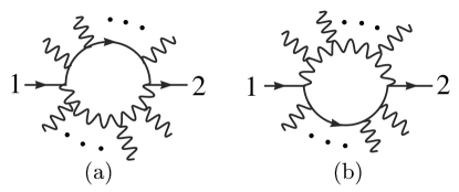
Figure 1: (a) An $L$ type primitive amplitude, in which the fermion line turns left on entering the loop (following the arrow). (b) In an $R$ type primitive amplitude, the fermion line turns right.

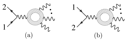
Figure 2: (a) Graphs in which the external fermion line passes to the left of the loop are assigned to $L$ type. (b) Graphs in which it passes to the right are called $R$ type. Gluons, fermions or scalars run in the loop. The same decomposition is used when gluons are emitted from the external fermion line.

Following ref. TwoQuarkThreeGluon , where more details can be found, we introduce the primitive amplitudes,

$$\matrix{&A_{n}^{L,[J]}(\phi,1_{\!f},3,4,\ldots,j,2_{\!f},j+1,\ldots,n),\hfill\cr&A_{n}^{R,[J]}(\phi,1_{\!f},3,4,\ldots,j,2_{\!f},j+1,\ldots,n),\hfill\cr}\hskip 28.45274ptJ=1,{\textstyle{1\over 2}}\displaystyle,0,$$ (23)

where $J={1\over 2}$ and $J=0$ denote the contributions with a closed fermion loop and closed complex scalar loop, respectively, and “$L$” and “$R$” denote the two orientations of the fermion line in the loop. Generic diagrams contributing to the $L$ and $R$ terms are shown in figs. 1 and 2. Because the primitive amplitudes can be used to build amplitudes with any color representation for the fermions, we label them by $f$ to denote a generic fermion in any color representation. Diagrams without closed fermion or scalar loops are assigned to $J=1$; they may or may not contain a closed gluon loop, as the two types of diagrams mix under gauge transformations. For notational simplicity, we suppress the superscript “$[1]$”, $A_{n}^{L}\equiv A_{n}^{L,[1]}\,,\,\,A_{n}^{R}\equiv A_{n}^{R,[1]}$. The primitive amplitudes (23) are not all independent. The set of diagrams where the incoming leg $1$ turns left is related, up to a sign, to a corresponding set where it turns right. Thus, the two sets are related by a reflection which reverses the cyclic ordering,

$$A_{n}^{R,[J]}(\phi,1_{\!f},3,4,\ldots,2_{\!f},\ldots,n-1,n)=(-1)^{n}A_{n}^{L,[J]}(\phi,1_{\!f},n,n-1,\ldots,2_{\!f},\ldots,4,3).$$ (24)

The leading-color contribution to eq. (21), $A_{n;1}$, is given in terms of primitive amplitudes by,

$$A_{n;1}(\phi,1_{\bar{q}},2_{q};3,\ldots,n) = A_{n}^{L}(\phi,1_{\!f},2_{\!f},3,\ldots,n)-{1\over N_{c}^{2}}A_{n}^{R}(\phi,1_{\!f},2_{\!f},3,\ldots,n)$$ (25)

$$+ {n_{\mskip-2.0muf}\over N_{c}}A_{n}^{L,[1/2]}(\phi,1_{\!f},2_{\!f},3,\ldots,n)+{n_{\mskip-2.0mus}\over N_{c}}A_{n}^{L,[0]}(\phi,1_{\!f},2_{\!f},3,\ldots,n).~{}~{}~{}~{}~{}~{}~{}$$

For QCD the number of scalars vanishes, $n_{\mskip-2.0mus}=0$, while $n_{\mskip-2.0muf}$ is the number of light quark flavors. The subleading-color partial amplitudes $A_{n;j>1}$ appearing in eq. (21) may be expressed as a permutation sum over primitive amplitudes,

$$\hskip-85.35826ptA_{n;j}(\phi,1_{\bar{q}},2_{q};3,\ldots,j+1;j+2,j+3,\ldots,n)$$ (26)

$$= (-1)^{j-1}\sum_{\sigma\in COP\{\alpha\}\{\beta\}}\Biggl{[}A_{n}^{L,[1]}(\phi,\sigma(1_{\!f},2_{\!f},3,\ldots,n))$$

$$-{n_{\mskip-2.0muf}\over N_{c}}A_{n}^{R,[1/2]}(\phi,\sigma(1_{\!f},2_{\!f},3,\ldots,n))-{n_{\mskip-2.0mus}\over N_{c}}A_{n}^{R,[0]}(\phi,\sigma(1_{\!f},2_{\!f},3,\ldots,n))\Biggr{]}\,,~{}~{}~{}~{}~{}~{}$$

where $\alpha_{i}\in\{\alpha\}\equiv\{j+1,j,\ldots,4,3\}$, $\beta_{i}\in\{\beta\}\equiv\{1,2,j+2,j+3,\ldots,n-1,n\}$, and $COP\{\alpha\}\{\beta\}$ is the set of all permutations of $\{1,2,\ldots,n\}$ defined after eq. (20), except that here leg $1$ is held fixed. However, as in the $n$-gluon case above, using $f^{abc}$-based color structures DDDM instead of trace-based ones, it is possible to avoid the introduction of the subleading-color amplitudes $A_{n;j>1}$.

In the case studied below, where all external gluons carry the same helicity, the fermion loop and scalar loop are the same up to a sign,

$$A_{n}^{L,[0]}(\phi,1_{\!f}^{-},2^{+},\ldots,j_{\!f}^{+},\ldots,n^{+}) = -A_{n}^{L,[1/2]}(\phi,1_{\!f}^{-},2^{+},\ldots,j_{\!f}^{+},\ldots,n^{+})$$ (27)

$$\equiv A_{n}^{s}(\phi,1_{\!f}^{-},2^{+},\ldots,j_{\!f}^{+},\ldots,n^{+})\,.$$

As mentioned above, in contrast to pure QCD, this relation does not follow from supersymmetry; instead we will show it recursively below. Then by computing the closed scalar-loop primitive amplitude we obtain also the closed fermion-loop primitive amplitude.

We shall find it convenient to compute the combinations

$$A_{n}^{s}\hskip 28.45274pt\hbox{and}\hskip 28.45274ptA_{n}^{L-s}\equiv A_{n}^{L}-A_{n}^{s}\,,$$ (28)

instead of $A_{n}^{s}$ and $A_{n}^{L}$. Also in contrast to pure QCD, for which an identity relates $A_{n}^{L-s}(1_{\!f}^{-},2^{+},\ldots,j_{\!f}^{+},\ldots,n^{+})$ with the amplitude with the cyclic ordering reversed, $A_{n}^{L-s}(1_{\!f}^{-},n^{+},\ldots,j_{\!f}^{+},\ldots,2^{+})$ LastFinite , here we will have to compute all $A_{n}^{L-s}$ for $j$ from 2 up to $n$. The generic recursion relation will only hold for $j\leq n-2$. However, we will be able to compute the cases of $A_{n}^{L-s}$ for $j=n$ or $j=n-1$ by taking collinear limits of appropriate amplitudes with larger $n$. The scalar-loop contribution $A_{n}^{s}$ vanishes if $j=n$ or $j=n-1$ — these configurations have only graphs with tadpoles and bubbles on external lines, which vanish in dimensional regularization.

In summary, for amplitudes with a single quark pair and identical-helicity gluon legs, there are two independent classes of primitive amplitudes to compute,

$$A_{n}^{L-s}(\phi,1_{\!f}^{-},2^{+},\ldots,j_{\!f}^{+},(j+1)^{+},\ldots,n^{+})\hskip 14.22636pt \hskip 14.22636ptA_{n}^{s}(\phi,1_{\!f}^{-},2^{+},\ldots,j_{\!f}^{+},(j+1)^{+},\ldots,n^{+})\,.$$ and

II.4 Spinor-helicity notation

The primitive amplitudes are functions of the massive momentum $k_{\phi}$ of the $\phi$ particle, and the massless momenta $k_{i}$ of the $n$ partons. All momenta entering the amplitudes are taken to be outgoing, so the kinematical constraints are,

$$k_{\phi}+\sum_{i=1}^{n}k_{i} = 0,$$ (29)

$$k_{\phi}^{2} = m_{H}^{2},\qquad k_{i}^{2}=0.$$ (30)

The amplitudes are best described using spinor inner-products SpinorHelicity ; TreeReview composed of the partonic momenta,

$$\left\langle j\,l\right\rangle=\langle j^{-}|l^{+}\rangle=\bar{u}_{-}(k_{j})u_{+}(k_{l})\,,\hskip 56.9055pt\left[j\,l\right]=\langle j^{+}|l^{-}\rangle=\bar{u}_{+}(k_{j})u_{-}(k_{l})\,,$$ (31)

where $u_{\pm}(k)$ is a massless Weyl spinor with momentum $k$ and positive or negative chirality. We use the convention $\left[j\,l\right]={\mathop{\rm sign}\nolimits}(k_{j}^{0}k_{l}^{0})\left\langle l\,j\right\rangle^{*}$ standard in the QCD literature, so that,

$$\left\langle i\,j\right\rangle\left[j\,i\right]=2k_{i}\cdot k_{j}\equiv s_{ij}\,.$$ (32)

We denote the sums of cyclicly-consecutive external momenta by

$$K^{\mu}_{i\cdots j}\equiv k_{i}^{\mu}+k_{i+1}^{\mu}+\cdots+k_{j-1}^{\mu}+k_{j}^{\mu},$$ (33)

where all indices are mod $n$ for an $n$-parton amplitude. The invariant mass of this vector is $s_{i\cdots j}\equiv K_{i\cdots j}^{2}$. Special cases include the two- and three-particle invariant masses, which are denoted by

$$s_{ij}\equiv K_{i,j}^{2}\equiv(k_{i}+k_{j})^{2}=2k_{i}\cdot k_{j},\qquad\quad s_{ijk}\equiv(k_{i}+k_{j}+k_{k})^{2}.$$ (34)

In color-ordered amplitudes only invariants with cyclicly-consecutive arguments need appear, e.g. $s_{i,i+1}$ and $s_{i,i+1,i+2}$. It is convenient to introduce the same combinations as eq. (33) but with the $\phi$ momentum added as well,

$$K^{\mu}_{\phi,i\cdots j}\equiv k_{\phi}^{\mu}+k_{i}^{\mu}+k_{i+1}^{\mu}+\cdots+k_{j-1}^{\mu}+k_{j}^{\mu},$$ (35)

with invariant-mass $s_{\phi,i\cdots j}\equiv K_{\phi,i\cdots j}^{2}$. Longer spinor strings will also appear, such as

$$\left\langle\smash{k}{\vphantom{1}}^{-}\right|{{\raise 0.91666pt\hbox to9.20833pt{\hss/\hss}\hbox to0.0pt{\hss$K$}}_{i\cdots j}}\left|\smash{l}{\vphantom{1}}^{-}\right\rangle = \sum_{m=i}^{j}\left\langle k\,m\right\rangle\left[m\,l\right]\,,$$ (36)

$$\left\langle\smash{k}{\vphantom{1}}^{-}\right|{{\raise 0.91666pt\hbox to9.20833pt{\hss/\hss}\hbox to0.0pt{\hss$K$}}_{i_{1}\cdots j_{1}}{\raise 0.91666pt\hbox to9.20833pt{\hss/\hss}\hbox to0.0pt{\hss$K$}}_{i_{2}\cdots j_{2}}}\left|\smash{l}{\vphantom{1}}^{+}\right\rangle = \sum_{m_{1}=i_{1}}^{j_{1}}\sum_{m_{2}=i_{2}}^{j_{2}}\left\langle k\,m_{1}\right\rangle\left[m_{1}\,m_{2}\right]\left\langle m_{2}\,l\right\rangle\,.$$ (37)

For small values of $n$, such strings can be written out explicitly as

$$\left\langle\smash{k}{\vphantom{1}}^{-}\right|{(a+b)}\left|\smash{l}{\vphantom{1}}^{-}\right\rangle = \left\langle k\,a\right\rangle\left[a\,l\right]+\left\langle k\,b\right\rangle\left[b\,l\right]\,,$$

$$\left\langle\smash{k}{\vphantom{1}}^{+}\right|{(a+b)}\left|\smash{l}{\vphantom{1}}^{+}\right\rangle = \left[k\,a\right]\left\langle a\,l\right\rangle+\left[k\,b\right]\left\langle b\,l\right\rangle\,,$$

$$\left\langle\smash{k}{\vphantom{1}}^{-}\right|{(a+b)(c+d)}\left|\smash{l}{\vphantom{1}}^{+}\right\rangle = \left\langle k\,a\right\rangle\left\langle\smash{a}{\vphantom{1}}^{+}\right|{(c+d)}\left|\smash{l}{\vphantom{1}}^{+}\right\rangle+\left\langle k\,b\right\rangle\left\langle\smash{b}{\vphantom{1}}^{+}\right|{(c+d)}\left|\smash{l}{\vphantom{1}}^{+}\right\rangle\,.$$ (38)

III Review of recursion relations and factorization

III.1 On-shell recursion relations

Here we briefly review the on-shell recursion relations found and proved in refs. BCFRecursion ; BCFW . For further details we refer to these papers. The on-shell recursion relations rely on general properties of complex functions as well as factorization properties of scattering amplitudes. The proof BCFW of the relations relies on a parameter-dependent “$[k,l\rangle$” shift of two of the external massless spinors, $k$ and $l$, in an $n$-point process,

$$[k,l\rangle:\quad\quad{\tilde{\lambda}}_{k}\rightarrow{\tilde{\lambda}}_{k}-z{\tilde{\lambda}}_{l}\,,\qquad\quad\lambda_{l}\rightarrow\lambda_{l}+z\lambda_{k}\,,$$ (39)

where $z$ is a complex number. The corresponding momenta (labeled by $p_{i}$ instead of $k_{i}$ in this section) are shifted as well,

$$p_{k}^{\mu} \rightarrow\ p_{k}^{\mu}(z)=p_{k}^{\mu}-{z\over 2}{\left\langle\smash{k}{\vphantom{1}}^{-}\right|{\gamma^{\mu}}\left|\smash{l}{\vphantom{1}}^{-}\right\rangle},$$ (40)

$$p_{l}^{\mu} \rightarrow\ p_{l}^{\mu}(z)=p_{l}^{\mu}+{z\over 2}{\left\langle\smash{k}{\vphantom{1}}^{-}\right|{\gamma^{\mu}}\left|\smash{l}{\vphantom{1}}^{-}\right\rangle}\,,$$

so that they remain massless, $p_{k}^{2}(z)=0=p_{l}^{2}(z)$, and overall momentum conservation is maintained.

An on-shell amplitude containing the momenta $p_{k}$ and $p_{l}$ then becomes parameter-dependent as well,

$$A(z)=A(p_{1},\ldots,p_{k}(z),p_{k+1},\ldots,p_{l}(z),p_{l+1},\ldots,p_{n}).$$ (41)

When $A$ is a tree amplitude or finite one-loop amplitude, $A(z)$ is a rational function of $z$. The physical amplitude is given by $A(0)$.

If $A(z)\rightarrow 0$ as $z\rightarrow\infty$, as in suitable cases in tree-level QCD BCFRecursion ; BCFW ; LuoWen ; BadgerMassive , then the contour integral around the circle $C$ at infinity vanishes,

$${1\over 2\pi i}\oint_{C}{dz\over z}\,A(z)=0\,;$$ (42)

that is, there is no “surface term”. In appendix B we show that a tree amplitude $A(z)$ containing an extra $\phi$ field also vanishes as $z\rightarrow\infty$, for the same choices of shift that lead to a vanishing $A(z)$ in pure QCD.

Evaluating the integral (42) as a sum of residues, we can then solve for $A(0)$ to obtain,

$$A(0)=-\sum_{{\rm poles}\ \alpha}\mathop{\rm Res}_{z=z_{\alpha}}{A(z)\over z}\,.$$ (43)

If $A(z)$ only has simple poles, then each residue is given by factorizing the shifted amplitude on the appropriate pole in momentum invariants BCFW , so that at tree level,

$$A(0)=\sum_{r,s,h}A^{h}_{L}(z=z_{rs}){i\over K_{r\cdots s}^{2}}A^{-h}_{R}(z=z_{rs})\,,$$ (44)

where $h=\pm 1$ labels the helicity of the intermediate state. There is generically a double sum over momentum poles, labeled by leg indices $r,s$, with legs $k$ and $l$ always appearing on opposite sides of the pole. By definition, the leg $l$ is contained in the set $\{r,\ldots,s\}$ and the leg $k$ is not. The squared momentum associated with the pole, $K_{r\cdots s}^{2}$, is evaluated in the unshifted kinematics; whereas the on-shell amplitudes $A_{L}$ and $A_{R}$ are evaluated in kinematics that have been shifted by eq. (39) with $z=z_{rs}$, where

$$z_{rs}=-{K_{r\cdots s}^{2}\over\left\langle\smash{k}{\vphantom{1}}^{-}\right|{{\raise 0.91666pt\hbox to9.20833pt{\hss/\hss}\hbox to0.0pt{\hss$K$}}_{r\ldots s}}\left|\smash{l}{\vphantom{1}}^{-}\right\rangle}\,.$$ (45)

To extend the approach to one loop OnShellRecursionI , the sum (44) should also be taken over the two ways of assigning the loop to $A_{L}$ and $A_{R}$. This formula assumes that there are no additional poles present in the amplitude other than the standard poles for real momenta. At tree level it is possible to demonstrate the absence of additional poles, but at loop level it is not true.

Because of the general structure of multiparticle factorization BernChalmers , only standard single poles in $z$ arise from multiparticle channels, even at one loop. However, double poles in $z$ do arise at one loop due to collinear factorization OnShellRecursionI ; BBDFK1 . The splitting amplitudes with helicity configuration $(+{}+{}+)$ and $(-{}-{}-)$ (in an all-outgoing helicity convention) can lead to double poles in $z$, because their dependence on the spinor products takes the form $\left[a\,b\right]/\left\langle a\,b\right\rangle^{2}$ for $(+{}+{}+)$, or its complex conjugate $\left\langle a\,b\right\rangle/\left[a\,b\right]^{2}$ for $(-{}-{}-)$ Neq4Oneloop . As discussed in ref. OnShellRecursionI , this behavior alters the form of the recursion relation in an essential manner. In general, underneath the double pole sits an object of the form,

$${\left[a\,b\right]\over\left\langle a\,b\right\rangle}\,,$$ (46)

which we call an “unreal pole” because there is no pole present when real momenta are used; it only appears, as a single pole, when we continue to complex momenta. As we shall discuss in section VII, the finite $\phi\bar{q}qgg\ldots g$ amplitudes exhibit similar phenomena, except that in this case, just as in the pure-QCD case of finite $\bar{q}qgg\ldots g$ amplitudes LastFinite , one encounters unreal poles that do not sit underneath a double pole.

III.2 One-loop factorization properties

In order to build on-shell recursion relations, we need the factorization properties of one-loop amplitudes for complex momenta. It is useful to first review the factorization properties for real momenta, which we know from general arguments TreeReview ; BernChalmers ; OneloopSplit .

As the real momenta of two color-adjacent external partons $a$ and $b$ become collinear, the one-loop amplitude factorizes as,

$$A_{n}^{{(1)}}\buildrel a\parallel b\over{\relbar\mskip-0.5mu\joinrel\mskip-0.5mu\relbar\mskip-0.5mu\joinrel\longrightarrow}\ \sum_{h=\pm} \hbox{}\hskip-9.95863pt\biggl{(}\mathop{\rm Split}\nolimits^{(0)}_{-h}(a^{h_{a}},b^{h_{b}};z)\,A_{n-1}^{{(1)}}(\ldots,(a+b)^{h},\ldots)$$ (47)

$$\hphantom{\biggl{(})}+\mathop{\rm Split}\nolimits^{{(1)}}_{-h}(a^{h_{a}},b^{h_{b}};z)\,A_{n-1}^{(0)}(\ldots,(a+b)^{h},\ldots)\biggr{)}\,.$$

The tree and loop splitting amplitudes $\mathop{\rm Split}\nolimits^{(0)}$ and $\mathop{\rm Split}\nolimits^{{(1)}}$ are given in ref. Neq4Oneloop . In general, there are three types of limits: a pair of gluons becoming collinear; a gluon becoming collinear with a quark (or anti-quark); and a quark and anti-quark becoming collinear (if they happen to be adjacent). When all external gluons have positive helicity, as here, the limits simplify. For $\phi$-amplitudes, no singularity results when a parton becomes collinear with the $\phi$ state, because the $\phi$ is massive.

When two gluons become collinear, the finite $\phi\bar{q}qgg\ldots g$ amplitudes $A_{n}^{L}$ and $A_{n}^{s}$ behave respectively as,

$$A_{n}^{L}(\phi,\ldots,a^{+},b^{+},\ldots)\buildrel a\parallel b\over{\relbar\mskip-0.5mu\joinrel\mskip-0.5mu\relbar\mskip-0.5mu\joinrel\longrightarrow}\ \mathop{\rm Split}\nolimits^{(0)}_{-}(a^{+},b^{+};z)\,A_{n-1}^{L}(\phi,\ldots,(a+b)^{+},\ldots)$$ (48)

$$+\mathop{\rm Split}\nolimits^{{(1)}:g}_{+}(a^{+},b^{+};z)\,A_{n-1}^{(0)}(\phi,\ldots,(a+b)^{-},\ldots)\,,$$

$$A_{n}^{s}(\phi,\ldots,a^{+},b^{+},\ldots)\buildrel a\parallel b\over{\relbar\mskip-0.5mu\joinrel\mskip-0.5mu\relbar\mskip-0.5mu\joinrel\longrightarrow}\ \mathop{\rm Split}\nolimits^{(0)}_{-}(a^{+},b^{+};z)\,A_{n-1}^{s}(\phi,\ldots,(a+b)^{+},\ldots)$$ (49)

$$+\mathop{\rm Split}\nolimits^{{(1)}:s}_{+}(a^{+},b^{+};z)\,A_{n-1}^{(0)}(\phi,\ldots,(a+b)^{-},\ldots)\,.$$

Here $\mathop{\rm Split}\nolimits^{{(1)}:g}$ ($\mathop{\rm Split}\nolimits^{{(1)}:s}$) is the one-loop splitting amplitude with a gluon (scalar) circulating in the loop. The remaining two terms, with opposite intermediate-gluon helicity, vanish because $\mathop{\rm Split}\nolimits^{(0)}_{+}(a^{+},b^{+};z)$ and $A_{n-1}^{(0)}(\phi,\pm,+,+,\ldots,+)$ are zero. Because the two one-loop splitting amplitudes are equal Neq4Oneloop ,

$$\mathop{\rm Split}\nolimits^{{(1)}:g}_{+}(a^{+},b^{+};z)=\mathop{\rm Split}\nolimits^{{(1)}:s}_{+}(a^{+},b^{+};z),$$ (50)

we are motivated to take the difference between $A_{n}^{L}$ and $A_{n}^{s}$ to form $A_{n}^{L-s}$. This combination has the simpler collinear behavior,

$$A_{n}^{L-s}(\phi,\ldots,a^{+},b^{+},\ldots)\buildrel a\parallel b\over{\relbar\mskip-0.5mu\joinrel\mskip-0.5mu\relbar\mskip-0.5mu\joinrel\longrightarrow}\ \mathop{\rm Split}\nolimits^{(0)}_{-}(a^{+},b^{+};z)\,A_{n-1}^{L-s}(\phi,\ldots,(a+b)^{+},\ldots)\,.$$ (51)

When a gluon becomes collinear with any fermion, both $A_{n}^{L}$ and $A_{n}^{s}$ behave as (using fermion helicity-conservation and eq. (77)),

$$A_{n}^{L,s}(\phi,a_{\!f}^{\pm},b^{+},\ldots)\buildrel a\parallel b\over{\relbar\mskip-0.5mu\joinrel\mskip-0.5mu\relbar\mskip-0.5mu\joinrel\longrightarrow}\mathop{\rm Split}\nolimits^{(0)}_{(f)\mp}(a_{\!f}^{\pm},b^{+};z)\,A_{n-1}^{L,s}(\phi,(a+b)_{\!f}^{\pm},\ldots)\,.$$ (52)

Hence the difference $A_{n}^{L-s}$ has the limiting behavior,

$$A_{n}^{L-s}(\phi,a_{\!f}^{\pm},b^{+},\ldots)\buildrel a\parallel b\over{\relbar\mskip-0.5mu\joinrel\mskip-0.5mu\relbar\mskip-0.5mu\joinrel\longrightarrow}\mathop{\rm Split}\nolimits^{(0)}_{(f)\mp}(a_{\!f}^{\pm},b^{+};z)\,A_{n-1}^{L-s}(\phi,(a+b)_{\!f}^{\pm},\ldots)\,.$$ (53)

When a quark and anti-quark become collinear (for $j_{\!f}=2$), the amplitude factorizes onto the finite one-loop $\phi gg\ldots g$ amplitudes,

$$A_{n}^{L,s}(\phi,a_{\!f}^{-},b_{\!f}^{+},\ldots)\buildrel a\parallel b\over{\relbar\mskip-0.5mu\joinrel\mskip-0.5mu\relbar\mskip-0.5mu\joinrel\longrightarrow}\ \mathop{\rm Split}\nolimits^{(0)}_{-}(a_{\!f}^{-},b_{\!f}^{+};z)\,A_{n-1}^{[g,s]}(\phi,(a+b)^{+},\ldots)$$ (54)

$$\hbox{}+\mathop{\rm Split}\nolimits^{(0)}_{+}(a_{\!f}^{-},b_{\!f}^{+};z)\,A_{n-1}^{[g,s]}(\phi,(a+b)^{-},\ldots)\,.$$

As mentioned in section II.3, in contrast with the pure-QCD case LastFinite , the gluon and scalar loop contributions to $A_{n-1;1}(\phi,\pm,+,+,\ldots,+)$ are not the same. For the difference $A_{n}^{L-s}$ we find from eq. (54) the collinear behavior,

$$A_{n}^{L-s}(\phi,a_{\!f}^{-},b_{\!f}^{+},\ldots)\buildrel a\parallel b\over{\relbar\mskip-0.5mu\joinrel\mskip-0.5mu\relbar\mskip-0.5mu\joinrel\longrightarrow}\ \mathop{\rm Split}\nolimits^{(0)}_{-}(a_{\!f}^{-},b_{\!f}^{+};z)\,A_{n-1}^{[g-s]}(\phi,(a+b)^{+},\ldots)$$ (55)

$$\hbox{}+\mathop{\rm Split}\nolimits^{(0)}_{+}(a_{\!f}^{-},b_{\!f}^{+};z)\,A_{n-1}^{[g-s]}(\phi,(a+b)^{-},\ldots)\,.$$

Next consider multiparticle factorization. In this case, the vanishing of the tree amplitudes $A_{n}^{(0)}(1_{\!f}^{-},2^{+},\ldots,j_{\!f}^{+},\ldots,n^{+})$ and $A_{n}^{(0)}(\phi,1_{\!f}^{-},2^{+},\ldots,j_{\!f}^{+},\ldots,n^{+})$ means that the only singularities are on gluon poles. There are two possible ways to attach the $\phi$ field,

$$\hbox{}\hskip-11.38109ptA_{n}^{L,s}(\phi,1_{\!f}^{-},2^{+},\ldots,j_{\!f}^{+},\ldots,m^{+},\ldots,n^{+})\buildrel K_{1\cdots m}^{2}\rightarrow 0\over{\relbar\mskip-0.5mu\joinrel\mskip-0.5mu\relbar\mskip-0.5mu\joinrel\longrightarrow}$$ (56)

$$\hskip 14.22636ptA_{m+1}^{(0)}(\phi,1_{\!f}^{-},2^{+},\ldots,j_{\!f}^{+},\ldots,m^{+},-K_{1\ldots m}^{-}){i\over K_{1\ldots m}^{2}}A_{n-m+1}^{{(1)}}(K_{1\ldots m}^{+},(m+1)^{+},\ldots,n^{+})\,$$

$$\hskip 14.22636pt+\ A_{m+1}^{(0)}(1_{\!f}^{-},2^{+},\ldots,j_{\!f}^{+},\ldots,m^{+},-K_{1\ldots m}^{-}){i\over K_{1\ldots m}^{2}}A_{n-m+1}^{[g,s]}(\phi,K_{1\ldots m}^{+},(m+1)^{+},\ldots,n^{+})\,,$$

with $m\geq 3$ and $m\geq j_{\!f}$. For $A_{n}^{L-s}$, the first term in eq. (56) does not contribute, but the second does.

In addition to the factorization properties for real momenta just described, the appearance of unreal poles of the form (46) sometimes has to be taken into account. While such behavior is not understood in general, in the present case we can use the similarity of our amplitudes to the corresponding finite pure-QCD amplitudes $\bar{q}qgg\ldots g$ LastFinite . The contribution of unreal-pole terms to the recursion relations for those amplitudes could be stringently cross checked against various QCD and QED amplitudes. The inclusion of a massive $\phi$ field is quite mild from the point of view of factorization, so it should not alter the form of the unreal-pole terms in the recursion relations. In section VII we will describe these terms in more detail.

IV Review of known finite amplitudes

In this section, we collect previously-known results for tree and one-loop finite amplitudes in pure QCD, and for tree amplitudes containing a single $\phi$ field. These results feed into the recursive formulæ for the finite one-loop amplitudes containing a single $\phi$ field, to be discussed in section VII.

IV.1 Pure-QCD amplitudes

The $n$-gluon tree amplitudes with zero or one negative-helicity gluon all vanish,

$$A_{n}^{(0)}(1^{\pm},2^{+},3^{+},\ldots,n^{+})=0\,,$$ (57)

where the omitted labels (“$\ldots$”) always refer to positive-helicity gluons. Also vanishing are the tree amplitudes for a pair of massless quarks and $(n-2)$ gluons all of the same helicity,

$$A_{n}^{(0)}(1_{\!f}^{-},2^{+},\ldots,(j-1)^{+},j_{\!f}^{+},(j+1)^{+},\ldots,n^{+})=0\,,$$ (58)

where the subscript $f$ denotes a generic fermion, and the positive-helicity fermion ($j_{\!f}^{+}$) can be located at an arbitrary position with respect to the negative-helicity one ($1_{\!f}^{-}$). (Note that only the case $j=2$ is required in the pure-QCD version of the tree-level formula (10).)

The first nonvanishing tree amplitudes are the MHV amplitudes ParkeTaylor ; TreeReview ,

$$A_{n}^{(0)}(1^{+},2^{+},\ldots,m_{1}^{-},\ldots,m_{2}^{-},\ldots,n^{+})=i{\left\langle m_{1}\,m_{2}\right\rangle^{4}\over\left\langle 1\,2\right\rangle\left\langle 2\,3\right\rangle\cdots\left\langle n\,1\right\rangle}\,,$$ (59)

and

$$A_{n}^{(0)}(1_{\!f}^{-},2^{+},\ldots,j_{\!f}^{+},\ldots,m^{-},\ldots,n^{+})=i{\left\langle 1\,m\right\rangle^{3}\left\langle j\,m\right\rangle\over\left\langle 1\,2\right\rangle\left\langle 2\,3\right\rangle\cdots\left\langle n\,1\right\rangle}\,.$$ (60)

We also need the one-loop pure-gluon amplitudes with zero or one negative helicity. The all-positive-helicity case, for $n\geq 4$, is given by AllPlus ; Mahlon

$$A_{n}^{[g]}(1^{+},2^{+},\ldots,n^{+})=A_{n}^{[s]}(1^{+},2^{+},\ldots,n^{+})={i\over 3}{H_{n}\over\left\langle 1\,2\right\rangle\left\langle 2\,3\right\rangle\cdots\left\langle(n-1)\,n\right\rangle\left\langle n\,1\right\rangle}\,,$$ (61)

where

$$H_{n}=-\sum_{1\leq i_{1}<i_{2}<i_{3}<i_{4}\leq n}\,{\rm Tr}_{-}\Bigl{[}{\raise 0.97221pt\hbox to5.52084pt{\hss/\hss}\hbox to0.0pt{\hss$k$}}_{i_{1}}{\raise 0.97221pt\hbox to5.52084pt{\hss/\hss}\hbox to0.0pt{\hss$k$}}_{i_{2}}{\raise 0.97221pt\hbox to5.52084pt{\hss/\hss}\hbox to0.0pt{\hss$k$}}_{i_{3}}{\raise 0.97221pt\hbox to5.52084pt{\hss/\hss}\hbox to0.0pt{\hss$k$}}_{i_{4}}\Bigr{]}\,,$$ (62)

and

$$\,{\rm Tr}_{-}\Bigl{[}{\raise 0.97221pt\hbox to5.52084pt{\hss/\hss}\hbox to0.0pt{\hss$k$}}_{i_{1}}{\raise 0.97221pt\hbox to5.52084pt{\hss/\hss}\hbox to0.0pt{\hss$k$}}_{i_{2}}{\raise 0.97221pt\hbox to5.52084pt{\hss/\hss}\hbox to0.0pt{\hss$k$}}_{i_{3}}{\raise 0.97221pt\hbox to5.52084pt{\hss/\hss}\hbox to0.0pt{\hss$k$}}_{i_{4}}\Bigr{]} = {1\over 2}\,{\rm Tr}[(1-\gamma_{5}){\raise 0.97221pt\hbox to5.52084pt{\hss/\hss}\hbox to0.0pt{\hss$k$}}_{i_{1}}{\raise 0.97221pt\hbox to5.52084pt{\hss/\hss}\hbox to0.0pt{\hss$k$}}_{i_{2}}{\raise 0.97221pt\hbox to5.52084pt{\hss/\hss}\hbox to0.0pt{\hss$k$}}_{i_{3}}{\raise 0.97221pt\hbox to5.52084pt{\hss/\hss}\hbox to0.0pt{\hss$k$}}_{i_{4}}]$$ (63)

$$= \left\langle i_{1}\,i_{2}\right\rangle\left[i_{2}\,i_{3}\right]\left\langle i_{3}\,i_{4}\right\rangle\left[i_{4}\,i_{1}\right]\,.$$

It is convenient to rewrite eq. (61) using an identity proved in ref. LastFinite ,

$$H_{n}=-{1\over 2}\,{\rm Tr}_{-}[{\cal F}(2,n)]^{2}\,,$$ (64)

where we define the more general quantity ${\cal F}(l,p)$,

$${\cal F}(l,p)=\sum_{i=l}^{p-1}\sum_{m=i+1}^{p}{\raise 0.97221pt\hbox to5.52084pt{\hss/\hss}\hbox to0.0pt{\hss$k$}}_{i}{\raise 0.97221pt\hbox to5.52084pt{\hss/\hss}\hbox to0.0pt{\hss$k$}}_{m}\,,$$ (65)

involving sums over ordered pairs ($i<m$) of momenta between $l$ and $p$. In eq. (64) for the $n$-point all-plus amplitude, all such pairs appear except those involving leg 1. Using the cyclic symmetry of this amplitude, any one of the $n$ legs could be omitted, say leg $l$, if the ordering in the corresponding sums for ${\cal F}(l+1,l-1)$ is defined modulo $n$ in eq. (65).

For $n=3$ we need to take one leg off shell. We define a vertex, with legs $1$ and $2$ the on-shell external legs OnShellRecursionI ,

$$A_{3}^{(1)}(1^{+},2^{+},3^{+}) = {V_{3}^{(1)}(1^{+},2^{+},3^{+})\over K_{1,2}^{2}}\,,$$ (66)

where

$$V_{3}^{(1)}(1^{+},2^{+},3^{+})\equiv-{i\over 3}\left[1\,2\right]\left[2\,3\right]\left[3\,1\right]\,.$$ (67)

The remaining one-loop finite helicity amplitudes in pure QCD are those for $n$ gluons, with one of negative helicity; and those for a quark-antiquark pair plus $(n-2)$ gluons of positive helicity. They are not actually needed for the recursion relations for the single-$\phi$ amplitudes considered here. However, their structure, in the form given in ref. LastFinite , is so similar to that of the single-$\phi$ amplitudes, that we reproduce them here. The one-minus $n$-gluon amplitude is given by,

$$A_{n;1}(1^{-},2^{+},3^{+},\ldots,n^{+})={i\over 3}{T_{1}+T_{2}\over\left\langle 1\,2\right\rangle\left\langle 2\,3\right\rangle\cdots\left\langle n\,1\right\rangle}\,,$$ (68)

where

$$T_{1} = \sum_{l=2}^{n-1}{\left\langle 1\,l\right\rangle\left\langle 1\,(l+1)\right\rangle\left\langle\smash{1}{\vphantom{1}}^{-}\right|{{\raise 0.91666pt\hbox to9.20833pt{\hss/\hss}\hbox to0.0pt{\hss$K$}}_{l,l+1}{\raise 0.91666pt\hbox to9.20833pt{\hss/\hss}\hbox to0.0pt{\hss$K$}}_{(l+1)\cdots n}}\left|\smash{1}{\vphantom{1}}^{+}\right\rangle\over\left\langle l\,(l+1)\right\rangle}\,,$$ (69)

$$T_{2} = \sum_{l=3}^{n-2}\sum_{p=l+1}^{n-1}{\left\langle(l-1)\,l\right\rangle\over\left\langle\smash{1}{\vphantom{1}}^{-}\right|{{\raise 0.91666pt\hbox to9.20833pt{\hss/\hss}\hbox to0.0pt{\hss$K$}}_{(p+1)\cdots n}{\raise 0.91666pt\hbox to9.20833pt{\hss/\hss}\hbox to0.0pt{\hss$K$}}_{l\cdots p}}\left|\smash{(l-1)}{\vphantom{1}}^{+}\right\rangle\left\langle\smash{1}{\vphantom{1}}^{-}\right|{{\raise 0.91666pt\hbox to9.20833pt{\hss/\hss}\hbox to0.0pt{\hss$K$}}_{(p+1)\cdots n}{\raise 0.91666pt\hbox to9.20833pt{\hss/\hss}\hbox to0.0pt{\hss$K$}}_{l\cdots p}}\left|\smash{l}{\vphantom{1}}^{+}\right\rangle}$$ (70)

$$\hskip 42.67912pt\times{\left\langle p\,(p+1)\right\rangle\over\left\langle\smash{1}{\vphantom{1}}^{-}\right|{{\raise 0.91666pt\hbox to9.20833pt{\hss/\hss}\hbox to0.0pt{\hss$K$}}_{2\cdots(l-1)}{\raise 0.91666pt\hbox to9.20833pt{\hss/\hss}\hbox to0.0pt{\hss$K$}}_{l\cdots p}}\left|\smash{p}{\vphantom{1}}^{+}\right\rangle\left\langle\smash{1}{\vphantom{1}}^{-}\right|{{\raise 0.91666pt\hbox to9.20833pt{\hss/\hss}\hbox to0.0pt{\hss$K$}}_{2\cdots(l-1)}{\raise 0.91666pt\hbox to9.20833pt{\hss/\hss}\hbox to0.0pt{\hss$K$}}_{l\cdots p}}\left|\smash{(p+1)}{\vphantom{1}}^{+}\right\rangle}$$

$$\hskip 42.67912pt\times{\left\langle\smash{1}{\vphantom{1}}^{-}\right|{{\raise 0.91666pt\hbox to9.20833pt{\hss/\hss}\hbox to0.0pt{\hss$K$}}_{l\cdots p}{\raise 0.91666pt\hbox to9.20833pt{\hss/\hss}\hbox to0.0pt{\hss$K$}}_{(p+1)\cdots n}}\left|\smash{1}{\vphantom{1}}^{+}\right\rangle}^{3}$$

$$\hskip 42.67912pt\times{\left\langle\smash{1}{\vphantom{1}}^{-}\right|{{\raise 0.91666pt\hbox to9.20833pt{\hss/\hss}\hbox to0.0pt{\hss$K$}}_{2\cdots(l-1)}[{\cal F}(l,p)]^{2}{\raise 0.91666pt\hbox to9.20833pt{\hss/\hss}\hbox to0.0pt{\hss$K$}}_{(p+1)\cdots n}}\left|\smash{1}{\vphantom{1}}^{+}\right\rangle\over s_{l\cdots p}}\,.$$

The finite one-loop QCD amplitudes with quarks are LastFinite ,

$$A_{n}^{L-s}(1_{\!f}^{-},2^{+},\ldots,j_{\!f}^{+},\ldots,n^{+})={i\over 2}{Q_{0}\over\left\langle 1\,2\right\rangle\left\langle 2\,3\right\rangle\cdots\left\langle n\,1\right\rangle}\,,$$ (71)

where

$$Q_{0}=\left\langle 1\,j\right\rangle\sum_{l=3}^{n-1}\left\langle\smash{1}{\vphantom{1}}^{-}\right|{{\raise 0.91666pt\hbox to9.20833pt{\hss/\hss}\hbox to0.0pt{\hss$K$}}_{2\cdots l}{\raise 0.97221pt\hbox to5.52084pt{\hss/\hss}\hbox to0.0pt{\hss$k$}}_{l}}\left|\smash{1}{\vphantom{1}}^{+}\right\rangle\,,$$ (72)

and

$$A_{n}^{s}(1_{\!f}^{-},2^{+},\ldots,j_{\!f}^{+},\ldots,n^{+})={i\over 3}{S_{1}+S_{2}\over\left\langle 1\,2\right\rangle\left\langle 2\,3\right\rangle\cdots\left\langle n\,1\right\rangle}\,,$$ (73)

where

$$S_{1} = \sum_{l=j+1}^{n-1}{\left\langle j\,l\right\rangle\left\langle 1\,(l+1)\right\rangle\left\langle\smash{1}{\vphantom{1}}^{-}\right|{{\raise 0.91666pt\hbox to9.20833pt{\hss/\hss}\hbox to0.0pt{\hss$K$}}_{l,l+1}{\raise 0.91666pt\hbox to9.20833pt{\hss/\hss}\hbox to0.0pt{\hss$K$}}_{(l+1)\cdots n}}\left|\smash{1}{\vphantom{1}}^{+}\right\rangle\over\left\langle l\,(l+1)\right\rangle}\,,$$ (74)

$$S_{2} = \sum_{l=j+1}^{n-2}\sum_{p=l+1}^{n-1}{\left\langle(l-1)\,l\right\rangle\over\left\langle\smash{1}{\vphantom{1}}^{-}\right|{{\raise 0.91666pt\hbox to9.20833pt{\hss/\hss}\hbox to0.0pt{\hss$K$}}_{(p+1)\cdots n}{\raise 0.91666pt\hbox to9.20833pt{\hss/\hss}\hbox to0.0pt{\hss$K$}}_{l\cdots p}}\left|\smash{(l-1)}{\vphantom{1}}^{+}\right\rangle\left\langle\smash{1}{\vphantom{1}}^{-}\right|{{\raise 0.91666pt\hbox to9.20833pt{\hss/\hss}\hbox to0.0pt{\hss$K$}}_{(p+1)\cdots n}{\raise 0.91666pt\hbox to9.20833pt{\hss/\hss}\hbox to0.0pt{\hss$K$}}_{l\cdots p}}\left|\smash{l}{\vphantom{1}}^{+}\right\rangle}$$ (75)

$$\hskip 42.67912pt\times{\left\langle p\,(p+1)\right\rangle\over\left\langle\smash{1}{\vphantom{1}}^{-}\right|{{\raise 0.91666pt\hbox to9.20833pt{\hss/\hss}\hbox to0.0pt{\hss$K$}}_{2\cdots(l-1)}{\raise 0.91666pt\hbox to9.20833pt{\hss/\hss}\hbox to0.0pt{\hss$K$}}_{l\cdots p}}\left|\smash{p}{\vphantom{1}}^{+}\right\rangle\left\langle\smash{1}{\vphantom{1}}^{-}\right|{{\raise 0.91666pt\hbox to9.20833pt{\hss/\hss}\hbox to0.0pt{\hss$K$}}_{2\cdots(l-1)}{\raise 0.91666pt\hbox to9.20833pt{\hss/\hss}\hbox to0.0pt{\hss$K$}}_{l\cdots p}}\left|\smash{(p+1)}{\vphantom{1}}^{+}\right\rangle}$$

$$\hskip 42.67912pt\times{\left\langle\smash{1}{\vphantom{1}}^{-}\right|{{\raise 0.91666pt\hbox to9.20833pt{\hss/\hss}\hbox to0.0pt{\hss$K$}}_{l\cdots p}{\raise 0.91666pt\hbox to9.20833pt{\hss/\hss}\hbox to0.0pt{\hss$K$}}_{(p+1)\cdots n}}\left|\smash{1}{\vphantom{1}}^{+}\right\rangle}^{2}\left\langle\smash{j}{\vphantom{1}}^{-}\right|{{\raise 0.91666pt\hbox to9.20833pt{\hss/\hss}\hbox to0.0pt{\hss$K$}}_{l\cdots p}{\raise 0.91666pt\hbox to9.20833pt{\hss/\hss}\hbox to0.0pt{\hss$K$}}_{(p+1)\cdots n}}\left|\smash{1}{\vphantom{1}}^{+}\right\rangle$$

$$\hskip 42.67912pt\times{\left\langle\smash{1}{\vphantom{1}}^{-}\right|{{\raise 0.91666pt\hbox to9.20833pt{\hss/\hss}\hbox to0.0pt{\hss$K$}}_{2\cdots(l-1)}[{\cal F}(l,p)]^{2}{\raise 0.91666pt\hbox to9.20833pt{\hss/\hss}\hbox to0.0pt{\hss$K$}}_{(p+1)\cdots n}}\left|\smash{1}{\vphantom{1}}^{+}\right\rangle\over s_{l\cdots p}}\,.$$

These expressions coincide for $n=4,5$ with previously-computed amplitudes KunsztEtAl ; GGGGG ; TwoQuarkThreeGluon . Equation (68) agrees numerically with the result of ref. Mahlon for $n\leq 18$. Furthermore, in ref. LastFinite the amplitudes (71) and (73) were related to QED and mixed QED/QCD amplitudes by converting gluons into photons using appropriate permutation sums TwoQuarkThreeGluon . The resulting amplitudes can be compared to the one-loop QED and mixed photon-gluon amplitudes computed by Mahlon Mahlon ; MahlonQED , which provides a strong cross check of eqs. (71) and (73), and of the recursion relations used to generate them.

IV.2 Amplitudes with a $\phi$ field

Amplitudes containing a single $\phi$ field have an “MHV structure” very close to that of pure QCD DGK ; BGK . First of all, those helicity configurations with almost all positive-helicity gluons, which vanish in tree-level QCD, eqs. (57) and (58), continue to vanish when a single $\phi$ is added,

$$A_{n}^{(0)}(\phi,1^{\pm},2^{+},3^{+},\ldots,n^{+}) = 0\,,$$ (76)

$$A_{n}^{(0)}(\phi,1_{\!f}^{-},2^{+},\ldots,(j-1)^{+},j_{\!f}^{+},(j+1)^{+},\ldots,n^{+}) = 0\,.$$ (77)

Secondly, the amplitudes with a single $\phi$ field and two negative-helicity gluons, or a negative-helicity gluon plus a $\bar{q}q$ pair, and the rest positive-helicity gluons, are identical in form to the pure-QCD amplitudes, eqs. (59) and (60) DGK ; BGK ,

$$A_{n}^{(0)}(\phi,1^{+},2^{+},\ldots,m_{1}^{-},\ldots,m_{2}^{-},\ldots,n^{+})=i{\left\langle m_{1}\,m_{2}\right\rangle^{4}\over\left\langle 1\,2\right\rangle\left\langle 2\,3\right\rangle\cdots\left\langle n\,1\right\rangle}\,,$$ (78)

and

$$A_{n}^{(0)}(\phi,1_{\!f}^{-},2^{+},\ldots,j_{\!f}^{+},\ldots,m^{-},\ldots,n^{+})=i{\left\langle 1\,m\right\rangle^{3}\left\langle j\,m\right\rangle\over\left\langle 1\,2\right\rangle\left\langle 2\,3\right\rangle\cdots\left\langle n\,1\right\rangle}\,.$$ (79)

(Compared with the conventions in refs. DGK ; BGK , the partial amplitudes here have an extra overall factor of $i$.)

Equation (78) was asserted in ref. DGK based on comparison with explicit results for small values of $n$ DawsonKauffman ; KD ; DFM , and consistency with collinear and multiparticle factorization. It can easily be proved recursively, however, by adapting the proof given in ref. BCFRecursion for the corresponding pure-QCD MHV amplitude. The pure-QCD recursion relation (44) is still valid for the amplitudes with a $\phi$ attached, because these amplitudes continue to vanish as $z\rightarrow\infty$, as we show in appendix B.

For convenience, we take the negative-helicity gluons to be legs $1$ and $j$. We use a $[1,n\rangle$ complex momentum shift; that is, we set $k=1$ and $l=n$ in eq. (39),

$$[1,n\rangle:\quad\quad{\tilde{\lambda}}_{1}\rightarrow{\tilde{\lambda}}_{1}-z{\tilde{\lambda}}_{n}\,,\qquad\quad\lambda_{n}\rightarrow\lambda_{n}+z\lambda_{1}\,.$$ (80)

Then the on-shell recursion relation BCFRecursion ; BCFW has only one nonvanishing term, depicted in fig. 3,

$$A_{n}^{(0)}(\phi,1^{-},2^{+},\dots,j^{-},\dots,n^{+})$$

$$\hskip 28.45274pt=\ A_{n-1}^{(0)}(\phi,\hat{1}^{-},2^{+},\dots,j^{-},\dots,(n-2)^{+},\hat{K}_{n-1,n}^{+})\,\frac{i}{s_{n-1,n}}\,A_{3}^{(0)}((n-1)^{+},\hat{n}^{+},-\hat{K}_{n-1,n}^{-})\,.$$

(81)

The form of this relation is precisely the same as for the MHV $n$-gluon amplitudes in pure QCD: The only place the shift has any effect is in $\hat{K}_{n-1,n}$, and it has no dependence on the (implicit) momentum of $\phi$. Therefore, the solution of the recursion relation is exactly the same as in pure QCD, for $n>3$. We demonstrate the solution (78) recursively by substituting it into the right-hand side of eq. (81), and recovering the left-hand side,

$${{\vphantom{\hat{K}}\left\langle\smash{\hat{1}}\,\smash{j}\right\rangle}^{4}\over\vphantom{\hat{K}}\left\langle\smash{\hat{1}}\,\smash{2}\right\rangle\left\langle 2\,3\right\rangle\cdots\vphantom{\hat{K}}\left\langle\smash{(n-2)}\,\smash{\hat{K}_{n-1,n}}\right\rangle\vphantom{\hat{K}}\left\langle\smash{\hat{K}_{n-1,n}}\,\smash{1}\right\rangle}\,\frac{i}{s_{n-1,n}}\,{{\vphantom{\hat{K}}\left[\smash{(n-1)}\,\smash{\hat{n}}\right]}^{3}\over\vphantom{\hat{K}}\left[\smash{\hat{n}}\,\smash{(-\hat{K}_{n-1,n})}\right]\vphantom{\hat{K}}\left[\smash{(-\hat{K}_{n-1,n})}\,\smash{(n-1)}\right]}$$ (82)

$$= i\,{{\left\langle 1\,j\right\rangle}^{4}\,{\left[(n-1)\,n\right]}^{2}\over\left\langle 1\,2\right\rangle\cdots\left\langle(n-3)\,(n-2)\right\rangle\left\langle(n-1)\,n\right\rangle\left\langle\smash{1}{\vphantom{1}}^{-}\right|{{\raise 0.91666pt\hbox to9.20833pt{\hss/\hss}\hbox to0.0pt{\hss$K$}}_{n-1,n}}\left|\smash{(n-1)}{\vphantom{1}}^{-}\right\rangle\left\langle\smash{(n-2)}{\vphantom{1}}^{-}\right|{{\raise 0.91666pt\hbox to9.20833pt{\hss/\hss}\hbox to0.0pt{\hss$K$}}_{n-1,n}}\left|\smash{n}{\vphantom{1}}^{-}\right\rangle}$$

$$= i{\left\langle 1\,j\right\rangle^{4}\over\left\langle 1\,2\right\rangle\left\langle 2\,3\right\rangle\cdots\left\langle n\,1\right\rangle}\,.{~{}}$$

There is one important exception at the lowest order, $n=3$. Here the recursion for the $\phi$ case has one extra term, replacing the term in eq. (81), which vanishes for $n=3$,

$$A_{3}^{(0)}(\phi,1^{-},2^{-},3^{+})\ =\ A_{2}^{(0)}(\phi,\hat{1}^{-},\hat{K}_{2,3}^{-})\,\frac{i}{s_{23}}\,A_{3}^{(0)}(2^{-},\hat{3}^{+},-\hat{K}_{2,3}^{+})\,.$$ (83)

This term is nonvanishing, and the three-parton kinematics are nonsingular, because of the extra momentum injected by $\phi$. The proof of the fermionic MHV formula, eq. (79), is completely analogous.

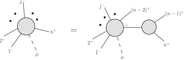
Figure 3: Diagram corresponding to the recursion relation (81) for $A_{n}^{(0)}(\phi,1^{-},2^{+},\dots,j^{-},\dots,n^{+})$.

Another infinite series of tree-level $\phi$ amplitudes is the “maximally googly” set BGK ,

$$A_{n}^{(0)}(\phi,1^{-},2^{-},3^{-},\dots,n^{-}) = i{(-1)^{n}(k_{\phi}^{2})^{2}\over\left[1\,2\right]\left[2\,3\right]\cdots\left[n\,1\right]}\,,$$ (84)

$$A_{n}^{(0)}(\phi^{\dagger},1^{+},2^{+},3^{+},\dots,n^{+}) = i{(k_{\phi}^{2})^{2}\over\left\langle 1\,2\right\rangle\left\langle 2\,3\right\rangle\cdots\left\langle n\,1\right\rangle}\,.$$ (85)

IV.3 Coupling of $A$ to the axial current divergence, and the $\phi g^{+}g^{+}$ amplitude

As mentioned in section II.1, at order $\alpha_{s}^{2}$ in the effective theory, the pseudoscalar $A$ begins to couple to the divergence of the light-quark axial current CKSB . The full effective Lagrangian is given by

$$\mathcal{L}_{A}^{\mbox{\tiny int}}=\frac{C}{2}A\,\mathop{\rm tr}\nolimits G_{\mu\nu}\mbox{ }^{*}G^{\mu\nu}+\frac{C^{\prime}}{2}A\,\partial_{\mu}\sum\limits_{i=1}^{n_{l}}\bar{q}_{i}\gamma^{\mu}\gamma_{5}q_{i}\,,$$ (86)

where the sum is over all light quark flavors $n_{l}$, and $C$ and $C^{\prime}$ denote the appropriate coefficients, which begin at order $\alpha_{s}$ for $C$ and order $\alpha_{s}^{2}$ for $C^{\prime}$. It was found in ref. CKSB by explicit calculation that the second term in eq. (86) does not contribute at NLO, in accordance with a non-Abelian version NAABth of the Adler-Bardeen theorem ABth . This can also be seen via recursion relations as follows: The amplitude $A_{2}^{{(0)}}(A_{J_{5}},1_{f}^{-},2_{f}^{+})$ vanishes by helicity conservation for massless fermions $f$. We have denoted the contribution from the second term in eq. (86) by the subscript $J_{5}$. By $A_{2}^{{(0)}}$ we mean a tree amplitude, which contributes at NLO due to the factor of $\alpha_{s}^{2}$ in $C^{\prime}$. The effective $A\bar{q}q$-vertex is proportional to the momentum that flows through it due to the derivative in eq. (86). When attaching a gluon to this vertex, one can choose its polarization vector so that each of the two diagrams contributing to $A_{3}^{{(0)}}(A_{J_{5}},1_{f}^{-},2_{f}^{+},3^{\pm})$ vanishes. (The amplitude is of course gauge invariant; in other gauges the two diagrams cancel against each other.) Thus $A_{3}^{{(0)}}(A_{J_{5}},1_{f}^{-},2_{f}^{+},3^{\pm})=0$. By recursion, the amplitudes with an arbitrary number of gluons also vanish — there are no lower-point amplitudes to contribute to the right-hand side of a recursion relation. Thus we do not need to consider the contribution of the light-quark axial current at NLO, and the amplitudes involving a pseudoscalar $A$ can be constructed via eq. (7).

In appendix A we compute the simplest, finite one-loop amplitude with a single $\phi$ field, $A_{2;1}(\phi,1^{+},2^{+})$. The result can be written in terms of the “googly” two-gluon tree amplitude,

$$A_{2;1}(\phi,1^{+},2^{+})=-2A_{2}^{(0)}(\phi^{\dagger},1^{+},2^{+})\,.$$ (87)

This amplitude enters recursively into all the subsequently constructed amplitudes.

V The soft Higgs limit

It is useful to consider the kinematic limit of the single-$\phi$ amplitudes as $k_{\phi}\to 0$. Of course this soft-Higgs limit can only be reached if $m_{H}=0$. The limiting behavior of single-$\phi$ tree amplitudes was studied in ref. DGK . Here we review that analysis and extend it to the loop level. First consider amplitudes with a single real scalar field $H$, as the Higgs momentum goes to zero, so that $H$ has almost no spatial variation. Then the $H\mathop{\rm tr}\nolimits G_{\mu\nu}G^{\mu\nu}$ interaction behaves just like a constant multiple of the pure-glue Lagrangian $\mathop{\rm tr}\nolimits G_{\mu\nu}G^{\mu\nu}$. So one might expect the Higgs-plus-$n$-gluon amplitudes to become proportional to the pure-gauge-theory amplitudes, according to the relation,

$${\cal A}_{n}(H,\{k_{i},\lambda_{i},a_{i}\})\longrightarrow({\rm const.})\times{\partial\over\partial g}{\cal A}_{n}(\{k_{i},\lambda_{i},a_{i}\})\qquad\quad\hbox{as $k_{H}\to 0$,}$$ (88)

for any helicity configuration. Taking into account the number of factors of the gauge coupling in the $n$-parton tree amplitudes, namely $(n-2)$, eq. (88) leads to the tree-level soft Higgs limit,

$$A_{n}^{{(0)}}(H,1,2,3,\ldots,n)\longrightarrow(n-2)A_{n}^{{(0)}}(1,2,3,\ldots,n)\qquad\quad\hbox{as $k_{H}\to 0$,}$$ (89)

which holds color structure by color structure. Similarly, at $l$ loops, our naive expectation for the soft limit is,

$$A_{n}^{{(l)}}(H,1,2,3,\ldots,n)\longrightarrow(n+2\,l-2)A_{n}^{{(l)}}(1,2,3,\ldots,n)\qquad\quad\hbox{as $k_{H}\to 0$.}$$ (90)

In fact, we will find that eq. (90) is not precisely correct beyond tree level. A generalization of this equation to the case of $\phi$ and $\phi^{\dagger}$ amplitudes will hold at loop level, but again it will hold precisely only for the finite one-loop amplitudes. Equation (90) generically breaks down at loop level because of an exchange-of-limits problem, between dimensional regularization of infrared divergences, and the momentum injected into the amplitude by the Higgs boson, which acts as a kind of effective infrared regulator as well.

Before examining the infrared issue, let us first propose an extension of eq. (90) to the case of amplitudes with a single $\phi$, or $\phi^{\dagger}$. At tree level, by studying the MHV representation of the $\phi$ and $\phi^{\dagger}$ amplitudes, it can be shown DGK that the factor of $(n-2)$ in eq. (89) is partitioned into $(n_{-}-1)$ and $(n_{+}-1)$ in the two cases,

$$A_{n}^{(0)}(\phi,1,2,3,\ldots,n)\longrightarrow(n_{-}-1)A_{n}^{(0)}(1,2,3,\ldots,n)\qquad\quad\hbox{as $k_{\phi}\to 0$,}$$ (91)

and (by parity)

$$A_{n}^{(0)}(\phi^{\dagger},1,2,3,\ldots,n)\longrightarrow(n_{+}-1)A_{n}^{(0)}(1,2,3,\ldots,n)\qquad\quad\hbox{as $k_{\phi}\to 0$,}$$ (92)

where $n_{\pm}$ are the number of external partons with helicity $\pm 1$ for gluons ($\pm{1\over 2}$ for fermions). The natural generalization of eqs. (91) and (92) to $l$ loops would be,

$$A_{n}^{(l)}(\phi,1,2,3,\ldots,n)\longrightarrow(n_{-}+l-1)A_{n}^{(l)}(1,2,3,\ldots,n)\qquad\quad\hbox{as $k_{\phi}\to 0$,}$$ (93)

and

$$A_{n}^{(l)}(\phi^{\dagger},1,2,3,\ldots,n)\longrightarrow(n_{+}+l-1)A_{n}^{(l)}(1,2,3,\ldots,n)\qquad\quad\hbox{as $k_{\phi}\to 0$.}$$ (94)

But again, infrared complications can affect these relations.

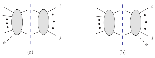
Figure 4: Two cuts of a one-loop $\phi$ amplitude which become the same cut in the soft limit $k_{\phi}\to 0$: (a) the cut in the $s_{i\cdots j}$ channel, and (b) the cut in the $s_{\phi,i\cdots j}$ channel.

Consider a particular class of terms in a one-loop Higgs or $\phi$ amplitude, those containing a cut in either the $s_{i\cdots j}$ channel or the $s_{\phi,i\cdots j}$ channel, as illustrated in fig. 4. The soft behavior of these terms can be analyzed using unitarity, plus the tree-level soft behavior. The two cuts in fig. 4 become identical, up to constant factors, as $k_{\phi}\to 0$. Suppose there are $m$ external partons on the right side of the cuts in fig. 4, plus the two crossing the cut. Then there are $(n-m)$ external partons on the left side of the cut, plus two more crossing the cut. (The fields $H$ and $\phi$ do not count as partons.) For the case of a Higgs field $H$, using eq. (89) in the soft limit $k_{H}\to 0$, the cut in fig. 4(a) reduces to the pure-QCD cut in the $s_{i\cdots j}$ channel, multiplied by a factor of $(n-m)$. The cut in fig. 4(b) reduces to the same pure-QCD cut, because $s_{\phi,i\cdots j}\to s_{i\cdots j}$, but it is multiplied by a factor of $m$. Summing the two contributions, we find that the terms in the loop amplitude containing $\ln(-s_{i\cdots j})$ and $\ln(-s_{\phi,i\cdots j})$ go smoothly into the terms containing $\ln(-s_{i\cdots j})$ in the pure-QCD amplitude, multiplied by a factor of $(n-m)+m=n$. This argument would seem to prove eq. (90) for $l=1$.

A similar argument applies to the $\phi$ and $\phi^{\dagger}$ amplitudes. If there are a total of $n_{\pm,L}$ partons with helicity $\pm 1$ on the left-hand side of the cut, and $n_{\pm,R}$ on the right-hand side, then $n_{\pm,L}+n_{\pm,R}=n_{\pm}+2$, because 2 partons of each helicity are assigned to the cut. Instead of the multiplicative factor of $(n-m)+m=n$ found for the case of $H$, for $\phi$ we get from eq. (91) a factor of $(n_{-,L}-1)+(n_{-,R}-1)=n_{-}$, which is the factor in eq. (93) for $l=1$.

However, both these arguments break down for the case $m=2$, for which only two partons, $i$ and $i+1$, appear on the right-hand side of the cut. In this case, the cut in fig. 4(a) is generically infrared divergent, whereas the cut in fig. 4(b) is infrared finite, for nonzero momentum $k_{\phi}$. The generic form of one-loop divergences for the unrenormalized amplitudes for an $H$ or $\phi$ field plus $n$ gluons, for example, is UniversalIR

$$A_{n;1}(H,1,2,\ldots,n) = -{1\over\epsilon^{2}}\sum_{i=1}^{n}\left({\mu^{2}\over-s_{i,i+1}}\right)^{\epsilon}A_{n}^{(0)}(H,1,2,\ldots,n)\ +\ \hbox{finite,}$$ (95)

$$A_{n;1}(\phi,1,2,\ldots,n) = -{1\over\epsilon^{2}}\sum_{i=1}^{n}\left({\mu^{2}\over-s_{i,i+1}}\right)^{\epsilon}A_{n}^{(0)}(\phi,1,2,\ldots,n)\ +\ \hbox{finite.}$$ (96)

The infrared divergences have precisely the same form as for pure QCD,

$$A_{n;1}(1,2,\ldots,n)=\Biggl{[}-{1\over\epsilon^{2}}\sum_{i=1}^{n}\left({\mu^{2}\over-s_{i,i+1}}\right)^{\epsilon}-{\beta_{0}\over\epsilon}\Biggr{]}A_{n}^{(0)}(1,2,\ldots,n)\ +\ \hbox{finite,}$$ (97)

where $\beta_{0}=(11N_{c}-2n_{\!f}-n_{s})/(3N_{c})$. (After ultraviolet renormalization the remaining infrared $\beta_{0}$ terms match between eqs. (95)–(97).) Hence the divergent parts of the (renormalized) one-loop $H$ and $\phi$ amplitudes have the soft behavior characteristic of the tree-level amplitudes,

$$A_{n;1}(H,1,2,\ldots,n)\Big{|}_{1/\epsilon\ {\rm poles}} \buildrel k_{H}\to 0\over{\relbar\mskip-0.5mu\joinrel\mskip-0.5mu\relbar\mskip-0.5mu\joinrel\longrightarrow} (n-2)\,A_{n;1}(1,2,\ldots,n)\Big{|}_{1/\epsilon\ {\rm poles}}\ ,$$ (98)

$$A_{n;1}(\phi,1,2,\ldots,n)\Big{|}_{1/\epsilon\ {\rm poles}} \buildrel k_{\phi}\to 0\over{\relbar\mskip-0.5mu\joinrel\mskip-0.5mu\relbar\mskip-0.5mu\joinrel\longrightarrow} (n_{-}-1)\,A_{n;1}(1,2,\ldots,n)\Big{|}_{1/\epsilon\ {\rm poles}}\ .$$ (99)

This behavior does not agree with the naive expectation for the one-loop behavior, eqs. (90) and (93) for $l=1$. However, it is consistent with the behavior of the divergent cuts for $j=i+1$ ($m=2$) in fig. 4. For example the factor of $(n-2)$ in eq. (98), for the cut of the term proportional to $\ln(-s_{i,i+1})/\epsilon\times A_{n}^{(0)}$, comes just from fig. 4(a), because the cut of fig. 4(b) has no pole in $\epsilon$. It is the exchange of limits, $\epsilon\to 0$ and $k_{H}\to 0$, in fig. 4(b), which is at the root of the non-uniform soft behavior.

This argument does not cover the cases $m=1$ ($\ln(-s_{\phi,i})$ terms) or $m=0$ ($\ln(-k_{\phi}^{2})$ terms). These cases have only the cuts shown in fig. 4(b), but the cuts become quite singular in the $k_{\phi}\to 0$ limit, so we may expect non-uniform soft behavior. The cut-based argument also does not tell us what to expect for the rational terms in generic $H$ or $\phi$ amplitudes. Indeed, for the one-loop $H\bar{q}q\bar{Q}\bar{Q}$ amplitudes presented in ref. EGZHiggs , the soft Higgs limits of the generic cut terms (all of which have $m=0$, 1, or 2) and rational parts at order $\epsilon^{0}$ do not appear to be uniform.

On the other hand, for the finite $\phi$ amplitudes we focus on in this paper, there should be no infrared issues, and hence we should find the simple, uniform behavior, valid for each color structure,

$$A_{n}^{(1)}(\phi,1,2,3,\ldots,n)\buildrel k_{\phi}\to 0\over{\relbar\mskip-0.5mu\joinrel\mskip-0.5mu\relbar\mskip-0.5mu\joinrel\longrightarrow}n_{-}\,A_{n}^{(1)}(1,2,3,\ldots,n)\qquad\quad\hbox{(finite helicity configurations).}$$ (100)

We shall verify eq. (100) explicitly below for the finite helicity amplitudes.

Assuming that eq. (100) holds, then the generic one-loop amplitude with $\phi$ present must be at least as complicated as the corresponding pure-QCD amplitude with $\phi$ omitted, because the former amplitude must reduce to the latter amplitude, multiplied by a factor of $n_{-}$, as $k_{\phi}\to 0$. The one possible exception is the all-plus amplitude, $A_{n}^{(1)}(\phi,1^{+},2^{+},\ldots,n^{+})$, because the multiplicative factor vanishes in this case. Indeed, as we shall see in the next section, these amplitudes are given by a much simpler formula than the corresponding QCD result (61).

VI Recursion relation for all-plus case

Using the results of section III, and the explicit calculation of the two-gluon one-loop amplitude (87), we can recursively construct the following form of the one-loop all-plus $\phi$ amplitude,

$$A_{n}^{[f]}(\phi,1^{+},2^{+},\dots,n^{+}) = A_{n}^{[s]}(\phi,1^{+},2^{+},\dots,n^{+})=0\,,$$ (101)

$$A_{n}^{[g]}(\phi,1^{+},2^{+},\dots,n^{+}) = -2i{(k_{\phi}^{2})^{2}\over\left\langle 1\,2\right\rangle\left\langle 2\,3\right\rangle\cdots\left\langle n\,1\right\rangle}=-2A_{n}^{(0)}(\phi^{\dagger},1^{+},2^{+},\dots,n^{+})\,.$$ (102)

The proof of eq. (102) is analogous to the above proof of the tree-level MHV amplitude via an on-shell recursion relation BCFRecursion .

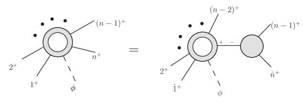
Figure 5: Diagram corresponding to the recursion relation (103) for $A_{n}^{(1)}(\phi,1^{+},2^{+},\ldots,n^{+})$.

Here we use again the $[1,n\rangle$ shift (80). As in section IV.2 there is only one term contributing to the recursion, as illustrated in fig. 5,

$$A_{n;1}(\phi,1^{+},\dots,n^{+})$$

$$\hskip 8.5359pt=A_{n-1;1}(\phi,\hat{1}^{+},2^{+},\dots,(n-2)^{+},\hat{K}_{n-1,n}^{+})\,\frac{i}{s_{n-1,n}}\,A_{3}^{(0)}((n-1)^{+},\hat{n}^{+},-\hat{K}_{n-1,n}^{-})\,.~{}~{}~{}~{}$$ (103)

It is straightforward to show that eq. (102) satisfies eq. (103), using the same algebra as in eq. (82). The amplitude $A_{n}^{[g]}(\phi,1^{+},2^{+},\dots,n^{+})$ in eq. (102) vanishes in the soft limit, just as predicted by eq. (100) for $n_{-}=0$.

Note that the lack of $n_{\!f}$ or $n_{s}$ dependence in $A_{2;1}(\phi,1^{+},2^{+})$ translates recursively into the vanishing of $A_{n}^{[f]}$ and $A_{n}^{[s]}$ in eq. (101), for all values of $n$. Now consider the dependence of the one-loop one-minus $\phi$ amplitude on $n_{\!f}$ or $n_{s}$. This amplitude factorizes onto two types of one-loop amplitudes, either the all-plus $\phi$ amplitude, which obeys eq. (101), or the all-plus pure-QCD amplitude. But the pure-QCD amplitude obeys $A_{n}^{[f]}=-A_{n}^{[s]}$, thanks to a supersymmetric Ward identity SWI . Using this relation and eq. (101) in a recursive argument, we must have $A_{n}^{[f]}=-A_{n}^{[s]}$ also for the one-minus $\phi$ amplitude, as mentioned in section II, and as assumed in the color decomposition (18).

VII Quark recursion relations

As we discussed in section II, for the finite helicity amplitudes — one quark pair, with all gluons having positive helicity — there are two independent primitive amplitudes that need to be computed,

$$A_{n}^{L-s}(\phi,j_{\!f}^{+}) \equiv A_{n}^{L-s}(\phi,1_{\!f}^{-},2^{+},\ldots,j_{\!f}^{+},\ldots,n^{+})\,,\qquad 2\leq j\leq n,$$ (104)

$$A_{n}^{s}(\phi,j_{\!f}^{+}) \equiv A_{n}^{s}(\phi,1_{\!f}^{-},2^{+},\ldots,j_{\!f}^{+},\ldots,n^{+})\,,\qquad 2\leq j\leq n-2\,.$$ (105)

We abbreviate the notation as in ref. LastFinite , retaining only the label of the positive-helicity fermion (and $\phi$). A computation of these primitive amplitudes determines all the finite one-loop quark amplitudes for a single $\phi$ boson coupled to QCD.

VII.1 Recursion relation for $L-s$ contribution

As mentioned in the introduction and in section III, finite quark-gluon amplitudes in both pure QCD and $\phi$-amplitudes contain “unreal” poles. The contributions of the unreal poles can be described using a “soft factor” ${\cal S}^{(0)}$ reminiscent of the propagation of an internal soft gluon LastFinite .

For the recursive construction we need the “$L\!-\!s$ loop vertex” introduced in ref. LastFinite ,

$$V_{3}^{L-s}(1^{+},2^{+},3^{+})\equiv-{i\over 2}\left[1\,2\right]\left[2\,3\right]\left[3\,1\right]\,.$$ (106)

The soft factor ${\cal S}^{(0)}(a,s,b)$ traditionally describes the insertion of a soft gluon $s$ between two hard partons $a$ and $b$ in a color-ordered amplitude. It depends only on the helicity of the soft gluon and is given by TreeReview ,

$${\cal S}^{(0)}(a,s^{+},b) = {\left\langle a\,b\right\rangle\over\left\langle a\,s\right\rangle\left\langle s\,b\right\rangle}\,,$$ (107)

$${\cal S}^{(0)}(a,s^{-},b) = -{\left[a\,b\right]\over\left[a\,s\right]\left[s\,b\right]}\,.$$ (108)

Choosing the shifted legs in eq. (39) to be $[k,l\rangle=[1,n\rangle$, eq. (80), the recursion relation for the pure-QCD amplitude $A_{n}^{L-s}(j_{\!f}^{+})\equiv A_{n}^{L-s}(1_{\!f}^{-},2^{+},\ldots,j_{\!f}^{+},\ldots,n^{+})$ was found to be,

$$\hbox{}\hskip-28.45274ptA_{n}^{L-s}(j_{\!f}^{+})$$ (109)

$$= A_{n-1}^{L-s}(\hat{1}_{\!f}^{-},2^{+},\ldots,j_{\!f}^{+},\ldots,(n-2)^{+},{\hat{K}}_{n-1,n}^{+})\,{i\over s_{n-1,n}}\,A_{3}^{{(0)}}(-{\hat{K}}_{n-1,n}^{-},(n-1)^{+},\hat{n}^{+})$$

$$\hskip-11.38109pt\hbox{}+A_{n-1}^{(0)}(\hat{1}_{\!f}^{-},2^{+},\ldots,j_{\!f}^{+},\ldots,(n-2)^{+},{\hat{K}}_{n-1,n}^{-})\,{i\over s_{n-1,n}}\,V_{3}^{L-s}(-{\hat{K}}_{n-1,n}^{+},(n-1)^{+},\hat{n}^{+})$$

$$\hskip 56.9055pt\hbox{}\times{\cal S}^{(0)}(j,{\hat{K}}_{n-1,n}^{+},\hat{1})\,{\cal S}^{(0)}(\hat{n},-{\hat{K}}_{n-1,n}^{-},n-1)\,,$$

where the hatted momenta in eq. (109) are defined by the shift (80), with

$$z=-{K_{n-1,n}^{2}\over\left\langle\smash{1}{\vphantom{1}}^{-}\right|{{\raise 0.91666pt\hbox to9.20833pt{\hss/\hss}\hbox to0.0pt{\hss$K$}}_{n-1,n}}\left|\smash{n}{\vphantom{1}}^{-}\right\rangle}=-{\left\langle(n-1)\,n\right\rangle\over\left\langle(n-1)\,1\right\rangle}\,,$$ (110)

in each term. The second term in eq. (109) represents the contribution of an unreal pole. The solution to eq. (109) is given by eq. (71).

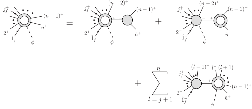
Figure 6: Diagrams corresponding to the terms in the recursion relation (111) for $A_{n}^{L-s}(\phi,j_{\!f}^{+})$, for $j\leq n-2$. The second term contains an unreal pole. In the last term, the sum over $l$ runs from $j+1$ to $n$, inclusive.

For the analogous single-$\phi$ amplitude $A_{n}^{L-s}(\phi,j_{\!f}^{+})$, using the same $[1,n\rangle$ shift, the $n$-point on-shell recursion relation is, for $j\leq n-2$,

$$\hbox{}\hskip-28.45274ptA_{n}^{L-s}(\phi,j_{\!f}^{+})$$

$$= A_{n-1}^{L-s}(\phi,\hat{1}_{\!f}^{-},2^{+},\ldots,j_{\!f}^{+},\ldots,(n-2)^{+},{\hat{K}}_{n-1,n}^{+})\,{i\over s_{n-1,n}}\,A_{3}^{{(0)}}(-{\hat{K}}_{n-1,n}^{-},(n-1)^{+},\hat{n}^{+})$$

$$\hskip-11.38109pt\hbox{}+A_{n-1}^{(0)}(\phi,\hat{1}_{\!f}^{-},2^{+},\ldots,j_{\!f}^{+},\ldots,(n-2)^{+},{\hat{K}}_{n-1,n}^{-})\,{i\over s_{n-1,n}}\,V_{3}^{L-s}(-{\hat{K}}_{n-1,n}^{+},(n-1)^{+},\hat{n}^{+})$$

$$\hskip 56.9055pt\hbox{}\times{\cal S}^{(0)}(j,{\hat{K}}_{n-1,n}^{+},\hat{1})\,{\cal S}^{(0)}(\hat{n},-{\hat{K}}_{n-1,n}^{-},n-1)$$

$$\hskip-11.38109pt\hbox{}+\sum_{l=j+1}^{n}A_{l}^{(0)}(\hat{1}_{\!f}^{-},2^{+},\ldots,j_{\!f}^{+},\ldots,(l-1)^{+},{\hat{K}}_{\phi,l\cdots n}^{-})\,{i\over s_{\phi,l\cdots n}}\,A_{n-l+2}^{[g]}(\phi,-{\hat{K}}_{\phi,l\cdots n}^{+},l^{+},\ldots,\hat{n}^{+})\,,$$

(111)

where in the $s_{\phi,l\cdots n}$ channel we set,

$$z=-{s_{\phi,l\cdots n}\over\left\langle\smash{1}{\vphantom{1}}^{-}\right|{{\raise 0.91666pt\hbox to9.20833pt{\hss/\hss}\hbox to0.0pt{\hss$K$}}_{\phi,l\cdots n}}\left|\smash{n}{\vphantom{1}}^{-}\right\rangle}={s_{1\cdots(l-1)}\over\left\langle\smash{1}{\vphantom{1}}^{-}\right|{{\raise 0.91666pt\hbox to9.20833pt{\hss/\hss}\hbox to0.0pt{\hss$K$}}_{1\cdots(l-1)}}\left|\smash{n}{\vphantom{1}}^{-}\right\rangle}\,.$$ (112)

The recursion relation is shown in fig. 6. Again the second term represents the unreal-pole contribution, which we take to have the same form when $\phi$ is present as it does in pure QCD. The additional third term in eq. (111), containing a sum over $l$, arises because the amplitudes $A_{m}^{[g]}(\phi,+,+,\ldots,+)=A_{m}^{[g-s]}(\phi,+,+,\ldots,+)$ are nonvanishing when $\phi$ is present. The corresponding pure-QCD amplitude combination $A_{m}^{[g-s]}(+,+,\ldots,+)$ vanishes according to eq. (61), so there is no such term in the pure-QCD recursion relation (109).

The solution to eq. (111) is,

$$A_{n}^{L-s}(\phi,1_{\!f}^{-},2^{+},\ldots,j_{\!f}^{+},\ldots,n^{+})={i\over 2}{Q_{0}^{\phi}+Q_{1}^{\phi}+Q_{2}^{\phi}\over\left\langle 1\,2\right\rangle\left\langle 2\,3\right\rangle\cdots\left\langle n\,1\right\rangle}\,,$$ (113)

where

$$Q_{0}^{\phi} = \left\langle 1\,j\right\rangle\sum_{l=2}^{n-1}\left\langle\smash{1}{\vphantom{1}}^{-}\right|{{\raise 0.97221pt\hbox to5.52084pt{\hss/\hss}\hbox to0.0pt{\hss$k$}}_{l}{\raise 0.91666pt\hbox to9.20833pt{\hss/\hss}\hbox to0.0pt{\hss$K$}}_{l\cdots n}}\left|\smash{1}{\vphantom{1}}^{+}\right\rangle\,,$$ (114)

$$Q_{1}^{\phi} = -4\sum_{l=j+1}^{n}{\left\langle(l-1)\,l\right\rangle\over\left\langle\smash{1}{\vphantom{1}}^{-}\right|{{\raise 0.91666pt\hbox to9.20833pt{\hss/\hss}\hbox to0.0pt{\hss$K$}}_{l\cdots n}{\raise 0.91666pt\hbox to9.20833pt{\hss/\hss}\hbox to0.0pt{\hss$K$}}_{1\cdots n}}\left|\smash{(l-1)}{\vphantom{1}}^{+}\right\rangle\left\langle\smash{1}{\vphantom{1}}^{-}\right|{{\raise 0.91666pt\hbox to9.20833pt{\hss/\hss}\hbox to0.0pt{\hss$K$}}_{2\cdots(l-1)}{\raise 0.91666pt\hbox to9.20833pt{\hss/\hss}\hbox to0.0pt{\hss$K$}}_{1\cdots n}}\left|\smash{l}{\vphantom{1}}^{+}\right\rangle}$$ (115)

$$\hskip 28.45274pt\hbox{}\times{\left\langle\smash{1}{\vphantom{1}}^{-}\right|{{\raise 0.91666pt\hbox to9.20833pt{\hss/\hss}\hbox to0.0pt{\hss$K$}}_{2\cdots(l-1)}{\raise 0.91666pt\hbox to9.20833pt{\hss/\hss}\hbox to0.0pt{\hss$K$}}_{l\cdots n}}\left|\smash{1}{\vphantom{1}}^{+}\right\rangle}^{2}\left\langle\smash{j}{\vphantom{1}}^{-}\right|{{\raise 0.91666pt\hbox to9.20833pt{\hss/\hss}\hbox to0.0pt{\hss$K$}}_{1\cdots n}{\raise 0.91666pt\hbox to9.20833pt{\hss/\hss}\hbox to0.0pt{\hss$K$}}_{l\cdots n}}\left|\smash{1}{\vphantom{1}}^{+}\right\rangle\,,$$

$$Q_{2}^{\phi} = -4\sum_{l=j+1}^{n-1}\sum_{p=l+1}^{n}{\left\langle(l-1)\,l\right\rangle\over\left\langle\smash{1}{\vphantom{1}}^{-}\right|{{\raise 0.91666pt\hbox to9.20833pt{\hss/\hss}\hbox to0.0pt{\hss$K$}}_{p\cdots n}({\raise 0.91666pt\hbox to9.20833pt{\hss/\hss}\hbox to0.0pt{\hss$K$}}_{1\cdots(l-1)}+{\raise 0.91666pt\hbox to9.20833pt{\hss/\hss}\hbox to0.0pt{\hss$K$}}_{p\cdots n})}\left|\smash{(l-1)}{\vphantom{1}}^{+}\right\rangle\left\langle\smash{1}{\vphantom{1}}^{-}\right|{{\raise 0.91666pt\hbox to9.20833pt{\hss/\hss}\hbox to0.0pt{\hss$K$}}_{p\cdots n}({\raise 0.91666pt\hbox to9.20833pt{\hss/\hss}\hbox to0.0pt{\hss$K$}}_{1\cdots(l-1)}+{\raise 0.91666pt\hbox to9.20833pt{\hss/\hss}\hbox to0.0pt{\hss$K$}}_{p\cdots n})}\left|\smash{l}{\vphantom{1}}^{+}\right\rangle}$$ (116)

$$\hskip 17.07164pt\hbox{}\times{\left\langle(p-1)\,p\right\rangle\over\left\langle\smash{1}{\vphantom{1}}^{-}\right|{{\raise 0.91666pt\hbox to9.20833pt{\hss/\hss}\hbox to0.0pt{\hss$K$}}_{2\cdots(l-1)}({\raise 0.91666pt\hbox to9.20833pt{\hss/\hss}\hbox to0.0pt{\hss$K$}}_{1\cdots(l-1)}+{\raise 0.91666pt\hbox to9.20833pt{\hss/\hss}\hbox to0.0pt{\hss$K$}}_{p\cdots n})}\left|\smash{(p-1)}{\vphantom{1}}^{+}\right\rangle\left\langle\smash{1}{\vphantom{1}}^{-}\right|{{\raise 0.91666pt\hbox to9.20833pt{\hss/\hss}\hbox to0.0pt{\hss$K$}}_{2\cdots(l-1)}({\raise 0.91666pt\hbox to9.20833pt{\hss/\hss}\hbox to0.0pt{\hss$K$}}_{1\cdots(l-1)}+{\raise 0.91666pt\hbox to9.20833pt{\hss/\hss}\hbox to0.0pt{\hss$K$}}_{p\cdots n})}\left|\smash{p}{\vphantom{1}}^{+}\right\rangle}$$

$$\hskip 17.07164pt\hbox{}\times{\left\langle\smash{1}{\vphantom{1}}^{-}\right|{{\raise 0.91666pt\hbox to9.20833pt{\hss/\hss}\hbox to0.0pt{\hss$K$}}_{2\cdots(l-1)}{\raise 0.91666pt\hbox to9.20833pt{\hss/\hss}\hbox to0.0pt{\hss$K$}}_{p\cdots n}}\left|\smash{1}{\vphantom{1}}^{+}\right\rangle}^{3}\left\langle\smash{j}{\vphantom{1}}^{-}\right|{({\raise 0.91666pt\hbox to9.20833pt{\hss/\hss}\hbox to0.0pt{\hss$K$}}_{1\cdots(l-1)}+{\raise 0.91666pt\hbox to9.20833pt{\hss/\hss}\hbox to0.0pt{\hss$K$}}_{p\cdots n}){\raise 0.91666pt\hbox to9.20833pt{\hss/\hss}\hbox to0.0pt{\hss$K$}}_{p\cdots n}}\left|\smash{1}{\vphantom{1}}^{+}\right\rangle$$

$$\hskip 17.07164pt\hbox{}\times{(k_{\phi}^{2})^{2}\over(K_{1\cdots(l-1)}+K_{p\cdots n})^{2}}\,.$$

Making use of momentum conservation, eq. (29), antisymmetry of the spinor products, and re-indexing the sum over $p$ in $Q_{2}^{\phi}$, we can rewrite these quantities as

$$Q_{0}^{\phi} = \left\langle 1\,j\right\rangle\sum_{l=2}^{n-1}\left\langle\smash{1}{\vphantom{1}}^{-}\right|{{\raise 0.91666pt\hbox to9.20833pt{\hss/\hss}\hbox to0.0pt{\hss$K$}}_{\phi,2\cdots l}{\raise 0.97221pt\hbox to5.52084pt{\hss/\hss}\hbox to0.0pt{\hss$k$}}_{l}}\left|\smash{1}{\vphantom{1}}^{+}\right\rangle\,,$$ (117)

$$Q_{1}^{\phi} = -4\sum_{l=j+1}^{n}{\left\langle(l-1)\,l\right\rangle\over\left\langle\smash{1}{\vphantom{1}}^{-}\right|{{\raise 0.91666pt\hbox to9.20833pt{\hss/\hss}\hbox to0.0pt{\hss$K$}}_{l\cdots n}{\raise 0.97221pt\hbox to5.52084pt{\hss/\hss}\hbox to0.0pt{\hss$k$}}_{\phi}}\left|\smash{(l-1)}{\vphantom{1}}^{+}\right\rangle\left\langle\smash{1}{\vphantom{1}}^{-}\right|{{\raise 0.91666pt\hbox to9.20833pt{\hss/\hss}\hbox to0.0pt{\hss$K$}}_{2\cdots(l-1)}{\raise 0.97221pt\hbox to5.52084pt{\hss/\hss}\hbox to0.0pt{\hss$k$}}_{\phi}}\left|\smash{l}{\vphantom{1}}^{+}\right\rangle}$$ (118)

$$\hskip 28.45274pt\hbox{}\times{\left\langle\smash{1}{\vphantom{1}}^{-}\right|{{\raise 0.91666pt\hbox to9.20833pt{\hss/\hss}\hbox to0.0pt{\hss$K$}}_{l\cdots n}{\raise 0.97221pt\hbox to5.52084pt{\hss/\hss}\hbox to0.0pt{\hss$k$}}_{\phi}}\left|\smash{1}{\vphantom{1}}^{+}\right\rangle}^{2}\left\langle\smash{1}{\vphantom{1}}^{-}\right|{{\raise 0.91666pt\hbox to9.20833pt{\hss/\hss}\hbox to0.0pt{\hss$K$}}_{l\cdots n}{\raise 0.97221pt\hbox to5.52084pt{\hss/\hss}\hbox to0.0pt{\hss$k$}}_{\phi}}\left|\smash{j}{\vphantom{1}}^{+}\right\rangle\,,$$

$$Q_{2}^{\phi} = -4\sum_{l=j+1}^{n-1}\sum_{p=l}^{n-1}{\left\langle(l-1)\,l\right\rangle\over\left\langle\smash{1}{\vphantom{1}}^{-}\right|{{\raise 0.91666pt\hbox to9.20833pt{\hss/\hss}\hbox to0.0pt{\hss$K$}}_{(p+1)\cdots n}{\raise 0.91666pt\hbox to9.20833pt{\hss/\hss}\hbox to0.0pt{\hss$K$}}_{\phi,l\cdots p}}\left|\smash{(l-1)}{\vphantom{1}}^{+}\right\rangle\left\langle\smash{1}{\vphantom{1}}^{-}\right|{{\raise 0.91666pt\hbox to9.20833pt{\hss/\hss}\hbox to0.0pt{\hss$K$}}_{(p+1)\cdots n}{\raise 0.91666pt\hbox to9.20833pt{\hss/\hss}\hbox to0.0pt{\hss$K$}}_{\phi,l\cdots p}}\left|\smash{l}{\vphantom{1}}^{+}\right\rangle}$$ (119)

$$\hskip 17.07164pt\hbox{}\times{\left\langle p\,(p+1)\right\rangle\over\left\langle\smash{1}{\vphantom{1}}^{-}\right|{{\raise 0.91666pt\hbox to9.20833pt{\hss/\hss}\hbox to0.0pt{\hss$K$}}_{2\cdots(l-1)}{\raise 0.91666pt\hbox to9.20833pt{\hss/\hss}\hbox to0.0pt{\hss$K$}}_{\phi,l\cdots p}}\left|\smash{p}{\vphantom{1}}^{+}\right\rangle\left\langle\smash{1}{\vphantom{1}}^{-}\right|{{\raise 0.91666pt\hbox to9.20833pt{\hss/\hss}\hbox to0.0pt{\hss$K$}}_{2\cdots(l-1)}{\raise 0.91666pt\hbox to9.20833pt{\hss/\hss}\hbox to0.0pt{\hss$K$}}_{\phi,l\cdots p}}\left|\smash{(p+1)}{\vphantom{1}}^{+}\right\rangle}$$

$$\hskip 17.07164pt\hbox{}\times{\left\langle\smash{1}{\vphantom{1}}^{-}\right|{{\raise 0.91666pt\hbox to9.20833pt{\hss/\hss}\hbox to0.0pt{\hss$K$}}_{(p+1)\cdots n}{\raise 0.91666pt\hbox to9.20833pt{\hss/\hss}\hbox to0.0pt{\hss$K$}}_{\phi,l\cdots p}}\left|\smash{1}{\vphantom{1}}^{+}\right\rangle}^{3}\left\langle\smash{1}{\vphantom{1}}^{-}\right|{{\raise 0.91666pt\hbox to9.20833pt{\hss/\hss}\hbox to0.0pt{\hss$K$}}_{(p+1)\cdots n}{\raise 0.91666pt\hbox to9.20833pt{\hss/\hss}\hbox to0.0pt{\hss$K$}}_{\phi,l\cdots p}}\left|\smash{j}{\vphantom{1}}^{+}\right\rangle\ {(k_{\phi}^{2})^{2}\over s_{\phi,l\cdots p}}\,.$$

The latter forms make the soft-$\phi$ limit, $k_{\phi}\to 0$, somewhat more manifest. In this limit, we see that $Q_{0}^{\phi}$ reduces to $Q_{0}$ as given in eq. (72), and that $Q_{1}^{\phi}$ and $Q_{2}^{\phi}$ both vanish. (Note that there is one more factor of $k_{\phi}$ in the numerator than in the denominator of $Q_{1}^{\phi}$.) Thus we have,

$$A_{n}^{L-s}(\phi,j_{\!f}^{+})\longrightarrow A_{n}^{L-s}(j_{\!f}^{+})\qquad\quad\hbox{as $k_{\phi}\to 0$,}$$ (120)

in agreement with eq. (100) for $n_{-}=1$.

The recursion relation (111), and thus its solution (113), is strictly valid only for $j\leq n-2$. However, the cases $j=n-1$ and $j=n$ can be extracted from amplitudes with a larger number of legs $n$ and the same value of $j$, via appropriate collinear limits. In the limit that gluons $n-1$ and $n$ become collinear in the amplitude $A_{n}^{L-s}(\phi,(n-2)_{f}^{+})$, we obtain the amplitude $A_{n-1}^{L-s}(\phi,(n-2)_{f}^{+})$ via eq. (51). Similarly, taking the fermion $n-1$ and gluon $n$ to be collinear in the amplitude $A_{n}^{L-s}(\phi,(n-1)_{f}^{+})$ gives the amplitude $A_{n-1}^{L-s}(\phi,(n-1)_{f}^{+})$ according to eq. (53). Taking these limits, we find that eq. (113) continues to be valid for $j>n-2$. That is, $Q_{2}^{\phi}$ vanishes for $j=n-1$, and $Q_{1}^{\phi}$ and $Q_{2}^{\phi}$ vanish for $j=n$, as can be seen from the limits of the sums.

VII.2 Verification of solution for $A_{n}^{L-s}(\phi,j_{\!f}^{+})$

In this subsection we demonstrate that the set of amplitudes $A_{n}^{L-s}(\phi,j_{\!f}^{+})$ satisfies the recursion relation (111). The analysis parallels section V D of ref. LastFinite , which verified the solution $A_{n}^{s}(j_{\!f}^{+})\equiv A_{n}^{s}(1_{\!f}^{-},2^{+},\ldots,j_{\!f}^{+},\ldots,n^{+})$ in eq. (73) for the scalar-loop contributions to the pure-QCD finite quark amplitudes. However, the present analysis is simpler, because the all-plus gluon amplitudes (102) with a single $\phi$ present are simpler than those in pure QCD. The first term on the right-hand side of the recursion relation (111), shown in fig. 6, includes the three-point tree amplitude $A_{3}^{{(0)}}(-{\hat{K}}_{n-1,n}^{-},(n-1)^{+},\hat{n}^{+})$. Let $\hat{Q}_{i}^{\phi}$, $i=0,1,2$, stand for the shifted versions of $Q_{i}^{\phi}$ for the appropriate $(n-1)$-point one-loop quark amplitude, $A_{n-1}^{L-s}(\phi,\hat{1}_{\!f}^{-},2^{+},\ldots,j_{\!f}^{+},\ldots,(n-2)^{+},{\hat{K}}_{n-1,n}^{+})$. The first term in eq. (111) can be simplified to

$$-{i\over 2}{\hat{Q}_{0}^{\phi}+\hat{Q}_{1}^{\phi}+\hat{Q}_{2}^{\phi}\over\vphantom{\hat{K}}\left\langle\smash{\hat{K}_{n-1,n}}\,\smash{1}\right\rangle\left\langle 1\,2\right\rangle\left\langle 2\,3\right\rangle\cdots\left\langle(n-3)\,(n-2)\right\rangle\vphantom{\hat{K}}\left\langle\smash{(n-2)}\,\smash{\hat{K}_{n-1,n}}\right\rangle}{1\over K_{n-1,n}^{2}}$$ (121)

$$\hskip 56.9055pt\times{{\left[(n-1)\,n\right]}^{3}\over\vphantom{\hat{K}}\left[\smash{n}\,\smash{\hat{K}_{n-1,n}}\right]\vphantom{\hat{K}}\left[\smash{\hat{K}_{n-1,n}}\,\smash{(n-1)}\right]}$$

$$= {i\over 2}{\hat{Q}_{0}^{\phi}+\hat{Q}_{1}^{\phi}+\hat{Q}_{2}^{\phi}\over\left\langle 1\,2\right\rangle\left\langle 2\,3\right\rangle\cdots\left\langle n\,1\right\rangle}{\left\langle(n-2)\,(n-1)\right\rangle\left\langle(n-1)\,n\right\rangle\left\langle n\,1\right\rangle{\left[(n-1)\,n\right]}^{3}\over\left\langle(n-1)\,n\right\rangle\left[(n-1)\,n\right]\left\langle\smash{1}{\vphantom{1}}^{-}\right|{{\raise 0.91666pt\hbox to9.20833pt{\hss/\hss}\hbox to0.0pt{\hss$K$}}_{n-1,n}}\left|\smash{(n-1)}{\vphantom{1}}^{-}\right\rangle\left\langle\smash{(n-2)}{\vphantom{1}}^{-}\right|{{\raise 0.91666pt\hbox to9.20833pt{\hss/\hss}\hbox to0.0pt{\hss$K$}}_{n-1,n}}\left|\smash{n}{\vphantom{1}}^{-}\right\rangle}$$

$$= {i\over 2}{\hat{Q}_{0}^{\phi}+\hat{Q}_{1}^{\phi}+\hat{Q}_{2}^{\phi}\over\left\langle 1\,2\right\rangle\left\langle 2\,3\right\rangle\cdots\left\langle n\,1\right\rangle}\,.$$

Thus the correct spinor denominator factor is reproduced.

Next we need to determine how the quantities $\hat{Q}_{i}^{\phi}$ are affected by the shift (80). First consider $\hat{Q}_{0}^{\phi}$, as given in eq. (117). The $(n-1)$-point expression $\hat{Q}_{0}^{\phi}$ is a single sum over $l$ containing $(n-3)$ terms, which is one fewer than the number of terms in the $n$-point expression $Q_{0}^{\phi}$ on the left-hand side of the recursion relation (111). All terms except the last in $\hat{Q}_{0}^{\phi}$ behave simply under the shift (80) of ${\tilde{\lambda}}_{1}$ and $\lambda_{n}$. They depend on $\lambda_{1}$ through $\langle 1^{-}|$ and $|1^{+}\rangle$, but are independent of ${\tilde{\lambda}}_{1}$. The dependence on $\lambda_{n}$ is solely via the factor

$$\langle 1^{-}|({\raise 0.91666pt\hbox to9.20833pt{\hss/\hss}\hbox to0.0pt{\hss$K$}}_{(l+1)\cdots(n-2)}+\hat{{\raise 0.91666pt\hbox to9.20833pt{\hss/\hss}\hbox to0.0pt{\hss$K$}}}_{n-1,n})\ldots=\langle 1^{-}|{\raise 0.91666pt\hbox to9.20833pt{\hss/\hss}\hbox to0.0pt{\hss$K$}}_{(l+1)\cdots n}\ldots\,,$$ (122)

because the shift in ${\raise 0.91666pt\hbox to9.20833pt{\hss/\hss}\hbox to0.0pt{\hss$K$}}_{n-1,n}$ is proportional to $\lambda_{1}$. So each such term directly yields the corresponding term in the $n$-point sum $Q_{0}^{\phi}$.

The missing last term in $Q_{0}^{\phi}$ (with $l=n-1$) is provided by the unreal-pole term containing $V_{3}^{L-s}(-{\hat{K}}_{n-1,n}^{+},(n-1)^{+},\hat{n}^{+})$ in the recursion relation (111). This term can be simplified to,

$${i\over 2}{{\vphantom{\hat{K}}\left\langle\smash{1}\,\smash{\hat{K}_{n-1,n}}\right\rangle}^{2}\vphantom{\hat{K}}\left\langle\smash{j}\,\smash{\hat{K}_{n-1,n}}\right\rangle\vphantom{\hat{K}}\left[\smash{\hat{K}_{n-1,n}}\,\smash{(n-1)}\right]\left[(n-1)\,n\right]\vphantom{\hat{K}}\left[\smash{n}\,\smash{\hat{K}_{n-1,n}}\right]\over\left\langle 1\,2\right\rangle\left\langle 2\,3\right\rangle\cdots\left\langle(n-3)\,(n-2)\right\rangle\vphantom{\hat{K}}\left\langle\smash{(n-2)}\,\smash{\hat{K}_{n-1,n}}\right\rangle}\,{1\over s_{n-1,n}}$$ (123)

$$\hskip 19.91692pt\times{\left\langle j\,1\right\rangle\left[n\,(n-1)\right]\over\vphantom{\hat{K}}\left\langle\smash{j}\,\smash{\hat{K}_{n-1,n}}\right\rangle\vphantom{\hat{K}}\left\langle\smash{\hat{K}_{n-1,n}}\,\smash{1}\right\rangle\vphantom{\hat{K}}\left[\smash{n}\,\smash{\hat{K}_{n-1,n}}\right]\vphantom{\hat{K}}\left[\smash{\hat{K}_{n-1,n}}\,\smash{(n-1)}\right]}$$

$$= {i\over 2}{\left\langle 1\,j\right\rangle\left\langle\smash{1}{\vphantom{1}}^{-}\right|{{\raise 0.91666pt\hbox to9.20833pt{\hss/\hss}\hbox to0.0pt{\hss$K$}}_{n-1,n}}\left|\smash{n}{\vphantom{1}}^{-}\right\rangle\left[(n-1)\,n\right]\over\left\langle 1\,2\right\rangle\left\langle 2\,3\right\rangle\cdots\left\langle(n-3)\,(n-2)\right\rangle\ \left\langle(n-1)\,n\right\rangle\left\langle\smash{(n-2)}{\vphantom{1}}^{-}\right|{{\raise 0.91666pt\hbox to9.20833pt{\hss/\hss}\hbox to0.0pt{\hss$K$}}_{n-1,n}}\left|\smash{n}{\vphantom{1}}^{-}\right\rangle}$$

$$= -{i\over 2}{\left\langle 1\,j\right\rangle\left\langle 1\,n\right\rangle\left[n\,(n-1)\right]\left\langle(n-1)\,1\right\rangle\over\left\langle 1\,2\right\rangle\left\langle 2\,3\right\rangle\cdots\left\langle n\,1\right\rangle}$$

$$= {i\over 2}{\left\langle 1\,j\right\rangle\left\langle\smash{1}{\vphantom{1}}^{-}\right|{{\raise 0.91666pt\hbox to9.20833pt{\hss/\hss}\hbox to0.0pt{\hss$K$}}_{\phi,2\cdots(n-1)}{\raise 0.97221pt\hbox to5.52084pt{\hss/\hss}\hbox to0.0pt{\hss$k$}}_{n-1}}\left|\smash{1}{\vphantom{1}}^{+}\right\rangle\over\left\langle 1\,2\right\rangle\left\langle 2\,3\right\rangle\cdots\left\langle n\,1\right\rangle}\,,$$

which clearly agrees with the term with $l=n-1$ in the expression (117) for $Q_{0}^{\phi}$.

Note that the same algebra, with $k_{\phi}$ set to zero, demonstrates that the pure-QCD amplitude $A_{n}^{L-s}(j_{f}^{+})$ in eq. (71) solves the corresponding recursion relation (109). Compared to the single-$\phi$ recursion relation (111), the pure-QCD relation (109) lacks the set of terms containing the amplitudes for a $\phi$ particle plus all positive-helicity gluons, $A_{n-l+2}^{[g]}(\phi,-{\hat{K}}_{\phi,l\cdots n}^{+},l^{+},\ldots,\hat{n}^{+})$. Thus these latter terms should serve as “sources” for the $Q_{1}^{\phi}$ and $Q_{2}^{\phi}$ parts of the $A_{n}^{L-s}(\phi,j_{f}^{+})$ solution.

Let us now turn to $Q_{2}^{\phi}$, as given in eq. (119). We split the terms in $Q_{2}^{\phi}$ into those with $p<n-1$ and those with $p=n-1$. The terms with $p<n-1$ come from the $(n-1)$-point $\hat{Q}_{2}^{\phi}$ contribution in eq. (121). To show this, we observe that, just as for the $\hat{Q}_{0}^{\phi}$ terms, ${\tilde{\lambda}}_{1}$ never appears in $\hat{Q}_{2}^{\phi}$. Also, $k_{n}$ only appears in eq. (119) for $Q_{2}^{\phi}$ via $\langle 1^{-}|{\raise 0.91666pt\hbox to9.20833pt{\hss/\hss}\hbox to0.0pt{\hss$K$}}_{(p+1)\cdots n}\ldots$. Thus we may use eq. (122) once again (with $l$ replaced by $p$), in order to see that every term with $p<n-1$ in $Q_{2}^{\phi}$ is generated directly from the corresponding term in $\hat{Q}_{2}^{\phi}$. Similarly, every term in $Q_{1}^{\phi}$ with $l<n$ comes from the corresponding term in $\hat{Q}_{1}^{\phi}$.

The $Q_{2}^{\phi}$ terms with $p=n-1$, and the $Q_{1}^{\phi}$ term with $l=n$, originate instead from the terms containing the amplitudes for a $\phi$ particle plus all positive-helicity gluons, $A_{n-l+2}^{[g]}(\phi,-{\hat{K}}_{\phi,l\cdots n}^{+},l^{+},\ldots,\hat{n}^{+})$, in eq. (111). The $l^{\rm th}$ term in $Q_{2}^{\phi}$ comes from the $l^{\rm th}$ term in the recursion relation, for $l<n$. For $l=n$, it gives the $l=n$ term in $Q_{1}^{\phi}$.

To write the $l^{\rm th}$ term in the proper form, we use the following identities, for $l<n$,

$$\left\langle n\,1\right\rangle\,s_{\phi,l\cdots n} = \left\langle\smash{1}{\vphantom{1}}^{-}\right|{{\raise 0.91666pt\hbox to9.20833pt{\hss/\hss}\hbox to0.0pt{\hss$K$}}_{2\cdots(l-1)}{\raise 0.91666pt\hbox to9.20833pt{\hss/\hss}\hbox to0.0pt{\hss$K$}}_{\phi,l\cdots(n-1)}}\left|\smash{n}{\vphantom{1}}^{+}\right\rangle\,,$$ (124)

$$\left\langle\smash{\hat{n}}{\vphantom{1}}^{-}\right|{{\raise 0.91666pt\hbox to9.20833pt{\hss/\hss}\hbox to0.0pt{\hss$K$}}_{\phi,l\cdots n}}\left|\smash{n}{\vphantom{1}}^{-}\right\rangle = \left\langle\smash{n}{\vphantom{1}}^{-}\right|{{\raise 0.91666pt\hbox to9.20833pt{\hss/\hss}\hbox to0.0pt{\hss$K$}}_{\phi,l\cdots n}}\left|\smash{n}{\vphantom{1}}^{-}\right\rangle-{K^{2}_{\phi,l\cdots n}\over\left\langle\smash{1}{\vphantom{1}}^{-}\right|{{\raise 0.91666pt\hbox to9.20833pt{\hss/\hss}\hbox to0.0pt{\hss$K$}}_{\phi,l\cdots n}}\left|\smash{n}{\vphantom{1}}^{-}\right\rangle}\left\langle\smash{1}{\vphantom{1}}^{-}\right|{{\raise 0.91666pt\hbox to9.20833pt{\hss/\hss}\hbox to0.0pt{\hss$K$}}_{\phi,l\cdots n}}\left|\smash{n}{\vphantom{1}}^{-}\right\rangle$$ (125)

$$= -s_{\phi,l\cdots(n-1)}\,,$$

$$\left\langle(n-1)\,\hat{n}\right\rangle = \left\langle(n-1)\,n\right\rangle-{K^{2}_{\phi,l\cdots n}\over\left\langle\smash{1}{\vphantom{1}}^{-}\right|{{\raise 0.91666pt\hbox to9.20833pt{\hss/\hss}\hbox to0.0pt{\hss$K$}}_{\phi,l\cdots n}}\left|\smash{n}{\vphantom{1}}^{-}\right\rangle}\left\langle(n-1)\,1\right\rangle$$ (126)

$$= -{\left\langle\smash{1}{\vphantom{1}}^{-}\right|{{\raise 0.91666pt\hbox to9.20833pt{\hss/\hss}\hbox to0.0pt{\hss$K$}}_{2\cdots(l-1)}{\raise 0.91666pt\hbox to9.20833pt{\hss/\hss}\hbox to0.0pt{\hss$K$}}_{\phi,l\cdots(n-1)}}\left|\smash{{(n-1)}}{\vphantom{1}}^{+}\right\rangle\over\left\langle\smash{1}{\vphantom{1}}^{-}\right|{{\raise 0.91666pt\hbox to9.20833pt{\hss/\hss}\hbox to0.0pt{\hss$K$}}_{\phi,l\cdots n}}\left|\smash{n}{\vphantom{1}}^{-}\right\rangle}\,.$$

Then the $l^{\rm th}$ term in the recursion relation (111) becomes,

$$2i\,{{\vphantom{\hat{K}}\left\langle\smash{1}\,\smash{\hat{K}_{\phi,l\cdots n}}\right\rangle}^{2}\vphantom{\hat{K}}\left\langle\smash{j}\,\smash{\hat{K}_{\phi,l\cdots n}}\right\rangle\over\left\langle 1\,2\right\rangle\left\langle 2\,3\right\rangle\cdots\left\langle(l-2)\,(l-1)\right\rangle\vphantom{\hat{K}}\left\langle\smash{(l-1)}\,\smash{\hat{K}_{\phi,l\cdots n}}\right\rangle}{1\over s_{\phi,l\cdots n}}$$ (127)

$$\hskip 28.45274pt\hbox{}\times{(k_{\phi}^{2})^{2}\over\vphantom{\hat{K}}\left\langle\smash{\hat{K}_{\phi,l\cdots n}}\,\smash{l}\right\rangle\left\langle l\,(l+1)\right\rangle\cdots\left\langle(n-1)\,\hat{n}\right\rangle\vphantom{\hat{K}}\left\langle\smash{\hat{n}}\,\smash{\hat{K}_{\phi,l\cdots n}}\right\rangle}$$

$$= -{2i\over\left\langle 1\,2\right\rangle\left\langle 2\,3\right\rangle\cdots\left\langle n\,1\right\rangle}{\left\langle(l-1)\,l\right\rangle\left\langle(n-1)\,n\right\rangle\left\langle n\,1\right\rangle{\left\langle\smash{1}{\vphantom{1}}^{-}\right|{{\raise 0.91666pt\hbox to9.20833pt{\hss/\hss}\hbox to0.0pt{\hss$K$}}_{\phi,l\cdots n}}\left|\smash{n}{\vphantom{1}}^{-}\right\rangle}^{2}\left\langle\smash{j}{\vphantom{1}}^{-}\right|{{\raise 0.91666pt\hbox to9.20833pt{\hss/\hss}\hbox to0.0pt{\hss$K$}}_{\phi,l\cdots n}}\left|\smash{n}{\vphantom{1}}^{-}\right\rangle\over\left\langle\smash{n}{\vphantom{1}}^{+}\right|{{\raise 0.91666pt\hbox to9.20833pt{\hss/\hss}\hbox to0.0pt{\hss$K$}}_{\phi,l\cdots n}}\left|\smash{(l-1)}{\vphantom{1}}^{+}\right\rangle\left\langle\smash{n}{\vphantom{1}}^{+}\right|{{\raise 0.91666pt\hbox to9.20833pt{\hss/\hss}\hbox to0.0pt{\hss$K$}}_{\phi,l\cdots n}}\left|\smash{l}{\vphantom{1}}^{+}\right\rangle}$$

$$\hskip 28.45274pt\hbox{}\times{\left\langle n\,1\right\rangle\over\left\langle\smash{1}{\vphantom{1}}^{-}\right|{{\raise 0.91666pt\hbox to9.20833pt{\hss/\hss}\hbox to0.0pt{\hss$K$}}_{2\cdots(l-1)}{\raise 0.91666pt\hbox to9.20833pt{\hss/\hss}\hbox to0.0pt{\hss$K$}}_{\phi,l\cdots(n-1)}}\left|\smash{n}{\vphantom{1}}^{+}\right\rangle}{\left\langle\smash{1}{\vphantom{1}}^{-}\right|{{\raise 0.91666pt\hbox to9.20833pt{\hss/\hss}\hbox to0.0pt{\hss$K$}}_{\phi,l\cdots n}}\left|\smash{n}{\vphantom{1}}^{-}\right\rangle\over\left\langle\smash{1}{\vphantom{1}}^{-}\right|{{\raise 0.91666pt\hbox to9.20833pt{\hss/\hss}\hbox to0.0pt{\hss$K$}}_{2\cdots(l-1)}{\raise 0.91666pt\hbox to9.20833pt{\hss/\hss}\hbox to0.0pt{\hss$K$}}_{\phi,l\cdots(n-1)}}\left|\smash{{(n-1)}}{\vphantom{1}}^{+}\right\rangle}\ {(k_{\phi}^{2})^{2}\over s_{\phi,l\cdots(n-1)}}$$

$$= -{2i\over\left\langle 1\,2\right\rangle\left\langle 2\,3\right\rangle\cdots\left\langle n\,1\right\rangle}{\left\langle(l-1)\,l\right\rangle\over\left\langle\smash{1}{\vphantom{1}}^{-}\right|{{\raise 0.97221pt\hbox to5.52084pt{\hss/\hss}\hbox to0.0pt{\hss$k$}}_{n}{\raise 0.91666pt\hbox to9.20833pt{\hss/\hss}\hbox to0.0pt{\hss$K$}}_{\phi,l\cdots(n-1)}}\left|\smash{(l-1)}{\vphantom{1}}^{+}\right\rangle\left\langle\smash{1}{\vphantom{1}}^{-}\right|{{\raise 0.97221pt\hbox to5.52084pt{\hss/\hss}\hbox to0.0pt{\hss$k$}}_{n}{\raise 0.91666pt\hbox to9.20833pt{\hss/\hss}\hbox to0.0pt{\hss$K$}}_{\phi,l\cdots(n-1)}}\left|\smash{l}{\vphantom{1}}^{+}\right\rangle}$$

$$\hskip 28.45274pt\hbox{}\times{\left\langle(n-1)\,n\right\rangle\over\left\langle\smash{1}{\vphantom{1}}^{-}\right|{{\raise 0.91666pt\hbox to9.20833pt{\hss/\hss}\hbox to0.0pt{\hss$K$}}_{2\cdots(l-1)}{\raise 0.91666pt\hbox to9.20833pt{\hss/\hss}\hbox to0.0pt{\hss$K$}}_{\phi,l\cdots(n-1)}}\left|\smash{{(n-1)}}{\vphantom{1}}^{+}\right\rangle\left\langle\smash{1}{\vphantom{1}}^{-}\right|{{\raise 0.91666pt\hbox to9.20833pt{\hss/\hss}\hbox to0.0pt{\hss$K$}}_{2\cdots(l-1)}{\raise 0.91666pt\hbox to9.20833pt{\hss/\hss}\hbox to0.0pt{\hss$K$}}_{\phi,l\cdots(n-1)}}\left|\smash{n}{\vphantom{1}}^{+}\right\rangle}$$

$$\hskip 28.45274pt\hbox{}\times{\left\langle\smash{1}{\vphantom{1}}^{-}\right|{{\raise 0.97221pt\hbox to5.52084pt{\hss/\hss}\hbox to0.0pt{\hss$k$}}_{n}{\raise 0.91666pt\hbox to9.20833pt{\hss/\hss}\hbox to0.0pt{\hss$K$}}_{\phi,l\cdots(n-1)}}\left|\smash{1}{\vphantom{1}}^{+}\right\rangle}^{3}\left\langle\smash{1}{\vphantom{1}}^{-}\right|{{\raise 0.97221pt\hbox to5.52084pt{\hss/\hss}\hbox to0.0pt{\hss$k$}}_{n}{\raise 0.91666pt\hbox to9.20833pt{\hss/\hss}\hbox to0.0pt{\hss$K$}}_{\phi,l\cdots(n-1)}}\left|\smash{j}{\vphantom{1}}^{+}\right\rangle\ {(k_{\phi}^{2})^{2}\over s_{\phi,l\cdots(n-1)}}\,.$$

The final form is just the $l^{\rm th}$ term with $p=n-1$ in formula (119) for $Q_{2}^{\phi}$.

The case $l=n$ is a little different. The relevant identities (124)–(126) are slightly modified, to

$$\left\langle n\,1\right\rangle\,s_{\phi,n} = \left\langle\smash{1}{\vphantom{1}}^{-}\right|{{\raise 0.91666pt\hbox to9.20833pt{\hss/\hss}\hbox to0.0pt{\hss$K$}}_{2\cdots(n-1)}{\raise 0.97221pt\hbox to5.52084pt{\hss/\hss}\hbox to0.0pt{\hss$k$}}_{\phi}}\left|\smash{n}{\vphantom{1}}^{+}\right\rangle\,,$$ (128)

$$\left\langle\smash{\hat{n}}{\vphantom{1}}^{-}\right|{{\raise 0.91666pt\hbox to9.20833pt{\hss/\hss}\hbox to0.0pt{\hss$K$}}_{\phi,n}}\left|\smash{n}{\vphantom{1}}^{-}\right\rangle = \left\langle\smash{n}{\vphantom{1}}^{-}\right|{{\raise 0.97221pt\hbox to5.52084pt{\hss/\hss}\hbox to0.0pt{\hss$k$}}_{\phi}}\left|\smash{n}{\vphantom{1}}^{-}\right\rangle-{K^{2}_{\phi,n}\over\left\langle\smash{1}{\vphantom{1}}^{-}\right|{{\raise 0.97221pt\hbox to5.52084pt{\hss/\hss}\hbox to0.0pt{\hss$k$}}_{\phi}}\left|\smash{n}{\vphantom{1}}^{-}\right\rangle}\left\langle\smash{1}{\vphantom{1}}^{-}\right|{{\raise 0.97221pt\hbox to5.52084pt{\hss/\hss}\hbox to0.0pt{\hss$k$}}_{\phi}}\left|\smash{n}{\vphantom{1}}^{-}\right\rangle$$ (129)

$$= -k_{\phi}^{2}\,.$$

We simplify the $l^{\rm th}$ term in the recursion relation (111), for $l=n$, as follows,

$$-2i\,{{\vphantom{\hat{K}}\left\langle\smash{1}\,\smash{\hat{K}_{\phi,n}}\right\rangle}^{2}\vphantom{\hat{K}}\left\langle\smash{j}\,\smash{\hat{K}_{\phi,n}}\right\rangle\over\left\langle 1\,2\right\rangle\left\langle 2\,3\right\rangle\cdots\left\langle(n-2)\,(n-1)\right\rangle\vphantom{\hat{K}}\left\langle\smash{(n-1)}\,\smash{\hat{K}_{\phi,n}}\right\rangle}\,{1\over s_{\phi,n}}\,{(k_{\phi}^{2})^{2}\over{\vphantom{\hat{K}}\left\langle\smash{\hat{n}}\,\smash{\hat{K}_{\phi,n}}\right\rangle}^{2}}$$ (130)

$$= -{2i\over\left\langle 1\,2\right\rangle\left\langle 2\,3\right\rangle\cdots\left\langle n\,1\right\rangle}{\left\langle(n-1)\,n\right\rangle\left\langle n\,1\right\rangle{\left\langle\smash{1}{\vphantom{1}}^{-}\right|{{\raise 0.97221pt\hbox to5.52084pt{\hss/\hss}\hbox to0.0pt{\hss$k$}}_{\phi}}\left|\smash{n}{\vphantom{1}}^{-}\right\rangle}^{2}\left\langle\smash{j}{\vphantom{1}}^{-}\right|{{\raise 0.97221pt\hbox to5.52084pt{\hss/\hss}\hbox to0.0pt{\hss$k$}}_{\phi}}\left|\smash{n}{\vphantom{1}}^{-}\right\rangle\over\left\langle\smash{n}{\vphantom{1}}^{+}\right|{{\raise 0.97221pt\hbox to5.52084pt{\hss/\hss}\hbox to0.0pt{\hss$k$}}_{\phi}}\left|\smash{(n-1)}{\vphantom{1}}^{+}\right\rangle}$$

$$\hskip 28.45274pt\times{\left\langle n\,1\right\rangle\over\left\langle\smash{1}{\vphantom{1}}^{-}\right|{{\raise 0.91666pt\hbox to9.20833pt{\hss/\hss}\hbox to0.0pt{\hss$K$}}_{2\cdots(n-1)}{\raise 0.97221pt\hbox to5.52084pt{\hss/\hss}\hbox to0.0pt{\hss$k$}}_{\phi}}\left|\smash{n}{\vphantom{1}}^{+}\right\rangle}{(k_{\phi}^{2})^{2}\over(k_{\phi}^{2})^{2}}$$

$$= -{2i\over\left\langle 1\,2\right\rangle\left\langle 2\,3\right\rangle\cdots\left\langle n\,1\right\rangle}{\left\langle(n-1)\,n\right\rangle{\left\langle\smash{1}{\vphantom{1}}^{-}\right|{{\raise 0.97221pt\hbox to5.52084pt{\hss/\hss}\hbox to0.0pt{\hss$k$}}_{n}{\raise 0.97221pt\hbox to5.52084pt{\hss/\hss}\hbox to0.0pt{\hss$k$}}_{\phi}}\left|\smash{1}{\vphantom{1}}^{+}\right\rangle}^{2}\left\langle\smash{1}{\vphantom{1}}^{-}\right|{{\raise 0.97221pt\hbox to5.52084pt{\hss/\hss}\hbox to0.0pt{\hss$k$}}_{n}{\raise 0.97221pt\hbox to5.52084pt{\hss/\hss}\hbox to0.0pt{\hss$k$}}_{\phi}}\left|\smash{j}{\vphantom{1}}^{+}\right\rangle\over\left\langle\smash{1}{\vphantom{1}}^{-}\right|{{\raise 0.97221pt\hbox to5.52084pt{\hss/\hss}\hbox to0.0pt{\hss$k$}}_{n}{\raise 0.97221pt\hbox to5.52084pt{\hss/\hss}\hbox to0.0pt{\hss$k$}}_{\phi}}\left|\smash{{(n-1)}}{\vphantom{1}}^{+}\right\rangle\left\langle\smash{1}{\vphantom{1}}^{-}\right|{{\raise 0.91666pt\hbox to9.20833pt{\hss/\hss}\hbox to0.0pt{\hss$K$}}_{2\cdots(n-1)}{\raise 0.97221pt\hbox to5.52084pt{\hss/\hss}\hbox to0.0pt{\hss$k$}}_{\phi}}\left|\smash{n}{\vphantom{1}}^{+}\right\rangle}\,.$$

The final form is identical to the term with $l=n$ in formula (118) for $Q_{1}^{\phi}$. We have now accounted for all the terms in $Q_{1}^{\phi}+Q_{2}^{\phi}$ that were not present in $\hat{Q}_{1}^{\phi}+\hat{Q}_{2}^{\phi}$, thus completing the proof that eq. (113) obeys the recursion relation (111).

VII.3 Recursion relation and solution for $A_{n}^{s}$

The recursion relation for the pure-QCD primitive amplitude $A_{n}^{s}(j_{\!f}^{+})$ reads LastFinite ,

$$\hbox{}\hskip-14.22636ptA_{n}^{s}(j_{\!f}^{+})=$$

$$A_{n-1}^{s}(\hat{1}_{\!f}^{-},2^{+},\ldots,j_{\!f}^{+},\ldots,(n-2)^{+},{\hat{K}}_{n-1,n}^{+})\,{i\over s_{n-1,n}}\,A_{3}^{{(0)}}(-{\hat{K}}_{n-1,n}^{-},(n-1)^{+},\hat{n}^{+})$$

$$\hbox{}+A_{n-1}^{(0)}(\hat{1}_{\!f}^{-},2^{+},\ldots,j_{\!f}^{+},\ldots,(n-2)^{+},{\hat{K}}_{n-1,n}^{-})\,{i\over s_{n-1,n}^{2}}\,V_{3}^{{(1)}}(-{\hat{K}}_{n-1,n}^{+},(n-1)^{+},\hat{n}^{+})$$

$$\hskip 14.22636pt\hbox{}\times\Bigl{(}1+s_{n-1,n}\,{\cal S}^{(0)}(n-2,{\hat{K}}_{n-1,n}^{+},j)\,{\cal S}^{(0)}(\hat{n},-{\hat{K}}_{n-1,n}^{-},n-1)\Bigr{)}$$

$$\hbox{}+\sum_{l=j+1}^{n-2}A_{l}^{(0)}(\hat{1}_{\!f}^{-},2^{+},\ldots,j_{\!f}^{+},\ldots,(l-1)^{+},{\hat{K}}_{l\cdots n}^{-})\,{i\over s_{l\cdots n}}\,A_{n-l+2}^{{(1)}}(-{\hat{K}}_{l\ldots n}^{+},l^{+},\ldots,\hat{n}^{+})\,.$$

(131)

The hatted legs undergo the shift in eq. (80), where in the $s_{l\ldots n}$ channel we set $z$ to the value

$$z=-{s_{l\cdots n}\over\left\langle\smash{1}{\vphantom{1}}^{-}\right|{{\raise 0.91666pt\hbox to9.20833pt{\hss/\hss}\hbox to0.0pt{\hss$K$}}_{l\cdots n}}\left|\smash{n}{\vphantom{1}}^{-}\right\rangle}\,.$$ (132)

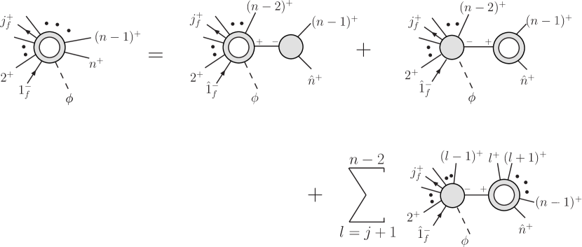
Figure 7: Diagrams corresponding to the terms in the recursion relation (133) for $A_{n}^{s}(\phi,j_{\!f}^{+})$. The second diagram contains a double pole, and an unreal pole underneath it. In the last diagram, the sum over $l$ runs from $j+1$ to $n-2$, inclusive.

The recursion relation for the corresponding single-$\phi$ amplitudes, $A_{n}^{s}(\phi,j_{\!f}^{+})$, depicted in fig. 7, is very similar,

$$\hbox{}\hskip-14.22636ptA_{n}^{s}(\phi,j_{\!f}^{+})=$$

$$A_{n-1}^{s}(\phi,\hat{1}_{\!f}^{-},2^{+},\ldots,j_{\!f}^{+},\ldots,(n-2)^{+},{\hat{K}}_{n-1,n}^{+})\,{i\over s_{n-1,n}}\,A_{3}^{{(0)}}(-{\hat{K}}_{n-1,n}^{-},(n-1)^{+},\hat{n}^{+})$$

$$\hbox{}+A_{n-1}^{(0)}(\phi,\hat{1}_{\!f}^{-},2^{+},\ldots,j_{\!f}^{+},\ldots,(n-2)^{+},{\hat{K}}_{n-1,n}^{-})\,{i\over s_{n-1,n}^{2}}\,V_{3}^{{(1)}}(-{\hat{K}}_{n-1,n}^{+},(n-1)^{+},\hat{n}^{+})$$

$$\hskip 14.22636pt\hbox{}\times\Bigl{(}1+s_{n-1,n}\,{\cal S}^{(0)}(n-2,{\hat{K}}_{n-1,n}^{+},j)\,{\cal S}^{(0)}(\hat{n},-{\hat{K}}_{n-1,n}^{-},n-1)\Bigr{)}$$

$$\hbox{}+\sum_{l=j+1}^{n-2}A_{l}^{(0)}(\phi,\hat{1}_{\!f}^{-},2^{+},\ldots,j_{\!f}^{+},\ldots,(l-1)^{+},{\hat{K}}_{l\cdots n}^{-})\,{i\over s_{l\cdots n}}\,A_{n-l+2}^{{(1)}}(-{\hat{K}}_{l\cdots n}^{+},l^{+},\ldots,\hat{n}^{+})\,.$$

(133)

Notice that in this case $\phi$ only makes its appearance in the “source terms” — the second and third terms in fig. 7 — through tree amplitudes. Recall also that the relevant $\phi$-containing MHV tree amplitudes (79) are identical in form to the ones without $\phi$, eq. (60). Thus we should expect the solution to the recursion relation to have essentially the same form as in the pure-QCD case.

Indeed, the solution to eq. (133) is

$$A_{n}^{s}(\phi;j_{\!f}^{+})={i\over 3}{S_{1}^{\phi}+S_{2}^{\phi}\over\left\langle 1\,2\right\rangle\left\langle 2\,3\right\rangle\cdots\left\langle n\,1\right\rangle}\,,$$ (134)

where

$$S_{1}^{\phi} = \sum_{l=j+1}^{n-1}{\left\langle j\,l\right\rangle\left\langle 1\,(l+1)\right\rangle\left\langle\smash{1}{\vphantom{1}}^{-}\right|{{\raise 0.91666pt\hbox to9.20833pt{\hss/\hss}\hbox to0.0pt{\hss$K$}}_{l,l+1}{\raise 0.91666pt\hbox to9.20833pt{\hss/\hss}\hbox to0.0pt{\hss$K$}}_{(l+1)\cdots n}}\left|\smash{1}{\vphantom{1}}^{+}\right\rangle\over\left\langle l\,(l+1)\right\rangle}\,,$$ (135)

$$S_{2}^{\phi} = -\sum_{l=j+1}^{n-2}\sum_{p=l+1}^{n-1}{\left\langle(l-1)\,l\right\rangle\over\left\langle\smash{1}{\vphantom{1}}^{-}\right|{{\raise 0.91666pt\hbox to9.20833pt{\hss/\hss}\hbox to0.0pt{\hss$K$}}_{(p+1)\cdots n}{\raise 0.91666pt\hbox to9.20833pt{\hss/\hss}\hbox to0.0pt{\hss$K$}}_{l\cdots p}}\left|\smash{(l-1)}{\vphantom{1}}^{+}\right\rangle\left\langle\smash{1}{\vphantom{1}}^{-}\right|{{\raise 0.91666pt\hbox to9.20833pt{\hss/\hss}\hbox to0.0pt{\hss$K$}}_{(p+1)\cdots n}{\raise 0.91666pt\hbox to9.20833pt{\hss/\hss}\hbox to0.0pt{\hss$K$}}_{l\cdots p}}\left|\smash{l}{\vphantom{1}}^{+}\right\rangle}$$ (136)

$$\hskip 42.67912pt\times{\left\langle p\,(p+1)\right\rangle\over\left\langle\smash{1}{\vphantom{1}}^{-}\right|{{\raise 0.91666pt\hbox to9.20833pt{\hss/\hss}\hbox to0.0pt{\hss$K$}}_{l\cdots n}{\raise 0.91666pt\hbox to9.20833pt{\hss/\hss}\hbox to0.0pt{\hss$K$}}_{l\cdots p}}\left|\smash{p}{\vphantom{1}}^{+}\right\rangle\left\langle\smash{1}{\vphantom{1}}^{-}\right|{{\raise 0.91666pt\hbox to9.20833pt{\hss/\hss}\hbox to0.0pt{\hss$K$}}_{l\cdots n}{\raise 0.91666pt\hbox to9.20833pt{\hss/\hss}\hbox to0.0pt{\hss$K$}}_{l\cdots p}}\left|\smash{(p+1)}{\vphantom{1}}^{+}\right\rangle}$$

$$\hskip 42.67912pt\times{\left\langle\smash{1}{\vphantom{1}}^{-}\right|{{\raise 0.91666pt\hbox to9.20833pt{\hss/\hss}\hbox to0.0pt{\hss$K$}}_{l\cdots p}{\raise 0.91666pt\hbox to9.20833pt{\hss/\hss}\hbox to0.0pt{\hss$K$}}_{(p+1)\cdots n}}\left|\smash{1}{\vphantom{1}}^{+}\right\rangle}^{2}\left\langle\smash{j}{\vphantom{1}}^{-}\right|{{\raise 0.91666pt\hbox to9.20833pt{\hss/\hss}\hbox to0.0pt{\hss$K$}}_{l\cdots p}{\raise 0.91666pt\hbox to9.20833pt{\hss/\hss}\hbox to0.0pt{\hss$K$}}_{(p+1)\cdots n}}\left|\smash{1}{\vphantom{1}}^{+}\right\rangle$$

$$\hskip 42.67912pt\times{\left\langle\smash{1}{\vphantom{1}}^{-}\right|{{\raise 0.91666pt\hbox to9.20833pt{\hss/\hss}\hbox to0.0pt{\hss$K$}}_{l\cdots n}[{\cal F}(l,p)]^{2}{\raise 0.91666pt\hbox to9.20833pt{\hss/\hss}\hbox to0.0pt{\hss$K$}}_{(p+1)\cdots n}}\left|\smash{1}{\vphantom{1}}^{+}\right\rangle\over s_{l\cdots p}}\,.$$

The $S_{1}^{\phi}$ term manifestly has the same form as the pure-QCD result $S_{1}$ in eq. (74), apart from the implicit $\phi$ momentum. For the $S_{2}^{\phi}$ term, we use momentum conservation to substitute

$${\raise 0.91666pt\hbox to9.20833pt{\hss/\hss}\hbox to0.0pt{\hss$K$}}_{2\cdots(l-1)}=-{\raise 0.91666pt\hbox to9.20833pt{\hss/\hss}\hbox to0.0pt{\hss$K$}}_{l\cdots n}\,,$$ (137)

in the expression for $S_{2}$ in eq. (75). Then the $S_{2}^{\phi}$ term is identical in form to $S_{2}$ as well.

Because of the simple relation between $S_{i}^{\phi}$ and $S_{i}$, it is trivial to show that the solution (134) for $A_{n}^{s}(\phi,j_{\!f}^{+})$, like the solution (113) for $A_{n}^{L-s}(\phi,j_{\!f}^{+})$, obeys the expected soft-Higgs limit (100) with $n_{-}=1$,

$$A_{n}^{s}(\phi,j_{\!f}^{+})\longrightarrow A_{n}^{s}(j_{\!f}^{+})\qquad\quad\hbox{as $k_{\phi}\to 0$.}$$ (138)

The simple relation between $S_{i}^{\phi}$ and $S_{i}$ also makes it very easy to demonstrate that the set of amplitudes $A_{n}^{s}(\phi,j_{\!f}^{+})$ given in eq. (134) satisfy the recursion relation (133). We just use the analysis in section V D of ref. LastFinite , which proved the analogous result for QCD, namely that $A_{n}^{s}(j_{\!f}^{+})$ as given in eq. (73) satisfies the recursion relation (131). The only modification that needs to be made to the arguments and identities is that ${\raise 0.91666pt\hbox to9.20833pt{\hss/\hss}\hbox to0.0pt{\hss$K$}}_{2\cdots(l-1)}$ should be replaced by $-{\raise 0.91666pt\hbox to9.20833pt{\hss/\hss}\hbox to0.0pt{\hss$K$}}_{l\cdots n}$ everywhere, according to eq. (137). After doing that, all expressions appearing in the two recursion relations and solutions, for $A_{n}^{s}$ with $\phi$ and without, have exactly the same form. The momentum of $\phi$ only appears implicitly in $A_{n}(\phi,j_{\!f}^{+})$, through momentum conservation. In addition, after replacing ${\raise 0.91666pt\hbox to9.20833pt{\hss/\hss}\hbox to0.0pt{\hss$K$}}_{2\cdots(l-1)}$, none of the identities used in ref. LastFinite require momentum conservation (which could have introduced the $\phi$ momentum). In the analysis of the contribution of the $l^{\rm th}$ term in the last diagram of fig. 7, for example, only legs $l$ to $n$ are involved in an essential way.

VII.4 Factorization properties of solution, and a $\phi$-plus-$n$-gluon amplitude

In appendix A of ref. LastFinite it was shown that the pure-QCD formula (73) has all the correct multiparticle poles, factorizing properly onto products of the quark-containing MHV tree amplitudes (60) and the one-loop all-plus pure-gluon amplitudes (61). The corresponding demonstration for the $\phi$ amplitude $A_{n}^{s}(\phi,j_{\!f}^{+})$ is completely analogous, so we do not present it here. The collinear singularities of eqs. (113) and (134) work in exactly the same way; there are no collinear singularities between the $\phi$ particle and another parton, only between pairs of partons, and the corresponding $(n-1)$-point amplitudes again have exactly the same form as in the pure-QCD case. By taking the anti-quark and quark to be collinear in the amplitude in which they are adjacent ($j=2$), we can extract the scalar and $[g-s]$ loop contributions to the one-loop amplitudes for $\phi g^{\pm}g^{+}\ldots g^{+}$.

A term containing $1/\left[1\,2\right]$, corresponding to the splitting amplitude $\mathop{\rm Split}\nolimits_{-}^{(0)}(1_{f}^{-},2_{f}^{+};z)$, indicates a factorization onto the all-plus amplitude, $\phi g^{+}g^{+}\ldots g^{+}$. We observe that eq. (134) for $A_{n}^{s}(\phi,2_{f}^{+})$ does not contain a factor of $1/\left[1\,2\right]$, thus confirming the observation in section VI that the scalar $\phi$-amplitude with gluons of positive helicity vanishes, eq. (101). Similarly, in this collinear limit, $A_{n}^{L-s}(\phi,2_{f}^{+})$ as given in eq. (113) factorizes onto the gluonic $\phi$-all-plus amplitudes, eq. (102). The relevant contribution comes from the term with $l=3$ and $p=n$ of $Q_{2}^{\phi}$, as given in eq. (116).

Analogously, we can extract the scalar and $[g-s]$ contributions to the amplitude for a $\phi$ plus $n$ gluons, one of which has negative helicity, from eqs. (134) and (113), respectively. The result for the scalar contribution is,

$$A_{n}^{[s]}(\phi,1^{-},2^{+},3^{+},\ldots,n^{+})={i\over 3}{T_{1}^{\phi}+T_{2}^{\phi}\over\left\langle 1\,2\right\rangle\left\langle 2\,3\right\rangle\cdots\left\langle n\,1\right\rangle}\,,$$ (139)

where

$$T_{1}^{\phi} = \sum_{l=2}^{n-1}{\left\langle 1\,l\right\rangle\left\langle 1\,(l+1)\right\rangle\left\langle\smash{1}{\vphantom{1}}^{-}\right|{{\raise 0.91666pt\hbox to9.20833pt{\hss/\hss}\hbox to0.0pt{\hss$K$}}_{l,l+1}{\raise 0.91666pt\hbox to9.20833pt{\hss/\hss}\hbox to0.0pt{\hss$K$}}_{(l+1)\cdots n}}\left|\smash{1}{\vphantom{1}}^{+}\right\rangle\over\left\langle l\,(l+1)\right\rangle}\,,$$ (140)

$$T_{2}^{\phi} = -\,\sum_{l=2}^{n-2}\sum_{p=l+1}^{n-1}{\left\langle(l-1)\,l\right\rangle\over\left\langle\smash{1}{\vphantom{1}}^{-}\right|{{\raise 0.91666pt\hbox to9.20833pt{\hss/\hss}\hbox to0.0pt{\hss$K$}}_{(p+1)\cdots n}{\raise 0.91666pt\hbox to9.20833pt{\hss/\hss}\hbox to0.0pt{\hss$K$}}_{l\cdots p}}\left|\smash{(l-1)}{\vphantom{1}}^{+}\right\rangle\left\langle\smash{1}{\vphantom{1}}^{-}\right|{{\raise 0.91666pt\hbox to9.20833pt{\hss/\hss}\hbox to0.0pt{\hss$K$}}_{(p+1)\cdots n}{\raise 0.91666pt\hbox to9.20833pt{\hss/\hss}\hbox to0.0pt{\hss$K$}}_{l\cdots p}}\left|\smash{l}{\vphantom{1}}^{+}\right\rangle}$$ (141)

$$\hskip 42.67912pt\times{\left\langle p\,(p+1)\right\rangle\over\left\langle\smash{1}{\vphantom{1}}^{-}\right|{{\raise 0.91666pt\hbox to9.20833pt{\hss/\hss}\hbox to0.0pt{\hss$K$}}_{l\cdots n}{\raise 0.91666pt\hbox to9.20833pt{\hss/\hss}\hbox to0.0pt{\hss$K$}}_{l\cdots p}}\left|\smash{p}{\vphantom{1}}^{+}\right\rangle\left\langle\smash{1}{\vphantom{1}}^{-}\right|{{\raise 0.91666pt\hbox to9.20833pt{\hss/\hss}\hbox to0.0pt{\hss$K$}}_{l\cdots n}{\raise 0.91666pt\hbox to9.20833pt{\hss/\hss}\hbox to0.0pt{\hss$K$}}_{l\cdots p}}\left|\smash{(p+1)}{\vphantom{1}}^{+}\right\rangle}$$

$$\hskip 42.67912pt\times{\left\langle\smash{1}{\vphantom{1}}^{-}\right|{{\raise 0.91666pt\hbox to9.20833pt{\hss/\hss}\hbox to0.0pt{\hss$K$}}_{l\cdots p}{\raise 0.91666pt\hbox to9.20833pt{\hss/\hss}\hbox to0.0pt{\hss$K$}}_{(p+1)\cdots n}}\left|\smash{1}{\vphantom{1}}^{+}\right\rangle}^{3}$$

$$\hskip 42.67912pt\times{\left\langle\smash{1}{\vphantom{1}}^{-}\right|{{\raise 0.91666pt\hbox to9.20833pt{\hss/\hss}\hbox to0.0pt{\hss$K$}}_{l\cdots n}[{\cal F}(l,p)]^{2}{\raise 0.91666pt\hbox to9.20833pt{\hss/\hss}\hbox to0.0pt{\hss$K$}}_{(p+1)\cdots n}}\left|\smash{1}{\vphantom{1}}^{+}\right\rangle\over s_{l\cdots p}}\,.$$

Similarly, from eq. (113) we obtain for the $[g-s]$ contribution,

$$A_{n}^{[g-s]}(\phi,1^{-},2^{+},\ldots,n^{+})={i\over 2}{R_{1}^{\phi}+R_{2}^{\phi}\over\left\langle 1\,2\right\rangle\left\langle 2\,3\right\rangle\cdots\left\langle n\,1\right\rangle}\,,$$ (142)

where

$$R_{1}^{\phi} = -4\sum_{l=3}^{n}{\left\langle(l-1)\,l\right\rangle\,{\left\langle\smash{1}{\vphantom{1}}^{-}\right|{{\raise 0.91666pt\hbox to9.20833pt{\hss/\hss}\hbox to0.0pt{\hss$K$}}_{l\cdots n}{\raise 0.97221pt\hbox to5.52084pt{\hss/\hss}\hbox to0.0pt{\hss$k$}}_{\phi}}\left|\smash{1}{\vphantom{1}}^{+}\right\rangle}^{3}\over\left\langle\smash{1}{\vphantom{1}}^{-}\right|{{\raise 0.91666pt\hbox to9.20833pt{\hss/\hss}\hbox to0.0pt{\hss$K$}}_{l\cdots n}{\raise 0.97221pt\hbox to5.52084pt{\hss/\hss}\hbox to0.0pt{\hss$k$}}_{\phi}}\left|\smash{(l-1)}{\vphantom{1}}^{+}\right\rangle\left\langle\smash{1}{\vphantom{1}}^{-}\right|{{\raise 0.91666pt\hbox to9.20833pt{\hss/\hss}\hbox to0.0pt{\hss$K$}}_{2\cdots(l-1)}{\raise 0.97221pt\hbox to5.52084pt{\hss/\hss}\hbox to0.0pt{\hss$k$}}_{\phi}}\left|\smash{l}{\vphantom{1}}^{+}\right\rangle}\,,$$ (143)

$$R_{2}^{\phi} = -4\sum_{l=3}^{n-1}\sum_{p=l}^{n-1}{\left\langle(l-1)\,l\right\rangle\over\left\langle\smash{1}{\vphantom{1}}^{-}\right|{{\raise 0.91666pt\hbox to9.20833pt{\hss/\hss}\hbox to0.0pt{\hss$K$}}_{(p+1)\cdots n}{\raise 0.91666pt\hbox to9.20833pt{\hss/\hss}\hbox to0.0pt{\hss$K$}}_{\phi,l\cdots p}}\left|\smash{(l-1)}{\vphantom{1}}^{+}\right\rangle\left\langle\smash{1}{\vphantom{1}}^{-}\right|{{\raise 0.91666pt\hbox to9.20833pt{\hss/\hss}\hbox to0.0pt{\hss$K$}}_{(p+1)\cdots n}{\raise 0.91666pt\hbox to9.20833pt{\hss/\hss}\hbox to0.0pt{\hss$K$}}_{\phi,l\cdots p}}\left|\smash{l}{\vphantom{1}}^{+}\right\rangle}$$ (144)

$$\hskip 17.07164pt\hbox{}\times{\left\langle p\,(p+1)\right\rangle\over\left\langle\smash{1}{\vphantom{1}}^{-}\right|{{\raise 0.91666pt\hbox to9.20833pt{\hss/\hss}\hbox to0.0pt{\hss$K$}}_{2\cdots(l-1)}{\raise 0.91666pt\hbox to9.20833pt{\hss/\hss}\hbox to0.0pt{\hss$K$}}_{\phi,l\cdots p}}\left|\smash{p}{\vphantom{1}}^{+}\right\rangle\left\langle\smash{1}{\vphantom{1}}^{-}\right|{{\raise 0.91666pt\hbox to9.20833pt{\hss/\hss}\hbox to0.0pt{\hss$K$}}_{2\cdots(l-1)}{\raise 0.91666pt\hbox to9.20833pt{\hss/\hss}\hbox to0.0pt{\hss$K$}}_{\phi,l\cdots p}}\left|\smash{(p+1)}{\vphantom{1}}^{+}\right\rangle}$$

$$\hskip 17.07164pt\hbox{}\times{\left\langle\smash{1}{\vphantom{1}}^{-}\right|{{\raise 0.91666pt\hbox to9.20833pt{\hss/\hss}\hbox to0.0pt{\hss$K$}}_{(p+1)\cdots n}{\raise 0.91666pt\hbox to9.20833pt{\hss/\hss}\hbox to0.0pt{\hss$K$}}_{\phi,l\cdots p}}\left|\smash{1}{\vphantom{1}}^{+}\right\rangle}^{4}\ {(k_{\phi}^{2})^{2}\over s_{\phi,l\cdots p}}\,.$$

As indicated by eq. (18), and as explained in section VI, the amplitude with a fermion in the loop, $A_{n}^{[f]}(\phi,1^{-},2^{+},3^{+},\ldots,n^{+})$, is equal and opposite in sign to the scalar-loop contribution $A_{n}^{[s]}(\phi,1^{-},2^{+},3^{+},\ldots,n^{+})$ given in eq. (139). The soft Higgs limit of eqs. (139) and (142) onto the corresponding pure-QCD amplitudes (68) can easily be verified to obey eq. (100), just as in the quark case.

Equation (142) completes the construction of all the finite one-loop QCD amplitudes containing a $\phi$ field plus multiple partons.

VIII Results for two, three and four partons

In this section we collect explicit analytical results for up to four partons, using formulæ from the previous section, as well as some results for divergent helicity configurations which have appeared elsewhere, in particular in refs. Schmidt ; BadgerGloverH4g .

VIII.1 Complete results for two and three partons

In appendix A, eqs. (190), (191), and (192), we record the complete set of $\phi gg$ amplitudes, $\phi g^{+}g^{+}$, $\phi g^{\mp}g^{\pm}$, and $\phi g^{-}g^{-}$. The $\phi\bar{q}q$ amplitudes vanish (for massless quarks) by angular momentum conservation, so, rather trivially, we have the complete set of amplitudes for a single $\phi$ plus 2 partons.

The purpose of this subsection is to give the complete set of amplitudes for a single $\phi$ plus 3 partons. We start with the $\phi ggg$ amplitudes. In the color decomposition (12), there is only one color structure, corresponding to the partial amplitude $A_{3;1}$. First we record the finite helicity configurations, using our all-$n$ results. Then, using these formulæ and eq. (6), we decompose the one-loop $Hggg$-amplitudes computed in ref. Schmidt into $\phi ggg$ and $\phi^{\dagger}ggg$ amplitudes. Finally we use parity to recast the results just in terms of $\phi ggg$ amplitudes. These amplitudes will play a role in the recursive construction of one-loop Higgs amplitudes with more external partons.

We express the one-loop results in terms of the corresponding $Hggg$ or $\phi^{\dagger}ggg$ tree-level amplitudes,

$$A_{3}^{(0)}(H,1^{+},2^{+},3^{+})=A_{3}^{(0)}(\phi^{\dagger},1^{+},2^{+},3^{+}) = i\frac{(k_{\phi}^{2})^{2}}{\left\langle 1\,2\right\rangle\left\langle 2\,3\right\rangle\left\langle 3\,1\right\rangle}\,,$$ (145)

$$A_{3}^{(0)}(H,1^{-},2^{+},3^{+})=A_{3}^{(0)}(\phi^{\dagger},1^{-},2^{+},3^{+}) = -i\frac{\left[2\,3\right]^{3}}{\left[1\,2\right]\left[3\,1\right]}\,.$$ (146)

These amplitudes can be read off from eqs. (76), (78), and (84), with the help of eqs. (6) and (8). The $[s]$ and $[g-s]$ components of the finite loop amplitudes are, using eqs. (101), (102), (139), and (142),

$$A_{3}^{[s]}(\phi,1^{+},2^{+},3^{+}) = 0\,,$$ (147)

$$A_{3}^{[g-s]}(\phi,1^{+},2^{+},3^{+}) = -2\,A_{3}^{(0)}(\phi^{\dagger},1^{+},2^{+},3^{+})\,,$$ (148)

$$A_{3}^{[s]}(\phi,1^{-},2^{+},3^{+}) = \frac{1}{3}\frac{s_{31}s_{12}}{s_{23}^{2}}A_{3}^{(0)}(\phi^{\dagger},1^{-},2^{+},3^{+})\,,$$ (149)

$$A_{3}^{[g-s]}(\phi,1^{-},2^{+},3^{+}) = -2A_{3}^{(0)}(\phi^{\dagger},1^{-},2^{+},3^{+})\,.$$ (150)

Using eq. (18), the full $\phi ggg$ one-loop amplitudes are,

$$A_{3;1}(\phi,1^{+},2^{+},3^{+}) = -2\,A_{3}^{(0)}(\phi^{\dagger},1^{+},2^{+},3^{+})\,,$$ (151)

$$A_{3;1}(\phi,1^{-},2^{+},3^{+}) = A_{3}^{(0)}(\phi^{\dagger},1^{-},2^{+},3^{+})\left[-2+\frac{1}{3}\left(1-\frac{n_{\!f}}{N_{c}}+\frac{n_{s}}{N_{c}}\right)\frac{s_{31}s_{12}}{s_{23}^{2}}\right]\,.$$ (152)

The one-loop $Hggg$ amplitudes are Schmidt , in our notation,

$$A_{3;1}(H,1^{+},2^{+},3^{+}) = A_{3}^{(0)}(\phi^{\dagger},1^{+},2^{+},3^{+})\Biggl{[}U_{3}+{1\over 3}\biggl{(}1-{n_{\!f}\over N_{c}}+{n_{s}\over N_{c}}\biggr{)}{s_{12}s_{23}+s_{23}s_{31}+s_{31}s_{12}\over(k_{\phi}^{2})^{2}}\Biggr{]}\,,$$

$$A_{3;1}(H,1^{-},2^{+},3^{+}) = A_{3}^{(0)}(\phi^{\dagger},1^{-},2^{+},3^{+})\Biggl{[}U_{3}+{1\over 3}\biggl{(}1-{n_{\!f}\over N_{c}}+{n_{s}\over N_{c}}\biggr{)}{s_{31}s_{12}\over s_{23}^{2}}\Biggr{]}\,,$$ (154)

where

$$U_{3} \equiv -{1\over\epsilon^{2}}\Biggl{[}\biggl{(}{\mu^{2}\over-s_{12}}\biggr{)}^{\epsilon}+\biggl{(}{\mu^{2}\over-s_{23}}\biggr{)}^{\epsilon}+\biggl{(}{\mu^{2}\over-s_{31}}\biggr{)}^{\epsilon}\Biggr{]}+{\pi^{2}\over 2}$$ (155)

$$\hskip 0.0pt-\ln\biggl{(}{-s_{12}\over-k_{\phi}^{2}}\biggr{)}\ln\biggl{(}{-s_{23}\over-k_{\phi}^{2}}\biggr{)}-\ln\biggl{(}{-s_{23}\over-k_{\phi}^{2}}\biggr{)}\ln\biggl{(}{-s_{31}\over-k_{\phi}^{2}}\biggr{)}-\ln\biggl{(}{-s_{31}\over-k_{\phi}^{2}}\biggr{)}\ln\biggl{(}{-s_{12}\over-k_{\phi}^{2}}\biggr{)}$$

$$\hskip 0.0pt-2\,\mathop{\rm Li}\nolimits_{2}\biggl{(}1-{s_{12}\over k_{\phi}^{2}}\biggr{)}-2\,\mathop{\rm Li}\nolimits_{2}\biggl{(}1-{s_{23}\over k_{\phi}^{2}}\biggr{)}-2\,\mathop{\rm Li}\nolimits_{2}\biggl{(}1-{s_{31}\over k_{\phi}^{2}}\biggr{)}$$

$$= -{1\over\epsilon^{2}}\Biggl{[}\biggl{(}{\mu^{2}\over-s_{12}}\biggr{)}^{\epsilon}+\biggl{(}{\mu^{2}\over-s_{23}}\biggr{)}^{\epsilon}+\biggl{(}{\mu^{2}\over-s_{31}}\biggr{)}^{\epsilon}\Biggr{]}$$

$$\hskip 0.0pt-\mathop{\rm Ls}\nolimits_{-1}\biggl{(}{-s_{12}\over-k_{\phi}^{2}},{-s_{23}\over-k_{\phi}^{2}}\biggr{)}-\mathop{\rm Ls}\nolimits_{-1}\biggl{(}{-s_{23}\over-k_{\phi}^{2}},{-s_{31}\over-k_{\phi}^{2}}\biggr{)}-\mathop{\rm Ls}\nolimits_{-1}\biggl{(}{-s_{31}\over-k_{\phi}^{2}},{-s_{12}\over-k_{\phi}^{2}}\biggr{)}\,,$$

with $k_{\phi}^{2}=s_{123}$, and $\mu$ is the scale originating from dimensional regularization. The one-mass box function $\mathop{\rm Ls}\nolimits_{-1}(r_{1},r_{2})$ is defined as eeFourPartons ,

$$\mathop{\rm Ls}\nolimits_{-1}(r_{1},r_{2})\equiv\mathop{\rm Li}\nolimits_{2}(1-r_{1})+\mathop{\rm Li}\nolimits_{2}(1-r_{2})+\ln r_{1}\ln r_{2}-{\pi^{2}\over 6}\,.$$ (156)

We have extended the results of ref. Schmidt to nonzero values of $n_{s}$ by observing that the $n_{\!f}$ and $n_{s}$ terms are proportional to an amplitude for an off-shell gluon to split, via a fermion or scalar loop, into two on-shell, identical-helicity gluons. (The opposite-helicity case vanishes.) Such contributions are opposite in sign for fermions and scalars, as can be seen by contracting the off-shell gluon with an external $\bar{q}q$ pair, and then using a supersymmetry identity SWI .

Using eq. (6), and subtracting eq. (151) from eq. (LABEL:Hppp1l), and eq. (152) from eq. (154), we have,

$$A_{3;1}(\phi^{\dagger},1^{+},2^{+},3^{+}) = A_{3}^{(0)}(\phi^{\dagger},1^{+},2^{+},3^{+})$$ (157)

$$\hskip 8.5359pt\times\Biggl{[}U_{3}+2+{1\over 3}\biggl{(}1-{n_{\!f}\over N_{c}}+{n_{s}\over N_{c}}\biggr{)}{s_{12}s_{23}+s_{23}s_{31}+s_{31}s_{12}\over(k_{\phi}^{2})^{2}}\Biggr{]}\,,~{}~{}~{}~{}$$

$$A_{3;1}(\phi^{\dagger},1^{-},2^{+},3^{+}) = A_{3}^{(0)}(\phi^{\dagger},1^{-},2^{+},3^{+})[U_{3}+2]\,.$$ (158)

The parity conjugates of these results constitute the remaining helicity amplitudes for $\phi$ plus three gluons,

$$A_{3;1}(\phi,1^{-},2^{-},3^{+}) = A_{3}^{(0)}(\phi,1^{-},2^{-},3^{+})[U_{3}+2]\,,$$ (159)

$$A_{3;1}(\phi,1^{-},2^{-},3^{-}) = A_{3}^{(0)}(\phi,1^{-},2^{-},3^{-})$$ (160)

$$\hskip 8.5359pt\times\Biggl{[}U_{3}+2+{1\over 3}\biggl{(}1-{n_{\!f}\over N_{c}}+{n_{s}\over N_{c}}\biggr{)}{s_{12}s_{23}+s_{23}s_{31}+s_{31}s_{12}\over(k_{\phi}^{2})^{2}}\Biggr{]}\,.~{}~{}~{}~{}$$

It is trivial to obtain the corresponding amplitudes for a pseudoscalar $A$ plus three gluons via eq. (7),

$$A_{3;1}(A,1^{+},2^{+},3^{+}) = i\,A_{3}^{(0)}(\phi^{\dagger},1^{+},2^{+},3^{+})$$ (161)

$$\hskip 8.5359pt\times\Biggl{[}U_{3}+4+{1\over 3}\,\biggl{(}1-{n_{\!f}\over N_{c}}+{n_{s}\over N_{c}}\biggr{)}{s_{12}s_{23}+s_{23}s_{31}+s_{31}s_{12}\over(k_{\phi}^{2})^{2}}\Biggr{]}\,,~{}~{}~{}~{}~{}$$

$$A_{3;1}(A,1^{-},2^{+},3^{+}) = i\,A_{3}^{(0)}(\phi^{\dagger},1^{-},2^{+},3^{+})\Biggl{[}U_{3}+4-{1\over 3}\biggl{(}1-{n_{\!f}\over N_{c}}+{n_{s}\over N_{c}}\biggr{)}{s_{31}s_{12}\over s_{23}^{2}}\Biggr{]}\,.$$ (162)

Let us now turn to the $\phi\bar{q}qg$ amplitudes. There is only one nonvanishing color structure in eq. (21), with partial amplitude $A_{3;1}$. We again express the one-loop results in terms of the corresponding $H\bar{q}qg$, or equivalently, $\phi^{\dagger}\bar{q}qg$ tree amplitude,

$$A_{3}^{(0)}(H,1_{f}^{-},2_{f}^{+},3^{+})=A_{3}^{(0)}(\phi^{\dagger},1_{f}^{-},2_{f}^{+},3^{+})=-i\frac{\left[2\,3\right]^{2}}{\left[1\,2\right]}\,.$$ (163)

This amplitude can be obtained from eqs. (77) and (79), by using eqs. (6) and (8). We find from eq. (113),

$$A_{3}^{L-s}(\phi,1_{f}^{-},2_{f}^{+},3^{+})=2\,i\,\frac{\left[2\,3\right]^{2}}{\left[1\,2\right]}+{i\over 2}{\left\langle 1\,2\right\rangle\left[2\,3\right]\over\left\langle 2\,3\right\rangle}=-2A_{3}^{(0)}(\phi^{\dagger},1_{f}^{-},2_{f}^{+},3^{+})+{i\over 2}{\left\langle 1\,2\right\rangle\left[2\,3\right]\over\left\langle 2\,3\right\rangle}\,.$$ (164)

The corresponding scalar amplitude $A_{3}^{s}(\phi;1_{f}^{-},2_{f}^{+},3^{+})$ vanishes, but the $R$ type amplitude does not, $A_{3}^{R}(\phi,1_{f}^{-},2_{f}^{+},3^{+})=-A_{3}^{L}(\phi,1_{f}^{-},3^{+},2_{f}^{+})=-(i/2)\left\langle 1\,2\right\rangle\left[2\,3\right]/\left\langle 2\,3\right\rangle$. Equation (25) then gives the full $\phi\bar{q}qg$ one-loop amplitude as,

$$A_{3;1}(\phi,1_{f}^{-},2_{f}^{+},3^{+}) = -2A_{3}^{(0)}(\phi^{\dagger},1_{f}^{-},2_{f}^{+},3^{+})+{i\over 2}\left(1+{1\over N_{c}^{2}}\right){\left\langle 1\,2\right\rangle\left[2\,3\right]\over\left\langle 2\,3\right\rangle}$$ (165)

$$= A_{3}^{(0)}(\phi^{\dagger},1_{f}^{-},2_{f}^{+},3^{+})\left[-\,2-\left(1+{1\over N_{c}^{2}}\right){s_{12}\over 2\,s_{23}}\right]\,.$$

From the one-loop $H\bar{q}qg$ amplitude Schmidt and eq. (165) we can extract the corresponding $\phi^{\dagger}$-contribution as above. The $H\bar{q}qg$ amplitude is

$$A_{3;1}(H,1_{f}^{-},2_{f}^{+},3^{+})=A_{3}^{(0)}(\phi^{\dagger},1_{f}^{-},2_{f}^{+},3^{+})\Biggl{[}V_{1}+{1\over N_{c}^{2}}V_{2}+{n_{\!f}\over N_{c}}V_{3}+{n_{s}\over N_{c}}V_{4}\Biggr{]}\ ,$$ (166)

with

$$V_{1} \equiv -{1\over\epsilon^{2}}\biggl{[}\biggl{(}{\mu^{2}\over-s_{23}}\biggr{)}^{\epsilon}+\biggl{(}{\mu^{2}\over-s_{31}}\biggr{)}^{\epsilon}\biggr{]}\,+\,{13\over 6\epsilon}\biggl{(}{\mu^{2}\over-s_{12}}\biggr{)}^{\epsilon}$$ (167)

$$\hskip 0.0pt-\mathop{\rm Ls}\nolimits_{-1}\biggl{(}{-s_{12}\over-k_{\phi}^{2}},{-s_{23}\over-k_{\phi}^{2}}\biggr{)}-\mathop{\rm Ls}\nolimits_{-1}\biggl{(}{-s_{31}\over-k_{\phi}^{2}},{-s_{12}\over-k_{\phi}^{2}}\biggr{)}\,+\,{83\over 18}\,-\,{\delta_{R}\over 6}\,-\,{1\over 2}{s_{12}\over s_{23}}\ ,$$

$$V_{2} \equiv \biggl{[}{1\over\epsilon^{2}}+{3\over 2\epsilon}\biggr{]}\biggl{(}{\mu^{2}\over-s_{12}}\biggr{)}^{\epsilon}\,+\,\mathop{\rm Ls}\nolimits_{-1}\biggl{(}{-s_{23}\over-k_{\phi}^{2}},{-s_{31}\over-k_{\phi}^{2}}\biggr{)}\,+\,{7\over 2}\,+\,{\delta_{R}\over 2}\,-\,{1\over 2}{s_{12}\over s_{23}}\ ,$$ (168)

$$V_{3} \equiv -\,{2\over 3\epsilon}\biggl{(}{\mu^{2}\over-s_{12}}\biggr{)}^{\epsilon}\,-\,{10\over 9}\ ,$$ (169)

$$V_{4} \equiv -\,{1\over 3\epsilon}\biggl{(}{\mu^{2}\over-s_{12}}\biggr{)}^{\epsilon}\,-\,{8\over 9}\ .$$ (170)

Here $\delta_{R}$ is a regularization-scheme dependent parameter, which fixes the number of helicity states of the gluons running in the loop to $(4-2\delta_{R}\epsilon)$. For the ’t Hooft-Veltman scheme HV $\delta_{R}=1$, while in the four-dimensional helicity (FDH) scheme BKStringBased ; OtherFDH $\delta_{R}=0$. (Note that in the FDH scheme, the combination $V_{1}-V_{2}+V_{3}$ is equal to the function $U_{3}$ appearing in the $Hggg$ amplitude.) The $n_{s}$ term can be deduced from the $n_{\!f}$ term using the fact that both arise from vacuum-polarization contributions. For this helicity configuration, the fermion and scalar loop contributions are not equal and opposite in sign.

From eqs. (6), (165), and (166) then follows,

$$A_{3;1}(\phi^{\dagger},1_{f}^{-},2_{f}^{+},3^{+})=A_{3}^{(0)}(\phi^{\dagger},1_{f}^{-},2_{f}^{+},3^{+})\Biggl{[}V_{1}+{s_{12}\over 2\,s_{23}}+2+{1\over N_{c}^{2}}\left(V_{2}+{s_{12}\over 2\,s_{23}}\right)+{n_{\!f}\over N_{c}}V_{3}+{n_{s}\over N_{c}}V_{4}\Biggr{]}\,.$$ (171)

The $L$, $R$, $f$ and $s$ pieces of $A_{3;1}(\phi,1_{f}^{-},2_{f}^{+},3^{-})$ can easily be extracted from the various color components of eq. (171) after applying parity, eq. (8). Note that the $s_{12}/(2s_{23})$ terms in eq. (171) cancel similar terms in $V_{1}$ and $V_{2}$ in eqs. (167) and (168).

Using eq. (7), the corresponding amplitude with a pseudoscalar $A$ is found to be,

$$A_{3;1}(A,1_{f}^{-},2_{f}^{+},3^{+})=i\,A_{3}^{(0)}(\phi^{\dagger},1_{f}^{-},2_{f}^{+},3^{+})\Biggl{[}V_{1}+{s_{12}\over s_{23}}+4+{1\over N_{c}^{2}}\left(V_{2}+{s_{12}\over s_{23}}\right)+{n_{\!f}\over N_{c}}V_{3}+{n_{s}\over N_{c}}V_{4}\Biggr{]}\,.$$ (172)

VIII.2 Partial results for four partons

The finite helicity amplitudes for a $\phi$ plus four gluons are given by,

$$A_{4}^{[s]}(\phi,1^{+},2^{+},3^{+},4^{+}) = 0\,,$$ (173)

$$A_{4}^{[g-s]}(\phi,1^{+},2^{+},3^{+},4^{+}) = -2\,A_{4}^{(0)}(\phi^{\dagger},1^{+},2^{+},3^{+},4^{+})\,,$$ (174)

$$A_{4}^{[s]}(\phi,1^{-},2^{+},3^{+},4^{+}) = \frac{i}{3}\Biggl{[}-{\left\langle 1\,2\right\rangle\left[2\,3\right]{\left\langle 1\,3\right\rangle}^{2}\over{\left\langle 2\,3\right\rangle}^{2}\left\langle 3\,4\right\rangle\left\langle 4\,1\right\rangle}-{\left\langle 1\,4\right\rangle\left[4\,3\right]{\left\langle 1\,3\right\rangle}^{2}\over\left\langle 1\,2\right\rangle\left\langle 2\,3\right\rangle{\left\langle 3\,4\right\rangle}^{2}}$$ (175)

$$\hskip 14.22636pt+{\left\langle\smash{1}{\vphantom{1}}^{-}\right|{(2+3)}\left|\smash{4}{\vphantom{1}}^{-}\right\rangle\left\langle\smash{1}{\vphantom{1}}^{-}\right|{(3+4)}\left|\smash{2}{\vphantom{1}}^{-}\right\rangle\over\left\langle 2\,3\right\rangle\left\langle 3\,4\right\rangle\,s_{234}}\Biggr{]}\,,$$

$$A_{4}^{[g-s]}(\phi,1^{-},2^{+},3^{+},4^{+}) = -2\,i\,\Biggl{[}{{\left\langle\smash{1}{\vphantom{1}}^{-}\right|{(2+3)}\left|\smash{4}{\vphantom{1}}^{-}\right\rangle}^{3}\over\left\langle 1\,2\right\rangle\left\langle 2\,3\right\rangle\left\langle\smash{3}{\vphantom{1}}^{-}\right|{(1+2)}\left|\smash{4}{\vphantom{1}}^{-}\right\rangle\,s_{123}}$$ (176)

$$\hskip 25.6073pt+{{\left\langle\smash{1}{\vphantom{1}}^{-}\right|{(3+4)}\left|\smash{2}{\vphantom{1}}^{-}\right\rangle}^{3}\over\left\langle 3\,4\right\rangle\left\langle 4\,1\right\rangle\left\langle\smash{3}{\vphantom{1}}^{-}\right|{(1+4)}\left|\smash{2}{\vphantom{1}}^{-}\right\rangle\,s_{134}}$$

$$\hskip 25.6073pt+{(k_{\phi}^{2})^{2}\,{\left[2\,4\right]}^{4}\over\left[4\,1\right]\left[1\,2\right]\,\left\langle\smash{3}{\vphantom{1}}^{-}\right|{(1+2)}\left|\smash{4}{\vphantom{1}}^{-}\right\rangle\left\langle\smash{3}{\vphantom{1}}^{-}\right|{(1+4)}\left|\smash{2}{\vphantom{1}}^{-}\right\rangle\,s_{124}}\Biggr{]}\,.~{}~{}~{}~{}~{}~{}~{}$$

We have also computed the terms containing cuts in the following all-minus amplitude,

$$A_{4}^{[g-s]}(\phi,1^{-},2^{-},3^{-},4^{-})=A_{4}^{(0)}(\phi,1^{-},2^{-},3^{-},4^{-})[U_{4}+2]\,,$$ (177)

where

$$U_{4} \equiv -{1\over\epsilon^{2}}\Biggl{[}\biggl{(}{\mu^{2}\over-s_{12}}\biggr{)}^{\epsilon}+\biggl{(}{\mu^{2}\over-s_{23}}\biggr{)}^{\epsilon}+\biggl{(}{\mu^{2}\over-s_{34}}\biggr{)}^{\epsilon}+\biggl{(}{\mu^{2}\over-s_{41}}\biggr{)}^{\epsilon}\Biggr{]}$$ (178)

$$\hskip 0.0pt-\mathop{\rm Ls}\nolimits_{-1}\biggl{(}{-s_{12}\over-s_{123}},{-s_{23}\over-s_{123}}\biggr{)}-\mathop{\rm Ls}\nolimits_{-1}\biggl{(}{-s_{23}\over-s_{234}},{-s_{34}\over-s_{234}}\biggr{)}$$

$$\hskip 0.0pt-\mathop{\rm Ls}\nolimits_{-1}\biggl{(}{-s_{34}\over-s_{341}},{-s_{41}\over-s_{341}}\biggr{)}-\mathop{\rm Ls}\nolimits_{-1}\biggl{(}{-s_{41}\over-s_{412}},{-s_{12}\over-s_{412}}\biggr{)}$$

$$\hskip 0.0pt-\mathop{\rm Ls}\nolimits_{-1}^{2{\rm m}e}(s_{123},s_{234};s_{23},k_{\phi}^{2})-\mathop{\rm Ls}\nolimits_{-1}^{2{\rm m}e}(s_{234},s_{341};s_{34},k_{\phi}^{2})$$

$$\hskip 0.0pt-\mathop{\rm Ls}\nolimits_{-1}^{2{\rm m}e}(s_{341},s_{412};s_{41},k_{\phi}^{2})-\mathop{\rm Ls}\nolimits_{-1}^{2{\rm m}e}(s_{412},s_{123};s_{12},k_{\phi}^{2})\,.$$

The two-mass box function $\mathop{\rm Ls}\nolimits_{-1}^{2{\rm m}e}(s,t;m_{1}^{2},m_{3}^{2})$ is defined as eeFourPartons ,

$$\mathop{\rm Ls}\nolimits_{-1}^{2{\rm m}e}(s,t;m_{1}^{2},m_{3}^{2}) \equiv -\mathop{\rm Li}\nolimits_{2}\left(1-{m_{1}^{2}\over s}\right)-\mathop{\rm Li}\nolimits_{2}\left(1-{m_{1}^{2}\over t}\right)-\mathop{\rm Li}\nolimits_{2}\left(1-{m_{3}^{2}\over s}\right)-\mathop{\rm Li}\nolimits_{2}\left(1-{m_{3}^{2}\over t}\right)$$ (179)

$$\hskip 0.0pt+\mathop{\rm Li}\nolimits_{2}\left(1-{m_{1}^{2}m_{3}^{2}\over st}\right)-{1\over 2}\ln^{2}\left({-s\over-t}\right)\,.$$

This result agrees with the all-$n$ cut-constructible expression $A_{n}^{(1),CC}$ found previously in ref. BadgerGloverH4g , when one substitutes $n=4$. As in the case of the $Hggg$ amplitudes, the “$2$” added to $U_{4}$ in eq. (177) for $A_{4}^{[g-s]}(\phi,1^{-},2^{-},3^{-},4^{-})$ cancels against a “$-2$” in $A_{4}^{[g-s]}(\phi^{\dagger},1^{-},2^{-},3^{-},4^{-})$ (the image under parity of $A_{4}^{[g-s]}(\phi,1^{+},2^{+},3^{+},4^{+})$ from eqs. (101) and (102)), when the $\phi$ and $\phi^{\dagger}$ amplitudes are added together to produce $A_{4}^{[g-s]}(H,1^{-},2^{-},3^{-},4^{-})$, or equivalently $A_{4}^{(1),CC}$ of ref. BadgerGloverH4g .

The non-cut-constructible contribution to this amplitude was computed in ref. BadgerGloverH4g . The result is

$$A_{4}^{[s]}(\phi,1^{-},2^{-},3^{-},4^{-}) = S^{----}(1,2,3,4)+S^{----}(2,3,4,1)$$ (180)

$$\hskip 0.0pt+\,S^{----}(3,4,1,2)+S^{----}(4,1,2,3)\,,$$

where

$$S^{----}(1,2,3,4) = {i\over 3}\Biggl{[}-\,{s_{13}\,{\left\langle\smash{4}{\vphantom{1}}^{-}\right|{(1+3)}\left|\smash{2}{\vphantom{1}}^{-}\right\rangle}^{2}\over{\left[1\,2\right]}^{2}{\left[2\,3\right]}^{2}\,s_{123}}+{{\left\langle 3\,4\right\rangle}^{2}\over{\left[1\,2\right]}^{2}}+2\,{\left\langle 3\,4\right\rangle\left\langle 4\,1\right\rangle\over\left[1\,2\right]\left[2\,3\right]}$$ (181)

$$\hskip 14.22636pt+\,{1\over 2}\,{s_{12}s_{34}+s_{123}s_{234}-s_{12}^{2}\over\left[1\,2\right]\left[2\,3\right]\left[3\,4\right]\left[4\,1\right]}\Biggr{]}\,,$$

and the four terms in eq. (180) are the images of $S^{----}(1,2,3,4)$ under cyclic permutations of the gluon legs. This result was computed as a gluon and fermion loop contribution, but it can be extended to incorporate a scalar loop contribution using factorization properties. We checked the collinear and multiparticle factorization limits of $A_{4}^{[g-s]}(\phi,1^{-},2^{-},3^{-},4^{-})$ and $A_{4}^{[s]}(\phi,1^{-},2^{-},3^{-},4^{-})$ onto the corresponding $\phi ggg$ and $\phi gg$ amplitudes.

The soft Higgs limit of the scalar loop term $A_{4}^{[s]}(\phi,1^{-},2^{-},3^{-},4^{-})$ in eq. (180) can easily be seen to obey eq. (100) with a factor of $n_{-}=4$. The target pure-QCD amplitude, from eq. (61), is

$$A_{4}^{[s]}(1^{-},2^{-},3^{-},4^{-})=-{i\over 3}{\left\langle 1\,2\right\rangle\left\langle 3\,4\right\rangle\over\left[1\,2\right]\left[3\,4\right]}\,.$$ (182)

Equivalently, the Higgs amplitude $A_{4}^{[s]}(H,1^{-},2^{-},3^{-},4^{-})$ obeys eq. (90) for $l=1$ and $n=4$, i.e. with a factor of $n+2l-2=4$ BadgerGloverH4g . The $[g-s]$ term $A_{4}^{[g-s]}(\phi,1^{-},2^{-},3^{-},4^{-})$ in eq. (177) vanishes in the soft limit, because the tree amplitude $A_{4}^{(0)}(1^{-},2^{-},3^{-},4^{-})$ vanishes, so that eqs. (98) and (99) for the soft limits of the divergent parts hold rather trivially.

Finally, the amplitude for a pseudoscalar $A$ plus four negative-helicity gluons is given via eq. (7) as

$$A_{4;1}(A,1^{-},2^{-},3^{-},4^{-}) = -i\,A_{4;1}(H,1^{-},2^{-},3^{-},4^{-})+2\,i\,A_{4}(\phi^{\dagger},1^{-},2^{-},3^{-},4^{-})~{}~{}~{}~{}$$ (184)

$$= -i\Biggl{[}A_{4}^{(0)}(\phi,1^{-},2^{-},3^{-},4^{-})[U_{4}+4]$$

$$\hskip 19.91684pt+\,\biggl{(}1-{n_{\!f}\over N_{c}}+{n_{s}\over N_{c}}\biggr{)}A_{4}^{[s]}(\phi,1^{-},2^{-},3^{-},4^{-})\Biggr{]}\,.$$

IX Conclusions

The production via gluon fusion of a Higgs boson in association with multiple jets provides an important background to Higgs production via electroweak vector boson fusion. Analytic representations of one-loop amplitudes containing a Higgs boson and four or more partons, interacting via the operator $H\mathop{\rm tr}\nolimits G_{\mu\nu}G^{\mu\nu}$, may be useful in quantifying this background. In this paper we have shown that on-shell recursive methods can be applied at the loop level, to amplitudes containing a complex $\phi$ field plus multiple partons, where $\phi=H+iA$, with $H$ a scalar Higgs boson and $A$ a pseudoscalar. Previous applications of such loop-level relations were to pure QCD. There are three infinite sequences of finite one-loop amplitudes containing a single $\phi$ field and multiple QCD partons. We constructed recursion relations for all three sequences and provided the solutions.

In particular, we presented compact formulæ for the finite one-loop amplitudes with a single complex scalar $\phi$, one quark pair, and $n-2$ gluons of positive helicity, which are built from the primitive amplitudes $A_{n}^{L-s}(\phi;j_{\!f})$ and $A_{n}^{s}(\phi;j_{\!f})$. Eqs. (113) and (134) provide the all-$n$ forms of these primitive amplitudes with positive-helicity gluons. The corresponding tree-level quark-gluon amplitudes vanish, and hence these amplitudes are both infrared- and ultraviolet-finite. The amplitudes for a $\phi$ field and $n$ gluons, all or all but one having positive helicity, were presented respectively in eqs. (102) and (139). The case of one negative helicity was obtained by factorization from the finite quark-containing series of amplitudes. Together these amplitudes constitute all of the finite loop amplitudes for a single $\phi$ field and multiple partons. Loop amplitudes containing additional quark pairs are always infrared and ultraviolet divergent, because the corresponding tree amplitudes are nonzero.

Even though the corresponding tree-level amplitudes vanish, the finite one-loop amplitudes we computed enter next-to-leading order cross sections for Higgs-plus-jet production at hadron colliders, because the Higgs amplitude is a sum of $\phi$ and $\phi^{\dagger}$ amplitudes. However, first the corresponding $\phi^{\dagger}$ amplitudes have to be computed. Or equivalently (by parity), the $\phi$ amplitudes for configurations with multiple negative-helicity gluons are required.

We collected the complete set of one-loop $\phi$ amplitudes for two and three partons, as well as giving partial analytic results for four gluons, using also results from refs. Schmidt ; BadgerGloverH4g . The four-quark Higgs results were presented analytically in cross-section form in ref. EGZHiggs . The $\phi$ amplitudes can be used to obtain amplitudes for a pseudoscalar $A$, as well as a scalar Higgs. We discussed the analytic properties of generic $\phi$ and $H$ amplitudes in the soft Higgs limit, as the Higgs momentum vanishes. For the finite $\phi$ amplitudes this behavior is quite simple. The corresponding amplitude in pure QCD is recovered, multiplied by a factor of the number of negative helicities, $n_{-}$. However, in the generic case the soft behavior is complicated, for many components of the amplitudes, by infrared divergences.

The finite $\phi$ amplitudes also appear in factorization limits of the remaining, divergent one-loop $\phi$ amplitudes. Because of this property, their values will serve as input into a recursive analytic construction of the latter amplitudes. We anticipate no conceptual problems in implementing such a unitarity-factorization bootstrap program Bootstrapping ; BBDFK1 ; BBDFK2 , order-by-order in the number of negative-helicity gluons.

Note added

Soon after this work appeared, the first computation at NLO of Higgs production via gluon fusion in association with two jets was completed CEZ .

Appendix A Normalization of $A_{2;1}(\phi,1^{+},2^{+})$

In this appendix we give the result for the finite one-loop amplitude $A_{2;1}(\phi,1^{+},2^{+})$ produced by the effective Lagrangian (3), including the normalization factor, which feeds into all the other finite amplitudes discussed in the paper. We show that this normalization is consistent with results in the literature for the difference between the NLO QCD corrections to cross sections for inclusive production of a pseudoscalar Higgs boson, versus a scalar one, at hadron colliders.

We have computed the one-loop helicity amplitudes for a scalar field $H$ and pseudoscalar $A$, along with two positive-helicity gluons, $A_{2;1}(H,1^{+},2^{+})$ and $A_{2;1}(A,1^{+},2^{+})$, whose normalization is defined according to eq. (12). In dimensional regularization, bubbles on external lines vanish. So there are no contributions from massless quark or squark loops because there is no direct coupling between the $\phi$ field and massless fermions; in other words, $A_{2;1}$ has no dependence on $n_{\!f}$ or $n_{s}$. Accordingly (see eq. (16)),

$$A_{2}^{[f]}(\phi,1^{+},2^{+}) = A_{2}^{[s]}(\phi,1^{+},2^{+})\ =\ 0\,,$$ (185)

$$A_{2;1}(\phi,1^{+},2^{+}) = A_{2}^{[g]}(\phi,1^{+},2^{+})\,.$$ (186)

There are only two nonvanishing diagrams in the scalar case: a triangle diagram, and a bubble diagram involving the four-gluon vertex in pure QCD. In the pseudoscalar case, the bubble diagram vanishes. In quoting the results, we do not perform any coupling renormalization, or renormalization of the effective Lagrangian operators in eq. (2). The results are,

$$A_{2;1}(H,1^{+},2^{+}) = \biggl{(}{\mu^{2}\over-s_{12}}\biggr{)}^{\epsilon}\biggl{[}-{2\over\epsilon^{2}}+{\cal O}(\epsilon)\biggr{]}A_{2}^{(0)}(H,1^{+},2^{+})\,,$$ (187)

$$A_{2;1}(A,1^{+},2^{+}) = \biggl{(}{\mu^{2}\over-s_{12}}\biggr{)}^{\epsilon}\biggl{[}-{2\over\epsilon^{2}}+4+{\cal O}(\epsilon)\biggr{]}A_{2}^{(0)}(A,1^{+},2^{+})\,.$$ (188)

The normalization of the leading poles in $\epsilon$ agrees with the general structure of one-loop infrared divergences UniversalIR .

Because $A_{2}^{(0)}(\phi,1^{+},2^{+})$ vanishes, and using eq. (76), we have $A_{2}^{(0)}(A,1^{+},2^{+})=iA_{2}^{(0)}(H,1^{+},2^{+})=iA_{2}^{(0)}(\phi^{\dagger},1^{+},2^{+})$. We can combine the $H$ and $A$ amplitudes (187) and (188) into the finite amplitude containing $\phi={1\over 2}(H+iA)$,

$$A_{2;1}(\phi,1^{+},2^{+}) = {1\over 2}\Bigl{[}A_{2;1}(H,1^{+},2^{+})+iA_{2;1}(A,1^{+},2^{+})\Bigr{]}$$ (189)

$$= {1\over 2}\biggl{(}{\mu^{2}\over-s_{12}}\biggr{)}^{\epsilon}\Biggl{\{}\biggl{[}-{2\over\epsilon^{2}}+{\cal O}(\epsilon)\biggr{]}A_{2}^{(0)}(H,1^{+},2^{+})$$

$$\hskip 56.9055pt+i\biggl{[}-{2\over\epsilon^{2}}+4+{\cal O}(\epsilon)\biggr{]}iA_{2}^{(0)}(H,1^{+},2^{+})\Biggr{\}}$$

$$= -2A_{2}^{(0)}(H,1^{+},2^{+})+{\cal O}(\epsilon)$$

$$= -2A_{2}^{(0)}(\phi^{\dagger},1^{+},2^{+})+{\cal O}(\epsilon)\,.$$

Using eq. (6), we can obtain $A_{2;1}(\phi^{\dagger},1^{+},2^{+})$ by subtracting eq. (189) from eq. (187). We can then use parity, eq. (8), to get $A_{2;1}(\phi,1^{-},2^{-})$. Now $A_{2;1}(\phi,1^{\mp},2^{\pm})$ vanishes by angular-momentum conservation. So the complete set of $\phi gg$ amplitudes is given, through ${\cal O}(\epsilon)$, by

$$A_{2;1}(\phi,1^{+},2^{+}) = -2A_{2}^{(0)}(\phi^{\dagger},1^{+},2^{+})\,,$$ (190)

$$A_{2;1}(\phi,1^{\mp},2^{\pm}) = 0\,,$$ (191)

$$A_{2;1}(\phi,1^{-},2^{-}) = \biggl{(}{\mu^{2}\over-s_{12}}\biggr{)}^{\epsilon}\biggl{[}-{2\over\epsilon^{2}}+2\biggr{]}A_{2}^{(0)}(\phi,1^{-},2^{-})\,.$$ (192)

The finite one-loop amplitude (190) also enters the difference in the NLO corrections to the inclusive hadron-collider production of a pseudoscalar vs. a scalar Higgs boson. In the large-$m_{t}$ limit, the part of the NLO corrections coming from real emission is identical in the pseudoscalar and scalar cases NLOPseudoSDGZ ; NLOPseudoKS . In terms of $\phi$ and $\phi^{\dagger}$ amplitudes, this result follows from the fact that the individual tree-level helicity amplitudes entering the real-emission subprocesses, $gg\to Hg$, $qg\to Hq$, $gg\to Ag$, $qg\to Aq$, plus processes related by crossing, are either MHV or anti-MHV — but not both. For every possible parton helicity configuration, either the $\phi$ amplitude $A_{3}^{(0)}(\phi,\ldots)$ vanishes according to eq. (76) or eq. (77), or else the parity conjugate $\phi^{\dagger}$ amplitude $A_{3}^{(0)}(\phi^{\dagger},\ldots)$ vanishes. (Only when four partons enter the amplitude, do there begin to be helicity configurations for which the $\phi$ and $\phi^{\dagger}$ amplitudes are simultaneously nonvanishing. Such configurations, for example $g^{-}g^{-}g^{+}g^{+}$, are in the “overlap” of the tree-level MHV and anti-MHV towers DGK .)

If either $A_{3}(\phi,\ldots)$ or $A_{3}(\phi^{\dagger},\ldots)$ always vanishes, then according to eqs. (6) and (7), the squared amplitudes for $A$ must equal those for $H$,

$$|A_{3}^{(0)}(A,1^{\pm},2^{\pm},3^{\pm})|^{2}=|A_{3}^{(0)}(H,1^{\pm},2^{\pm},3^{\pm})|^{2}\,,$$ (193)

and similarly for the $qg\to Hq$ ($qg\to Aq$) process. Thus the real-emission contributions (normalized to the respective Born-level cross sections) are identical.

The finite one-loop amplitude (189) gives rise to a difference in the virtual corrections,

$${d\tilde{\sigma}^{A,\,{\rm 1-loop}}\over d\sigma^{A,\,{\rm tree}}}-{d\tilde{\sigma}^{H,\,{\rm 1-loop}}\over d\sigma^{H,\,{\rm tree}}}$$ (194)

$$= {g^{2}N_{c}\over(4\pi)^{2}}{1\over\sum_{h_{1},h_{2}}\Bigl{|}A_{2}^{(0)}(\phi,1^{h_{1}},2^{h_{2}})+A_{2}^{(0)}(\phi^{\dagger},1^{h_{1}},2^{h_{2}})\Bigr{|}^{2}}$$

$$\hskip 0.0pt\times 2\mathop{\rm Re}\sum_{h_{1},h_{2}}\Biggl{\{}\Bigl{[}A_{2;1}(\phi,1^{h_{1}},2^{h_{2}})-A_{2;1}(\phi^{\dagger},1^{h_{1}},2^{h_{2}})\Bigr{]}\Bigl{[}A_{2}^{(0)}(\phi,1^{h_{1}},2^{h_{2}})-A_{2}^{(0)}(\phi^{\dagger},1^{h_{1}},2^{h_{2}})\Bigr{]}^{*}$$

$$\hskip 56.9055pt-\Bigl{[}A_{2;1}(\phi,1^{h_{1}},2^{h_{2}})+A_{2;1}(\phi^{\dagger},1^{h_{1}},2^{h_{2}})\Bigr{]}\Bigl{[}A_{2}^{(0)}(\phi,1^{h_{1}},2^{h_{2}})+A_{2}^{(0)}(\phi^{\dagger},1^{h_{1}},2^{h_{2}})\Bigr{]}^{*}\Biggr{\}}$$

$$= {3\alpha_{s}\over 4\pi}{-4\mathop{\rm Re}\biggl{[}A_{2;1}(\phi,1^{+},2^{+})A_{2}^{(0)}(\phi^{\dagger},1^{+},2^{+})^{*}+A_{2;1}(\phi^{\dagger},1^{-},2^{-})A_{2}^{(0)}(\phi,1^{-},2^{-})^{*}\biggr{]}\over A_{2}^{(0)}(\phi^{\dagger},1^{+},2^{+})A_{2}^{(0)}(\phi^{\dagger},1^{+},2^{+})^{*}+A_{2}^{(0)}(\phi,1^{-},2^{-})A_{2}^{(0)}(\phi,1^{-},2^{-})^{*}}$$

$$= {3\alpha_{s}\over 4\pi}(-4)(-2)$$

$$= {6\alpha_{s}\over\pi}\,.$$

However, eq. (194) does not take into account the difference in QCD corrections to the matching coefficients for the operators $\mathop{\rm tr}\nolimits G_{\mu\nu}G^{\mu\nu}$ and $\mathop{\rm tr}\nolimits G_{\mu\nu}\,{}^{*}G^{\mu\nu}$ (which is why we put tildes over $d\tilde{\sigma}^{H(A),\,{\rm 1-loop}}$). The operator $\mathop{\rm tr}\nolimits G_{\mu\nu}G^{\mu\nu}$ has coefficient $C\times[1+11\alpha_{s}/(4\pi)]$ at NLO; the operator $\mathop{\rm tr}\nolimits G_{\mu\nu}\,{}^{*}G^{\mu\nu}$ is unrenormalized. (The induced coupling of the pseudoscalar to the divergence of the axial current does not contribute to the cross section at NLO, as discussed in section IV.3.) Including this correction, we find

$${d\sigma^{A,\,{\rm 1-loop}}\over d\sigma^{A,\,{\rm tree}}}-{d\sigma^{H,\,{\rm 1-loop}}\over d\sigma^{H,\,{\rm tree}}} = {d\tilde{\sigma}^{A,\,{\rm 1-loop}}\over d\sigma^{A,\,{\rm tree}}}-{d\tilde{\sigma}^{H,\,{\rm 1-loop}}\over d\sigma^{H,\,{\rm tree}}}-2\,{11\alpha_{s}\over 4\pi}$$ (195)

$$= \biggl{(}6-{11\over 2}\biggr{)}{\alpha_{s}\over\pi}={\alpha_{s}\over 2\pi}\,.$$

This result agrees with the NLO calculations in refs. NLOPseudoSDGZ ; NLOPseudoKS ; PseudoField , which were also reconfirmed in the course of computing the NNLO corrections NNLOPseudo .

Appendix B Validity of tree-level on-shell recursion relations with $\phi$

As outlined in section III, the derivation of the on-shell recursion relations relies on the vanishing of the amplitude $A(z)$ as $z\rightarrow\infty$. For the pure-QCD case this result was shown in refs. BCFW ; BadgerMassive . Below we extend the argumentation to amplitudes with a $\phi$ field.

B.1 Vanishing of $A(z\rightarrow\infty)$ for the $[-,+\rangle$ case

In ref. BCFW it was argued, based on the analysis of standard Feynman diagrams, that the amplitude $A(z)$ in the pure-QCD case vanishes as $z\rightarrow\infty$ for the case that the shifted helicities are $h_{k}=-,\,h_{l}=+$, with the corresponding shifted spinors given in eq. (39). The momenta are shifted according to eq. (40). Let us recall this argument: Any Feynman diagram contributing to a pure-gluon amplitude $A(z)$ is linear in the polarization vectors of external gluons. Because only gluons $k$ and $l$ are shifted, only their polarization vectors can depend on $z$. These polarization vectors are given in spinor-helicity notation by

$$\varepsilon_{\alpha\dot{\alpha}}^{-}=-{\lambda_{\alpha}\tilde{\eta}_{\dot{\alpha}}\over{\vphantom{\hat{K}}\left[\smash{\tilde{\lambda}}\,\smash{\tilde{\eta}}\right]}}\ ,\qquad\varepsilon_{\alpha\dot{\alpha}}^{+}=\frac{\eta_{\alpha}\tilde{\lambda}_{\dot{\alpha}}}{\left\langle\eta\,\lambda\right\rangle}\ ,$$ (196)

where $\eta$, $\tilde{\eta}$ are fixed but arbitrary reference spinors. We see that these two polarization vectors behave as $1/z$ as $z\rightarrow\infty$ for the helicity configurations $h_{k}=-,\,h_{l}=+$, contributing a factor of $z^{-2}$ to the amplitude. The propagators each contribute a factor of $1/z$, whereas triple-gluon vertices are proportional to $z$ in the $z\rightarrow\infty$ limit. Quartic vertices have no momentum factors. Therefore the worst possible contribution to $A(z)$ stems from diagrams with only cubic vertices. A graph with $(r+1)$ cubic vertices has $r$ propagators. Taking into account the polarization vectors of the external gluons, the complete behavior as $z\rightarrow\infty$ is $\sim z^{r+1}/z^{r}\times\,z^{-2}$. Thus the amplitude vanishes as $1/z$ as $z\rightarrow\infty$ for the helicity configuration $h_{k}=-,\,h_{l}=+$ .

Now we extend this argument to the case where we attach a complex scalar $\phi$ to the amplitude, again with the above helicity configuration. Vertices with 3 and 4 gluons have the same $z\rightarrow\infty$ behavior with and without a $\phi$ attached, thus the above argument applies directly to those Feynman graphs where the $z$-dependent momentum flows through only such vertices. However, the effective Lagrangian (3) also contains a vertex $V_{\phi gg}$, coupling a $\phi$ field to two gluons. This vertex could potentially spoil the above power counting.

Consider the set of graphs where the large $z$-dependent momentum flows through $r$ triple-gluon vertices, a $V_{\phi gg}$ vertex, and $r$ gluon propagators. The $V_{\phi gg}$ vertex is given by

$$V_{\phi gg}^{\mu_{1}\mu_{2}}(k_{1},k_{2})=k_{1}\cdot k_{2}\,\eta^{\mu_{1}\mu_{2}}-k_{2}^{\mu_{1}}k_{1}^{\mu_{2}}+i\varepsilon^{\mu_{1}\mu_{2}\nu_{1}\nu_{2}}k_{1\,\nu_{1}}k_{2\,\nu_{2}}\,,$$ (197)

where $k_{1}$ and $k_{2}$ are the momenta of the two gluon lines. Naively, one might suspect such graphs to give nonvanishing contributions as $z\rightarrow\infty$, because of the $k_{2}^{\mu_{1}}k_{1}^{\mu_{2}}$-term in $V_{\phi gg}$, which seems to behave as $z^{2}$ after the shift (40). However, the $z^{2}$ contribution from the term $\sim k_{2}^{\mu_{1}}k_{1}^{\mu_{2}}$ vanishes using current conservation, after summing over the subset of graphs for which a fixed set of gluons attaches to each gluon line emanating from $V_{\phi gg}$. That is, the two momenta $k_{1}$ and $k_{2}$ are proportional to each other in the large-$z$ limit, with a difference of order $z^{0}$, because $k_{2}=-(k_{1}+k_{\phi})$, and $k_{\phi}$ carries no $z$-dependence. Thus we can replace $k_{2}^{\mu_{1}}(z)k_{1}^{\mu_{2}}(z)$ by $-k_{1}^{\mu_{1}}(z)k_{1}^{\mu_{2}}(z)$ in the large-$z$ limit. The sum of graphs with a fixed set of on-shell external gluons attached to the momentum line $k_{1}$ forms a current $J_{1}^{\mu_{1}}(z)$. Because current conservation, $k_{1}\cdot J_{1}=0$, holds also for complex momenta shifted according to eq. (40), this sum of graphs vanishes as $z\rightarrow\infty$. The $z^{2}$-contribution from the first term in eq. (197) vanishes on a graph-by-graph basis using eq. (40), and the $z^{2}$-contribution from the last term vanishes on a graph-by-graph basis as well, using the antisymmetry of the Levi-Civita symbol. Thus the vertex behaves again at worst as $z^{1}$, and the counting proceeds analogously to the pure-QCD case considered above, with the difference that a sum over certain subsets of graphs is required. In summary, tree-level amplitudes $A(z)$ with and without $\phi$ vanish at least as $1/z$ as $z\rightarrow\infty$ for the helicity configuration $h_{k}=-,\,h_{l}=+$ .

B.2 Vanishing of $A(z\rightarrow\infty)$ for the $[+,+\rangle$ and $[-,-\rangle$ cases

The cases where the shifted gluons are both positive or both negative are slightly more complicated and require a more involved argumentation along the lines of ref. BadgerMassive . In these cases, certain subsets of Feynman diagrams need to be summed to show the vanishing of $A(z)$ as $z\rightarrow\infty$ already in the pure-QCD case. The extension to the $\phi$-amplitude case works as in section B.1, summing over additional subsets of graphs.

Here we recall the argument of ref. BadgerMassive , without going into too much detail, but pointing out the necessary modifications for the $\phi$-case. We begin with the $[+,+\rangle$ case, and consider amplitudes which, besides gluons $g_{i}^{+},\,g_{j}^{+}$, have also at least two gluons of negative helicity $g_{k}^{-},g_{l}^{-}$. Amplitudes with fewer than two negative-helicity gluons can be obtained via soft-gluon limits of such amplitudes. The argument is inductive in the number of external gluons. We proceed in two steps. First we perform a generalized shift on the spinors $\lambda_{i},\tilde{\lambda}_{k},\tilde{\lambda}_{l}$,

$$\lambda_{i}\rightarrow\lambda_{i}+z\lambda_{k}+z\lambda_{l}\,,\qquad\tilde{\lambda}_{k}\rightarrow\tilde{\lambda}_{k}-z\tilde{\lambda}_{i}\,,\qquad\tilde{\lambda}_{l}\rightarrow\tilde{\lambda}_{l}-z\tilde{\lambda}_{i}\,.$$ (198)

This triple shift preserves the sum of the momenta involved. Performing the same counting as in section B.1, the amplitude vanishes now as $1/z^{2}$, or, without summing over the subset attaching to a $V_{\phi gg}$ vertex, as $1/z$ if the large-$z$ momentum flow hits such a vertex. In the latter case, however, for the argumentation below, we need to sum again over this subset as above, to obtain $1/z^{2}$ behavior. As usual, we obtain the recursion relation (44).

Now we perform a second shift, this time only involving the positive-helicity gluons $g_{i}^{+},g_{j}^{+}$,

$$\lambda_{i}\rightarrow\lambda_{i}+y\lambda_{j}\,,\qquad\tilde{\lambda}_{j}\rightarrow\tilde{\lambda}_{j}-y\tilde{\lambda}_{i}\,.$$ (199)

If, in a given term of eq. (44), $i$ and $j$ are both contained in one of the amplitudes $A_{L}$ or $A_{R}$, then the entire $y$-dependence of the term is contained in one of these amplitudes; the other amplitude and the propagator are independent of $y$. But $A_{L}$ and $A_{R}$ have fewer legs than the full amplitude, and thus by the induction hypothesis the amplitude vanishes as $y\rightarrow\infty$. If $i$ is on one side of the pole and $j$ is on the other side, in a term of eq. (44), then the propagator, and therefore the value of the shift $z$ at the pole, will obtain $y$-dependence. In the large-$y$ limit, $z\sim y$. By the above counting, the full amplitude behaves as $1/z^{2}\sim 1/y^{2}$, where we have counted powers of internal vertices, propagators, and the polarization vectors of gluons $i,k,l$. Additionally, with the shift (199) we have to take into account the polarization vector of gluon $j$, which now gives a factor of $y$ because it has positive helicity. In total, the amplitude now vanishes as $1/y$ for large $y$. The argument for the $[-,-\rangle$ helicity-case is analogous.

To obtain this behavior, sums over two different subsets of graphs are required. In the pure-QCD case BadgerMassive , only the sum over the graphs on the left and on the right of the recursion relation (44) is necessary. For the $\phi$ case an additional sum over the subsets forming the current attaching to $V_{\phi gg}$ is required, if the large shift-dependent momentum flows through such a vertex.

The above argument works if there are two extra gluons of opposite helicity to the shifted ones. If the amplitude under consideration does not have such a helicity configuration, then we can argue as in ref. BadgerMassive that we can obtain the desired configuration by taking the soft-gluon limit from an auxiliary amplitude with two extra gluons, as long as the auxiliary gluons are not adjacent to the marked gluons $i$ and $j$. Moreover, in ref. DGK it was shown that the configurations $A(\phi,\pm,+,\ldots,+)$ vanish completely at tree level, eq. (76), without relying on on-shell recursion relations, and thus such an auxiliary construction is only necessary for the $[-,-\rangle$ case.

References

- (1) H. M. Georgi, S. L. Glashow, M. E. Machacek and D. V. Nanopoulos, Phys. Rev. Lett. 40, 692 (1978).
-
(2)
A. Djouadi, M. Spira and P.M. Zerwas,
Phys. Lett. B 264, 440 (1991);
S. Dawson, Nucl. Phys. B 359, 283 (1991). -
(3)
D. Graudenz, M. Spira and P.M. Zerwas,
Phys. Rev. Lett. 70, 1372 (1993);
M. Spira, A. Djouadi, D. Graudenz and P.M. Zerwas, Nucl. Phys. B 453, 17 (1995) [hep-ph/9504378]. - (4) F. Wilczek, Phys. Rev. Lett. 39, 1304 (1977).
- (5) M.A. Shifman, A.I. Vainshtein and V.I. Zakharov, Phys. Lett. B 78, 443 (1978).
- (6) M. Kramer, E. Laenen and M. Spira, Nucl. Phys. B 511, 523 (1998) [hep-ph/9611272].
-
(7)
R. V. Harlander and W. B. Kilgore,
Phys. Rev. Lett. 88, 201801 (2002)
[hep-ph/0201206];
C. Anastasiou and K. Melnikov, Nucl. Phys. B 646, 220 (2002) [hep-ph/0207004];
V. Ravindran, J. Smith and W. L. van Neerven, Nucl. Phys. B 665, 325 (2003) [hep-ph/0302135]. -
(8)
S. Catani, D. de Florian and M. Grazzini,
JHEP 0105, 025 (2001)
[hep-ph/0102227];
R. V. Harlander and W. B. Kilgore, Phys. Rev. D 64, 013015 (2001) [hep-ph/0102241]. - (9) S. Catani, D. de Florian, M. Grazzini and P. Nason, JHEP 0307, 028 (2003) [hep-ph/0306211].
- (10) S. Moch and A. Vogt, Phys. Lett. B 631, 48 (2005) [hep-ph/0508265].
- (11) V. Ravindran, Nucl. Phys. B 752, 173 (2006) [hep-ph/0603041].
- (12) R. K. Ellis, I. Hinchliffe, M. Soldate and J. J. van der Bij, Nucl. Phys. B297, 221 (1988).
-
(13)
D. de Florian, M. Grazzini and Z. Kunszt,
Phys. Rev. Lett. 82, 5209 (1999)
[hep-ph/9902483];
C. J. Glosser and C. R. Schmidt, JHEP 0212, 016 (2002) [hep-ph/0209248]. - (14) U. Baur and E. W. N. Glover, Nucl. Phys. B 339, 38 (1990).
- (15) V. Del Duca, W. Kilgore, C. Oleari, C. R. Schmidt and D. Zeppenfeld, Phys. Rev. D 67, 073003 (2003) [hep-ph/0301013].
- (16) D. Zeppenfeld, R. Kinnunen, A. Nikitenko and E. Richter-Was, Phys. Rev. D 62, 013009 (2000) [hep-ph/0002036].
-
(17)
T. Figy, C. Oleari and D. Zeppenfeld,
Phys. Rev. D 68, 073005 (2003)
[hep-ph/0306109];
T. Figy and D. Zeppenfeld, Phys. Lett. B 591, 297 (2004) [hep-ph/0403297];
E. L. Berger and J. Campbell, Phys. Rev. D 70, 073011 (2004) [hep-ph/0403194]. -
(18)
S. Dawson and R.P. Kauffman,
Phys. Rev. Lett. 68, 2273 (1992);
R.P. Kauffman, S.V. Desai and D. Risal, Phys. Rev. D 55, 4005 (1997) [Erratum-ibid. D 58, 119901 (1998)] [hep-ph/9610541]. -
(19)
V. Del Duca, W. Kilgore, C. Oleari, C. Schmidt and D. Zeppenfeld,
Phys. Rev. Lett. 87, 122001 (2001)
[hep-ph/0105129];
V. Del Duca, W. Kilgore, C. Oleari, C. Schmidt and D. Zeppenfeld, Nucl. Phys. B 616, 367 (2001) [hep-ph/0108030]. - (20) G. Zanderighi, hep-ph/0605175.
- (21) R. K. Ellis, W. T. Giele and G. Zanderighi, Phys. Rev. D 72, 054018 (2005) [Erratum-ibid. D 74, 079902 (2006)] [hep-ph/0506196].
- (22) V. Del Duca, A. Frizzo and F. Maltoni, JHEP 0405, 064 (2004) [hep-ph/0404013].
- (23) L. J. Dixon, E. W. N. Glover and V. V. Khoze, JHEP 0412, 015 (2004) [hep-th/0411092].
- (24) S. D. Badger, E. W. N. Glover and V. V. Khoze, JHEP 0503, 023 (2005) [hep-th/0412275].
-
(25)
Yu. L. Dokshitzer, S. I. Troian and V. A. Khoze,
Sov. J. Nucl. Phys. 46, 712 (1987);
J. D. Bjorken, Phys. Rev. D47, 101 (1993). - (26) V. D. Barger, R. J. N. Phillips and D. Zeppenfeld, Phys. Lett. B 346, 106 (1995) [hep-ph/9412276].
- (27) N. Kauer, T. Plehn, D. Rainwater and D. Zeppenfeld, Phys. Lett. B 503, 113 (2001) [hep-ph/0012351].
- (28) V. Del Duca et al., JHEP 0610, 016 (2006) [hep-ph/0608158].
-
(29)
F. Caravaglios and M. Moretti,
Phys. Lett. B 358, 332 (1995)
[hep-ph/9507237];
F. Caravaglios, M. L. Mangano, M. Moretti and R. Pittau, Nucl. Phys. B 539, 215 (1999) [hep-ph/9807570];
M. L. Mangano, M. Moretti, F. Piccinini, R. Pittau and A. D. Polosa, JHEP 0307, 001 (2003) [hep-ph/0206293]. -
(30)
T. Stelzer and W. F. Long,
Comput. Phys. Commun. 81, 357 (1994)
[hep-ph/9401258];
F. Maltoni and T. Stelzer, JHEP 0302, 027 (2003) [hep-ph/0208156]. - (31) C. R. Schmidt, Phys. Lett. B 413, 391 (1997) [hep-ph/9707448].
- (32) S. D. Badger and E. W. N. Glover, Nucl. Phys. Proc. Suppl. 160, 71 (2006) [hep-ph/0607139].
-
(33)
F. Cachazo, P. Svrček and E. Witten,
JHEP 0409, 006 (2004)
[hep-th/0403047];
C. J. Zhu, JHEP 0404, 032 (2004) [hep-th/0403115];
G. Georgiou and V. V. Khoze, JHEP 0405, 070 (2004) [hep-th/0404072];
J. B. Wu and C. J. Zhu, JHEP 0407, 032 (2004) [hep-th/0406085];
J. B. Wu and C. J. Zhu, JHEP 0409, 063 (2004) [hep-th/0406146];
D. A. Kosower, Phys. Rev. D 71, 045007 (2005) [hep-th/0406175];
G. Georgiou, E. W. N. Glover and V. V. Khoze, JHEP 0407, 048 (2004) [hep-th/0407027];
Y. Abe, V. P. Nair and M. I. Park, Phys. Rev. D 71, 025002 (2005) [hep-th/0408191];
T. G. Birthwright, E. W. N. Glover, V. V. Khoze and P. Marquard, JHEP 0505, 013 (2005) [hep-ph/0503063];
T. G. Birthwright, E. W. N. Glover, V. V. Khoze and P. Marquard, JHEP 0507, 068 (2005) [hep-ph/0505219]. - (34) Z. Bern, D. Forde, D. A. Kosower and P. Mastrolia, Phys. Rev. D 72, 025006 (2005) [hep-ph/0412167].
- (35) R. Roiban, M. Spradlin and A. Volovich, Phys. Rev. Lett. 94, 102002 (2005) [hep-th/0412265].
- (36) R. Britto, F. Cachazo and B. Feng, Nucl. Phys. B 715, 499 (2005) [hep-th/0412308].
- (37) R. Britto, F. Cachazo, B. Feng and E. Witten, Phys. Rev. Lett. 94, 181602 (2005) [hep-th/0501052].
-
(38)
M. Luo and C. Wen,
JHEP 0503, 004 (2005)
[hep-th/0501121];
Phys. Rev. D 71, 091501 (2005)
[hep-th/0502009];
D. de Florian and J. Zurita, JHEP 0605, 073 (2006) [hep-ph/0605291]. - (39) R. Britto, B. Feng, R. Roiban, M. Spradlin and A. Volovich, Phys. Rev. D 71, 105017 (2005) [hep-th/0503198].
- (40) S. D. Badger, E. W. N. Glover, V. V. Khoze and P. Svrček, JHEP 0507, 025 (2005) [hep-th/0504159].
- (41) S. D. Badger, E. W. N. Glover and V. V. Khoze, JHEP 0601, 066 (2006) [hep-th/0507161].
- (42) E. Witten, Commun. Math. Phys. 252, 189 (2004) [hep-th/0312171].
- (43) F. Cachazo and P. Svrček, PoS RTN2005, 004 (2005) [hep-th/0504194].
- (44) A. Brandhuber, B. Spence and G. Travaglini, Nucl. Phys. B 706, 150 (2005) [hep-th/0407214].
- (45) R. Britto, F. Cachazo and B. Feng, Phys. Rev. D 71, 025012 (2005) [hep-th/0410179].
- (46) Z. Bern, V. Del Duca, L. J. Dixon and D. A. Kosower, Phys. Rev. D 71, 045006 (2005) [hep-th/0410224].
- (47) R. Britto, F. Cachazo and B. Feng, Nucl. Phys. B 725, 275 (2005) [hep-th/0412103].
- (48) Z. Bern, L. J. Dixon and D. A. Kosower, Phys. Rev. D 72, 045014 (2005) [hep-th/0412210].
-
(49)
C. Quigley and M. Rozali,
JHEP 0501, 053 (2005)
[hep-th/0410278];
J. Bedford, A. Brandhuber, B. Spence and G. Travaglini, Nucl. Phys. B 706, 100 (2005) [hep-th/0410280];
J. Bedford, A. Brandhuber, B. Spence and G. Travaglini, Nucl. Phys. B 712, 59 (2005) [hep-th/0412108];
S. J. Bidder, N. E. J. Bjerrum-Bohr, L. J. Dixon and D. C. Dunbar, Phys. Lett. B 606, 189 (2005) [hep-th/0410296];
S. J. Bidder, N. E. J. Bjerrum-Bohr, D. C. Dunbar and W. B. Perkins, Phys. Lett. B 608, 151 (2005) [hep-th/0412023];
S. J. Bidder, N. E. J. Bjerrum-Bohr, D. C. Dunbar and W. B. Perkins, Phys. Lett. B 612, 75 (2005) [hep-th/0502028]. - (50) R. Britto, E. Buchbinder, F. Cachazo and B. Feng, Phys. Rev. D 72, 065012 (2005) [hep-ph/0503132].
- (51) R. Britto, B. Feng and P. Mastrolia, Phys. Rev. D 73, 105004 (2006) [hep-ph/0602178].
- (52) Z. Bern, L. J. Dixon and D. A. Kosower, Phys. Rev. D 71, 105013 (2005) [hep-th/0501240].
- (53) Z. Bern, L. J. Dixon and D. A. Kosower, Phys. Rev. D 72, 125003 (2005) [hep-ph/0505055].
- (54) Z. Bern, L. J. Dixon and D. A. Kosower, Phys. Rev. D 73, 065013 (2006) [hep-ph/0507005].
- (55) D. Forde and D. A. Kosower, Phys. Rev. D 73, 061701 (2006) [hep-ph/0509358].
- (56) C. F. Berger, Z. Bern, L. J. Dixon, D. Forde and D. A. Kosower, Phys. Rev. D 74, 036009 (2006) [hep-ph/0604195].
- (57) C. F. Berger, Z. Bern, L. J. Dixon, D. Forde and D. A. Kosower, hep-ph/0607014, to appear in Phys. Rev. D.
-
(58)
A. Ferroglia, M. Passera, G. Passarino and S. Uccirati,
Nucl. Phys. B 650, 162 (2003)
[hep-ph/0209219];
T. Binoth, G. Heinrich and N. Kauer, Nucl. Phys. B 654, 277 (2003) [hep-ph/0210023];
G. Belanger, F. Boudjema, J. Fujimoto, T. Ishikawa, T. Kaneko, K. Kato and Y. Shimizu, Phys. Rept. 40, 117 (2006) [hep-ph/0308080];
Z. Nagy and D. E. Soper, JHEP 0309, 055 (2003) [hep-ph/0308127];
W. T. Giele and E. W. N. Glover, JHEP 0404, 029 (2004) [hep-ph/0402152];
T. Binoth, J. P. Guillet, G. Heinrich, E. Pilon and C. Schubert, JHEP 0510, 015 (2005) [hep-ph/0504267];
R. K. Ellis, W. T. Giele and G. Zanderighi, Phys. Rev. D 73, 014027 (2006) [hep-ph/0508308];
A. Denner and S. Dittmaier, Nucl. Phys. B 734, 62 (2006) [hep-ph/0509141];
T. Binoth, M. Ciccolini and G. Heinrich, Nucl. Phys. Proc. Suppl. 157, 48 (2006) [hep-ph/0601254];
R. K. Ellis, W. T. Giele and G. Zanderighi, JHEP 0605, 027 (2006) [hep-ph/0602185]. - (59) Z. Bern, G. Chalmers, L. J. Dixon and D. A. Kosower, Phys. Rev. Lett. 72, 2134 (1994) [hep-ph/9312333].
- (60) G. Mahlon, Phys. Rev. D 49, 4438 (1994) [hep-ph/9312276].
- (61) Z. G. Xiao, G. Yang and C. J. Zhu, hep-ph/0607017.
- (62) Z. G. Xiao, G. Yang and C. J. Zhu, hep-ph/0607015.
-
(63)
G. Chalmers and W. Siegel,
Phys. Rev. D 59, 045013 (1999)
[hep-ph/9801220];
D. Vaman and Y. P. Yao, JHEP 0604, 030 (2006) [hep-th/0512031]. -
(64)
Z. Bern, L. J. Dixon, D. C. Dunbar and D. A. Kosower,
Nucl. Phys. B 425, 217 (1994)
[hep-ph/9403226];
Z. Bern, L. J. Dixon, D. C. Dunbar and D. A. Kosower, Nucl. Phys. B 435, 59 (1995) [hep-ph/9409265]. -
(65)
Z. Bern and A. G. Morgan,
Nucl. Phys. B 467, 479 (1996)
[hep-ph/9511336];
Z. Bern, L. J. Dixon and D. A. Kosower, Ann. Rev. Nucl. Part. Sci. 46, 109 (1996) [hep-ph/9602280];
Z. Bern, L. J. Dixon and D. A. Kosower, JHEP 0408, 012 (2004) [hep-ph/0404293]. - (66) T. G. Rizzo, Phys. Rev. D 22, 178 (1980) [Addendum-ibid. D 22, 1824 (1980)].
- (67) S. L. Adler and W. A. Bardeen, Phys. Rev. 182, 1517 (1969).
- (68) A. Zee, Phys. Rev. Lett. 29, 1198 (1972).
- (69) K. G. Chetyrkin, B. A. Kniehl, M. Steinhauser and W. A. Bardeen, Nucl. Phys. B 535, 3 (1998) [hep-ph/9807241].
-
(70)
J. E. Paton and H. M. Chan,
Nucl. Phys. B 10, 516 (1969);
P. Cvitanović, P. G. Lauwers and P. N. Scharbach, Nucl. Phys. B 186, 165 (1981);
D. Kosower, B. H. Lee and V. P. Nair, Phys. Lett. B 201, 85 (1988). -
(71)
F. A. Berends and W. Giele,
Nucl. Phys. B 294, 700 (1987);
M. L. Mangano, S. J. Parke and Z. Xu, Nucl. Phys. B 298, 653 (1988). -
(72)
M. L. Mangano and S. J. Parke,
Phys. Rept. 200, 301 (1991);
L. J. Dixon, in QCD & Beyond: Proceedings of TASI ’95, ed. D. E. Soper (World Scientific, 1996) [hep-ph/9601359]. - (73) Z. Bern and D. A. Kosower, Nucl. Phys. B 362, 389 (1991).
- (74) Z. Bern, L. J. Dixon and D. A. Kosower, Nucl. Phys. B 437, 259 (1995) [hep-ph/9409393].
-
(75)
T. Inami, T. Kubota and Y. Okada,
Z. Phys. C 18, 69 (1983);
A. Djouadi, M. Spira and P. M. Zerwas, Phys. Lett. B 264, 440 (1991). -
(76)
M. T. Grisaru, H. N. Pendleton and P. van Nieuwenhuizen,
Phys. Rev. D 15, 996 (1977);
M. T. Grisaru and H. N. Pendleton, Nucl. Phys. B 124, 81 (1977);
S. J. Parke and T. R. Taylor, Phys. Lett. B 157, 81 (1985) [Erratum-ibid. B 174, 465 (1986)];
Z. Kunszt, Nucl. Phys. B 271, 333 (1986). - (77) V. Del Duca, L. J. Dixon and F. Maltoni, Nucl. Phys. B 571, 51 (2000) [hep-ph/9910563].
-
(78)
F. A. Berends, R. Kleiss, P. De Causmaecker, R. Gastmans and T. T. Wu,
Phys. Lett. B 103, 124 (1981);
P. De Causmaecker, R. Gastmans, W. Troost and T. T. Wu, Nucl. Phys. B 206, 53 (1982);
Z. Xu, D. H. Zhang and L. Chang, TUTP-84/3-TSINGHUA;
R. Kleiss and W. J. Stirling, Nucl. Phys. B 262, 235 (1985);
J. F. Gunion and Z. Kunszt, Phys. Lett. B 161, 333 (1985);
Z. Xu, D. H. Zhang and L. Chang, Nucl. Phys. B 291, 392 (1987). - (79) Z. Bern and G. Chalmers, Nucl. Phys. B 447, 465 (1995) [hep-ph/9503236].
-
(80)
Z. Bern, V. Del Duca and C. R. Schmidt,
Phys. Lett. B 445, 168 (1998)
[hep-ph/9810409];
D. A. Kosower and P. Uwer, Nucl. Phys. B 563, 477 (1999) [hep-ph/9903515];
Z. Bern, V. Del Duca, W. B. Kilgore and C. R. Schmidt, Phys. Rev. D 60, 116001 (1999) [hep-ph/9903516]. - (81) S. J. Parke and T. R. Taylor, Phys. Rev. Lett. 56, 2459 (1986).
- (82) Z. Kunszt, A. Signer and Z. Trócsányi, Nucl. Phys. B 411, 397 (1994) [hep-ph/9305239].
- (83) Z. Bern, L. J. Dixon and D. A. Kosower, Phys. Rev. Lett. 70, 2677 (1993) [hep-ph/9302280].
- (84) G. Mahlon, Phys. Rev. D 49, 2197 (1994) [hep-ph/9311213];
- (85) R. P. Kauffman and S. V. Desai, Phys. Rev. D 59, 057504 (1999) [hep-ph/9808286].
-
(86)
W. T. Giele and E. W. N. Glover,
Phys. Rev. D 46, 1980 (1992);
Z. Kunszt, A. Signer and Z. Trócsányi, Nucl. Phys. B 420, 550 (1994) [hep-ph/9401294];
S. Catani, Phys. Lett. B 427, 161 (1998) [hep-ph/9802439]. - (87) Z. Bern, L. J. Dixon and D. A. Kosower, Nucl. Phys. B 513, 3 (1998) [hep-ph/9708239].
- (88) G. ’t Hooft and M. Veltman, Nucl. Phys. B 44, 189 (1972).
- (89) Z. Bern and D. A. Kosower, Nucl. Phys. B 379, 451 (1992).
-
(90)
S. Catani, M. H. Seymour and Z. Trócsányi,
Phys. Rev. D 55, 6819 (1997)
[hep-ph/9610553];
Z. Bern, A. De Freitas, L. J. Dixon and H. L. Wong, Phys. Rev. D 66, 085002 (2002) [hep-ph/0202271]. - (91) J. M. Campbell, R. K. Ellis and G. Zanderighi, hep-ph/0608194.
- (92) D. Binosi and L. Theussl, Comput. Phys. Commun. 161, 76 (2004) [hep-ph/0309015].
- (93) J. A. M. Vermaseren, Comput. Phys. Commun. 83, 45 (1994).
- (94) M. Spira, A. Djouadi, D. Graudenz and P. M. Zerwas, Phys. Lett. B 318, 347 (1993).
- (95) R. P. Kauffman and W. Schaffer, Phys. Rev. D 49, 551 (1994) [hep-ph/9305279].
- (96) B. Field, Phys. Rev. D 70, 054008 (2004) [hep-ph/0405219].
-
(97)
R. V. Harlander and W. B. Kilgore,
JHEP 0210, 017 (2002)
[hep-ph/0208096];
C. Anastasiou and K. Melnikov, Phys. Rev. D 67, 037501 (2003) [hep-ph/0208115].