Thermalization and plasma instabilities

Abstract

I review recent analytical and numerical advances in the study of non-equilibrium quark-gluon plasma physics. I concentrate on studies of the dynamics of plasmas which are locally anisotropic in momentum space. In contrast to locally isotropic plasmas such anisotropic plasmas have a spectrum of soft unstable modes which are characterized by exponential growth of transverse (chromo)-magnetic fields at short times. Parametrically the instabilities provide the fastest method for generation of soft background fields and dominate the short-time dynamics of the system.

1 Introduction

One of the most important open questions emerging from the Relativistic Heavy-Ion Collider (RHIC) program is how quickly, and by what process, the stress-energy tensor of the high-density QCD matter produced in the central rapidity region becomes isotropic. This is important, for example, to determine the maximal temperature achieved in such collisions, which will also be pursued in the near future at even higher energies at the CERN Large Hadron Collider (LHC). One of the chief obstacles to thermalization in ultrarelativistic heavy-ion collisions is the rapid longitudinal expansion of the central rapidity region. If the matter expands too quickly then there will not be sufficient time for its constituents to interact and thermalize. In the absence of interactions, the longitudinal expansion causes the system to become much colder in the longitudinal direction than in the transverse directions, corresponding to $\langle p_{L}^{2}\rangle\ll\langle p_{T}^{2}\rangle$ in the local rest frame. One can then ask how long it would take for interactions to restore isotropy in momentum space.

High-energy heavy-ion collisions release a large amount of partons from the wavefunctions of the colliding nuclei. Partons with very large transverse momenta originate from high-$Q^{2}$ hard interactions, while partons with transverse momenta below the so-called saturation momentum $Q_{s}$ (given by the square root of the color charge density per unit area in the incoming nuclei) are much more abundant and are better viewed as a classical non-Abelian field [1, 2, 3]. At high energies, $Q_{s}\gg\Lambda_{\rm QCD}$ sets a semi-hard scale which allows for a weak-coupling treatment of the early-stage dynamics. However, due to the large occupation number of the soft modes below $Q_{s}$ (the classical color field has strength $F_{\mu\nu}\sim 1/g$), the problem is nevertheless non-perturbative.

The evolution following the initial impact was among the questions which the so-called “bottom-up scenario” [4] attempted to answer. For the first time, it addressed the dynamics of soft modes (“fields”) with momenta much below $Q_{s}$ coupled to the hard modes (“particles”) with momenta on the order of $Q_{s}$ and above. However, it has emerged recently that one of the assumptions made in this model is not correct. The debate centers around the very first stage of the bottom-up scenario in which it was assumed that (a) collisions between the high-momentum (or hard) modes were the driving force behind isotropization and that (b) the low-momentum (or soft) fields act only to screen the electric interaction. In doing so, the bottom-up scenario implicitly assumed that the underlying soft gauge modes behaved the same in an anisotropic plasma as in an isotropic one. However, it turns out that in anisotropic plasmas, within the so-called “hard loop approximation” (see below), the most important collective mode corresponds to an instability to transverse magnetic field fluctuations [5, 6, 7]. Recent works have shown that the presence of these instabilities is generic for distributions which possess a momentum-space anisotropy [8, 9, 10] and have obtained the full hard-loop (HL) action in the presence of an anisotropy [11]. Another important development has been the demonstration that such instabilities exist in numerical solutions to classical Yang-Mills fields in an expanding geometry [12, 13, 14].

Recently there have been significant advances in the understanding of non-Abelian soft-field dynamics in anisotropic plasmas within the HL framework [15, 16, 17]. The HL framework is equivalent to the collisionless Vlasov theory of eikonalized hard particles, i.e. the particle trajectories are assumed to be unaffected (up to small-angle scatterings with $\theta\sim g$) by the induced background field. It is strictly applicable only when there is a large scale separation between the soft and hard momentum scales. Even with these simplifying assumptions, HL dynamics for self-interacting gauge fields is non-trivial due to the presence of non-linear interactions which can act to regulate unstable growth. These non-linear interactions become important when the vector potential amplitude is on the order of $A_{\rm non-Abelian}\sim p_{\rm s}/g\sim(gp_{h})/g$, where $p_{h}$ is the characteristic momentum of the hard particles and $p_{s}$ is the characteristic soft momentum of the fields. In QED there is no such complication and the fields grow exponentially until $A_{\rm Abelian}\sim p_{h}/g$ at which point the hard particles undergo large-angle deflections by the soft background field invalidating the assumptions underpinning the hard-loop effective action.

Recent numerical studies of HL gauge dynamics for SU(2) gauge theory indicate that for moderate anisotropies the gauge field dynamics changes from exponential field growth indicative of a conventional Abelian plasma instability to linear growth when the vector potential amplitude reaches the non-Abelian scale, $A_{\rm non-Abelian}\sim p_{\rm h}$ [15, 16]. This linear growth regime is characterized by a cascade of the energy pumped into the soft modes by the instability to higher-momentum plasmon-like modes [18, 19]. These results indicate that there is a fundamental difference between Abelian and non-Abelian plasma instabilities. However, even with this new understanding the HL framework relies on the existence of a large separation between the hard and soft momentum scales by design. One would like to know what happens when the scale separation between hard and soft modes is not very large or when the initial fields have large (non-linear) amplitudes which is seemingly the situation faced in real experiments. In this case one is naturally led to consider instead numerically solving the Wong-Yang-Mills (WYM) equations [20, 21].

2 Anisotropic Gluon Polarization Tensor

In this section I consider a quark-gluon plasma with a parton distribution function which is decomposed as

$$f({\bf p})\equiv 2N_{f}\left(n({\bf p})+\bar{n}({\bf p})\right)+4N_{c}n_{g}({\bf p})\;,$$ (1)

where $n$, $\bar{n}$, and $n_{g}$ are the distribution functions of quarks, anti-quarks, and gluons, respectively, and the numerical coefficients collect all appropriate symmetry factors. Using the result of Ref. [8] the spacelike components of the high-temperature gluon self-energy for gluons with soft momentum ($k\sim gT$) can be written as

$$\Pi^{ij}(K)=-\frac{g^{2}}{2}\int\frac{d^{3}{\bf p}}{(2\pi)^{3}}v^{i}\partial^{l}f({\bf p})\left(\delta^{jl}+\frac{v^{j}k^{l}}{K\cdot V+i\epsilon}\right)\;,$$ (2)

where the parton distribution function $f({\bf p})$ is, in principle, completely arbitrary. In what follows we will assume that $f({\bf p})$ can be obtained from an isotropic distribution function by the rescaling of only one direction in momentum space.

In practice this means that, given any isotropic parton distribution function $f_{\rm iso}(p)$, we can construct an anisotropic version by changing the argument of the isotropic distribution function, $f({\bf p})=\sqrt{1+\xi}\,f_{\rm iso}\left(\sqrt{{\bf p}^{2}+\xi({\bf p}\cdot{\bf\hat{n}})^{2}}\right)$, where the factor of $\sqrt{1+\xi}$ is a normalization constant which ensures that the same parton density is achieved regardless of the anisotropy introduced, ${\bf\hat{n}}$ is the direction of the anisotropy, and $\xi>-1$ is an adjustable anisotropy parameter with $\xi=0$ corresponding to the isotropic case. Here we will concentrate on $\xi>0$ which corresponds to a contraction of the distribution along the ${\bf\hat{n}}$ direction since this is the configuration relevant for heavy-ion collisions at early times, namely two hot transverse directions and one cold longitudinal direction.

Making a change of variables in (2) it is possible to integrate out the $|p|$-dependence giving [8]

$$\Pi^{ij}(\omega/k,\theta_{n})=\mu^{2}\int\frac{d\Omega}{4\pi}v^{i}\frac{v^{l}+\xi({\bf v}\cdot\hat{\bf n})\hat{n}^{l}}{(1+\xi({\bf v}\cdot\hat{\bf n})^{2})^{2}}\left(\delta^{jl}+\frac{v^{j}k^{l}}{K\cdot V+i\epsilon}\right),$$ (3)

where $\cos\theta_{n}\equiv\hat{\bf k}\cdot\hat{\bf n}$ and $\mu^{2}\equiv\sqrt{1+\xi}\;m_{D}^{2}>0$. The isotropic Debye mass, $m_{D}$, depends on $f_{\rm iso}$. In the case of pure-gauge QCD with an equilibrium $f_{\rm iso}$ we have $m_{D}=gT$.

The next task is to construct a tensor basis for the spacelike components of the gluon self-energy and propagator. We therefore need a basis for symmetric 3-tensors which depend on a fixed anisotropy 3-vector $\hat{n}^{i}$ with $\hat{n}^{2}=1$. This can be achieved with the following four component tensor basis: $A^{ij}=\delta^{ij}-k^{i}k^{j}/k^{2}$, $B^{ij}=k^{i}k^{j}/k^{2}$, $C^{ij}=\tilde{n}^{i}\tilde{n}^{j}/\tilde{n}^{2}$, and $D^{ij}=k^{i}\tilde{n}^{j}+k^{j}\tilde{n}^{i}$ with $\tilde{n}^{i}\equiv A^{ij}\hat{n}^{j}$. Using this basis we can decompose the self-energy into four structure functions $\alpha$, $\beta$, $\gamma$, and $\delta$ as ${\bf\Pi}=\alpha\,{\bf A}+\beta\,{\bf B}+\gamma\,{\bf C}+\delta\,{\bf D}$. Analytic integral expressions for $\alpha$, $\beta$, $\gamma$, and $\delta$ can be found in Ref. [8] and [10].

3 Collective Modes

As shown in Ref. [8] this tensor basis allows us to express the propagator in terms of the following three functions

$$\Delta_{\alpha}^{-1}(K) = k^{2}-\omega^{2}+\alpha\;,$$

$$\Delta_{\pm}^{-1}(K) = \omega^{2}-\Omega_{\pm}^{2}\;,$$

where $2\Omega_{\pm}^{2}=\bar{\Omega}^{2}\pm\sqrt{\bar{\Omega}^{4}-4((\alpha+\gamma+k^{2})\beta-k^{2}\tilde{n}^{2}\delta^{2})}$ and $\bar{\Omega}^{2}=\alpha+\beta+\gamma+k^{2}$.

Taking the static limit of these three propagators we find that there are three mass scales: $m_{\pm}$ and $m_{\alpha}$. In the isotropic limit, $\xi\rightarrow 0$, $m_{\alpha}^{2}=m_{-}^{2}=0$ and $m_{+}^{2}=m_{D}^{2}$. However, for $\xi>0$ we find that $m_{\alpha}^{2}<0$ for all $\mid\!\!\theta_{n}\!\!\mid\,\neq\pi/2$ and $m_{-}^{2}<0$ for all $\mid\!\!\theta_{n}\!\!\mid\,\leq\pi/4$. Note also that for $\xi>0$ both $m_{\alpha}^{2}$ and $m_{-}^{2}$ have there largest negative values at $\theta_{n}=0$ where they are equal.

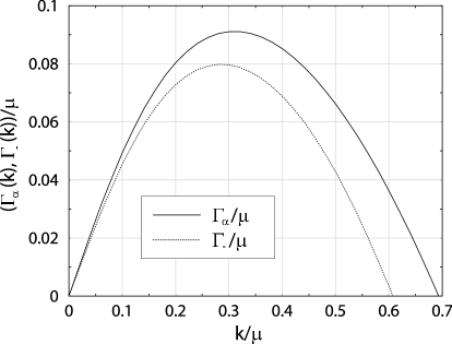
The fact that for $\xi>0$ both $m_{\alpha}^{2}$ and $m_{-}^{2}$ can be negative indicates that the system is unstable to both magnetic and electric fluctuations with the fastest growing modes focused along the beamline ($\theta_{n}=0$). In fact it can be shown that there are two purely imaginary solutions to each of the dispersions relations $\Delta_{\alpha}^{-1}(K)=0$ and $\Delta_{-}^{-1}(K)=0$ with the solutions in the upper half plane corresponding to unstable modes. We can determine the growth rate for these unstable modes by taking $w\rightarrow i\Gamma$ and then solving the resulting dispersion relations for $\Gamma(k)$.

     In Figure 1 I plot the instability growth rates, $\Gamma_{\alpha}$ and $\Gamma_{-}$, as a function of wave number for $\xi=10$ and $\theta_{n}=\pi/8$. Note that both growth rates vanish at $k=0$ and have a maximum $\Gamma_{*}\sim\mu/10$ at $k_{*}\sim\mu/3$. The fact that they have a maximum means that at early times the system will be dominated by unstable modes with spatial frequency $1/k_{*}$.          

Figure 1: Instability growth rates as a function of wave number for $\xi=10$ and $\theta_{n}=\pi/8$.

4 Discretized Hard-Loop Dynamics

It is possible to go beyond an analysis of gluon polarization tensor to a full effective field theory for the soft modes and then solve this numerically. The effective field theory for the soft modes that is generated by integrating out the hard plasma modes at one-loop order and in the approximation that the amplitudes of the soft gauge fields obey $A_{\mu}\ll|\mathbf{p}|/g$ is that of gauge-covariant collisionless Boltzmann-Vlasov equations [22]. In equilibrium, the corresponding (nonlocal) effective action is the so-called hard-thermal-loop effective action which has a simple generalization to plasmas with anisotropic momentum distributions [11]. For the general non-equilibrium situation the resulting equations of motion are

$$D_{\nu}(A)F^{\nu\mu} = -g^{2}\int{d^{3}p\over(2\pi)^{3}}{1\over 2|\mathbf{p}|}\,p^{\mu}\,{\partial f(\mathbf{p})\over\partial p^{\beta}}W^{\beta}(x;\mathbf{v})\,,$$

$$F_{\mu\nu}(A)v^{\nu} = \left[v\cdot D(A)\right]W_{\mu}(x;\mathbf{v})\,,$$ (4)

where $f$ is a weighted sum of the quark and gluon distribution functions [11] and $v^{\mu}\equiv p^{\mu}/|\mathbf{p}|=(1,\mathbf{v})$.

These equations include all hard-loop resummed propagators and vertices and are implicitly gauge covariant. At the expense of introducing a continuous set of auxiliary fields $W_{\beta}(x;\mathbf{v})$ the effective field equations are also local. These equations of motion are then discretized in space-time and ${\mathbf{v}}$, and solved numerically. The discretization in ${\mathbf{v}}$-space corresponds to including only a finite set of the auxiliary fields $W_{\beta}(x;\mathbf{v}_{i})$ with $1\leq i\leq N_{W}$. For details on the precise discretizations used see Refs. [15, 16].

Figure 2: Comparison of the energy transferred from hard to soft scales, $\mid\!\!\mathcal{E}({\rm HL})\!\!\mid$, for 3+1-dimensional simulations with $N_{w}=20,100,200$ on $96^{3},88^{3},69^{3}$ lattices. Inset shows late-time behavior on a linear scale.

4.1 Discussion of Hard-Loop Results

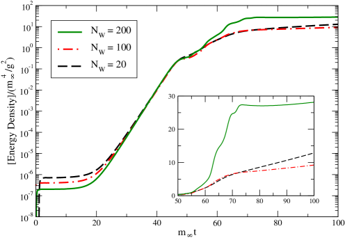
During the process of instability growth the soft gauge fields get the energy for their growth from the hard particles. In an abelian plasma this energy grows exponentially until the energy in the soft field is of the same order of magnitude as the energy remaining in the hard particles. As mentioned above in a non-abelian plasma one must rely on numerical simulations due to the presence of strong gauge field self-interactions. In Fig. 2 I have plotted the time dependence of the energy extracted from the hard particles obtained in a 3+1 dimensional simulation of an anisotropic plasma initialized with very weak random color noise [16]. As can be seen from this figure at $m_{\infty}t\sim 60$ there is a change from exponential to linear growth with the late-time linear slope decreasing as $N_{W}$ is increased.

The first conclusion that can be drawn from this result is that within non-abelian plasmas instabilities will be less efficient at isotropizing the plasma than in abelian plasmas. However, from a theoretical perspective “saturation” at the soft scale implies that one can still apply the hard-loop effective theory self-consistently to understand the behavior of the system at late times. Note, however, that the latest simulations [15, 16] have only presented results for distributions with a finite ${\mathcal{O}}(1\!\!\rightarrow\!\!10)$ anisotropy and these seem to imply that in this case the induced instabilities will not have a significant effect on the hard particles. As a consequence due to the continued expansion of the system the anisotropy will increase. It is therefore important to understand the behavior of the system for more extreme anisotropies. Additionally, it would be very interesting to study the hard-loop dynamics in an expanding system. Naively, one expects this to change the growth from $\exp(\tau)$ to $\exp(\sqrt{\tau})$ at short times but there is no clear expectation of what will happen in the linear regime. Significant advances in this regard have occurred recently [17]. These initial results apply to Abelian plasmas and it would be very interesting to incorporate expansion in collisionless Boltzmann-Vlasov transport in the hard-loop regime and study the late-time behavior in the non-abelian case.

5 Wong-Yang-Mills equations

It is also to possible to go beyond the hard-loop approximation and solve instead the full classical transport equations in three dimensions [21]. The Vlasov transport equation for hard gluons with non-Abelian color charge $q^{a}$ in the collisionless approximation are [23, 24],

$$p^{\mu}[\partial_{\mu}-gq^{a}F^{a}_{\mu\nu}\partial^{\nu}_{p}-gf_{abc}A^{b}_{\mu}q^{c}\partial_{q^{a}}]f(x,p,q)=0~{}.$$ (5)

Here, $f(t,\bf{x},\bf{p},q^{a})$ denotes the single-particle phase space distribution function.

The Vlasov equation is coupled self-consistently to the Yang-Mills equation for the soft gluon fields,

$$D_{\mu}F^{\mu\nu}=J^{\nu}=g\int\frac{d^{3}p}{(2\pi)^{3}}dq\,q\,v^{\nu}f(t,\bf{x},\bf{p},q)~{},$$ (6)

with $v^{\mu}\equiv(1,\bf{p}/p)$. These equations reproduce the “hard thermal loop” effective action near equilibrium [25, 26, 27]. However, the full classical transport theory (5,6) also reproduces some higher $n$-point vertices of the dimensionally reduced effective action for static gluons [28] beyond the hard-loop approximation. The back-reaction of the long-wavelength fields on the hard particles (“bending” of their trajectories) is, of course, taken into account, which is important for understanding particle dynamics in strong fields.

Eq. (5) can be solved numerically by replacing the continuous single-particle distribution $f(\bf{x},\bf{p},q)$ by a large number of test particles:

$$f(\bf{x},\bf{p},q)=\frac{1}{N_{\rm test}}\sum_{i}\delta(\bf{x}-\bf{x}_{i}(t))\,(2\pi)^{3}\delta(\bf{p}-\bf{p}_{i}(t))\,\delta(q^{a}-q_{i}^{a}(t))~{},$$ (7)

where $\bf{x}_{i}(t)$, $\bf{p}_{i}(t)$ and ${q}_{i}^{a}(t)$ are the coordinates of an individual test particle and $N_{\rm test}$ denotes the number of test-particles per physical particle. The Ansatz (7) leads to Wong’s equations [23, 24]

$$\frac{d\bf{x}_{i}}{dt} = \bf{v}_{i},$$ (8)

$$\frac{d\bf{p}_{i}}{dt} = g\,q_{i}^{a}\,\left(\bf{E}^{a}+\bf{v}_{i}\times\bf{B}^{a}\right),$$ (9)

$$\frac{d\bf{q}_{i}}{dt} = ig\,v^{\mu}_{i}\,[A_{\mu},\bf{q}_{i}],$$ (10)

$$J^{a\,\nu} = \frac{g}{N_{\rm test}}\sum_{i}q_{i}^{a}\,v^{\nu}\,\delta(\bf{x}-\bf{x}_{i}(t)).$$ (11)

for the $i$-th test particle. The time evolution of the Yang-Mills field can be followed by the standard Hamiltonian method [29] in $A^{0}=0$ gauge. For details of the numerical implementation used see Ref. [21].

Figure 3: Leftmost figure shows the time evolution of the field energy densities for $SU(2)$ gauge group resulting from a highly anisotropic initial particle momentum distribution. Simulation parameters are $L=5$ fm, $p_{\rm hard}=16$ GeV, $g^{2}\,n_{g}=10/$fm³, $m_{\infty}=0.1$ GeV. Right two panels show the corresponding fourier transforms of the electric and magnetic fields at different times which are indicated in the legend.

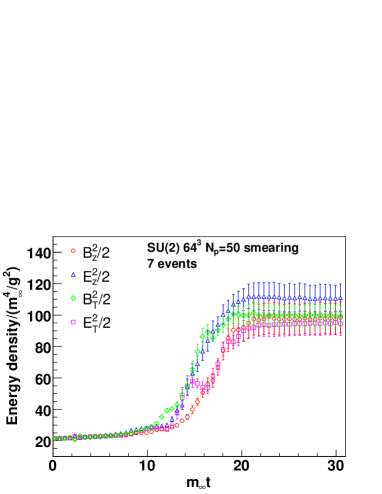
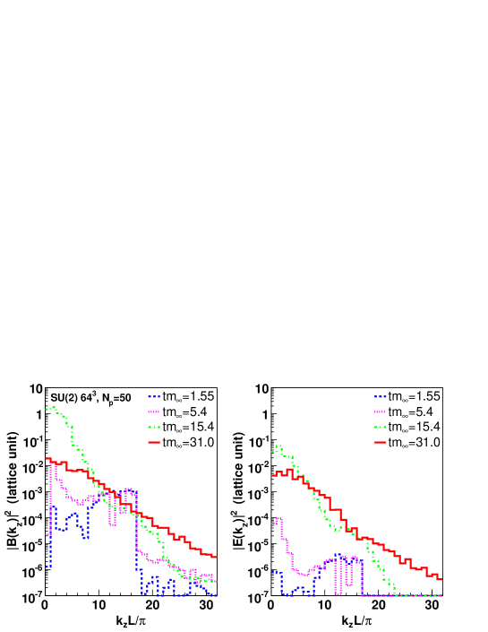
In Fig. 3 I present the results of the three-dimensional simulations published in Ref. [21]. The leftmost panel shows the time evolution of the field energy densities for $SU(2)$ gauge group resulting from a highly anisotropic initial particle momentum distribution. The right two panels show the corresponding fourier transforms of the electric and magnetic fields at different times which are indicated in the legend.

The behavior shown in Fig. 3 indicates that the results obtained from the hard-loop simulations and direct numerical solution of the Wong-Yang-Mills (WYM) equations are qualitatively similar in that both show that for non-abelian gauge theories there is a saturation of the energy transferred to the soft modes by the gauge instability. Additionally, as can be seen from the fourier transforms in right two panels of Fig. 3 the saturation is accompanied by an “avalanche” of energy transferred to soft field modes to higher frequency field modes with saturation occurring when the hardest lattice modes are filled. A more thorough analytic understanding of this ultraviolet avalanche is lacking at this point in time although some advances in this regard have been made recently [30]. Additionally, since within the numerical solution of the WYM equations the ultraviolet modes become populated rapidly this means that the effective theory which relies on a separation between hard (particle) and soft (field) scales breaks down. This should motivate research into numerical methods which can be used to “shuffle” field modes to particles when their momentum becomes too large and vice-versa for hard particles. This is a difficult task but work on such algorithms is in progress. Hopefully, using such methods it will be possible to simulate the non-equilibrium dynamics of anisotropic plasmas in a self-consistent numerical framework which treats particles and fields and the transmutation among these two types of degrees of freedom smoothly.

6 Outlook

An obviously important question is whether quark-gluon plasma instabilities and/or the physics of anisotropic plasmas in general play an important phenomenological role at RHIC or LHC energies. In this regard the recent papers of Refs. [31, 32, 33, 34] provide theoretical frameworks which can be used to calculate the impact of anisotropic momentum-space distributions on observables such as jet shapes and the rapidity dependence of medium-produced photons.

References

- [1] A.H. Mueller, Nucl. Phys. A715 (2003) 20, hep-ph/0208278.
- [2] E. Iancu and R. Venugopalan, (2003), hep-ph/0303204.
- [3] L. McLerran, Nucl. Phys. A752 (2005) 355.
- [4] R. Baier et al., Phys. Lett. B502 (2001) 51, hep-ph/0009237.
- [5] S. Mrowczynski, Phys. Lett. B314 (1993) 118.
- [6] S. Mrowczynski, Phys. Rev. C49 (1994) 2191.
- [7] S. Mrowczynski, Phys. Lett. B393 (1997) 26, hep-ph/9606442.
- [8] P. Romatschke and M. Strickland, Phys. Rev. D68 (2003) 036004, hep-ph/0304092.
- [9] P. Arnold, J. Lenaghan and G.D. Moore, JHEP 08 (2003) 002, hep-ph/0307325.
- [10] P. Romatschke and M. Strickland, Phys. Rev. D70 (2004) 116006, hep-ph/0406188.
- [11] S. Mrowczynski, A. Rebhan and M. Strickland, Phys. Rev. D70 (2004) 025004, hep-ph/0403256.
- [12] P. Romatschke and R. Venugopalan, (2005), hep-ph/0510292.
- [13] P. Romatschke and R. Venugopalan, Phys. Rev. Lett. 96 (2006) 062302, hep-ph/0510121.
- [14] P. Romatschke and R. Venugopalan, (2006), hep-ph/0605045.
- [15] P. Arnold, G.D. Moore and L.G. Yaffe, Phys. Rev. D72 (2005) 054003, hep-ph/0505212.
- [16] A. Rebhan, P. Romatschke and M. Strickland, JHEP 09 (2005) 041, hep-ph/0505261.
- [17] P. Romatschke and A. Rebhan, (2006), hep-ph/0605064.
- [18] P. Arnold and G.D. Moore, Phys. Rev. D73 (2006) 025006, hep-ph/0509206.
- [19] P. Arnold and G.D. Moore, Phys. Rev. D73 (2006) 025013, hep-ph/0509226.
- [20] A. Dumitru and Y. Nara, Phys. Lett. B621 (2005) 89, hep-ph/0503121.
- [21] A. Dumitru, Y. Nara and M. Strickland, (2006), hep-ph/0604149.
- [22] J.P. Blaizot and E. Iancu, Phys. Rept. 359 (2002) 355, hep-ph/0101103.
- [23] S.K. Wong, Nuovo Cim. A65 (1970) 689.
- [24] U.W. Heinz, Phys. Rev. Lett. 51 (1983) 351.
- [25] P.F. Kelly et al., Phys. Rev. Lett. 72 (1994) 3461, hep-ph/9403403.
- [26] P.F. Kelly et al., Phys. Rev. D50 (1994) 4209, hep-ph/9406285.
- [27] J.P. Blaizot and E. Iancu, Nucl. Phys. B557 (1999) 183, hep-ph/9903389.
- [28] M. Laine and C. Manuel, Phys. Rev. D65 (2002) 077902, hep-ph/0111113.
- [29] J. Ambjørn et al., Nucl. Phys. B353 (1991) 346.
- [30] A.H. Mueller, A.I. Shoshi and S.M.H. Wong, (2006), hep-ph/0607136.
- [31] P. Romatschke and M. Strickland, Phys. Rev. D69 (2004) 065005, hep-ph/0309093.
- [32] P. Romatschke and M. Strickland, Phys. Rev. D71 (2005) 125008, hep-ph/0408275.
- [33] B. Schenke and M. Strickland, (2006), hep-ph/0606160.
- [34] P. Romatschke, (2006), hep-ph/0607327.