Discovery and Measurement of Sleptons, Binos, and Winos with a $Z^{\prime}$

Abstract

Extensions of the MSSM could significantly alter its phenomenology at the LHC. We study the case in which the MSSM is extended by an additional $U(1)$ gauge symmetry, which is spontaneously broken at a few TeV. The production cross-section of sleptons is enhanced over that of the MSSM by the process $pp\rightarrow Z^{\prime}\rightarrow\tilde{\ell}\tilde{\ell}^{*}$, so the discovery potential for sleptons is greatly increased. The flavor and charge information in the resulting decay, $\tilde{\ell}\rightarrow\ell+\mbox{LSP}$, provides a useful handle on the identity of the LSP. With the help of the additional kinematical constraint of an on-shell $Z^{\prime}$, we implement a novel method to measure all of the superpartner masses involved in this channel. For certain final states with two invisible particles, one can construct kinematic observables bounded above by parent particle masses. We demonstrate how output from one such observable, $m_{T2}$, can become input to a second, increasing the number of measurements one can make with a single decay chain. The method presented here represents a new class of observables which could have a much wider range of applicability.

1 Introduction

Supersymmetric extensions of the Standard Model, with $M_{\rm soft}\sim 1$ TeV, are probably the most theoretically elegant solutions to stabilize the hierarchy between $M_{P}$ and $\Lambda_{\rm weak}$. The minimal supersymmetric standard model (MSSM) maintains the same gauge symmetries as the Standard Model, while introducing superpartners for the Standard Model particle content. In the past two decades, “standard” experimental signatures of low energy supersymmetry have been carefully studied[1].

The MSSM is the minimal implementation of low energy supersymmetry. However, minimality should not be taken as a fundamental guiding principle in the search for new physics. In fact, the particle content of the SM advocates, if anything, non-minimal physics. In particular, we consider it reasonable to anticipate extensions of the gauge sector as well as the Higgs sector of the MSSM. If the gauge structure or matter content of the MSSM is extended, the phenomenology could be significantly different. There will be novel features deserving attention. New techniques and observables will have to be developed to extract the full information about the underlying model.

Before outlining the main results of our study, we briefly remark on the current status of the study of experimental signatures of the MSSM. As mentioned above, many now classic signatures have been studied[1]. Recently, special attention has been paid to a set of benchmark models[2]. In particular, in SPS1a, it has been shown [3, 4] that mass measurements at the LHC could be achieved to a very high accuracy.

While such studies could be instructive, we remark that the well-studied benchmarks should not be regarded as generic points in the MSSM parameter space. Consequently, the methods of measurements employed probably only have limited applicability and the conclusions could be misleadingly optimistic. In a recent study, [5], it has been shown that there are degeneracies associated with both discrete ambiguities (such as LSP identity) and larger uncertainties (such as slepton masses) in such measurements for a generic point of the MSSM parameter space.

If supersymmetry is discovered at the LHC, one of the biggest challenges will be the study of the properties of the electroweak-inos and the sleptons. In the MSSM, the production of electroweak-inos is usually dominated by the cascade decays of color-charged particles. Such events will typically have a large number of jets, which makes the properties of the electroweak-ino difficult to study. As shown in [5], copious production of leptons in SUSY signals, typically associated with on-shell slepton production and decay, will greatly enhance our ability to study the properties of these superpartners and eliminating degeneracies. The direct production of sleptons $pp\rightarrow Z^{*}/\gamma^{*}\rightarrow\tilde{\ell}\tilde{\ell}^{*}$ that decay to electroweak-inos suffers from a lower rate as well as a large Standard Model background [6, 7]. Although sleptons and electroweak-inos are easy to study in benchmark scenarios such as SPS1a, where $m_{\tilde{q}}>M_{1,2}>m_{\tilde{\ell}}>M_{\rm LSP}$, this is not true generically.

In our study, we consider the LHC phenomenology of extensions of the MSSM, with special focus on its electroweak-ino and slepton sector. For concreteness, we focus on one typical possibility of such an extension, an extra $U(1)^{\prime}$, $m_{Z^{\prime}}\sim{\mathcal{O}}(1)$ TeV, which couples to both quark and lepton supermultiplets. Such an extension is fairly generic as it is present in many GUT/string motivated top-down constructions [8]-[18]. For most of our study, we will consider, as an example, $U(1)_{\rm B-L}$. Being the unique non-anomalous global symmetry of the Standard Model with generation-independent charges, it is perhaps the most likely extension to the gauge sector. We will consider more general possibilities in the discussion of discovery reach. We will demonstrate that the channel $pp\rightarrow Z^{\prime}\rightarrow\tilde{\ell}\tilde{\ell}^{*}$ greatly enhances the discovery reach of $\tilde{\ell}$, and that copiously produced sleptons give an interesting handle on the identity of the LSP. Roughly, this only requires $m_{Z^{\prime}}>2m_{\tilde{\ell}}$. The result of this study is presented in section 2.

Measuring the masses of the superpartners is usually quite difficult, as most of the kinematical observables only measure their mass differences. The unknown momenta of neutral LSP’s lead to undetermined kinematical variables, hindering reconstruction of the event. Guesses of unknown variables are usually unreliable since there are several of them. Such a difficulty is expected to persist in the $pp\rightarrow Z^{*}/\gamma^{*}\rightarrow\tilde{\ell}\tilde{\ell}^{*}$ channel, which has 3 unknown variables. The existence of an on-shell $Z^{\prime}$ provides one additional kinematical constraint and should enable us to do better. One of the main results of this paper is the development of a new method which fully takes advantage of such a constraint. This allows us to completely determine the slepton mass and the LSP mass with properly chosen observables. Our method is presented in section 4.

For most of this study we will assume for simplicity that the sleptons are degenerate in mass. We remark that we should expect a certain amount of splitting between the left-handed and right-handed sleptons, at least from the effect of RGE running from a high scale. Such effects are more prominent if the overall mass scale of the sleptons is low. In models such as gauge mediation where there is a significant contribution from a $Z^{\prime}_{B-L}$, [19] we expect a larger universal contribution to both left-handed and right-handed sleptons. Nevertheless, we emphasize that the effect of left-right splitting is important and deserves further study. A detailed consideration of this issue is outside the scope of this paper. The methods we introduce for mass measurement could be modified, possibly by introducing additional observables, in order to deal with this further complication. In the conclusion of this paper, we will further argue that this effect does not impact the discovery reach as long as $Z^{\prime}$ decays into both left and right sleptons are still allowed. If one of them becomes heavier than $m_{Z^{\prime}}/2$ however, the signal significance should drop accordingly.

In our study, events are generated at the matrix element level using COMPHEP-4.4.3 [20] and piped through PYTHIA 6.3 [21] for initial state radiation and hadronization. PGS[22] is used as detector simulation.

In section 2, we investigate the reach at the LHC for sleptons in models with an extended gauge sector and compare it to the MSSM for certain benchmark scenarios. We show how to use the $Z^{\prime}$ to determine the LSP identity in section 3. In section 4, we discuss mass measurements for these benchmark scenarios.

2 Discovery

In this section and for most of this the paper we concentrate on the production channel

$$pp\rightarrow Z^{\prime}\rightarrow\tilde{\ell}~{}\tilde{\ell}^{*}\rightarrow\ell^{+}~{}\ell^{-}+\not{E}_{T}$$ (1)

where $\tilde{\ell}$ can be a sneutrino as well as a charged slepton. We also include the MSSM process

$$pp\rightarrow Z^{*}/\gamma^{*}\rightarrow\tilde{\ell}~{}\tilde{\ell}^{*}\rightarrow\ell^{+}~{}\ell^{-}+\not{E}_{T}$$ (2)

for comparison.

In general, we consider an extra $U(1)_{B-xL}$, which couples to the SM fermions through

$$\mathcal{L}\supset g\ \bar{\psi}\ q_{B-xL}\ \gamma^{\mu}Z_{\mu}\ \psi,$$ (3)

where $q_{B-xL}$ is the charge of the SM fermions under $U(1)_{B-xL}$.

In the MSSM, the $Z^{*}/\gamma^{*}$ mediated slepton pair production cross section falls sharply with $\hat{s}\geq 4m_{\tilde{\ell}}^{2}$, and therefore with increasing slepton mass. On the other hand, for $m_{\tilde{\ell}}<m_{Z^{\prime}}/2$, the production through $Z^{\prime}$ resonance is almost independent of $m_{\tilde{\ell}}$, up to a very mild phase-space factor, leading to a great enhancement in the discovery reach. In figure 1 we display the improvement of the charged slepton (one flavor) production cross section over the MSSM for our benchmark scenario, with a $Z^{\prime}_{B-L}$ at 2.0 TeV and $g_{B-L}=0.25$.

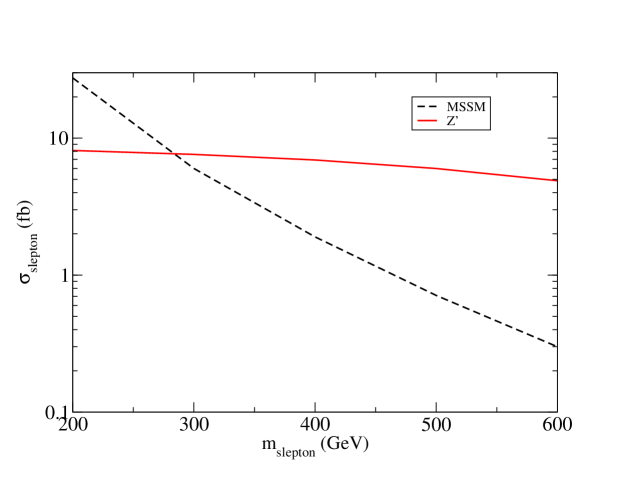
Figure 1: The cross section for one flavor of charged slepton pair production in the MSSM (dashed curve) and our benchmark scenario with a $Z^{\prime}_{B-L}$ at 2 TeV and $g_{B-L}=0.25$ (solid curve).

In our analysis we preselect events with an opposite sign same flavor dilepton pair and use a jet veto (where jets are identified using a cone algorithm with R=0.7 and a $p_{T}$ cut of 10 GeV). This significantly reduces SM background at high $p_{T}^{\ell}$. In our background analysis, we include W/Z pair production generated by PYTHIA, and in the case that the final state lepton is an electron we consider the effect of $W+j\rightarrow\rm{fake}~{}e^{+}e^{-}$ (which we find to be negligible). The background analysis assumes $\sqrt{N}$ statistics, which allows us to find a rough estimate for the slepton reach at the $5\sigma$ level. We use data samples of $100~{}\rm{fb}^{-1}$.

In the preselected events we consider two observables, the $\not{E}_{T}$ of the event and the $p_{T}$ of the softer lepton. As expected, we find that with these choices signal can generically be distinguished from background with relative ease by cutting on either of those observables. This is demonstrated in figure 2. We also include the MSSM case for comparison and see that it is difficult to separate from the background. Direct production in the MSSM was studied in detail in [6, 7].

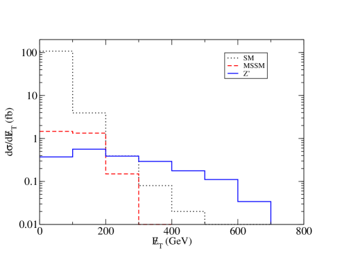
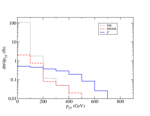
Figure 2: Preselecting final state signatures of a same flavor opposite sign dilepton pair using a jet veto, comparison of the differential cross section for $\not{E}_{T}$ (above) and the softer lepton $p_{T}$ (below) in background, MSSM direct production and $Z^{\prime}$ resonant production in our benchmark scenario with $m_{\tilde{\ell}}=200~{}\rm{GeV}$ and $m_{LSP}=100~{}\rm{GeV}$.

2.1 LHC reach for sleptons in the MSSM

In the MSSM, the available decay modes of sleptons depend on the identity of the LSP, and are especially sensitive to whether there is a chargino nearly degenerate in mass with the LSP. Therefore, we study the discovery reach in several different scenarios with different LSP’s. We discuss briefly the reach in the MSSM for each scenario in this section.

Our first scenario (I) has a bino LSP, with MSSM parameters given by Table 1. Sleptons are produced solely through $pp\rightarrow Z^{*}/\gamma^{*}\rightarrow\tilde{\ell}~{}\tilde{\ell}^{*}$ and they decay to the LSP. Sneutrinos do not play a role in this scenario. For a single flavor (taken to be $e$) we find that the slepton discovery reach at $5\sigma$ is $m_{\tilde{\ell}}\leq 300$ GeV.

Our next scenario (II) has a wino LSP. In this case, the left handed sleptons can decay to $\chi_{1}^{\pm}$ thereby reducing the number of dilepton events compared to (I), while right handed sleptons can only decay through the effects of gaugino and higgsino mixing. The sneutrinos also produce dileptons as they decay to $\chi_{1}^{\pm}$. We find that the $5\sigma$ discovery reach is $m_{\tilde{l}}\leq 175$ GeV. The pattern of the leptonic signatures in this scenario is quite interesting, which we will discuss in detail in the next section.

We also include a scenario (III) with a higgsino LSP which will be of interest when we attempt to determine the identity of the LSP in the following sections.

name	$M_{1}$	$M_{2}$	$\mu$	$\tan{\beta}$
I	$100$ GeV	$2$ TeV	$2$ TeV	10
II	$2$ TeV	$100$ GeV	$2$ TeV	10
III	$2$ TeV	$2$ TeV	$100$ GeV	10

Table 1: The MSSM input parameters for the scenarios we consider. We decouple additional states by raising their mass above the squark and slepton masses.

In order to demonstrate our signatures in cases with straightforward physics interpretations, we have chosen non-LSP electroweak-ino mass parameters so that the identity of the lightest electroweak-inos are pure gauge eigenstates and mixings induced by electroweak symmetry breaking are negligible. We have in fact studied scenarios where the electroweak-inos are split much more moderately, $m_{\rm non-LSP}\gtrsim 800$ GeV, and found that our results in the next few sections are virtually unaffected.

2.2 MSSM$+U(1)_{B-xL}$ Scenarios

Taking into account the mass and coupling bounds from LEP [23, 24] and from the Tevatron [25] in $U(1)_{B-xL}$ scenarios, we will only be interested in models where $\frac{m_{Z^{\prime}}}{g}\gtrsim x\ (6~{}\rm{TeV})$.

In a general study of $U(1)_{B-xL}$, we consider the spectrum of scenario I, with sleptons at $400$ GeV and the $Z^{\prime}$ at $2.0$ TeV, and vary both $x$ and the coupling strength $g$. In figure 3 we display the $5\sigma$ discovery contour at $100~{}\rm{fb}^{-1}$, our benchmark point and the exclusion contour from LEP data for this choice of $Z^{\prime}$ mass. At very small $g$, not enough $Z^{\prime}$s are produced to overcome background and at very small $x$ the branching ratio of $Z^{\prime}\rightarrow\ell\bar{\ell}$ is too small so $g$ has to be rather large for discovery.

Figure 3: In a scenario with $m_{\tilde{\ell}}=400~{}\rm{GeV}$ and $m_{Z^{\prime}}=2.0~{}\rm{TeV}$ where the $U(1)$ couples to baryon number with strength $g$ and to lepton number with strength $xg$, one flavor of sleptons can be discovered at the $5\sigma$ level at $100~{}\rm{fb}^{-1}$ in the region to the upper right of the solid curve in the $g-x$ plane. LEP data excludes anything to the upper right of the dashed curve. Our benchmark point is indicated by the solid dot. If we increase the mass of the $Z^{\prime}$, both the reach curve and the LEP constraint will shift upward and to the right.

Next, we study the reach of slepton discovery as a function of the $Z^{\prime}$ mass, which is one of the most important factors determining the rate and hence the reach. For concreteness, we couple to scenarios I and II a $U(1)_{B-L}$ with $g=0.25$ (and, naturally, $x=1$). We scan over the mass of the $Z^{\prime}_{B-L}$ and find a great improvement in the reach for sleptons at $5\sigma$ over the MSSM. Our results are displayed in figure 4. At relatively low $m_{Z^{\prime}}$, we find that sleptons can be discovered in most of the kinematically allowed region $m_{\tilde{\ell}}\leq m_{Z^{\prime}}/2$. Heavier $m_{Z^{\prime}}$ are rarely produced, and so one needs enough phase space to win over background. Therefore, the sleptons have to be light enough to be produced far from the kinematic threshold.

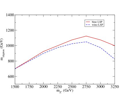
Figure 4: In bino LSP scenario and wino LSP scenario, we display the $5\sigma$ slepton discovery reach at the LHC at $100~{}\rm{fb}^{-1}$ in the presence of a $U(1)_{B-L}$ with $g=0.25$ and $x=1$ as a function of the $Z^{\prime}$ mass. For comparison, in the MSSM, the reach is $m_{\tilde{\ell}}\leq 300~{}\rm{GeV}$ in bino LSP scenario and $m_{\tilde{\ell}}\leq 175~{}\rm{GeV}$ in wino LSP scenario.

3 Identity of the LSP

In this section, we investigate the possibility of using the lepton information of the leptons from $Z^{\prime}$ decay to study the identity of the LSP.

Depending on details of the mass spectrum, it is possible to study the identities of the light electroweak-inos by studying soft jets or the possible existence of displaced vertices in cascade decays involving nearly degenerate electroweak-ino states [26, 27]. The electroweak-ino can have a decay chain with large branching fraction into isolated, energetic leptons. These carry charge and flavor information and also provide a very powerful clean experimental probe to the identities of the electroweak-inos. In the MSSM, the best channel for such a study is $\chi^{0}_{2}\rightarrow\tilde{\ell}~{}\ell\rightarrow\ell^{+}~{}\ell^{-}~{}\chi^{0}_{1}$. However, as commented in the introduction, we should not regard this as a typical channel as it requires a certain arrangement of the spectrum. In our case, copiously produced sleptons from the $Z^{\prime}$ decay and $\tilde{\ell}\rightarrow\ell~{}\chi^{0}_{1}$ will carry additional important information and provide a further handle on the LSP identity.

In the following analysis we will be interested in the ratio of opposite sign dilepton events to single lepton events with a jet veto, restricting ourselves to one flavor ($e^{\pm}$) as before. As we have already seen, in the case of a $U(1)_{B-L}$, the dilepton signal dominates over SM background at high $p_{T}$. The single lepton signal has a larger background from singly produced $W^{\pm}$ bosons but using a jet veto and concentrating on high $p_{T}$ events still leaves us with a statistically significant excess, as we will show later in this section.

	$R_{(\ell^{+}\ell^{-})/(1\ell)}$	gaugino content
bino LSP	$>100$	$V_{\chi_{1}^{0},\tilde{W}}=2.28\times 10^{-4}$, $V_{\chi_{1}^{0},\tilde{B}}=-0.9998$
wino LSP	$1.4$	$V_{\chi_{1}^{0},\tilde{W}}=0.999$ $V_{\chi_{1}^{0},\tilde{B}}=-2.28\times 10^{-4}$
		$V_{\chi_{1}^{\pm},\tilde{W}}=-0.99996$ $U_{\chi_{1}^{\pm},\tilde{W}}=-0.998$
higgsino LSP	$3.3$	$V_{\chi_{1}^{0},\tilde{W}}=0.032$ $V_{\chi_{1}^{0},\tilde{B}}=-0.018$
		$V_{\chi_{2}^{0},\tilde{W}}=0.024$ $V_{\chi_{2}^{0},\tilde{B}}=-0.013$
		$V_{\chi_{1}^{\pm},\tilde{W}}=-0.057$ $U_{\chi_{1}^{\pm},\tilde{W}}=-0.008$

Table 2: The correlation between the electroweak-ino mixing and the ratio of dilepton events to single lepton events in the three scenarios we consider with $m_{\tilde{\ell}}=400~{}\rm{GeV}$ for $100~{}\rm{fb}^{-1}$ of data. The ratio has been obtained for pure signal but includes detector effects. $V_{\chi_{1}^{0},\tilde{w}}$ etc. denote the relevant entries in the electroweak-ino mixing matrix.

The characteristics of the leptonic signature from the decay $\tilde{\ell}\rightarrow\ell+\mbox{LSP}$ depend mostly on the bino and wino content of the LSP. A mostly bino LSP has the very distinctive feature that dilepton events greatly dominate over single lepton events, as charged sleptons always decay to $\chi_{1}^{0}$ via charged leptons. Any observed single lepton events with this process are due to detector effects. This can be seen in our example scenario I, as shown in Table 2. On the other hand, a wino LSP will offer the roughly comparable possibility of both dilepton and single lepton signatures. The slepton decaying directly into neutral wino LSP will produce only dilepton signature, just like the bino LSP case. On the other hand, there is a charged wino state which is usually nearly degenerate with the LSP. Since it is very difficult to detect the existence of the process $\tilde{\chi}^{\pm}\rightarrow\tilde{\chi}^{0}+\mbox{soft particles}$, we can effectively treat the chargino as the end of the visible decay chain. Slepton decaying processes $\tilde{\ell}^{+}\tilde{\ell}^{-}\rightarrow\ell^{\pm}+\tilde{\chi}^{\mp}+\nu+\tilde{\chi}^{0}$ and $\tilde{\nu}\tilde{\nu}^{*}\rightarrow\ell^{\pm}+\tilde{\chi}^{\mp}+\nu+\tilde{\chi}^{0}$ will give rise to single lepton signatures, while $\tilde{\nu}\tilde{\nu}^{*}\rightarrow\ell^{\pm}+\tilde{\chi}^{\mp}+\ell^{\pm}+\tilde{\chi}^{\mp}$ can give rise to additional opposite sign dilepton signatures. Therefore, the ratio

$$R_{(\ell^{+}\ell^{-})/(1\ell)}=\frac{\#\mbox{ of OS dilepton events}}{\#\ \mbox{of 1 lepton events}},$$ (4)

should give us a very clear handle distinguishing the wino and bino LSP cases, as shown in Table 2.

The higgsino LSP case is more intricate. Since the Yukawa coupling of electrons is negligible, observables depend solely on bino/wino components of the lightest neutralino, as well as the wino component of the charged higgsinos, making the higgsino LSP scenario more difficult to distinguish from the other cases. In fact, we find the dilepton to single lepton ratio in our scenario III to be closer to the wino case ($\sim 1:1$) than the bino case ($>100:1$), as can be seen in table 2. If the gaugino/higgsino masses are changed, the amount of mixing will be affected and the signatures of scenario III can vary between the extreme cases of scenarios I and II.

Having established an important difference between scenarios with different LSP identities, we discuss the possibility of distinguishing these scenarios in the presence of background. For signal with single lepton, we use a background sample of diboson and single $W^{\pm}$ production and look for events with a single very high-$p_{T}$ electron in the absence of jets. While we consider MSSM background as well, we find that after cuts its contribution is negligible. We study the single lepton production rate and find an excess over background of $4.2\sigma$ in our scenario II and $2.4\sigma$ in scenario III for $100~{}fb^{-1}$ of integrated luminosity where the statistical significance of the excess lies in the region $p_{T}>500~{}\rm{GeV}$. Not surprisingly, scenario I does not give rise to any excess in single-lepton events so the higgsino LSP case lies roughly in the middle of the pure wino and bino cases.

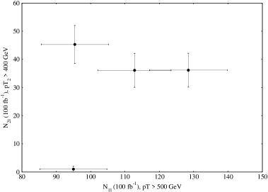
Figure 5: The number of dilepton ($p_{T2}>400~{}\rm{GeV}$) and single lepton ($p_{T}>500~{}\rm{GeV}$) events with a jet veto in $100~{}\rm{fb}^{-1}$ of data. The background is given by the point close to the x-axis while the points away from the x-axis represent (from left to right) scenarios I, III and II respectively. The sizes of the error bars denote $1\sigma$ using $\sqrt{N}$ statistics, which include both the signal and the background.

While the signal-only ratios in table 2 become much more uncertain due to background, we illustrate in figure 5 that scenarios I and II can still be distinguished due to the combined observability of single lepton and dilepton events, where using a jet veto we count single lepton events with $p_{T}>500~{}\rm{GeV}$ and dilepton events where the softer lepton has $p_{T}>400~{}\rm{GeV}$ in $100~{}\rm{fb}^{-1}$ of data. With $100$ fb^-1 of data, scenario III is not clearly distinguishable from scenario II. In fact, as we remarked earlier, the higgsino LSP case is expected to interpolate between the bino and wino LSP cases as the gaugino content of the LSP varies between being bino-like and wino-like, while the coupling of the higgsino to electrons is irrelevant.

While we have not taken advantage of them in our analysis, there are other potential differences between signal and background, such as the charge asymmetry in single lepton events from $W^{\pm}$ production due to the pp-initial state which is absent in $Z^{\prime}$ initiated events. Exploring such effects fully can enhance the signal to background ratio in a more complete analysis.

We mention here one additional example of the sensitivity of leptonic signatures to the structure of the electroweak-ino sector. One can have an $e$-$\mu$ non-universality coming purely from gaugino-higgsino mixing. In our scenario II, we find that for $\tilde{\mu}_{R}$, which does not couple to the wino, the Yukawa coupling is just large enough for the branching ratio to $\chi_{1}^{\pm}$ to be greatly enhanced through higgsino mixing while $\tilde{e}_{R}$ decays exclusively to $\chi_{1}^{0}$ through its bino component. This is an interesting source of $e/\mu$ asymmetry that merits further study, but for us this just means that $e^{+}e^{-}$ is a better final state to consider than $\mu^{+}\mu^{-}$.

In summary, we see that the leptonic signature provides a very strong handle on the identity of the LSP. The higgsino LSP case or longer decay chains with more electroweak-inos could still give degeneracies but we expect a dramatic decrease in such degeneracies compared to the general MSSM. This agrees with the observation made in [5] in the case of on-shell sleptons. Since $Z^{\prime}$s generically give us a new source of on-shell sleptons, they help improve our ability to untangle the electroweak-ino sector.

4 Measurements of Masses

As argued above, in MSSM scenarios it is not generic for sleptons to be produced on shell copiously, and even if discovery is possible, one does not necessarily have enough statistics for mass measurements. In this section we will look in more detail into certain measurements made possible by the presence of a spontaneously broken $U(1)$.

Figure 6: Momentum labeling conventions for Section 4.

4.1 General considerations

In this section, we consider the case where the end of the SUSY decay chain is a stable electroweak-ino. For concreteness, we focus on the bino-LSP scenario. Due to the generic nature of the method we present here, we expect that it is straightforwardly applicable to other identities of the electroweak-ino LSPs. We will begin by reviewing the property of a set of generic $p_{T}$-like observables, using $m_{T2}$ as an example.

The $m_{T2}$ variable, as developed in [28, 29, 30, 31], offers a straightforward way to calculate slepton mass in certain two-body decays. In our case, sleptons are pair-produced by the $Z^{\prime}$ with $\tilde{\ell}\rightarrow\ell+\tilde{\chi}$ processes on either side of the decay as in figure 6. By properly combining the lepton and missing energy information with the value of $m_{\chi_{1}}$, one can measure $m_{\tilde{\ell}}$.

To construct $m_{T2}$, the unknown momenta $q_{1}$, $q_{2}$ of the two $\tilde{\chi}$’s are assigned in every way that satisfies the missing energy constraint $\mathbf{q}_{1T}+\mathbf{q}_{2T}=\not{\mathbf{p}}_{T}$. For each assignment of momenta, one constructs the transverse mass squared for both halves of the decay,

$$m_{T}^{2}(\mathbf{p}_{1T},\mathbf{q}_{1T},m_{\chi_{1}})=m_{\ell}^{2}+m_{\chi_{1}}^{2}+2(E_{T}^{\ell}E_{T}^{\chi}-\mathbf{p}_{1T}\cdot\mathbf{q}_{1T})$$

where $E_{T}=\sqrt{\bf{p}_{T}^{2}+m^{2}}$. Since the transverse mass satisfies $m_{T}<m_{\tilde{\ell}}$, the branch with a greater $m_{T}^{2}$ gives a tighter constraint on $m_{\tilde{\ell}}$. Taking the greater of the two $m_{T}^{2}$’s and minimizing this quantity over all possible assignments of $q_{1}$ and $q_{2}$ gives $m_{T2}$ for the event. This is by construction less than the true transverse mass for one branch of the decay, which is in turn less than the mass of the parent particle, in our case $m_{\tilde{\ell}}$. Thus, the distribution of $m_{T2}$ for all events has an endpoint at $m_{\tilde{\ell}}$.

The same information could be extracted from $p_{T}$ distributions of the visible particles. Very roughly, we expect the lepton $p_{T}$ distribution to peak near $m_{\tilde{\ell}}-m_{\chi_{1}}$. In principle, we could make this statement quantitative by simulating the decay process for various input masses and fitting to the resulting $p_{T}$ distributions. The $m_{T2}$ endpoint does not carry more statistical weight than such a fit, but it has the practical advantage that it gives a quantitative measurement with a simple interpretation that does not require fitting to simulated data.

To compute $m_{T2}$ and reliably interpret its endpoint as the slepton mass, we must already know the LSP mass $m_{\chi_{1}}$. When $m_{\chi_{1}}$ is unknown, a free input mass $M_{\rm{guess}}$ takes its place in the $m_{T2}$ equation:

$$m_{T2}^{2}(M_{\rm{guess}})\equiv\min_{\mathbf{q}_{1T}+\mathbf{q}_{2T}=\not{\mathbf{p}}_{T}}\left[\max\left\{m_{T}^{2}\left(\mathbf{p}_{1T},\mathbf{q}_{1T};M_{\rm{guess}}\right),m_{T}^{2}\left(\mathbf{p}_{2T},\mathbf{q}_{2T};M_{\rm{guess}}\right)\right\}\right]$$ (5)

We use a $130~{}\rm{fb}^{-1}$ sample of selectron and smuon pair production (opposite sign same flavor dileptons, $\not{E}_{T}$, no jets or photons harder than 20 GeV) with $M_{1}=100$ GeV and $M_{\tilde{\ell}}=400$ GeV. Knowing $m_{\chi_{1}}$ to be 100 GeV, and plotting the distribution of $m_{T2}$, we find the endpoint with a linear fit and measure $m_{\tilde{\ell}}=405$ GeV (see figure 7).

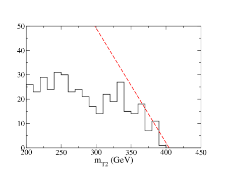
Figure 7: $m_{T2}$ for $\tilde{\ell}\rightarrow\ell+\tilde{\chi}_{1}$ with 130 $\rm{fb}^{-1}$. Endpoint at 405 GeV. ($m_{\chi_{1}}=100$ GeV, $m_{\tilde{\ell}}=400$ GeV)

In the scenario where we know $m_{\chi_{1}}$ from another measurement, $m_{T2}$ allows a quick and accurate determination of $m_{\tilde{\ell}}$ [28, 30], even if we ignore the on shell $Z^{\prime}$ at the top of the decay. If $m_{\chi_{1}}$ is unknown, then the $m_{T2}$ endpoint gives one constraint for the two unknown masses $m_{\chi_{1}}$ and $m_{\tilde{\ell}}$, but it is not clear how to interpret it. The endpoint does not fall at either the slepton mass or the mass difference, and it does not vary linearly with the input mass, $M_{\rm{guess}}$. As we will show below, the presence of the $Z^{\prime}$ allows one to use $m_{T2}$ without this extra piece of knowledge. That is, we can measure both $m_{\tilde{\ell}}$ and $m_{\chi_{1}}$ at the same time. To this end, we present a technique that determines $m_{\chi_{1}}$ to within 15 GeV.

To understand how $m_{T2}$ varies as a function of the unknown LSP mass $M_{\rm{guess}}$, we generated a sample of unreasonable luminosity, $7~{}\rm{ab}^{-1}$ (100,000 events), and calculated $m_{T2}$ for a wide range of input masses. One might hope that $m_{T2}$ would change linearly as $M_{\rm{guess}}$ is varied, but this only holds in the limit of large input mass, asymptoting to a line of slope 1. This matches the behavior found in [31]. Figure 8 shows how the accuracy in determining $m_{\tilde{\ell}}$ depends on the uncertainty in $m_{\chi_{1}}$. The discrepancy between $m_{T2}$ at the correct value of $M_{\rm{guess}}$ and $m_{\tilde{\ell}}$ is a systematic effect due to radiation and detector resolution and is independent of luminosity.

Figure 8: $m_{T2_{\rm endpoint}}$ for vs. $M_{\rm{guess}}$ for $m_{\chi_{1}}=100$ GeV. 100,000 events.

Thus, in the generic $m_{T2}$ scenario, without outside of knowledge of $m_{\tilde{\ell}}$ or $m_{\chi_{1}}$, one obtains a curve in $m_{\tilde{\ell}}$-$m_{\chi_{1}}$ space. With the extra constraint offered by a $Z^{\prime}$, one might hope to reduce the uncertainty in $m_{\chi_{1}}$, collapsing the curve to a much smaller region. In this case, we have

$$8_{q_{1,2}}-2_{\not{p}_{T}}-1_{m_{{\rm LSP}_{1}}=m_{{\rm LSP}_{2}}}-1_{m_{\tilde{\ell}_{1}}=m_{\tilde{\ell}_{2}}}-1_{m_{Z^{\prime}}}-1_{m_{T2_{\rm endpoint}}}=2\ \mbox{unknowns}.$$ (6)

In a situation without a $Z^{\prime}$, we would have three unknowns, which we could take to be $q^{x,y}_{\chi_{1}}$ and $m_{\chi_{1}}$. Given values for these unknowns, we could reconstruct the event up to a fourfold algebraic ambiguity from solving a quadratic equation for $q^{z}_{\chi}$ for each half of the event. In the presence of the $Z^{\prime}$, however, we have a constraint on the total four-momentum. With a properly sensitive quantity, one could hope to show that only in a small region of $m_{\tilde{\ell}}$-$m_{\chi_{1}}$ space does one sensibly reconstruct the $Z^{\prime}$ at its predetermined mass.

In general, one could employ two strategies to achieve this. First, we could make some kinematical guesses about the unknowns and try to reconstruct the kinematics. As mentioned above, for any event there is the following hierarchy: $m_{T2}<m_{T}<m_{\tilde{\ell}}$, where $m_{T}$ is the actual transverse mass of one branch of the event. For values of $m_{T2}$ near the endpoint, one has approximately the correct $m_{T}$, so one might hope that the reconstructed LSP momenta are also approximately correct. This will be true provided that only a small region of LSP momenta is physically allowed after constraining $m_{\tilde{\ell}}=m_{T2_{\rm endpoint}}$. Attempts to measure the bino mass with this technique, taking the 10$\%$ of events with $m_{T2}$ closest to the $m_{T2}$ endpoint, were accurate to within only 100 GeV for 130 $\rm fb^{-1}$. As shown in figure 9, the LSP momenta we reconstruct with this method only correlate roughly with the Monte Carlo truth, limiting the accuracy of this technique. As a second approach, we could take all possible values of the unknown variables and try to construct some observable which is bounded by the true values for the unknown variables. We will present a method based on this latter strategy. It works considerably better than the first, measuring the bino to within 15 GeV for 130 $\rm fb^{-1}$.

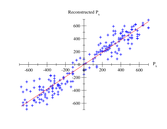
Figure 9: Comparison of the actual $p_{x}$ of the LSP to the $p_{x}$ as reconstructed using the top tenth of events closest to the $m_{T2}$ endpoint.

4.2 Constructing an Endpoint at $m_{Z^{\prime}}$

The basic approach is to use $m_{T2}$ to compute $m_{\tilde{\ell}}$ as a function of $M_{\rm{guess}}$, and then to impose another constraint by demanding that the initial $Z^{\prime}$ be on shell. A step-by-step outline of our approach is as follows:

1. Measure the $Z^{\prime}$ mass in an unrelated channel, such as $Z^{\prime}\rightarrow e^{+}e^{-}$.

2. Guess $M_{\rm{guess}}$, the mass of the LSP.

3. Use $m_{T2}(M_{\rm{guess}})$ to compute the slepton mass.

4. Compute the $Z^{\prime}$ mass. This is done by reconstructing every event in every possible way, picking the minimum allowed $Z^{\prime}$ mass for each event, then maximizing this minimum over all events.

5. Compare the $Z^{\prime}$ mass computed in step 4 to the actual $Z^{\prime}$ mass measured in step 1. If the answers are inconsistent, throw out this guess for the LSP mass $M_{\rm{guess}}$.

6. Repeat this process for a range of LSP masses $M_{\rm{guess}}$.

The definition of $m_{T2}$, eq.(5), implies a “max-min” approach that can be applied very generally to processes with invisible final state particles: Given some unknown, $M$, construct an observable that is bounded above by the true value of $M$. Minimize the observable over all unknowns in each event, and plot the result for all events. The resulting distribution has an endpoint at the true value of $M$. This process can be applied sequentially, using the result of the first application as an input to the second. As an example, we first apply $m_{T2}$ to compute $m_{\tilde{\ell}}(M_{\rm{guess}})$, then apply the strategy again to compute $m_{Z^{\prime}}$. This gives us a measurement of one of the masses $m_{\chi},m_{Z^{\prime}}$ if the other mass is known from another channel.

The computation of $m_{T2}$ was described above. For given values of the unknown momenta $q_{1},q_{2}$ that are physically sensible (i.e. satisfy $m_{T}<m_{\tilde{\ell}}$), we then use the slepton mass constraint (setting $m_{\tilde{\ell}}=m_{T2_{\rm endpoint}}$) to reconstruct $m_{Z^{\prime}}$. Again, there is a fourfold ambiguity in $m_{Z^{\prime}}$ resulting from the solutions to the two quadratic equations that determine $q^{z}_{1,2}$. For each event, define the observable

$$m_{Z^{\prime}}^{\rm{min}}=\min_{q_{1},q_{2}}\left(\min_{\rm{4\,choices}}(m_{Z^{\prime}}(q_{1},q_{2}))\right)$$ (7)

where the inner minimum is taken over the fourfold ambiguity, and the outer minimum is taken over all values of LSP momenta $q_{1}$ and $q_{2}$ that reproduce the correct missing energy and obey $m_{T}<m_{T2_{\rm endpoint}}$. This observable clearly satisfies $m_{Z^{\prime}}^{\rm{min}}<m_{Z^{\prime}}$. Taken over many events, $m_{Z^{\prime}}^{\rm{min}}$ has an endpoint at the actual $Z^{\prime}$ mass (or, more accurately, at $m_{Z^{\prime}}+\Gamma_{Z^{\prime}}$) . Detector resolution, finite width of the $Z^{\prime}$, and the coarseness of our momentum sampling grid will smear the result. However, we nonetheless get an $m_{T2}$-like endpoint at the upper end of the $Z^{\prime}$ width. In the end, we are not actually interested in measuring $m_{Z^{\prime}}$, because it can be measured directly in another channel such as $Z^{\prime}\rightarrow\ell^{+}\ell^{-}$. Instead, we use $m_{Z^{\prime}}$ as an additional constraint to determine the LSP mass $m_{\chi_{1}}$.

We performed our analysis on an integrated luminosity of $130~{}\rm{fb}^{-1}$ for $M_{1}=100$ and $M_{1}=250$ GeV. The $Z^{\prime}$ has mass $m_{Z^{\prime}}=2$ TeV and width $\Gamma_{Z^{\prime}}=27$ GeV. The $m_{Z^{\prime}}^{\rm{min}}$ endpoints are shown in figure 10 for the correct input masses for $M_{\rm{guess}}$. We plot the value of the $m_{Z^{\prime}}^{\rm{min}}$ endpoint as a function of input mass for the two cases in figure 11. The uncertainty from the endpoint-fitting algorithm and Monte Carlo simulation (determined by repeating the analysis 15 times with different random number seeds) is 27 GeV. There is an additional source of uncertainty we did not estimate, which is the expected position of the $m_{Z^{\prime}}^{\rm{min}}$ endpoint. In both scenarios we examined, this fell near the endpoint of the $Z^{\prime}$ width, $m_{Z^{\prime}}+\Gamma_{Z^{\prime}}$ = 2.027 TeV, but there is no reason to expect this to be exact. A determination of this uncertainty may loosen the bound we set, but we do not expect it to do so significantly. For both cases, over a range of a few hundred GeV, we sampled $M_{\rm{guess}}$ at 10 GeV intervals. In the $M_{1}=100$ scenario, only for the correct guess mass of 100 GeV and 90 GeV did $m_{Z^{\prime}}+\Gamma_{Z^{\prime}}$ fall within the statistical uncertainty. For the $M_{1}=250$ case, only the correct 250 GeV guess mass had $m_{Z^{\prime}}+\Gamma_{Z^{\prime}}$ in its uncertainty. These results are summarized in Table 3. In both cases we can determine the bino mass to within 15 GeV. An improved understanding of detector resolution effects could allow an even tighter bound.

Finally, this can be compared to the original $m_{T2}(M_{\rm{guess}})$ values to determine the slepton mass as well. For $m_{\chi_{1}}=100$ GeV we find $m_{\tilde{\ell}}=405$ with an uncertainty $<\pm 10$ GeV, and for $m_{\chi_{1}}=250$ GeV we find $m_{\tilde{\ell}}=407$ GeV with an uncertainty $<\pm 15$ GeV. These uncertainties include only the 27 GeV uncertainty mentioned above. We did not include the uncertainty in measuring the $m_{T2}$ endpoint.

To determine the robustness of the analysis in the limit of low statistics, we compared uncertainties for $M_{\rm{guess}}=100$ in the $m_{\chi_{1}}=100$ case (figure 11). Note that this uncertainty includes the systematic effect of the endpoint-fitting algorithm as well as the statistical uncertainty in the Monte Carlo. Down to $\sim 250~{}\rm{fb}^{-1}$, the analysis has the same sensitivity. It becomes progressively worse, but one can still constrain the $\chi_{1}$ mass to a window 80-130 GeV even for integrated luminosities below $40~{}\rm{fb}^{-1}$. Thus, one of the benefits of a max-min technique such as this is that such endpoints remain apparent even with only a few hundred events in the histogram.

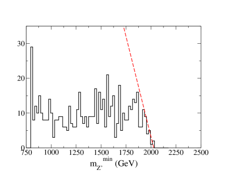
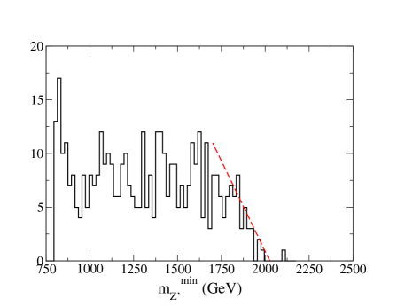
Figure 10: $m_{Z^{\prime}}^{min}$ constructed in each event with 130 $\rm fb^{-1}$ (L: $m_{\chi_{1}}=100$ GeV. Endpoint at $m_{Z^{\prime}}^{min}=2.028$ TeV. R: $m_{\chi_{1}}=250$ GeV. Endpoint at $m_{Z^{\prime}}^{min}=2.026$ TeV.)

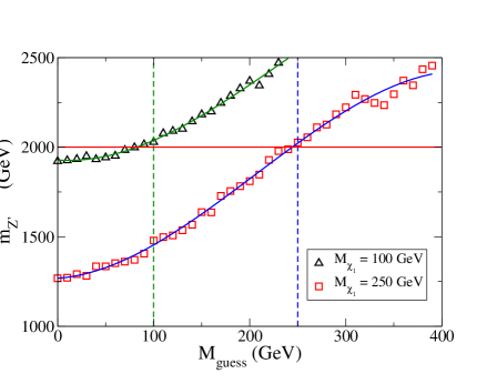
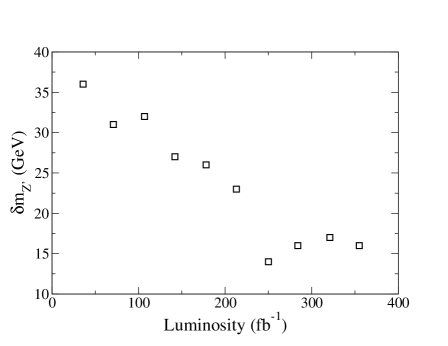
Figure 11: L: Endpoint of $m_{Z^{\prime}}^{min}$ constructed in each event vs. $M_{\rm{guess}}$ with integrated luminosity of 130 $\rm{fb}^{-1}$. R: Uncertainty in $m_{Z^{\prime}}^{min}$ endpoint vs. integrated luminosity ($m_{\chi_{1}}=100$ GeV)

$m_{\chi_{1}}=100$	$M_{\rm{guess}}=80$	$M_{\rm{guess}}=90$	$M_{\rm{guess}}=100$
$m_{Z^{\prime}}^{min}$ Endpoint	1998	2015	2028
$m_{\chi_{1}}=250$	$M_{\rm{guess}}=240$	$M_{\rm{guess}}=250$	$M_{\rm{guess}}=260$
$m_{Z^{\prime}}^{min}$ Endpoint	1988	2026	2055

Table 3: Endpoints of the distributions of minimum $m_{Z^{\prime}}^{min}$ calculated for each event (closest three to $m_{Z^{\prime}}+\Gamma_{Z^{\prime}}$). All quantities in GeV. Uncertainty is $\pm 27$ GeV.

4.3 $Z^{\prime}$ + Gravitino LSP

So far, we have only considered the simple decay $\tilde{\ell}\rightarrow\ell+\tilde{\chi}$. Models dominated by cascade decays are more complicated, but the kinematics of the additional final state particles allow for a richer analysis. As an example, we consider a model with a massless gravitino and a heavy $Z^{\prime}$, where the slepton decays through a short lived bino NLSP,

$$\tilde{\ell}\rightarrow\ell+\tilde{\chi}_{1}^{0}\rightarrow\ell+\gamma+\tilde{G}\,.$$

The events in figure 12 can be used to measure the masses of both the slepton and the NLSP. One approach is to treat the photons as “invisible” (by adding their transverse energy to $\not E_{T}$) and proceed with the $m_{T2}$ analysis described above. However, this requires an artificially large number of events because it ignores the valuable kinematic information of the photons. Another approach is to devise a suitable max-min variable for this decay chain using the strategy described in the previous section. In order to demonstrate a different method, we instead use a weighting scheme based on the photon momenta to determine $m_{\tilde{\ell}}$ and $m_{\chi_{1}}$ with a small number of events.

Figure 12: Decay of the $Z^{\prime}$ in a model with a massless gravitino and short-lived NLSP.

Our analysis is similar to the measurement of the top quark mass in the dilepton channel at D0, $t\bar{t}\rightarrow jj\nu\bar{\nu}\ell^{+}\ell^{-}$ [32]. In the case of the top quark, just 6 events were sufficient to measure the mass to an accuracy of 8%. In our case, there are two unknown masses instead of one, but there is also an additional constraint because each event starts with an on shell $Z^{\prime}$.

The spectrum, given in Table 4, is motivated by gauge mediated SUSY breaking, but with the additional twist that the messenger sector is charged under $U(1)_{B-L}$. This gives a contribution to the scalar masses proportional to $B-L$, lifting $m_{\tilde{\ell}}$ above the heaviest electroweak gaugino. One of the telltale signs of gauge mediation is a kinematic edge in the dilepton invariant mass distribution from the decay $\tilde{\chi}^{0}\rightarrow\tilde{\ell}+\ell\rightarrow\ell+\tilde{\chi}^{0}+\ell$, but this is forbidden in this model. On shell sleptons are produced only in the

decay of the $Z^{\prime}$.

Particle	Mass (GeV)
$Z^{\prime}$	2000
$\tilde{G}$	0
$\tilde{\chi}_{1}^{0}$ (mostly bino)	100
$\tilde{\ell}$	400

Table 4: SUSY spectrum with a gravitino LSP used in this analysis.

We studied an integrated luminosity of $100~{}\rm{fb}^{-1}$. Standard model background is negligible because of the two hard photons in the final state. Requiring two hard leptons, two hard photons, and no hard jets, we find 640 candidate events.

Given the mass of the $Z^{\prime}$ (which is easy to determine from another channel such as $Z^{\prime}\rightarrow e^{+}e^{-}$), the kinematics of the event in figure 12 are determined up to a single unknown. Therefore, for each such event, after imposing the constraints we are left with a one-parameter family of possible solutions for $m_{\tilde{\ell}}$ and $m_{\chi_{1}}$. Because the $Z^{\prime}$ has a finite width, and because the constraints are solved numerically on a coarse grid, the one parameter family of solutions is in practice a scattering of points in $m_{\tilde{\ell}}-m_{\chi_{1}}$ space.

All possible pairs $(m_{\tilde{\ell}}^{i},m_{\chi_{1}}^{i})$ that solve the constraints are not equally likely. Ideally, each pair should be weighted by the probability that it would produce the observed event,

$$W^{ideal}(\{p_{obs}\},m_{\tilde{\ell}}^{i},m_{\chi_{1}}^{i}) = P\left(\{p_{obs}\}\,|\,m_{\tilde{\ell}}=m_{\tilde{\ell}}^{i},m_{\chi_{1}}=m_{\chi_{1}}^{i}\right)dp_{obs}$$

where $\{p_{obs}\}$ are the observed four momenta of the leptons and photons. The full probability function is difficult to calculate, so instead we use a simplified weighting function based only on the photon transverse momenta $p_{t}^{1}$ and $p_{t}^{2}$,

$$W(\{p_{obs}\},m_{\tilde{\ell}}^{i},m_{\chi_{1}}^{i}) = P\left(p_{t}^{1},p_{t}^{2}\,|\,m_{\tilde{\ell}}=m_{\tilde{\ell}}^{i},m_{\chi_{1}}=m_{\chi_{1}}^{i}\right)dp_{t}^{1}dp_{t}^{2}\,.$$

Photon momentum was chosen because the distribution of lepton $p_{t}$ from this decay is relatively flat. PYTHIA was used to generate the photon $p_{t}$ distributions for 45 reference models with $300<m_{\tilde{\ell}}<600$ and $0<m_{\chi_{1}}<200$. Then, to compute the weighting function for each guess of $(m_{\tilde{\ell}}^{i},m_{\chi_{1}}^{i})$, the appropriate $p_{t}$ distribution was interpolated from the 45 reference models.

The total weight for each event is normalized to one. Finally, the weighted distributions for all 640 candidate events are added together, and the weighted frequency counts in each bin are interpreted as the “likelihood” of a given solution. The result is shown in figure 13. The maximal 5 GeV by 5 GeV bin is centered at $m_{\chi_{1}}=107.5$ GeV and $m_{\tilde{\ell}}=412.5$ GeV, which should be compared to the Monte Carlo input masses $m_{\chi_{1}}=100$ GeV and $m_{\tilde{\ell}_{R}}=400$ GeV. Clearly, this is a sensitive measurement of the slepton and NLSP masses; however, we have not done the Monte Carlo necessary to state reliable error bars. Even without a weighting function (i.e. $W=1$ for all observables), the maximum frequencies are found to be very close to the correct input masses.

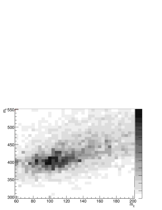
Figure 13: Weighted frequency of $m_{\chi_{1}},m_{\tilde{\ell}}$ masses found by reconstructing 640 candidate events in every way consistent with kinematic constrains. The input masses are $m_{\chi_{1}}=100$ GeV and $m_{\tilde{\ell}_{R}}=400$ GeV, and the maximal bin is centered at $m_{\chi_{1}}=107.5$ GeV, $m_{\tilde{\ell}}=412.5$ GeV.

5 Conclusions

Generically, we expect extensions of the gauge structure and the matter content of the MSSM. In this paper, we have studied the impact on supersymmetry phenomenology of $U(1)^{\prime}$ extensions of the minimal supersymmetric Standard Model. We have demonstrated that such an extension will give us a much stronger handle on the sleptons and electroweak-inos. Specifically, due to the enhanced slepton production cross section through $pp\rightarrow Z^{\prime}\rightarrow\tilde{\ell}\tilde{\ell}^{*}$, in comparison with the MSSM process $pp\rightarrow Z^{*}/\gamma^{*}\rightarrow\tilde{\ell}\tilde{\ell}^{*}$, we expect a greatly enhanced slepton discovery reach in this scenario. Moreover, with this additional source of on-shell sleptons, we have a much better handle on LSP identity. For example, simple signatures such as lepton counting reveal the existence of a chargino state degenerate with the LSP in the wino LSP scenario, distinguishing it from the bino-LSP case.

With an additional resonance, a $Z^{\prime}$ in our case, we have more kinematical information to measure the masses of the superpartners involved in the decay chain. We developed a new method to take advantage of such a constraint. Using this type of max-min variable in the analysis of our model allows us to completely determine the masses of the sleptons and the LSP. This class of observables should have a much wider range of applicability in more complicated decay chains. Like standard edges and endpoints, $m_{T2}$-like observables are particularly easy to implement because they do not require fitting parameters to a Monte Carlo simulation.

In a generic model where new particles are produced in pairs and the final state has only two invisible particles, max-min variables can be devised that give additional constraints beyond the usual constraints provided by edges and endpoints. In the simplest case, $pp\rightarrow\tilde{\ell}\tilde{\ell}\rightarrow\ell\ell\tilde{\chi}^{1}_{0}\tilde{\chi}^{1}_{0}$, there are no standard edges or endpoints but the original $m_{T2}$ variable gives one constraint. In a more complicated decay with more intermediate on shell particles, for instance the decay to gravitinos in Section 4.3, the edge in the $\ell\gamma$ invariant mass distribution gives one constraint on the two unknown masses and an appropriately designed max-min variable gives a second. As in the case of an on-shell $Z^{\prime}$, max-min variables can also be applied sequentially. The output of one variable can be used as the input to another applied higher in the decay chain.

In our study we have made the assumption that the sleptons are degenerate for simplicity. Since the purpose of our paper is demonstrating the effect of a new set of signals and observables, rather than a comprehensive study, this assumption should simply be viewed as a useful first step. We do not expect small and moderate mass splittings of order $100~{}\rm{GeV}$ to significantly affect the discovery reach since such a splitting should have little effect on the lepton $p_{T}$ and missing energy spectrum in figure 2. Making one of the sleptons heavier could in fact improve the discovery reach, as long as $Z^{\prime}\rightarrow\tilde{\ell}_{\rm L,R}$ are still both allowed, since the slepton will decay into harder leptons. If one of the sleptons becomes too heavy for the Z’ to decay into, we expect the signal significance to drop accordingly, depending on the change in the branching ratio to the remaining light slepton. For mass reconstruction, a method similar to the one we described, possibly by taking advantage of multiple end-points, should be applicable in the case of large L-R splitting.

There are several other obvious directions to extend our study. First of all, one should also consider the case where the $Z^{\prime}$ decays into electroweak-inos. For example, this would be the case if the PQ symmetry were gauged and mixed with this $U(1)^{\prime}$. Such channels will also allow us to have new windows into the structure of the electroweak-ino sector, which is generically difficult in the MSSM.

We have studied the decay channel of the $Z^{\prime}$ into sleptons, but its decay into squarks is also interesting to consider. In this case, we expect to be able to extract additional information about the quark sector, complementary to that of the QCD production of such states. For example, if the $Z^{\prime}$ couplings to the quark states are chiral, we could have an additional handle on the left-right splitting of the squarks.

Alternative extensions of the gauge structure of the MSSM will undoubtedly give rise to other novel features of phenomenology. It would be interesting to explore typical examples of such scenarios.

6 Acknowledgments

We would like to thank all members of the Harvard LHC olympics team: Nima Arkani-Hamed, Clifford Cheung, A. Liam Fitzpatrick, Aaron Pierce, Philip Schuster, Jesse Thaler, and Natalia Toro for stimulating discussions and collaborations in the early stage of this project. We also thank Christopher Lester and Tilman Plehn for useful discussions during the MCTP LHC Inverse Workshop, in particular concerning the $m_{T2}$ variable. The research of L.-T. W. is supported by DOE under contract DE-FG02-91ER40654. M.B., T.H and C.K. are supported by Harvard University.

References

- [1] For a summary, see, for example, G. Duckeck et al. [ATLAS Collaboration], CERN-LHCC-2005-022
- [2] B. C. Allanach et al., in Proc. of the APS/DPF/DPB Summer Study on the Future of Particle Physics (Snowmass 2001) ed. N. Graf, Eur. Phys. J. C 25, 113 (2002) [eConf C010630, P125 (2001)] [arXiv:hep-ph/0202233].
- [3] B. K. Gjelsten, D. J. Miller and P. Osland, JHEP 0506, 015 (2005) [arXiv:hep-ph/0501033].
- [4] D. J. Miller, P. Osland and A. R. Raklev, JHEP 0603, 034 (2006) [arXiv:hep-ph/0510356].
- [5] N. Arkani-Hamed, G. L. Kane, J. Thaler and L. T. Wang, JHEP 0608, 070 (2006) [arXiv:hep-ph/0512190].
- [6] F. del Aguila and L. Ametller, Phys. Lett. B 261, 326 (1991).
- [7] H. Baer, C. h. Chen, F. Paige and X. Tata, Phys. Rev. D 49, 3283 (1994) [arXiv:hep-ph/9311248].
- [8] J. L. Hewett and T. G. Rizzo, Phys. Rept. 183, 193 (1989).
- [9] A. E. Faraggi, D. V. Nanopoulos and K. j. Yuan, Nucl. Phys. B 335, 347 (1990).
- [10] A. E. Faraggi, string Phys. Lett. B 278, 131 (1992).
- [11] S. Chaudhuri, G. Hockney and J. D. Lykken, Nucl. Phys. B 469, 357 (1996) [arXiv:hep-th/9510241].
- [12] M. Cvetic and P. Langacker, Phys. Rev. D 54, 3570 (1996) [arXiv:hep-ph/9511378].
- [13] G. Cleaver, M. Cvetic, J. R. Espinosa, L. L. Everett and P. Langacker, Nucl. Phys. B 545, 47 (1999) [arXiv:hep-th/9805133].
- [14] G. Cleaver, M. Cvetic, J. R. Espinosa, L. L. Everett, P. Langacker and J. Wang, Phys. Rev. D 59, 055005 (1999) [arXiv:hep-ph/9807479].
- [15] J. Giedt, Annals Phys. 289, 251 (2001) [arXiv:hep-th/0009104].
- [16] A. E. Faraggi, Phys. Lett. B 499, 147 (2001) [arXiv:hep-ph/0011006].
- [17] M. Cvetic, G. Shiu and A. M. Uranga, Nucl. Phys. B 615, 3 (2001) [arXiv:hep-th/0107166].
- [18] M. Cvetic, P. Langacker and G. Shiu, Phys. Rev. D 66, 066004 (2002) [arXiv:hep-ph/0205252].
- [19] M. Baumgart et al., “The Harvard Blackbox,” 2nd LHC Olympics meeting at CERN, February 2006 [http://physics.harvard.edu/ hartman/harvardbox.pdf].
- [20] E. Boos et al. [CompHEP Collaboration], Nucl. Instrum. Meth. A 534, 250 (2004) [arXiv:hep-ph/0403113]. A. S. Belyaev et al., arXiv:hep-ph/0101232. A. Pukhov et al., arXiv:hep-ph/9908288.
- [21] T. Sjostrand, L. Lonnblad, S. Mrenna and P. Skands, arXiv:hep-ph/0308153.
- [22] Pretty Good Simulation of High Energy Collisions, John Conway http://www.physics.ucdavis.edu/ conway/research/software/pgs/pgs4-general.htm
- [23] G. Abbiendi et al. [OPAL Collaboration], Eur. Phys. J. C 33, 173 (2004) [arXiv:hep-ex/0309053].
- [24] [ALEPH Collaboration], arXiv:hep-ex/0511027.
- [25] M. Carena, A. Daleo, B. A. Dobrescu and T. M. P. Tait, Phys. Rev. D 70, 093009 (2004) [arXiv:hep-ph/0408098].
- [26] H. C. Cheng, B. A. Dobrescu and K. T. Matchev, Nucl. Phys. B 543, 47 (1999) [arXiv:hep-ph/9811316].
- [27] C. H. Chen, M. Drees and J. F. Gunion, arXiv:hep-ph/9902309.
- [28] C. G. Lester and D. J. Summers, Measuring masses of semi-invisibly decaying particles pair produced at hadron colliders, Phys. Lett. B 463, 99 (1999) [arXiv:hep-ph/9906349].
- [29] C. G. Lester, Model independent sparticle mass measurements at ATLAS. PhD thesis, Cambridge University, 2001. CAV-HEP 02/13
- [30] A. J. Barr, C. G. Lester, M. A. Parker, B. C. Allanach and P. Richardson, Discovering anomaly-mediated supersymmetry at the LHC, JHEP 0303, 045 (2003) [arXiv:hep-ph/0208214].
- [31] A. Barr, C. Lester and P. Stephens, m(T2): The truth behind the glamour, J. Phys. G 29, 2343 (2003) [arXiv:hep-ph/0304226].
- [32] B. Abbott et al. [D0 Collaboration], Phys. Rev. Lett. 80, 2063 (1998) [arXiv:hep-ex/9706014].