Probing the Noncommutative Standard Model at Hadron Colliders

Abstract

We study collider signals for the noncommutative extension of the standard model using the Seiberg-Witten maps for $\mathrm{SU}(3)_{C}\otimes\mathrm{SU}(2)_{L}\otimes\mathrm{U}(1)_{Y}$ to first order in the noncommutativity parameters $\theta_{\mu\nu}$. In particular, we investigate the sensitivity of $Z\gamma$-production at the Tevatron and the LHC to the components of $\theta_{\mu\nu}$. We discuss the range of validity of this approximation and estimate exclusion limits from a Monte Carlo simulation.

1 Introduction

The observation that the low energy limit of certain open string theories can be interpreted as Yang-Mills theories living on a noncommutative (NC) manifold [1] has raised renewed interest in noncommutative quantum field theories. Furthermore, Noncommutative Quantum Field Theory (NCQFT) in itself remains an appealing way to introduce a length scale and to cut off some short-distance contributions [2] consistently with the symmetries of a given model.

In the simplest case, the NC structure of spacetime is described by a set of constant c-number parameters $\theta^{\mu\nu}$, or, equivalently, by an energy scale $\Lambda_{\text{NC}}$ and dimensionless parameters $C^{\mu\nu}$:

$$[\hat{x}^{\mu},\hat{x}^{\nu}]=\mathrm{i}\theta^{\mu\nu}=\mathrm{i}\frac{1}{\Lambda_{\text{NC}}^{2}}C^{\mu\nu}=\mathrm{i}\frac{1}{\Lambda_{\text{NC}}^{2}}\begin{pmatrix}0&-E^{1}&-E^{2}&-E^{3}\\ E^{1}&0&-B^{3}&B^{2}\\ E^{2}&B^{3}&0&-B^{1}\\ E^{3}&-B^{2}&B^{1}&0\end{pmatrix}\,.$$ (1)

Here we have defined dimensionless “electric” and “magnetic” parameters $\vec{E}$ and $\vec{B}$ for convenience. Obviously, fixed non-vanishing values for $\theta^{\mu\nu}$ result in a breaking of Lorentz invariance. A possible mechanism of spontaneous breaking is the condensation of a rank two antisymmetric background field. In this paper, we will investigate phenomenological consequences of $\theta^{\mu\nu}$ at hadron colliders and not deal with the dynamics of the symmetry breaking mechanism.

Since the string scale is essentially unknown, we have also no prediction for $\Lambda_{\text{NC}}$. The current best collider tests [3] give $\Lambda_{\text{NC}}>140\,\mathrm{GeV}$ for a NC extension of QED, while experiments at a future photon collider are expected to reach 1 TeV [4]. Tests of rotation invariance in atomic physics and astrophysical tests give substantially higher bounds, but assume NC geometry at large scales (see [5] for a review).

Collider experiments do not probe space-time coordinates themselves, but functions of space-time coordinates, such as wave functions of external particles and effective Lagrangians. Consequently, one can employ a deformed product to describe the scattering theory on a given NC manifold by an equivalent scattering theory on a commuting manifold with new effective interactions. In the case of the operator algebra (1), one can use the Moyal-Weyl $\ast$-product [6]

$$(f\ast g)(x)=f(x)e^{\frac{\mathrm{i}}{2}\overleftarrow{\partial_{\mu}}\theta^{\mu\nu}\overrightarrow{\partial_{\nu}}}g(x)=f(x)g(x)+\frac{\mathrm{i}}{2}\theta^{\mu\nu}\frac{\partial f(x)}{\partial x^{\mu}}\frac{\partial g(x)}{\partial x^{\nu}}+\mathcal{O}(\theta^{2})$$ (2)

to map products of functions of NC coordinates, $(fg)(\hat{x})=f(\hat{x})g(\hat{x})$, to the equivalent products of functions on ordinary space-time coordinates, $(f\ast g)(x)$. It is easy to see that the commutation relation (1) is reproduced by the $\ast$-commutator:

$$[x^{\mu}\operatorname{\stackrel{{\scriptstyle\ast}}{{,}}}x^{\nu}](x)=(x^{\mu}\ast x^{\nu})(x)-(x^{\nu}\ast x^{\mu})(x)=\mathrm{i}\theta^{\mu\nu}=[\hat{x}^{\mu},\hat{x}^{\nu}]\,.$$ (3)

The obvious approach to constructing NCQFTs by replacing all field products by the $\ast$-product (2) fails for general gauge theories. For example, in such a NC version of QED all charged matter field must carry the same charge [7] which makes this approach unsuitable for the $\mathrm{U}(1)$ hypercharge of the standard model. Furthermore, this approach does not work for $\mathrm{SU}(N)$ gauge theories, because the $\ast$-commutator of two infinitesimal gauge transformations does not close in the $\mathrm{SU}(N)$ Lie algebra [8]:

$$[\alpha\operatorname{\stackrel{{\scriptstyle\ast}}{{,}}}\beta]=[\alpha^{a}T^{a}\operatorname{\stackrel{{\scriptstyle\ast}}{{,}}}\beta^{b}T^{b}]=\frac{1}{2}\{\alpha^{a}\operatorname{\stackrel{{\scriptstyle\ast}}{{,}}}\beta^{b}\}[T^{a},T^{b}]+\frac{1}{2}[\alpha^{a}\operatorname{\stackrel{{\scriptstyle\ast}}{{,}}}\beta^{b}]\{T^{a},T^{b}\}\,.$$ (4)

In order to circumvent these problems, we follow the approach of [8] and let the NC gauge field $\hat{A}$ and gauge parameter $\hat{\lambda}$ take their values in the enveloping algebra of the Lie algebra of the Standard Model (SM) gauge group $\mathrm{SU}(3)_{C}\otimes\mathrm{SU}(2)_{L}\otimes\mathrm{U}(1)_{Y}$. $\hat{A}$, $\hat{\lambda}$ and the NC matter fields $\hat{\psi}$ are expressed as nonlinear functions of ordinary fields $A$, $\lambda$ and $\psi$ via Seiberg-Witten maps (SWM) [1] such that the NC gauge transformations of the former,

$$\hat{\psi} \rightarrow\hat{\psi}^{\prime}=\mathrm{e}^{\mathrm{i}g\hat{\lambda}\ast}\hat{\psi}=\hat{\psi}+\mathrm{i}g\hat{\lambda}\ast\hat{\psi}+\frac{(\mathrm{i}g)^{2}}{2!}\hat{\lambda}\ast\hat{\lambda}\ast\hat{\psi}+\mathcal{O}(\hat{\lambda}^{3})$$ (5a)

$$\hat{A}_{\mu} \rightarrow\hat{A}_{\mu}^{\prime}=\mathrm{e}^{\mathrm{i}g\hat{\lambda}\ast}\hat{A}_{\mu}\mathrm{e}^{-\mathrm{i}g\hat{\lambda}\ast}+\frac{\mathrm{i}}{g}\mathrm{e}^{\mathrm{i}g\hat{\lambda}\ast}\left(\partial_{\mu}\mathrm{e}^{-\mathrm{i}g\hat{\lambda}\ast}\right)$$ (5b)

$$\phantom{\rightarrow\hat{A}_{\mu}^{\prime}}=\hat{A}_{\mu}+\mathrm{i}g[\hat{\lambda}\operatorname{\stackrel{{\scriptstyle\ast}}{{,}}}\hat{A}_{\mu}]+\frac{(\mathrm{i}g)^{2}}{2!}[\hat{\lambda}\operatorname{\stackrel{{\scriptstyle\ast}}{{,}}}[\hat{\lambda}\operatorname{\stackrel{{\scriptstyle\ast}}{{,}}}\hat{A}_{\mu}]]+\partial_{\mu}\hat{\lambda}+\mathrm{i}g[\hat{\lambda}\operatorname{\stackrel{{\scriptstyle\ast}}{{,}}}\partial_{\mu}\hat{\lambda}]+\mathcal{O}(\hat{\lambda}^{3})\,,$$

are realized by ordinary gauge transformations of the latter:

$$\psi \rightarrow\psi^{\prime}=\mathrm{e}^{\mathrm{i}g\lambda}\psi=\psi+\mathrm{i}g\lambda\psi+\frac{(\mathrm{i}g)^{2}}{2!}\lambda^{2}\psi+\mathcal{O}(\lambda^{3})$$ (6a)

$$A_{\mu} \rightarrow A_{\mu}^{\prime}=\mathrm{e}^{\mathrm{i}g\lambda}A_{\mu}\mathrm{e}^{-\mathrm{i}g\lambda}+\frac{\mathrm{i}}{g}\mathrm{e}^{\mathrm{i}g\lambda}\left(\partial_{\mu}\mathrm{e}^{-\mathrm{i}g\lambda}\right)$$ (6b)

$$\phantom{\rightarrow A_{\mu}^{\prime}}=A_{\mu}+\mathrm{i}g[\lambda,A_{\mu}]+\frac{(\mathrm{i}g)^{2}}{2!}[\lambda,[\lambda,A_{\mu}]]+\partial_{\mu}\lambda+\mathrm{i}g[\lambda,\partial_{\mu}\lambda]+\mathcal{O}(\lambda^{3})\,.$$

This leads to the so-called gauge-equivalence conditions

$$\hat{A}(A,\theta) \to\hat{A}^{\prime}(A,\theta)=\hat{A}(A^{\prime},\theta)$$ (7a)

$$\hat{\lambda}(\lambda,A,\theta) \to\hat{\lambda}^{\prime}(\lambda,A,\theta)=\hat{\lambda}(\lambda^{\prime},A^{\prime},\theta)$$ (7b)

$$\hat{\psi}(\psi,A,\theta) \to\hat{\psi}^{\prime}(\psi,A,\theta)=\hat{\psi}(\psi^{\prime},A^{\prime},\theta)\,,$$ (7c)

that can be solved order by order in $\theta^{\mu\nu}$. The first order is given by

$$\hat{A}_{\mu}(x) =A_{\mu}(x)+\frac{1}{4}\theta^{\rho\sigma}\left\{A_{\sigma}(x),\partial_{\rho}A_{\mu}(x)+F_{\rho\mu}(x)\right\}+\mathcal{O}(\theta^{2})$$ (8a)

$$\hat{\psi}(x) =\psi(x)+\frac{1}{2}\theta^{\rho\sigma}A_{\sigma}(x)\partial_{\rho}\psi(x)+\frac{\mathrm{i}}{8}\theta^{\rho\sigma}\left[A_{\rho}(x),A_{\sigma}(x)\right]\psi(x)+\mathcal{O}(\theta^{2})$$ (8b)

$$\hat{\lambda}(x) =\lambda(x)+\frac{1}{4}\theta^{\rho\sigma}\left\{A_{\sigma}(x),\partial_{\rho}\lambda(x)\right\}+\mathcal{O}(\theta^{2})$$ (8c)

with $F_{\mu\nu}=(\mathrm{i}/g)[D_{\mu},D_{\nu}]$. The SWM approach also solves the charge quantization problem by introducing a separate NC gauge field for each eigenvalue of the $\mathrm{U}(1)$ charge operator. Each of these gauge fields is subsequently mapped by the SWM to the same SM $\mathrm{U}(1)$ field. Thus no additional degrees of freedom appear. This approach has been used to construct a NC generalization of the complete electroweak standard model [9], which will be referred to as NCSM below.

This construction leads to modifications of the familiar SM interaction vertices as well as to new interactions that are forbidden in the SM. The most striking feature of the NCSM is that it allows direct interactions among neutral gauge bosons, depending on the representation of the enveloping algebra chosen for the trace in the gauge boson Lagrangian [9]

$$\mathcal{L}=-\frac{1}{2}\operatorname{tr}\Bigl{(}F_{\mu\nu}F^{\mu\nu}\Bigr{)}\,.$$ (9)

Note that all representations are equivalent up to a renormalization only in the case of Lie algebras, but not in the corresponding enveloping associative algebra.

We should point out that NC gauge theories constructed from commutative gauge theories using the SWM are not renormalizable by field and gauge coupling renormalization alone, since the $4$-point functions of matter fields require additional counterterms that can not be obtained from the application of the SWM [10]. Nevertheless, the NCSM can be employed as a well defined effective field theory, because any chiral model that is constructed from an anomaly free chiral model using the SWM has been shown to be anomaly free [11].

To first order in $\theta^{\mu\nu}$, all modifications of the SM correspond to effective dimension-six operators. The latter lead to observable deviations from the SM predictions or, in the absence of deviations, to bounds on $\Lambda_{\text{NC}}$. Initially, most phenomenological studies have focused on rare and $B$-decays [12], while tests at future colliders have been considered in [4]. Additional phenomenological results have been presented in [13].

In this paper, we report on a phenomenological study of the NCSM in first order in $\theta^{\mu\nu}$, concentrating on the process $pp/p\bar{p}\to\ell^{+}\ell^{-}\gamma$ at hadron colliders. We shall point out experimental signatures unique to the NCSM and estimate the range of the NC scale $\Lambda_{\text{NC}}$ that can be probed at the Tevatron and the LHC. The paper is structured as follows: In section 2, we discuss the scattering amplitude that gives rise to the signals described in section 3. In section 4, we analyse the results of our Monte Carlo (MC) simulations and estimate the discovery reach. Section 5 gives a short outlook on future work. Feynman rules and analytical results for the cross section are presented in the appendix.

2 Partonic Scattering Amplitudes and Cross Sections

The pair production of neutral electroweak gauge bosons $V=\gamma,Z$ at a hadron collider is described by the partonic process $q\bar{q}\to VV^{\prime}$. The corresponding squared matrix element at $\mathcal{O}(\theta)$ is given by

$$|A|^{2}=|A^{\text{SM}}+A^{\text{NC}}|^{2}=|A^{\text{SM}}|^{2}+2\mathrm{Re}\left(A^{*\,\text{SM}}A^{\text{NC}}\right)+O(\theta^{2})$$ (10)

where $A^{\text{SM}}=A^{\text{SM}}_{t}+A^{\text{SM}}_{u}$ is the SM amplitude with

$$A^{\text{SM}}_{t}=\parbox{102.42992pt}{\includegraphics{nclhc-pics-1}}\qquad A^{\text{SM}}_{u}=\parbox{102.42992pt}{\includegraphics{nclhc-pics-2}}$$ (11)

and

$$A^{\text{NC}}=\sum_{i=1,2}(A^{\text{NC}}_{t,i}+A^{\text{NC}}_{u,i})+A^{\text{NC}}_{c}+A^{\text{NC}}_{s,\gamma}+A^{\text{NC}}_{s,Z}\,,$$ (12)

denotes the new contributions arising in the NCSM. The relevant Feynman rules are provided in appendix A. Below, the $\mathcal{O}(\theta)$ contributions to the SM vertices (24q) have been marked by an open box in the corresponding SM Feynman diagrams:

$$A^{\text{NC}}_{t,1} =\parbox{102.42992pt}{\includegraphics{nclhc-pics-3}} A^{\text{NC}}_{t,2} =\parbox{102.42992pt}{\includegraphics{nclhc-pics-4}}$$ (13a)

$$A^{\text{NC}}_{u,1} =\parbox{102.42992pt}{\includegraphics{nclhc-pics-5}} A^{\text{NC}}_{u,2} =\parbox{102.42992pt}{\includegraphics{nclhc-pics-6}}\,.$$ (13b)

The contact term

$$A^{\text{NC}}_{c}=\parbox{102.42992pt}{\includegraphics{nclhc-pics-7}}\,,$$ (13c)

with the vertex given in (24r), is required by gauge invariance, as can be seen from the Ward identity (14a). In contrast, the two $$s$$-channel diagrams

$$A^{\text{NC}}_{s,\gamma}=\parbox{102.42992pt}{\includegraphics{nclhc-pics-8}}\qquad A^{\text{NC}}_{s,Z}=\parbox{102.42992pt}{\includegraphics{nclhc-pics-9}}$$ (13d)

involving the triple gauge boson couplings given in (24s) are separately gauge invariant. The corresponding Ward identities

$$k_{1,\mu}\Bigl{(}\sum_{i=1}^{2}(A^{\text{NC}}_{t,i}+A^{\text{NC}}_{u,i})+A^{\text{NC}}_{c}\Bigr{)}^{\mu\nu}\varepsilon_{\nu}(k_{2}) =0$$ (14a)

$$k_{1\mu}(A^{\text{NC}}_{s,\gamma})^{\mu\nu}\varepsilon_{\nu}(k_{2})=k_{1\mu}(A^{\text{NC}}_{s,Z})^{\mu\nu}\varepsilon_{\nu}(k_{2}) =0\,.$$ (14b)

have been proven in [4]. The separate gauge invariance of $A^{\text{NC}}_{s,\gamma}$ and $A^{\text{NC}}_{s,Z}$ is not surprising, because the strength of the triple gauge boson interactions depends on the choice of representation of the enveloping algebra [9] used for the gauge field Lagrangian (9). The new coupling constants $K_{Z\gamma\gamma}$ and $K_{ZZ\gamma}$ are only constrained by the matching to the SM in the limit $\theta^{\mu\nu}\to 0$ and can vary independently in a finite range [9], as illustrated in fig. 1.

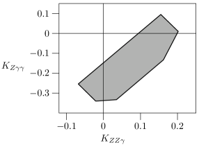
Figure 1: Range for the triple neutral gauge boson couplings $K_{Z\gamma\gamma}$ and $K_{ZZ\gamma}$ allowed by the matching to the SM in the limit $\theta^{\mu\nu}\to 0$ in the nonminimal NCSM, as defined in [9].

It has been shown [4] for $\gamma\gamma$-collisions that polarization is essential for obtaining a non-vanishing signal in $\mathcal{O}(\theta)$. At the LHC one will not have polarized initial states, neither can one expect to observe the polarization of outgoing photons or use $Z$-decays as a polarimeter. Therefore, we have concentrated on unpolarized $Z\gamma$-production. The analytical result for $\mathrm{d}\sigma(q\bar{q}\to Z\gamma)/\mathrm{d}\Omega$ is presented in appendix B.

Without polarization, the most important observable, i. e. an azimuthal dependence of the cross section, vanishes for symmetric initial and final states, as we will see in section 3. In the present case, it is the axial coupling of the $Z$ that will engender an observable deviation from the SM prediction. Since the width of the intermediate $Z$ is negligible for $\sqrt{\hat{s}}\gg m_{Z}$, one needs another source for an imaginary part in the scattering amplitudes to compensate the factor of $\mathrm{i}$ that comes with $\theta^{\mu\nu}$ and to obtain a non-vanishing contribution to the $\mathcal{O}(\theta)$ interference. In polarized scattering, the polarization vectors and spinors can provide this imaginary part, but all the polarization sums are real, of course. However, the $\gamma^{5}$ factor in the axial coupling of the $Z$ produces a factor $\mathrm{i}\epsilon^{\mu\nu\rho\sigma}$ after tracing and thus creates a non-vanishing effect from contractions with the three independent momenta and $\theta^{\mu\nu}$.

3 Distributions and Signals in $pp/p\bar{p}\to Z\gamma$

The relevant hadronic processes are $pp\to Z\gamma$ at the LHC and $p\bar{p}\to Z\gamma$ at the Tevatron with subsequent decays of the $Z$ into $e^{+}e^{-}$ and $\mu^{+}\mu^{-}$. For these, the cross sections and lepton distributions have been calculated using the results for the hard $q\bar{q}\to\ell^{+}\ell^{-}\gamma$ cross sections from section 2 together with the phase space generation and parton distribution functions provided by WHiZard [14] for Monte Carlo simulation.

As expected for new short distance physics, we observe a deviation of the photon $p_{T}$ distribution at high $p_{T}$ from the SM prediction. However, this deviation is not specific to the NCSM and, in addition, turns out to be smaller than a few $\%$ for $p_{T}\lesssim\Lambda_{\text{NC}}/2$. On the other hand, the NC parameter $\theta^{\mu\nu}$ breaks rotational invariance and leads to a characteristic dependence of the cross sections on the azimuthal angle $\phi$, which can be used to discriminate against other new physics effects. For this reason, we have focussed our phenomenological analysis on the azimuthal distribution of the photon.

As has been shown previously [4], the $\gamma\gamma\to f\bar{f}$ amplitude in the NCSM depends only on $E_{1}$ and $E_{2}$. In contrast, the $f\bar{f}\to Z\gamma$ amplitude also depends on $B_{1}$ and $B_{2}$, due to the axial $Zf\bar{f}$ couplings. In addition, a dependence on $E_{3}$ appears because the vector bosons are not aligned with the beam axis $x_{3}$. Nevertheless, the CMS parton cross sections show a much stronger dependence on the components $\vec{E}$ than on $\vec{B}$, as exemplified in fig. 2. To be precise, this is true everywhere except sufficiently close to the polar angle $\theta^{*}=\pi/2$, where the dependence on $\vec{E}$ vanishes due to the antisymmetry of the $\mathcal{O}(\theta)$ contribution to $\mathrm{d}\sigma/\mathrm{d}\Omega^{*}$ in $\cos\theta^{*}$.

Figure 2: Azimuthal distribution of the $\gamma$ in $q\bar{q}\to Z\gamma$ at fixed CMS energy $\sqrt{\hat{s}}$ for $\vec{E}=(1,0,0)$ and $\cos\theta^{*}=0.05\text{(full)},-0.05\text{(dashed)}$, in comparison with $\vec{B}=(0,1,0)$ for $\cos\theta^{*}=\pm 0.05\text{(dotted)}$.

However, at hadron colliders, the partonic CMS of most events is boosted significantly along the beam axis. As is well known from electrodynamics, $\vec{E}$ and $\vec{B}$ are mixed by Lorentz boosts along the beam axis $x_{3}$:

$$E_{1} \to\gamma(E_{1}-\beta B_{2}) \quad B_{1} \to\gamma(B_{1}+\beta E_{2})$$ (15)

$$E_{2} \to\gamma(E_{2}+\beta B_{1}) \quad B_{2} \to\gamma(B_{2}-\beta E_{1})$$

$$E_{3} \to E_{3} \quad B_{3} \to B_{3}$$

($\gamma=1/\sqrt{1-\beta^{2}}$, $\beta=v/c$). The measurements of $(E_{1},B_{2})$ and $(E_{2},B_{1})$, respectively, are therefore highly correlated by kinematics. We have verified that the strenght of the correlation is essentially determined by the expectation value of the boost $\langle|\beta|\rangle$.

Calculating the scattering amplitude only to first order in the noncommutativity $\theta^{\mu\nu}$, one must neglect the $\mathcal{O}(\theta^{2})$ contributions in the squared amplitude for consistency. Therefore, in this approximation, the deviations from the SM only come from the interference of $A^{\text{SM}}$ with $A^{\text{NC}}$ in (10). As a consequence, the $\mathcal{O}(\theta)$ cross section can even become negative in some regions of phase space for sufficiently large absolute values and appropriate signs of components of $\theta^{\mu\nu}$, such that the NC/SM interference dominates over the SM contribution. The relative size of the interference term is determined by $\hat{s}/\Lambda_{\text{NC}}^{2}$, $\sqrt{\hat{s}}$ being the partonic CMS energy. There is a wide range of possible values of $\sqrt{\hat{s}}$ in high energy hadron collisions, but the most statistics will be collected at moderate values of $\sqrt{\hat{s}}$. Thus in $\mathcal{O}(\theta)$, values of $\Lambda_{\text{NC}}$ that cause observable deviations at such moderate values of $\sqrt{\hat{s}}$ can lead to unphysical cross sections at the highest $\sqrt{\hat{s}}$ available. This problem is not specific to simulations in the NCSM, but common to all studies of new physics that can be parametrized by anomalous couplings. A pragmatic solution is to unitarize the contributions from new physics by applying appropriate form factors that cut off the unphysical effects. Since there are very few events to be expected at the highest CMS energies, the conclusions should not depend on the details of the form factors. Therefore, we have simply replaced $\mathrm{d}\sigma/\mathrm{d}\Omega^{*}$ by $\max(\mathrm{d}\sigma/\mathrm{d}\Omega^{*},0)$ everywhere in our simulations.

This solution is also legitimized by the expectation that higher orders in $\theta^{\mu\nu}$ will damp the large negative interference contributions. In fact, preliminary results to second order in $\theta^{\mu\nu}$ support this expectation [15].

4 Sensitivity Estimates

In order to obtain a realistic estimate of the sensitivity at the Tevatron and the LHC, one has to take into account backgrounds, detector effects and selection cuts. Clearly, a comprehensive analysis of all reducible backgrounds and detector effects is beyond the scope of a theoretical study and must eventually be performed by the experimental collaborations. However, the final states under consideration are simple enough for a phenomenological analysis based on simple cuts. Moreover, experience at the Tevatron [16, 17] indicates that the combined detection efficiency for $\ell^{+}\ell^{-}\gamma$ can be assumed to be larger than $50\%$. All numerical results presented below are obtained for a $100\%$ efficiency. Smaller uniform efficiencies can easily be taken into account by scaling up the integrated luminosity accordingly.

We have simulated the process $pp\to\ell^{+}\ell^{-}\gamma$ at $\sqrt{s}=14\,\mathrm{TeV}$ using the program package WHiZard [14] and demanding the following acceptance cuts on leptons and photons:

$$E(\ell^{\pm}),E(\gamma) \geq 10\,\mathrm{GeV}$$ (16a)

$$\theta(\ell^{\pm}),\theta(\gamma) \geq 5^{\circ}$$ (16b)

$$\theta(\ell^{\pm}),\theta(\gamma) \leq 175^{\circ}$$ (16c)

$$p_{T}(\ell^{\pm}),p_{T}(\gamma) \geq 10\,\mathrm{GeV}\,.$$ (16d)

For the Tevatron, we have simulated $p\bar{p}\to\ell^{+}\ell^{-}\gamma$ at $\sqrt{s}=1.96\,\mathrm{TeV}$ using the same acceptance cuts (16).

For simplicity, we have assumed that the components of $\theta^{\mu\nu}$ remain aligned with the beam axis and the detector over the time of the measurement. This assumption is not justified, because we should expect that $\theta^{\mu\nu}$ is aligned with a fixed cosmic reference frame, that is determined by the dynamics of the underlying string theory. Therefore the alignment of the detector must be recorded with each event and the combined effect of the earth’s rotation and revolution must be taken into account. This poses no principal difficulty and will not change our conclusions.

4.1 Background Suppression

The hard scattering process $q\bar{q}\to Z\gamma$ (13) with subsequent decays $Z\to\ell^{+}\ell^{-}$ has the Drell-Yan process $q\bar{q}\to\ell^{+}\ell^{-}$ with photon radiation and $q\bar{q}\to\gamma^{*}\gamma$ with $\gamma^{*}\to\ell^{+}\ell^{-}$ as irreducible backgrounds. Both have been taken into account in our calculation.

As explained in section 2, the unpolarized azimuthal distribution in $q\bar{q}\to\gamma^{*}\gamma$ is flat. We suppress this background by requiring

$$|M(\ell^{+}\ell^{-})-M_{Z}|\leq\Gamma_{Z}\,.$$ (17)

In order to also reduce the radiative Drell-Yan events, we have applied an angular separation cut of

$$\Delta R_{\ell^{\pm}\gamma}=\sqrt{\Delta\eta^{2}+\Delta\phi^{2}}>0.7$$ (18)

(cf. [16, 17]). Finally, we require a minimum and maximum total energy in the partonic CMS:

$$200\,\mathrm{GeV}\leq|M(\ell^{+}\ell^{-}\gamma)|\leq 1\,\mathrm{TeV}\,.$$ (19)

The lower cut enriches the signal, while the upper cut reduces the influence of the elimination of the unphysical parton cross sections discussed in section 3.

At the LHC, $q\bar{q}$- and $\bar{q}q$-collisions will occur with identical rates. As shown in fig. 2, the dominant $E_{1}$ and $E_{2}$ contributions to the deviation of the parton cross sections from the SM prediction is antisymmetric in $\cos{\theta^{*}}$ and will therefore cancel for $pp$ initial states unless additional cuts are applied that separate events originating from $q\bar{q}$ and $\bar{q}q$.

In the proton, the average momentum fraction of the light valence quarks is much higher than that of the anti-quarks which exist only in the sea. As a result, all $q\bar{q}$-events will be boosted strongly in the direction of the quark. Therefore we can enrich our samples of signal events by requiring a minimal boost in the appropriate direction. We have found that demanding the momenta of both the photon and the lepton pair to lie in the same hemisphere in the laboratory frame, that is

$$\cos{\theta_{\gamma}}\cdot\cos{\theta_{\ell^{+}\ell^{-}}}>0$$ (20)

produces a nice signal, as displayed in fig. 3. In the figure, we have chosen a rather low value of $\Lambda_{\text{NC}}=0.6\,\text{TeV}$ for illustration. The values of $K_{Z\gamma\gamma}$ and $K_{ZZ\gamma}$ correspond to the top corner of the polygon in fig. 1.

In the case of the Tevatron, the rôle of quarks and anti-quarks are reversed in the antiproton. Therefore, we demand in this case that the momenta of the photon and the lepton pair lie in opposite hemispheres. For sufficiently small $\Lambda_{\text{NC}}$, the azimuthal distribution of the $\gamma$ is similar to the distribution plotted in fig. 3.

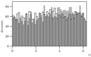
Figure 3: Azimuthal distributions of the $\gamma$ in $pp\to e^{+}e^{-}\gamma$ at the LHC, $\sqrt{s}=14\,\text{TeV}$, $300\,\text{fb}^{-1}$, for $\cos\theta_{e^{+}e^{-}}>0$, $\cos\theta_{\gamma}>0$, $0<\cos\theta^{*}_{\gamma}<0.9$ in the SM (open) and the NCSM (full) with $\Lambda_{\text{NC}}=0.6\,\text{TeV}$, $\vec{E}=(1,0,0)$, $K_{Z\gamma\gamma}=0.095$, $K_{ZZ\gamma}=0.155$.

4.2 Likelihood Fits

In the following, we analyze the NC effects on the azimuthal dependence of the unpolarized cross section stemming from the components $E_{1},E_{2},B_{1},B_{2}$ of $\theta_{\mu\nu}$. We disregard the small contribution from $E_{3}$, since, by symmetry, it has no influence on the azimuthal distribution.

Furthermore, we have taken advantage of the fact that the deviation of the cross section from the SM prediction is linear in $\theta_{\mu\nu}$ so that the corresponding binned $\chi^{2}$-function

$$\chi^{2}(E_{1},E_{2},B_{1},B_{2})=\sum_{i}\frac{1}{n^{\text{SM}}_{i}}\left(n^{\text{NC}}_{i}-n^{\text{SM}}_{i}\right)^{2}$$ (21)

depends quadratically on $\theta_{\mu\nu}$:

$$\chi^{2}(E_{1},E_{2},B_{1},B_{2})=\frac{1}{2}(E_{1},E_{2},B_{1},B_{2})X^{2}(E_{1},E_{2},B_{1},B_{2})^{T}\,,$$ (22)

up to statistical fluctuations. The elements of the matrix $X^{2}$ in (22) are then determined from a fit of $\chi^{2}(E_{1},E_{2},B_{1},B_{2})$ to the right-hand side of (21) for a sufficiently large grid of values $(E_{1},E_{2},B_{1},B_{2})$. Subsequently, we can diagonalize $X^{2}$ and obtain the error ellipses that describe the experimental reach of collider experiments.

4.3 Results

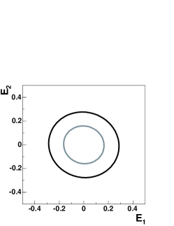
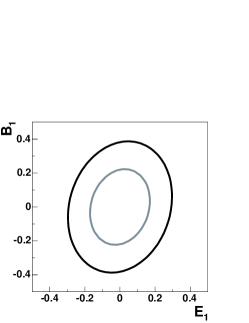
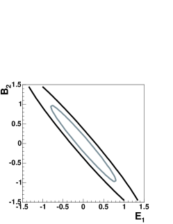
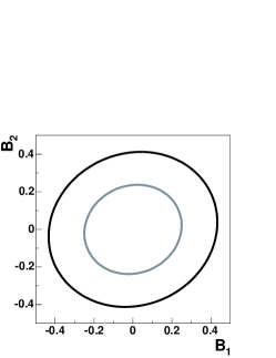
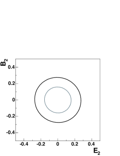
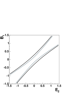
Figure 4: The $1\sigma$ (dark) and $3\sigma$ (light) exclusion contours for $\Lambda_{\text{NC}}=500\,\mathrm{GeV}$ and $100\,\mathrm{fb^{-1}}$ at the LHC discussed in the text.

For the LHC, the results of the likelihood fits are shown in fig. 4, setting $\Lambda_{\text{NC}}=500\,\mathrm{GeV}$ and $K_{Z\gamma\gamma}=K_{ZZ\gamma}=0$. From the error ellipses in the first and second column of fig. 4, we derive the following sensitivity limit on the NC scale for an integrated luminosity of $100\,\textrm{fb}^{-1}$ (with $100\%$ detection efficiency):

$$\Lambda_{\mathrm{NC}}\geq 1\,\mathrm{TeV}\;\text{for}\;|\vec{E}|^{2}+|\vec{B}|^{2}=1\,.$$ (23)

In the presence of triple gauge couplings among neutral gauge bosons, these limits do not change significantly. This analysis indicates that the current collider bounds [3] can be improved at the LHC by an order of magnitude.

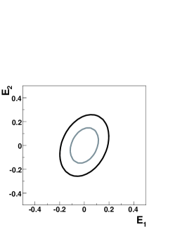
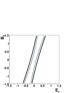
Figure 5: The $1\sigma$ (dark) and $3\sigma$ (light) exclusion contours for $\Lambda_{\text{NC}}=50\,\mathrm{GeV}$ and $15\,\mathrm{fb^{-1}}$ at the Tevatron discussed in the text.

A similar analysis of the likelihood fits for the Tevatron, shown in fig. 5, for $\int\mathcal{L}=15\,\mathrm{fb^{-1}}$ implies that the sensitivity on the NC scale reaches $\Lambda_{\textrm{NC}}\sim 130\,\mathrm{GeV}$, which is comparable to existing LEP bounds [3].

As expected from the Lorentz boost $(\ref{eq:correlation})$, we find that in the laboratory frame measurements of $E_{1}$ are correlated with $B_{2}$ and measurements of $E_{2}$ with $B_{1}$. The corresponding $1\sigma$ and $3\sigma$ contours are depicted for $\Lambda_{\text{NC}}=500\,\mathrm{GeV}$ in the right column of fig. 4. Since the dependence on $B_{1}$ and $B_{2}$ in the partonic CMS is very weak, one expects very elongated ellipses in the laboratory frame, in agreement with our result. Due to statistical fluctuations, the fitted matrix $X^{2}$ can have a negative eigenvalue, as happened in the bottom right plot of fig. 4. This sign is unphysical and as expected changes with the random number sequence used in the simulations. For all practical purposes, the error ellipses for $(E_{1},B_{2})$ and $(E_{2},B_{1})$ should be viewed as straight lines.

In the other pairs $(E_{1},E_{2})$, $(B_{1},B_{2})$ and $(E_{i},B_{i})$, we find no correlations. Indeed, the only source of violation of rotational invariance is $\theta^{\mu\nu}$ itself. Therefore no correlations between $E_{1}$ and $E_{2}$, as well as between $B_{1}$ and $B_{2}$, are expected since the measurements are related by a rotation around the beam axis by $\pi/2$.

Having established the absence of correlations that are not of purely kinematical origin, one can avoid expensive non-linear $4$-parameter fits in subsequent work that will take higher orders in $\theta^{\mu\nu}$ into account [15].

5 Conclusions and Outlook

We have studied the effect of a noncommutative extension of the SM on the production of neutral vector bosons at the LHC and the Tevatron. We have shown that, under conservative assumptions, values for the NC scale of $\Lambda_{\text{NC}}\gtrsim 1\,\mathrm{TeV}$ can be probed at the LHC, while the Tevatron is able to confirm existing limits.

The analysis has been performed to first order in $\theta^{\mu\nu}$. In this approximation, unphysical cross sections appear for large $\sqrt{\hat{s}}$ and for $\Lambda_{\text{NC}}$ in the region of sensitivity. These have been handled by a pragmatic regularization described in section 3 and appropriate kinematical cuts. On general grounds, one expects the problem to disappear when higher orders in $\theta^{\mu\nu}$ are taken into account. Preliminary results for the second order contributions confirm this expectation. We also find that cancellations in the unpolarized cross sections at $\mathcal{O}(\theta)$ are not effective in higher orders, allowing also studies of processes with symmetric final states like $pp\to\gamma\gamma$, one of the most important channels at the LHC. Therefore, the derivation of Seiberg-Witten maps for $\mathrm{SU}(3)_{C}\otimes\mathrm{SU}(2)_{L}\otimes\mathrm{U}(1)_{Y}$ of the corresponding NCSM in higher orders is important for a comprehensive analysis of the NCSM at the LHC.

The construction of the NCSM in $\mathcal{O}(\theta^{2})$ and further phenomenological tests, including $\gamma\gamma$ final states, will be presented in future publications [15].

Acknowledgments

This research is supported by Deutsche Forschungsgemeinschaft, grant RU 311/1-1, Research Training Group 1147 Theoretical Astrophysics and Particle Physics and by Bundesministerium für Bildung und Forschung Germany, grant 05HT4WWA/2. A. A. gratefully acknowledges support from Evangelisches Studienwerk e. V. Villigst.

Appendix A Feynman Rules

The Feynman rules corresponding to the NCSM Lagrangian [9] have been derived in [4, 18]. Here, we collect only the neutral current couplings entering our analysis. Choosing all momenta as incoming and using the shorthand notation $p\theta q=p_{\mu}q_{\nu}\theta^{\mu\nu}$ and $p\theta^{\nu}=p_{\mu}\theta^{\mu\nu}$, one has

$$=\frac{1}{2}(g_{V}+g_{A}\gamma_{5})\left(k\theta p\gamma^{\alpha}+p\theta^{\alpha}\mathchoice{\ooalign{$\hfil\displaystyle\mkern 0.0mu/\hfil$\crcr$\displaystyle k$}}{\ooalign{$\hfil\textstyle\mkern 0.0mu/\hfil$\crcr$\textstyle k$}}{\ooalign{$\hfil\scriptstyle\mkern 0.0mu/\hfil$\crcr$\scriptstyle k$}}{\ooalign{$\hfil\scriptscriptstyle\mkern 0.0mu/\hfil$\crcr$\scriptscriptstyle k$}}-k\theta^{\alpha}\mathchoice{\ooalign{$\hfil\displaystyle\mkern 0.0mu/\hfil$\crcr$\displaystyle p$}}{\ooalign{$\hfil\textstyle\mkern 0.0mu/\hfil$\crcr$\textstyle p$}}{\ooalign{$\hfil\scriptstyle\mkern 0.0mu/\hfil$\crcr$\scriptstyle p$}}{\ooalign{$\hfil\scriptscriptstyle\mkern 0.0mu/\hfil$\crcr$\scriptscriptstyle p$}}\right)$$ (24q)

$$\begin{aligned} =\frac{1}{2}&(g_{V}+g_{A}\gamma_{5})(g^{\prime}_{V}+g^{\prime}_{A}\gamma_{5})\cdot\\ &\biggl{(}\theta^{\alpha\beta}(\mathchoice{\ooalign{$\hfil\displaystyle\mkern 0.0mu/\hfil$\crcr$\displaystyle q$}}{\ooalign{$\hfil\textstyle\mkern 0.0mu/\hfil$\crcr$\textstyle q$}}{\ooalign{$\hfil\scriptstyle\mkern 0.0mu/\hfil$\crcr$\scriptstyle q$}}{\ooalign{$\hfil\scriptscriptstyle\mkern 0.0mu/\hfil$\crcr$\scriptscriptstyle q$}}-\mathchoice{\ooalign{$\hfil\displaystyle\mkern 0.0mu/\hfil$\crcr$\displaystyle k$}}{\ooalign{$\hfil\textstyle\mkern 0.0mu/\hfil$\crcr$\textstyle k$}}{\ooalign{$\hfil\scriptstyle\mkern 0.0mu/\hfil$\crcr$\scriptstyle k$}}{\ooalign{$\hfil\scriptscriptstyle\mkern 0.0mu/\hfil$\crcr$\scriptscriptstyle k$}})+(k-q)\theta^{\beta}\gamma^{\alpha}+(q-k)\theta^{\alpha}\gamma^{\beta}\biggr{)}\end{aligned}$$ (24r)

$$=\left\{\begin{aligned} &\;+2e\sin(2\theta_{W})\,K_{Z\gamma\gamma}\cdot V_{\mu_{1}\mu_{2}\mu_{3}}(k_{1},k_{2},k_{3})\\ &\;-2e\sin(2\theta_{W})\,K_{\gamma\gamma\gamma}\cdot V_{\mu_{1}\mu_{2}\mu_{3}}(k_{1},k_{2},k_{3})\end{aligned}\right.\,.$$ (24s)

In the above, the SM vector and axial-vector couplings in the fermion vertices are given by

$$g_{V} =T_{3}-2Q\sin^{2}\theta_{W}$$ (25a)

$$g_{A} =T_{3}\,$$ (25b)

while in the $$\gamma_{\mu_{1}}(k_{1})\gamma_{\mu_{2}}(k_{2})Z_{\mu_{3}}(k_{3}) \gamma_{\mu_{1}}(k_{1})Z_{\mu_{2}}(k_{2})Z_{\mu_{3}}(k_{3})$$ and vertices

$$V_{\mu_{1}\mu_{2}\mu_{3}}(k_{1},k_{2},k_{3})=\\ \theta_{\mu_{1}\mu_{2}}\left[(k_{1}k_{3})k_{2,\mu_{3}}-(k_{2}k_{3})k_{1,\mu_{3}}\right]+\left(k_{1}\theta k_{2}\right)\left[k_{3,\mu_{1}}\eta_{\mu_{2}\mu_{3}}-\eta_{\mu_{1}\mu_{3}}k_{3,\mu_{2}}\right]\\ +\Bigl{[}(k_{1}\theta)_{\mu_{1}}\left[k_{2,\mu_{3}}k_{3,\mu_{2}}-(k_{2}k_{3})g_{\mu_{2}\mu_{3}}\right]-(\mu_{1}\leftrightarrow\mu_{2})-(\mu_{1}\leftrightarrow\mu_{3})\Bigr{]}\\ +\text{cyclical permutations of}\;\bigl{\{}(\mu_{1},k_{1}),(\mu_{2},k_{2}),(\mu_{3},k_{3})\,\bigr{\}}\,.$$ (25c)

In the minimal NCSM, the coupling constants $K_{Z\gamma\gamma}$ and $K_{ZZ\gamma}$ vanish. In the non-minimal NCSM, they can take the values shown in fig. 1 (see [9]).

Appendix B Cross Section $q\bar{q}\to Z\gamma$

In order to be able to express the partonic cross section for $q\bar{q}\to Z\gamma$ compactly, we introduce some further abbreviations. For contractions with the totally antisymmetric $\epsilon_{\mu\nu\rho\sigma}$ tensor we use the notation

$$\epsilon_{\mu\nu\rho\sigma}p^{\mu}k^{\nu}q^{\rho}r^{\sigma} =\langle pkqr\rangle$$ (26a)

$$\epsilon_{\mu\nu\rho\sigma}p^{\mu}k^{\nu}q^{\rho}r_{\alpha}\theta^{\alpha\sigma} =\epsilon_{\mu\nu\rho\sigma}p^{\mu}k^{\nu}q^{\rho}r\theta^{\sigma}=\langle pkqr\theta\rangle$$ (26b)

$$\theta^{\mu\nu}\epsilon_{\mu\nu\rho\sigma} =\langle\theta\rangle_{\rho\sigma}$$ (26c)

$$\theta^{\mu\nu}\epsilon_{\mu\nu\rho\sigma}p^{\rho}k^{\sigma} =\langle\theta\rangle_{\rho\sigma}p^{\rho}k^{\sigma}=p\langle\theta\rangle q$$ (26d)

The squared amplitude

$$|A|^{2}=(|A|^{2})^{\text{SM}}+(|A|^{2})^{\text{NC}}_{tu}+(|A|^{2})^{\text{NC}}_{tc+uc}+(|A|^{2})^{\text{NC}}_{t\gamma+u\gamma}+(|A|^{2})^{\text{NC}}_{tZ+uZ}+\mathcal{O}(\theta^{2})$$ (27)

is given by the SM contribution

$$(|A|^{2})^{\text{SM}}=\frac{8\pi^{2}}{3}\left(\frac{Q_{q}\alpha}{\sin{\theta_{W}}\cos{\theta_{W}}}\right)^{2}(g_{V}^{2}+g_{A}^{2})\left(\frac{u}{t}+\frac{t}{u}+\frac{2m_{Z}^{2}s}{tu}\right)$$ (28a)

and SM/NCSM interference terms

$$(|A|^{2})^{\text{NC}}_{tu}=2\mathrm{Re}\left(A_{t}^{\text{SM}}A_{u}^{*\,\text{NC}}+A_{t}^{\text{NC}}A_{u}^{*\,\text{SM}}\right)=\\ \frac{2\pi^{2}}{3}\left(\frac{Q_{q}\alpha}{\sin{\theta_{W}}\cos{\theta_{W}}}\right)^{2}(2g_{V}g_{A})\left(8\langle p_{1}k_{1}k_{2}k_{1}\theta\rangle+8\langle p_{1}k_{1}k_{2}k_{2}\theta\rangle\right)\left(\frac{1}{u}-\frac{1}{t}\right)\,,$$ (28b)

$$(|A|^{2})^{\text{NC}}_{tc+uc}=2\mathrm{Re}\left(A_{t}^{\text{SM}}A_{c}^{*\,\text{NC}}+A_{u}^{\text{SM}}A_{c}^{*\,\text{NC}}\right)=\\ -\frac{2\pi^{2}}{3}\left(\frac{Q_{q}\alpha}{\sin{\theta_{W}}\cos{\theta_{W}}}\right)^{2}(2g_{V}g_{A})\left[2k_{1}\langle\theta\rangle k_{2}\frac{m_{Z}^{2}}{t}+2p_{1}\langle\theta\rangle k_{2}\left(\frac{s+t}{u}-\frac{s+u}{t}\right)\right]\,,$$ (28c)

$$(|A|^{2})^{\text{NC}}_{t\gamma+u\gamma}=2\mathrm{Re}\left(A_{t}^{\text{SM}}A_{\gamma}^{*\,\text{NC}}+A_{u}^{\text{SM}}A_{\gamma}^{*\,\text{NC}}\right)\\ =\frac{16\pi^{2}}{3}Q_{q}^{2}\alpha^{2}K_{Z\gamma\gamma}g_{A}\frac{1}{s}T(p_{1},p_{2},k_{1},k_{2})\,,$$ (28d)

$$(|A|^{2})^{\text{NC}}_{tZ+uZ}=2\mathrm{Re}\left(A_{t}^{\text{SM}}A_{Z}^{*\,\text{NC}}+A_{u}^{\text{SM}}A_{Z}^{*\,\text{NC}}\right)\\ =\frac{8\pi^{2}}{3}\frac{Q_{q}\alpha^{2}}{\sin{\theta_{W}}\cos{\theta_{W}}}K_{ZZ\gamma}(2g_{V}g_{A})\frac{1}{s-m_{Z}^{2}+\mathrm{i}m_{Z}\Gamma_{Z}}T(p_{1},p_{2},k_{1},k_{2})\,.$$ (28e)

Note that the $s$-channel contributions differ only by the coupling constants and the propagator because the triple gauge couplings contribute the same factor

$$T(p_{1},p_{2},k_{1},k_{2})=\\ \left[p_{1}\langle\theta\rangle k_{1}\left(-2s\right)+p_{1}\langle\theta\rangle k_{2}\left(u-t-4s+\frac{u(s+u)}{t}-\frac{3st+2s^{2}+t^{2}}{u}\right)\right.\\ +k_{1}\langle\theta\rangle k_{2}m_{Z}^{2}\left(1-\frac{u}{t}\right)-4\langle p_{1}k_{1}k_{2}p_{1}\theta\rangle\left(1+\frac{t+2s}{u}+\frac{u}{t}\right)\\ +\left.4\langle p_{1}k_{1}k_{2}k_{1}\theta\rangle\left(1+3\frac{u}{t}-2\frac{t}{u}\right)+4\langle p_{1}k_{1}k_{2}k_{2}\theta\rangle\left(1+\frac{t+4s}{u}-2\frac{s}{t}\right)\right]\,.$$ (29)

This analytical result has been verified numerically by comparing with the scattering amplitudes calculated with the help of an unpublished extension of the matrix element generator O’Mega [19]. The latter has also been employed for the calculation of the complete $q\bar{q}\to\ell^{+}\ell^{-}\gamma$ scattering amplitude used in the simulations.

References

• [1] N. Seiberg, E. Witten, JHEP 09, 32 (1999) [arXiv:hep-th/9908142].
• [2] H. S. Snyder, Phys. Rev. 71, 38 (1947).
• [3] G. Abbiendi et al. [OPAL Collaboration], Phys. Lett. B568, 181 (2003) [arXiv:hep-ex/0303035].
• [4] T. Ohl and J. Reuter, Phys. Rev. D70, 076007 (2004) [arXiv:hep-ph/0406098]; T. Ohl and J. Reuter [arXiv:hep-ph/0407337].
• [5] I. Hinchliffe, N. Kersting and Y. L. Ma, Int. J. Mod. Phys. A19, 179 (2004) [arXiv:hep-ph/0205040].
• [6] J. E. Moyal, Proc. Cambridge Phil. Soc. 45, 99 (1949).
• [7] M. Hayakawa, Phys. Lett., B478, 394 (2000) [arXiv:hep-th/9912094].
• [8] J. Madore, S. Schraml, P. Schupp and J. Wess, Eur. Phys. J. C16, 161 (2000) [arXiv:hep-th/0001203]; B. Jurco, S. Schraml, P. Schupp and J. Wess, Eur. Phys. J. C17, 521 (2000) [arXiv:hep-th/0006246]; J. Wess, Commun. Math. Phys. 219 247 (2001); B. Jurco, L. Möller, S. Schraml, P. Schupp and J. Wess, Eur. Phys. J. C21, 383 (2001) [arXiv:hep-th/0104153].
• [9] X. Calmet, B. Jurčo, P. Schupp, J. Wess, M. Wohlgenannt, Eur. Phys. J. C23, 363 (2002) [arXiv:hep-ph/0111115].
• [10] R. Wulkenhaar, JHEP 0203, 024 (2002) [arXiv:hep-th/0112248]; M. Buric and V. Radovanovic, Class. Quant. Grav. 22, 525 (2005) [arXiv:hep-th/0410085]; M. Buric, D. Latas and V. Radovanovic, JHEP 0602, 046 (2006) [arXiv:hep-th/0510133].
• [11] C. P. Martin, Nucl. Phys. B 652, 72 (2003) [arXiv:hep-th/0211164]; F. Brandt, C. P. Martin and F. R. Ruiz, JHEP 0307, 068 (2003) [arXiv:hep-th/0307292].
• [12] W. Behr, N. G. Deshpande, G. Duplancic, P. Schupp, J. Trampetic and J. Wess, Eur. Phys. J. C29, 441 (2003) [arXiv:hep-ph/0202121]; P. Schupp, J. Trampetic, J. Wess and G. Raffelt, Eur. Phys. J. C36, 405 (2004) [arXiv:hep-ph/0212292]; P. Minkowski, P. Schupp and J. Trampetic, Eur. Phys. J. C37, 123 (2004) [arXiv:hep-th/0302175]; B. Melic, K. Passek-Kumericki and J. Trampetic, Phys. Rev. D72, 054004 (2005) [arXiv:hep-ph/0503133]; B. Melic, K. Passek-Kumericki and J. Trampetic, Phys. Rev. D72, 057502 (2005) [arXiv:hep-ph/0507231].
• [13] C. E. Carlson, C. D. Carone and R. F. Lebed, Phys. Lett. B518, 201 (2001) [arXiv:hep-ph/0107291]; M. Haghighat, M. M. Ettefaghi and M. Zeinali, Phys. Rev. D73, 013007 (2006) [arXiv:hep-ph/0511042]; C. P. Martin and C. Tamarit, JHEP 0602, 066 (2006) [arXiv:hep-th/0512016]; M. Mohammadi Najafabadi, Phys. Rev. D74, 025021 (2006) [arXiv:hep-ph/0606017].
• [14] W. Kilian, WHIZARD 1.0: A generic Monte-Carlo integration and event generation package for multi-particle processes. Manual, LC-TOOL-2001-039, http://www-ttp.physik.uni-karlsruhe.de/whizard/; W. Kilian, WHIZARD: Complete simulations for electroweak multi-particle processes, in Proceedings of ICHEP, Amsterdam 2002, p. 831.
• [15] A. Alboteanu, R. Ohl, R. Rückl (in preparation).
• [16] F. Abe et al. [CDF Collaboration], Phys. Rev. Lett. 74, 1941 (1995); D. Acosta et al. [CDF II Collaboration], Phys. Rev. Lett. 94, 041803 (2005) [arXiv:hep-ex/0410008].
• [17] S. Abachi et al. [D0 Collaboration], Phys. Rev. Lett. 75, 1028 (1995) [arXiv:hep-ex/9503010]; S. Abachi et al. [D0 Collaboration], Phys. Rev. Lett. 78, 3640 (1997) [arXiv:hep-ex/9702011]; B. Abbott et al. [D0 Collaboration], Phys. Rev. D57, 3817 (1998) [arXiv:hep-ex/9710031]; V. M. Abazov et al. [D0 Collaboration], Phys. Rev. Lett. 95, 051802 (2005) [arXiv:hep-ex/0502036].
• [18] B. Melic, K. Passek-Kumericki, J. Trampetic, P. Schupp and M. Wohlgenannt, Eur. Phys. J. C42, 483 (2005) [arXiv:hep-ph/0502249]; B. Melic, K. Passek-Kumericki, J. Trampetic, P. Schupp and M. Wohlgenannt, Eur. Phys. J. C42, 499 (2005) [arXiv:hep-ph/0503064].
• [19] T. Ohl, O’Mega: An Optimizing Matrix Element Generator, in Proceedings of 7th International Workshop on Advanced Computing and Analysis Techniques in Physics Research (ACAT 2000) (Fermilab, Batavia, Il, 2000) [arXiv:hep-ph/0011243]; M. Moretti, T. Ohl, J. Reuter, [arXiv:hep-ph/0102195]; T. Ohl, J. Reuter, C. Schwinn, O’Mega (long write-up, in preparation).