NLO inclusive jet production in $k_{T}$–factorization

Abstract

The inclusive production of jets in the central region of rapidity is studied in $k_{T}$–factorization at next–to–leading order (NLO) in QCD perturbation theory. Calculations are performed in the Regge limit making use of the NLO BFKL results. A jet cone definition is introduced and a proper phase–space separation into multi–Regge and quasi–multi–Regge kinematic regions is carried out. Two situations are discussed: scattering of highly virtual photons, which requires a symmetric energy scale to separate the impact factors from the gluon Green’s function, and hadron–hadron collisions, where a non–symmetric scale choice is needed.

CERN–PH–TH/2006–137
DESY–06–115

1 Introduction

The understanding of the physics behind jet production in the context of perturbative QCD is an essential ingredient in phenomenological studies at present and future colliders. At high energies the theoretical study of multijet events becomes an increasingly important task. In the context of collinear factorization the calculation of multijet production is complicated because of the large number of contributing diagrams. There is, however, a region of phase space where it is indeed possible to describe the production of a large number of jets: the Regge asymptotics (small–$x$ region) of scattering amplitudes. This corresponds to the case where the center–of–mass energy in the process under study, $s$, can be considered asymptotically larger than any other participating scale. In this limit the dominating diagrams are those with gluons being exchanged in the $t$–channel. A perturbative analysis of these diagrams shows that it is possible to resum contributions of the form $\left(\alpha_{s}\ln{s}\right)^{n}$ to all orders, with $\alpha_{s}$ being the coupling constant for the strong interaction. This can be achieved by means of the Balitsky–Fadin–Kuraev–Lipatov (BFKL) equation [1].

An essential ingredient in the BFKL approach is the concept of the Reggeized gluon or Reggeon. In Regge asymptotics colour octet exchange can be effectively described by a $t$–channel gluon with its propagator being modified by a multiplicative factor depending on a power of $s$. This power, also known as gluon Regge trajectory, depends on the transverse momenta of the gluon and is not infrared finite. However, when real emissions are included using gauge invariant Reggeon–Reggeon–gluon couplings, the divergences cancel out. It is then possible to describe scattering amplitudes with any number of particles (jets) in the final state. The $\left(\alpha_{s}\ln{s}\right)^{n}$ resummation is known as leading–order (LO) approximation and provides a simple picture of the underlying physics. Nevertheless it is not free of drawbacks, the main two being that, at LO, both $\alpha_{s}$ and the factor scaling the energy $s$ in the resummed logarithms, $s_{0}$, are free parameters not determined by the theory. These limitations can be removed if the accuracy in the calculation is increased, and next–to–leading (NLO) terms of the form $\alpha_{s}\left(\alpha_{s}\ln{s}\right)^{n}$ are taken into account [2]. When this is done, diagrams contributing to the running of the coupling have to be included, and also $s_{0}$ is not longer undetermined. As an example, in the context of Mueller–Navelet jets, the introduction of NLO effects in the kernel has been recently shown to have a large phenomenological impact, in particular, for azimuthal angle decorrelations [3].

At LO every Reggeon–Reggeon–gluon vertex corresponds to one single gluon emission, and the produced gluon can form a single jet. At NLO the situation is more complicated since the emission vertex also contains Reggeon–Reggeon–gluon–gluon and Reggeon–Reggeon–quark–antiquark contributions. In the present work we are interested in the description of the inclusive production of one jet in the BFKL formalism at NLO. This means that the relevant events are those with only one jet produced in the central rapidity region of the detector. In order to find the probability of production of a single jet it is necessary to introduce a jet definition in the emission vertex. This is simple at LO, but at NLO we should carefully study the possibility of a double emission in the same region of rapidity, leading to the production of one or two jets. This will be the main goal of the present paper. Our aim is to clearly separate the different contributions to the cross section, and to explain in detail which scales are relevant. Particular attention is given to the separation of multi–Regge and quasi–multi–Regge kinematics. An earlier analysis has been presented in Ref. [4]. We have independently repeated these calculations, and we have found several discrepancies which will be explained in the text.

Our analysis will be done in two different cases: inclusive jet production in the scattering of two photons with large and similar virtualities, and in hadron–hadron collisions. In the former case the cross section has a factorized form in terms of the photon impact factors and of the gluon Green’s function which is valid in the Regge limit. In the latter case, since the momentum scale of the hadron is substantially lower than the typical $k_{T}$ entering the production vertex, the gluon Green’s function for hadron–hadron collisions has a slightly different BFKL kernel which, in particular, also incorporates some $k_{T}$–evolution from the nonperturbative, and model dependent, proton impact factor to the perturbative jet production vertex. We provide analytic formulæ for these two processes, and the numerical analysis is left for a future publication.

In the case of hadron–hadron scattering, our cross section formulæ contains an unintegrated gluon density which, in addition to the usual dependence on the longitudinal momentum fraction typical of collinear factorization, carries an explicit dependence on the transverse momentum $k_{T}$. This scheme is known as $k_{T}$–factorization. So far, no systematic attempt has been made to generalize this framework beyond LO accuracy. In the small–$x$ region, where this type of factorization has attracted particular interest, the BFKL framework offers the possibility to formulate, in a systematic way, the generalization of the $k_{T}$–factorization to NLO. We therefore interpret our analysis also as a contribution to the more general question of how to formulate the unintegrated gluon density and the $k_{T}$–factorization scheme at NLO: our results can be considered as the small–$x$ limit of a more general formulation.

After this short introduction, in Section 2 we define, closely following Ref. [5], our notations for the description of a general cross section in the BFKL approach. We also introduce multi–Regge kinematics (MRK) and the iterative structure of the cross sections at LO. In Section 3 we describe the basic elements contributing at NLO. The linearity of the BFKL equation remains the same while the emission kernel now has several pieces such as virtual contributions to one gluon emission and double emissions. We describe them in some detail, including a procedure to avoid double counting when the MRK is separated from the quasi–multi–Regge kinematics (QMRK). The discussion of inclusive jet production starts with a LO description in Section 4. Following this introductory part, we present, in Section 5, a definition of the NLO jet vertex. We separate the different regions of phase space in such a way that the cancellation of infrared divergences is explicit for the two cases above–mentioned: inclusive jet production in $\gamma^{*}\gamma^{*}$ and in hadron–hadron interactions. We will also discuss the definition of a NLO unintegrated gluon distribution valid in the small–$x$ regime. To close we study in Section 6 the rôle of the scale separating MRK from QMRK and show how, even with the jet definition, it is possible to prove that the dependence on this scale is power suppressed. Finally, we draw our Conclusions and suggest future lines of research.

2 General structure of BFKL cross sections

For the sake of clarity, in the present section we introduce the notation we will follow in the rest of this study. BFKL cross sections present a factorized structure in terms of a universal Green’s function, which carries the dependence on $s$, and impact factors, which have to be calculated for each process of interest. This factorization remains unchanged in the transition from LO to NLO. We start by defining our normalizations at LO in the following.

Lets consider the case of the total cross section $\sigma_{\rm AB}$ in the scattering of two particles A and B. It is convenient to work with the Mellin transform

$${\cal F}(\omega,s_{0})=\int_{s_{0}}^{\infty}\frac{ds}{s}\left(\frac{s}{s_{0}}\right)^{-\omega}\sigma_{\rm AB},$$ (1)

acting on the center–of–mass energy $s$. The dependence on the scaling factor $s_{0}$ belongs to the NLO approximation since the LO calculation is formally independent of $s_{0}$.

If we denote the matrix element for the transition ${\rm A}+{\rm B}\rightarrow{\tilde{\rm A}}+{\tilde{\rm B}}+{\rm n}$ produced particles with momenta $k_{i}$ ($i=1,\ldots,n$) as $\mathcal{A}_{\tilde{\rm A}\tilde{\rm B}+{\rm n}}$, and the corresponding element of phase space as $d\Phi_{\tilde{\rm A}\tilde{\rm B}+{\rm n}}$, then we can write

$$\sigma_{\rm AB}=\frac{1}{2s}\sum_{n=0}^{\infty}\int d\Phi_{\tilde{\rm A}\tilde{\rm B}+{\rm n}}|\mathcal{A}_{\tilde{\rm A}\tilde{\rm B}+{\rm n}}|^{2}.$$ (2)

As we mentioned in the Introduction we are interested in the Regge limit where $s$ is asymptotically larger than any other scale in the scattering process. In this region the scattering amplitudes are dominated by the production of partons widely separated in rapidity from each other. This particular configuration of phase space is known as multi–Regge kinematics (MRK). In MRK produced particles are strongly ordered in rapidity but there is no ordering of the transverse momenta which are only assumed not to be growing with energy.

We fix our notation in Fig. 1: $q_{i}$ correspond to the momenta of those particles exchanged in the $t$–channel while the subenergies $s_{i-1,i}=(k_{i-1}+k_{i})^{2}$ are related to the rapidity difference between consecutive $s$–channel partons. Euclidean two–dimensional transverse momenta are denoted in bold. For future discussion we use the Sudakov decomposition $k_{i}=\alpha_{i}\,p_{A}+\beta_{i}\,p_{B}+{k_{i}}_{\perp}$ for the momenta of emitted particles.

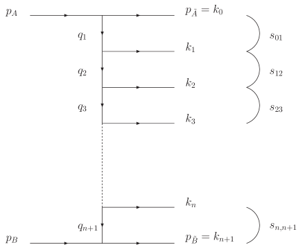
Figure 1: Notation for particle production in MRK.

In MRK the center–of–mass energy for the incoming external particles can be expressed in terms of the internal subenergies as

$$s\simeq\left[\prod_{i=1}^{n+1}s_{i-1,i}\right]\left[\prod_{i=1}^{n}{\bf k}_{i}^{2}\right]^{-1}\simeq\sqrt{{\bf q}_{1}^{2}{\bf q}_{n+1}^{2}}\,\prod_{i=1}^{n+1}\frac{s_{i-1,i}}{\sqrt{{\bf k}_{i-1}^{2}{\bf k}_{i}^{2}}},$$ (3)

where we have used the fact that in Regge kinematics $s$ is much larger than $-t$ and, therefore, $\alpha_{0}\simeq\beta_{n+1}\simeq 1$, ${\bf k}_{0}^{2}\simeq{\bf q}_{1}^{2}$ and ${\bf k}_{n+1}^{2}\simeq{\bf q}_{n+1}^{2}$. To write down the measure of phase space we use dimensional regularization with $D=4+2\,\epsilon$, i.e.

$$ds\;d\Phi_{\tilde{\rm A}\tilde{\rm B}+{\rm n}}=2\pi\prod_{i=1}^{n+1}\frac{ds_{i-1,i}}{2\,s_{i-1,i}}\frac{d^{D-2}{{\bf q}_{i}}\;}{(2\pi)^{D-1}}.$$ (4)

The matrix element $\mathcal{A}_{\tilde{\rm A}\tilde{\rm B}+{\rm n}}$ of Eq. (2) can be written in MRK in the factorized form

$$\frac{\mathcal{A}_{\tilde{\rm A}\tilde{\rm B}+{\rm n}}}{2\,s}=\Gamma_{A}\left[\prod_{i=1}^{n}\frac{1}{q_{i}^{2}}\left(\frac{s_{i-1,i}}{s_{R}}\right)^{\omega_{i}}\gamma(q_{i},q_{i+1})\right]\frac{1}{q_{n+1}^{2}}\left(\frac{s_{n,n+1}}{s_{R}}\right)^{\omega_{n+1}}\Gamma_{B},$$ (5)

with $\Gamma_{P}$ being the couplings of the Reggeon to the external particles, $\omega_{i}=\omega(q_{i}^{2})$ the gluon Regge trajectory depending on the momentum carried by the Reggeon, and $\gamma(q_{i},q_{i+1})$ the gauge invariant effective Reggeon–Reggeon–gluon vertices. At LO the scale $s_{R}$ is a free parameter.

Gathering all these elements together it is possible to write the Mellin transform of Eq. (1) as the sum

$${\cal F}(\omega,s_{0}) = \sum_{n=0}^{\infty}{\cal F}^{(n)}(\omega,s_{0}),$$ (6)

with the contributions from the emission of n $s$–channel gluons being

$$\frac{{\cal F}^{(n)}(\omega,s_{0})}{(2\pi)^{2-D}}=\int\left[\prod_{i=1}^{n+1}d^{D-2}{{\bf q}_{i}}\;\frac{ds_{i-1,i}}{s_{i-1,i}}\left(\frac{s_{i-1,i}}{s_{R}}\right)^{2\omega_{i}}\left(\frac{s_{i-1,i}}{\sqrt{{\bf k}_{i-1}^{2}{\bf k}_{i}^{2}}}\right)^{-\omega}\right]$$ (7)

$$\times\left(\frac{s_{0}}{\sqrt{{\bf q}_{1}^{2}{{\bf q}_{n+1}^{2}}}}\right)^{\omega}\frac{\Phi_{A}({\bf q}_{1})}{{\bf q}_{1}^{2}}\left[\prod_{i=1}^{n}{\cal K}_{r}({\bf q}_{i},{\bf q}_{i+1})\right]\frac{\Phi_{B}({\bf q}_{n+1})}{{\bf q}_{n+1}^{2}}.$$

The impact factors $\Phi_{P}$ and the real emission kernel for Reggeon–Reggeon into a $s$–channel gluon ${\cal K}_{r}$ can be written in terms of the square of the vertices $\Gamma_{P}$ and $\gamma$, respectively. The kernel ${\cal K}_{r}\left({\bf q}_{i},{\bf q}_{i+1}\right)$ is defined such that it includes one gluon propagator on each side: $\left({\bf q}_{i}^{2}{\bf q}^{2}_{i+1}\right)^{-1}$. The integration over $s_{i-1,i}$ in Eq. (7) takes place from a finite $s_{0}$ to infinity. At LO terms of the form $\omega\ln{\bf k}_{i}^{2}$ or $\omega_{i}\ln s_{R}$ can be neglected when the integrand is expanded in $\alpha_{s}$. Therefore, at this accuracy, Eq. (7) gives

$$\frac{{\cal F}^{(n)}(\omega,s_{0})}{(2\pi)^{2-D}}=\int\left[\prod_{i=1}^{n+1}\frac{d^{D-2}{{\bf q}_{i}}\;}{\omega-2\,\omega_{i}}\right]\frac{\Phi_{A}({\bf q}_{1})}{{\bf q}_{1}^{~{}2}}\left[\prod_{i=1}^{n}{\cal K}_{r}({\bf q}_{i},{\bf q}_{i+1})\right]\frac{\Phi_{B}({\bf q}_{n+1})}{{\bf q}_{n+1}^{2}},$$ (8)

where the poles in the complex $\omega$–plane correspond to Reggeon propagators. This simple structure is a consequence of the linearity of the integral equation for the gluon Green’s function. We will see below that Eq. (8) holds very similarly at NLO. This fact has been useful in the study of different NLO BFKL cross sections using numerical techniques in recent years (see Ref. [6]).

After this brief introduction to the structure of BFKL cross sections and its iterative expression we now turn to the NLO case. The factorization into impact factors and Green’s function will remain, while the kernel and trajectory will be more complex than at LO. We discuss these points in the next section.

3 Different contributions at NLO

To discuss the various contributions to NLO BFKL cross sections we follow Ref. [5]. We comment in more detail those points which will turn out to be more relevant for our later discussion of inclusive jet production. Our starting point are Eqs. (1) to (4), which remain unchanged. Since at NLO the $s_{R}$ scale is no longer a free parameter, we should modify Eq. (5) to read

$$\frac{\mathcal{A}_{\tilde{\rm A}\tilde{\rm B}+{\rm n}}}{2\,s} = \Gamma_{A}^{(s_{R;0,1})}\left[\prod_{i=1}^{n}\frac{1}{q_{i}^{2}}\left(\frac{s_{i-1,i}}{s_{R;i-1,i}}\right)^{\omega_{i}}\gamma^{(s_{R;i-1,i},s_{R;i,i+1})}(q_{i},q_{i+1})\right]$$ (9)

$$\hskip 56.9055pt\times\frac{1}{q_{n+1}^{2}}\left(\frac{s_{n,n+1}}{s_{R;n,n+1}}\right)^{\omega_{n+1}}\Gamma_{B}^{(s_{R;n,n+1})}.$$

The propagation of a Reggeized gluon with momentum $q_{i}$ in MRK takes place between two emissions with momenta $k_{i-1}$ and $k_{i}$ (see Fig. 1). Therefore, at NLO, the term $s_{R}$, which scales the invariant energy $s_{i-1,i}$, does depend on these two consecutive emissions and, in general, will be written as $s_{R;i-1,i}$. It is important to note that the production amplitudes should be independent of the energy scale chosen and, therefore,

$$\Gamma_{A}^{(s_{R;0,1})}=\Gamma_{A}^{(s_{R;0,1}^{\prime})}\left(\frac{s_{R;0,1}}{s_{R;0,1}^{\prime}}\right)^{\frac{\omega_{1}}{2}},\,\,\,\,\Gamma_{B}^{(s_{R;n,n+1})}=\Gamma_{B}^{(s_{R;n,n+1}^{\prime})}\left(\frac{s_{R;n,n+1}}{s_{R;n,n+1}^{\prime}}\right)^{\frac{\omega_{n+1}}{2}}$$ (10)

for the particle–particle–Reggeon vertices and

$$\gamma^{(s_{R;i-1,i},s_{R;i,i+1})}\left(q_{i},q_{i+1}\right) = \gamma^{(s_{R;i-1,i}^{\prime},s_{R;i,i+1}^{\prime\prime})}\left(q_{i},q_{i+1}\right)$$ (11)

$$\hskip 28.45274pt\times\left(\frac{s_{R;i-1,i}}{s_{R;i-1,i}^{\prime}}\right)^{\frac{\omega_{i}}{2}}\left(\frac{s_{R;i,i+1}}{s_{R;i,i+1}^{\prime\prime}}\right)^{\frac{\omega_{i+1}}{2}}$$

for the Reggeon–Reggeon–gluon production vertices.

At NLO, besides the two–loop corrections to the gluon Regge trajectory, there are four other contributions which affect the real emission vertex. The first one consists of virtual corrections to the one gluon production vertex. The second stems from the fact that in a chain of emissions widely separated in rapidity two of them are allowed to be nearby in this variable, this is known as quasi–multi–Regge kinematics (QMRK). A third source is obtained by perturbatively expanding the Reggeon propagators in Eq. (9) while keeping MRK and every vertex at LO. A final fourth contribution is that of the production of quark–antiquark pairs. The common feature of all of these new NLO elements is that they generate an extra power in the coupling constant without building up a corresponding logarithm of energy so that $\alpha_{s}\left(\alpha_{s}\ln{s}\right)^{n}$ terms are taken into account.

With the idea of introducing a jet definition later on, it is important to understand the properties of the production vertex which we now describe in some detail.

Lets start with the virtual corrections to the single–gluon emission vertex. These are rather simple and correspond to Eq. (8) with the insertion of a single kernel or impact factor with NLO virtual contributions (noted as ($v$)) while leaving the rest of the expression at Born level (written as ($B$)). More explicitly:

$$\frac{{\cal F}^{(n)}_{\rm virtual}(\omega,s_{0})}{(2\pi)^{2-D}} = \int\left[\prod_{i=1}^{n+1}\frac{d^{D-2}{{\bf q}_{i}}\;}{(\omega-2\omega_{i})}\right]$$ (12)

$$\times\Bigg{\{}\frac{\Phi^{(B)}_{A}({\bf q}_{1})}{{\bf q}_{1}^{2}}\left[\prod_{i=1}^{n}{\cal K}_{r}^{(B)}({\bf q}_{i},{\bf q}_{i+1})\right]\frac{\Phi^{(v)}_{B}({\bf q}_{n+1})}{{\bf q}_{n+1}^{2}}$$

$$+\frac{\Phi^{(v)}_{A}({\bf q}_{1})}{{\bf q}_{1}^{2}}\left[\prod_{i=1}^{n}{\cal K}_{r}^{(B)}({\bf q}_{i},{\bf q}_{i+1})\right]\frac{\Phi^{(B)}_{B}({\bf q}_{n+1})}{{\bf q}_{n+1}^{2}}$$

$$+\frac{\Phi^{(B)}_{A}({\bf q}_{1})}{{\bf q}_{1}^{2}}\sum_{j=1}^{n}\left[\prod_{i=1}^{j-1}{\cal K}_{r}^{(B)}({\bf q}_{i},{\bf q}_{i+1})\right]{\cal K}_{r}^{(v)}({\bf q}_{j},{\bf q}_{j+1})$$

$$\hskip 28.45274pt\times\left[\prod_{i=j+1}^{n}{\cal K}_{r}^{(B)}({\bf q}_{i},{\bf q}_{i+1})\right]\frac{\Phi^{(B)}_{B}({\bf q}_{n+1})}{{\bf q}_{n+1}^{2}}\Bigg{\}}.$$

Now we turn to the discussion of how to define QMRK. For this purpose the introduction of an extra scale is mandatory in order to define a separation in rapidity space between different emissions. As in Ref. [5] we call this new scale $s_{\Lambda}$. At LO MRK implies that all $s_{ij}=(k_{i}+k_{j})^{2}$ are larger than $s_{\Lambda}$. In rapidity space this means that their rapidity difference $|y_{i}-y_{j}|$ is larger than $\ln\frac{s_{\Lambda}}{\sqrt{{\bf k}_{i}^{2}{\bf k}_{j}^{2}}}$. As we stated earlier, in QMRK one single pair of emissions is allowed to be close in rapidity. When any of these two emissions is one of the external particles $\tilde{\rm A}$ or $\tilde{\rm B}$ it contributes as a real correction to the corresponding impact factor. If this is not the case it qualifies as a real correction to the kernel. This is summarized in the following expression where we write real corrections to the impact factors as ($r$):

$$\frac{{\cal F}^{(n+1)}_{\rm QMRK}(\omega,s_{0})}{(2\pi)^{2-D}} = \int\left[\prod_{i=1}^{n+1}\frac{d^{D-2}{{\bf q}_{i}}\;}{(\omega-2\omega_{i})}\right]$$ (13)

$$\times\Bigg{\{}\frac{\Phi^{(B)}_{A}({\bf q}_{1})}{{\bf q}_{1}^{2}}\left[\prod_{i=1}^{n}{\cal K}_{r}^{(B)}({\bf q}_{i},{\bf q}_{i+1})\right]\frac{\Phi^{(r)}_{B}({\bf q}_{n+1})}{{\bf q}_{n+1}^{2}}$$

$$+\frac{\Phi^{(r)}_{A}({\bf q}_{1})}{{\bf q}_{1}^{2}}\left[\prod_{i=1}^{n}{\cal K}_{r}^{(B)}({\bf q}_{i},{\bf q}_{i+1})\right]\frac{\Phi^{(B)}_{B}({\bf q}_{n+1})}{{\bf q}_{n+1}^{2}}$$

$$+\frac{\Phi^{(B)}_{A}({\bf q}_{1})}{{\bf q}_{1}^{2}}\sum_{j=1}^{n}\left[\prod_{i=1}^{j-1}{\cal K}_{r}^{(B)}({\bf q}_{i},{\bf q}_{i+1})\right]{\cal K}_{\rm QMRK}({\bf q}_{j},{\bf q}_{j+1})$$

$$\hskip 28.45274pt\times\left[\prod_{i=j+1}^{n}{\cal K}_{r}^{(B)}({\bf q}_{i},{\bf q}_{i+1})\right]\frac{\Phi^{(B)}_{B}({\bf q}_{n+1})}{{\bf q}_{n+1}^{2}}\Bigg{\}}.$$

The modifications due to QMRK belonging to the kernel or to the impact factors are, respectively, ${\cal K}_{\rm QMRK}$ and $\Phi^{(r)}_{P}$, i.e.

$${\cal K}_{\rm QMRK}({\bf q}_{i},{\bf q}_{i+1}) = (N_{c}^{2}-1)\int d\hat{s}\,\frac{I_{RR}\,\sigma_{RR\rightarrow GG}(\hat{s})\,\theta(s_{\Lambda}-\hat{s})}{(2\pi)^{D}\,{\bf q}_{i}^{2}\,{\bf q}_{i+1}^{2}},$$ (14)

$$\Phi^{(r)}_{P}({\bf k}) = \sqrt{N_{c}^{2}-1}\int d\hat{s}\,\frac{I_{PR}\,\sigma_{PR\rightarrow PG}(\hat{s})\,\theta(s_{\Lambda}-\hat{s})}{(2\pi)\,s}.$$ (15)

In both cases $\hat{s}$ denotes the invariant mass of the two emissions in QMRK. The Heaviside functions are used to separate the regions of phase space where the emissions are at a relative rapidity separation smaller than $s_{\Lambda}$. It is within this region where the LO emission kernel is modified. $\sigma_{RR\rightarrow GG}$ and $\sigma_{PR\rightarrow PG}$ are the total cross sections for two Reggeons into two gluons, and an external particle and a Reggeon into an external particle and a gluon, respectively. $I$ stands for the invariant flux and $N_{c}$ for the number of colours.

For those sectors remaining in the MRK we use a Heaviside function to keep $s_{i-1,i}>s_{\Lambda}$, in this way MRK is clearly separated from QMRK. We then follow the same steps as at LO and use Eq. (7) with the modifications already introduced in Eq. (9), i.e.

$$\frac{{\cal F}_{\rm MRK}^{(n+1)}(\omega,s_{0})}{(2\pi)^{2-D}}$$ (16)

$$=\int\left[\prod_{i=1}^{n+2}d^{D-2}{{\bf q}_{i}}\;\frac{ds_{i-1,i}}{s_{i-1,i}}\left(\frac{s_{i-1,i}}{s_{R;i-1,i}}\right)^{2\omega_{i}}\left(\frac{s_{i-1,i}}{\sqrt{{\bf k}_{i-1}^{2}{\bf k}_{i}^{2}}}\right)^{-\omega}\theta(s_{i-1,i}-s_{\Lambda})\right]$$

$$\times\left(\frac{s_{0}}{\sqrt{{\bf q}_{1}^{2}{\bf q}_{n+2}^{2}}}\right)^{\omega}\frac{\Phi_{A}^{(B)}({\bf q}_{1})}{{\bf q}_{1}^{2}}\left[\prod_{i=1}^{n+1}{\cal K}_{r}^{(B)}({\bf q}_{i},{\bf q}_{i+1})\right]\frac{\Phi_{B}^{(B)}({\bf q}_{n+2})}{{\bf q}_{n+2}^{2}}.$$

After performing the integration over the $s_{i-1,i}$ variables the following interesting dependence on $s_{\Lambda}$ arises:

$$\frac{{\cal F}_{\rm MRK}^{(n+1)}(\omega,s_{0})}{(2\pi)^{2-D}} = \int\left[\prod_{i=1}^{n+2}\frac{d^{D-2}{{\bf q}_{i}}\;}{(\omega-2\omega_{i})}\left(\frac{s_{\Lambda}}{s_{R;i-1,i}}\right)^{2\omega_{i}}\left(\frac{s_{\Lambda}}{\sqrt{{\bf k}_{i-1}^{2}{\bf k}_{i}^{2}}}\right)^{-\omega}\right]$$ (17)

$$\times\left(\frac{s_{0}}{\sqrt{{\bf q}_{1}^{2}{\bf q}_{n+2}^{2}}}\right)^{\omega}\frac{\Phi_{A}^{(B)}({\bf q}_{1})}{{\bf q}_{1}^{2}}\left[\prod_{i=1}^{n+1}{\cal K}_{r}^{(B)}({\bf q}_{i},{\bf q}_{i+1})\right]\frac{\Phi_{B}^{(B)}({\bf q}_{n+2})}{{\bf q}_{n+2}^{2}}.$$

It is now convenient to go back to Eq. (1) and write the lower limit $s_{0}$ of the Mellin transform as a generic product of two scales related to the external impact factors, i.e. $s_{0}=\sqrt{s_{0;A}\,s_{0;B}}$. By expanding in $\alpha_{s}$ the factors with powers in $\omega$ and $\omega_{i}$ it is then possible to identify the NLO terms:

$$\frac{{\cal F}_{\rm MRK}^{(n+1)}(\omega,s_{0})}{(2\pi)^{2-D}}=\int\left[\prod_{i=1}^{n+2}\frac{d^{D-2}{{\bf q}_{i}}\;}{(\omega-2\omega_{i})}\right]\frac{\Phi_{A}^{(B)}({\bf q}_{1})}{{\bf q}_{1}^{2}}\left[\prod_{i=1}^{n+1}{\cal K}_{r}^{(B)}({\bf q}_{i},{\bf q}_{i+1})\right]\frac{\Phi_{B}^{(B)}({\bf q}_{n+2})}{{\bf q}_{n+2}^{2}}$$ (18)

$$\times\Bigg{\{}1-\frac{\omega}{2}\ln\frac{s_{\Lambda}^{2}}{{\bf k}_{1}^{2}s_{0;A}}+\omega_{1}\ln\frac{s_{\Lambda}^{2}}{s_{R;0,1}^{2}}-\sum_{i=2}^{n+1}\left[\frac{\omega}{2}\ln\frac{s_{\Lambda}^{2}}{{\bf k}_{i-1}^{2}{\bf k}_{i}^{2}}-\omega_{i}\ln\frac{s_{\Lambda}^{2}}{s_{R;i-1,i}^{2}}\right]$$

$$\phantom{\times\Bigg{[}1}-\frac{\omega}{2}\ln\frac{s_{\Lambda}^{2}}{{\bf k}_{n+1}^{2}s_{0;B}}+\omega_{n+2}\ln\frac{s_{\Lambda}^{2}}{s_{R;n+1,n+2}^{2}}\Bigg{\}}.$$

To combine this expression with that of the QMRK contribution we should make a choice for $s_{R}$. The most convenient one is $s_{R;i,j}=\sqrt{s_{R;i}\,s_{R;j}}$, where for intermediate Reggeon propagation we use $s_{R;i}={\bf k}_{i}^{2}$, and for the connection with the external particles $s_{R;0}=s_{0;A}$ and $s_{R;n+2}=s_{0;B}$. We can then write

$$\frac{{\cal F}_{\rm MRK}^{(n+1)}(\omega,s_{0})}{(2\pi)^{2-D}}=\int\left[\prod_{i=1}^{n+2}\frac{d^{D-2}{{\bf q}_{i}}\;}{(\omega-2\omega_{i})}\right]\frac{\Phi_{A}^{(B)}({\bf q}_{1})}{{\bf q}_{1}^{2}}\left[\prod_{i=1}^{n+1}{\cal K}_{r}^{(B)}({\bf q}_{i},{\bf q}_{i+1})\right]\frac{\Phi_{B}^{(B)}({\bf q}_{n+2})}{{\bf q}_{n+2}^{2}}$$ (19)

$$\times\Bigg{\{}1-\frac{(\omega-2\omega_{1})}{2}\ln\frac{s_{\Lambda}^{2}}{{\bf k}_{1}^{2}s_{0;A}}-\sum_{i=2}^{n+1}\left[\frac{(\omega-2\omega_{i})}{2}\ln\frac{s_{\Lambda}^{2}}{{\bf k}_{i-1}^{2}{\bf k}_{i}^{2}}\right]$$

$$-\frac{(\omega-2\omega_{n+2})}{2}\ln\frac{s_{\Lambda}^{2}}{{\bf k}_{n+1}^{2}s_{0;B}}\Bigg{\}}.$$

This corresponds to the LO result for ${\cal F}^{(n+1)}$ plus additional terms where the $\omega-2\omega_{i}$ factor cancels, in such a way that they can be combined with the LO result of ${\cal F}^{(n)}$.

The quark contribution can be included in a straightforward manner since between the quark–antiquark emissions there is no propagation of a Reggeized gluon. In this way one can simply write

$$\frac{{\cal F}^{(n+1)}_{Q\bar{Q}}(\omega,s_{0})}{(2\pi)^{2-D}}=\int\left[\prod_{i=1}^{n+1}\frac{d^{D-2}{{\bf q}_{i}}\;}{(\omega-2\omega_{i})}\right]\frac{\Phi^{(B)}_{A}({\bf q}_{1})}{{\bf q}_{1}^{2}}\frac{\Phi^{(B)}_{B}({\bf q}_{n+1})}{{\bf q}_{n+1}^{2}}\\ \times\sum_{j=1}^{n}\left[\prod_{i=1}^{j-1}{\cal K}_{r}^{(B)}({\bf q}_{i},{\bf q}_{i+1})\right]{\cal K}_{Q\bar{Q}}({\bf q}_{j},{\bf q}_{j+1})\left[\prod_{i=j+1}^{n}{\cal K}_{r}^{(B)}({\bf q}_{i},{\bf q}_{i+1})\right].$$ (20)

The production kernel can be written as

$${\cal K}_{Q\bar{Q}}({\bf q}_{i},{\bf q}_{i+1})~{}= ~{}(N_{c}^{2}-1)\int d\hat{s}\,\frac{I_{RR}\,\sigma_{RR\rightarrow Q\bar{Q}}(\hat{s})}{(2\pi)^{D}\,{\bf q}_{i}^{2}\,{\bf q}_{i+1}^{2}},$$ (21)

with $\sigma_{RR\rightarrow Q\bar{Q}}$ being the total cross section for two Reggeons producing the quark–antiquark pair with an invariant mass ${\hat{s}}$.

The combination of all the NLO contributions together generates the following expression for the NLO cross section:

$${\cal F}(\omega,s_{0})_{AB} = \sum_{n=0}^{\infty}\frac{1}{(2\pi)^{D-2}}\int\left[\prod_{i=1}^{n+1}\frac{d^{D-2}{{\bf q}_{i}}\;}{(\omega-2\omega_{i})}\right]$$ (22)

$$\hskip 11.38092pt\times\frac{\Phi_{A}({\bf q}_{1};s_{0;A})}{{\bf q}_{1}^{2}}\left[\prod_{i=1}^{n}{\cal K}_{r}({\bf q}_{i},{\bf q}_{i+1})\right]\frac{\Phi_{B}({\bf q}_{n+1};s_{0;B})}{{\bf q}_{n+1}^{2}},$$

where the NLO real emission kernel contains several terms:

$${\cal K}_{r}({\bf q}_{i},{\bf q}_{i+1}) = \left({\cal K}_{r}^{(B)}+{\cal K}_{r}^{(NLO)}\right)({\bf q}_{i},{\bf q}_{i+1})$$ (23)

$$= \left({\cal K}_{r}^{(B)}+{\cal K}_{r}^{(v)}+{\cal K}_{GG}+{\cal K}_{Q\bar{Q}}\right)({\bf q}_{i},{\bf q}_{i+1}),$$

with ${\cal K}_{Q\bar{Q}}$ given by Eq. (21). The two gluon production kernel ${\cal K}_{GG}$ is the combination of ${\cal K}_{\rm QMRK}$ of Eq. (14) and the MRK contribution in Eq. (19). It explicitly reads

$${\cal K}_{GG}({\bf q}_{i},{\bf q}_{i+1}) = (N_{c}^{2}-1)\int d\hat{s}\frac{I_{RR}\sigma_{RR\rightarrow GG}(\hat{s})\,\theta(s_{\Lambda}-\hat{s})}{(2\pi)^{D}\,{\bf q}_{i}^{2}\,{\bf q}_{i+1}^{2}}$$ (24)

$$-\int d^{D-2}{\tilde{\bf q}}\;\,{\cal K}_{r}^{(B)}({\bf q}_{i},\tilde{\bf q})\,{\cal K}_{r}^{(B)}(\tilde{\bf q},{\bf q}_{i+1})\frac{1}{2}\ln\left(\frac{s_{\Lambda}^{2}}{({\bf q}_{i}-\tilde{\bf q})^{2}({\bf q}_{i+1}-\tilde{\bf q})^{2}}\right).$$

Below we will show that when $s_{\Lambda}$ is taken to infinity the second term of this expression subtracts the logarithmic divergence of the first one. When computing the total cross section it is natural to remove the dependence on the parameter $s_{\Lambda}$ in this way. For our jet production cross section, however, we prefer to retain the dependence upon $s_{\Lambda}$.

For the impact factors a similar expression including virtual and MRK corrections as in Eq. (15) arises:

$$\Phi_{P}({\bf q}_{1};s_{0;P}) = \Phi_{P}^{(B)}+\Phi_{P}^{(v)}+\sqrt{N_{c}^{2}-1}\int d\hat{s}\frac{I_{PR}\,\sigma_{PR}(\hat{s})\,\theta(s_{\Lambda}-\hat{s})}{(2\pi)\,s}$$ (25)

$$-\int d^{D-2}{\tilde{\bf q}}\;\,\Phi^{(B)}_{P}(\tilde{\bf q})\,{\cal K}_{r}^{(B)}(\tilde{\bf q},{\bf q}_{1})\frac{1}{2}\ln\left(\frac{s_{\Lambda}^{2}}{({\bf q}_{1}-\tilde{\bf q})^{2}s_{0;P}}\right).$$

From this expression it is now clear why to choose the factorized form $s_{0}=\sqrt{s_{0;A}\,s_{0;B}}$: in this way each of the impact factors $\Phi_{A,B}$ carry its own $s_{0;A,B}$ term at NLO independently of the choice of scale in the other.

To conclude this section, for the sake of clarity, the different contributions to the NLO BFKL kernel

CONTRIBUTION	NUMBER OF EMISSIONS	Fig.2
MRK @ LO	$n$	(a)
Virtual	$n$	(b)
QMRK	$n+1$	(c)
MRK @ NLO	$n+1$	(d)
Quark–antiquark pair	$n+1$	(e)

are pictorially represented in Fig. 2.

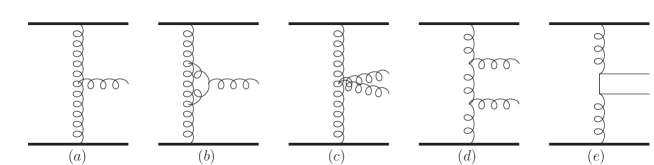
Figure 2: Contributions to real emission kernel at LO (a) and NLO (b-e).

As a final remark we would like to indicate that the divergences present in the gluon trajectories $\omega_{i}$ (see Ref. [2]) are all cancelled inside the inclusive terms. We will see how the soft and collinear divergences of the production vertex are either cancelled amongst its different components or are regularized by the jet definition.

After having introduced the notation and highlighted the different constituents of a BFKL production kernel at NLO, in the coming section we describe how to calculate the inclusive production of jets in two different environments. The first one is the case of the interaction between two small and perturbative objects, highly virtual photons, and the second will be the collision of two large and non–perturbative external particles such as the ones taking place at hadron–hadron colliders.

4 Inclusive jet production at LO

As MRK relies on the transverse scales of the emissions and internal lines being of the same order it is natural to think that processes characterized by two large and similar transverse momenta are the ideal environment for BFKL dynamics to show up. Moreover, as the resummation is based on perturbative degrees of freedom, these large scales associated to the external particles should favor the accuracy of the predictions. An ideal scenario is the interaction between two photons with large virtualities $Q_{1,2}^{2}$ in the Regge limit $s\gg|t|\sim Q_{1}^{2}\sim Q_{2}^{2}$. The total cross section for this process has been investigated in a large number of papers in recent years. Here we are interested in the inclusive production of a single jet in the central region of rapidity in this process. We will consider the case where the transverse momentum of the jet is of the same order as the virtualities of the photons.

As a starting point we review single jet production at LO accuracy. As usual the total cross section can be written as a convolution of the photon impact factors with the gluon Green’s function, i.e.

$$\sigma(s)=\int\frac{d^{2}{\bf k}_{a}}{2\pi{\bf k}_{a}^{2}}\int\frac{d^{2}{\bf k}_{b}}{2\pi{\bf k}_{b}^{2}}\,\Phi_{A}({\bf k}_{a})\,\Phi_{B}({\bf k}_{b})\,\int_{\delta-i\infty}^{\delta+i\infty}\frac{d\omega}{2\pi i}\left(\frac{s}{s_{0}}\right)^{\omega}f_{\omega}({\bf k}_{a},{\bf k}_{b}).$$ (26)

A common choice for the energy scale is $s_{0}=|{\bf k}_{a}|\,|{\bf k}_{b}|$ which naturally introduces the rapidities $y_{\tilde{A}}$ and $y_{\tilde{B}}$ of the emitted particles with momenta $p_{\tilde{A}}$ and $p_{\tilde{B}}$ since

$$\left(\frac{s}{s_{0}}\right)^{\omega}=e^{\omega(y_{\tilde{A}}-y_{\tilde{B}})}.$$ (27)

Let us remark that a change in this scale can be treated as a redefinition of the impact factors and, if $s_{0}$ is chosen to depend only on ${\bf k}_{a}$ or only on ${\bf k}_{b}$, the kernel as well. This treatment lies beyond LO and will be discussed in the next section. The gluon Green’s function $f_{\omega}$ corresponds to the solution of the BFKL equation

$$\omega f_{\omega}({\bf k}_{a},{\bf k}_{b})=\delta^{2}({\bf k}_{a}-{\bf k}_{b})+\int d^{2}{\bf k}\;\mathcal{K}({\bf k}_{a},{\bf k})f_{\omega}({\bf k},{\bf k}_{b}),$$ (28)

$$\mathcal{K}({\bf k}_{a},{\bf k})=2\,\omega({\bf k}_{a}^{2})\,\delta^{2}({\bf k}_{a}-{\bf k})+\mathcal{K}_{r}({\bf k}_{a},{\bf k}),$$ (29)

where the kernel ${\cal K}$ contains a term related to the Reggeized gluon propagator, the trajectory $\omega({\bf k}_{a}^{2})$, and the real emission kernel, ${\cal K}_{r}$.

For the inclusive production of a single jet we assign to it a rapidity $y_{J}$ and a transverse momentum ${\bf k}_{J}$, as shown in Fig. 3. In this way, if $k_{J}=\alpha_{J}p_{A}+\beta_{J}p_{B}+k_{J\perp}$ the corresponding rapidity is $y_{J}=\frac{1}{2}\ln\frac{\alpha_{J}}{\beta_{J}}$. Using its on–shell condition we can write

$$k_{J}=\sqrt{\frac{{\bf k}_{J}^{2}}{s}}e^{y_{J}}p_{A}+\sqrt{\frac{{\bf k}_{J}^{2}}{s}}e^{-y_{J}}p_{B}+k_{J\perp}.$$ (30)

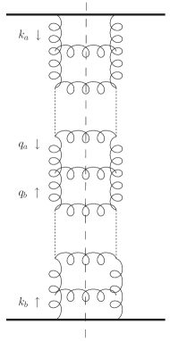
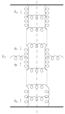
Figure 3: Total cross section and inclusive one jet production in the BFKL approach.

It is possible to single out one gluon emission by extracting its emission probability from the BFKL kernel. The differential cross section in terms of the jet variables can then be constructed in the following way:

$$\frac{d\sigma}{d^{2}{\bf k}_{J}dy_{J}}=\int\frac{d^{2}{\bf k}_{a}}{2\pi{\bf k}_{a}^{2}}\int\frac{d^{2}{\bf k}_{b}}{2\pi{\bf k}_{b}^{2}}\,\Phi_{A}({\bf k}_{a})\,\Phi_{B}({\bf k}_{b})\\ \times\int d^{2}{\bf q}_{a}\int d^{2}{\bf q}_{b}\int_{\delta-i\infty}^{\delta+i\infty}\frac{d\omega}{2\pi i}\left(\frac{s_{AJ}}{s_{0}}\right)^{\omega}f_{\omega}({\bf k}_{a},{\bf q}_{a})\\ \times{\cal V}({\bf q}_{a},{\bf q}_{b};{\bf k}_{J},y_{J})\int_{\delta-i\infty}^{\delta+i\infty}\frac{d\omega^{\prime}}{2\pi i}\left(\frac{s_{BJ}}{s_{0}^{\prime}}\right)^{\omega^{\prime}}f_{\omega^{\prime}}(-{\bf q}_{b},-{\bf k}_{b})$$ (31)

with the LO emission vertex being

$${\cal V}({\bf q}_{a},{\bf q}_{b};{\bf k}_{J},y_{J})=\mathcal{K}_{r}^{(B)}\left({\bf q}_{a},-{\bf q}_{b}\right)\,\delta^{(2)}\left({\bf q}_{a}+{\bf q}_{b}-{\bf k}_{J}\right).$$ (32)

By selecting one emission to be exclusive we have factorized the gluon Green’s function into two components. Each of them connects one of the external particles to the jet vertex. In the notation of Eq. (31) the energies of these blocks are

$$s_{AJ}= (p_{A}+q_{b})^{2}, s_{BJ}= (p_{B}+q_{a})^{2}.$$ (33)

In a symmetric situation, where the jet provides a hard scale as well as the impact factors, a natural choice for the scales is similar to that in the total cross section

$$s_{0}= |{\bf k}_{a}|\,|{\bf k}_{J}|, s_{0}^{\prime}= |{\bf k}_{J}|\,|{\bf k}_{b}|.$$ (34)

These choices can now be related to the relative rapidity between the jet and the external particles. To set the ground for the NLO discussion of the next section we introduce an additional integration over the rapidity $\eta$ of the central system:

$$\frac{d\sigma}{d^{2}{\bf k}_{J}dy_{J}}=\int d^{2}{\bf q}_{a}\int d^{2}{\bf q}_{b}\int d\eta\\ \times\left[\int\frac{d^{2}{\bf k}_{a}}{2\pi{\bf k}_{a}^{2}}\,\Phi_{A}({\bf k}_{a})\,\int_{\delta-i\infty}^{\delta+i\infty}\frac{d\omega}{2\pi i}e^{\omega(y_{A}-\eta)}f_{\omega}({\bf k}_{a},{\bf q}_{a})\right]\,\mathcal{V}({\bf q}_{a},{\bf q}_{b},\eta;{\bf k}_{J},y_{J})\\ \times\left[\int\frac{d^{2}{\bf k}_{b}}{2\pi{\bf k}_{b}^{2}}\,\Phi_{B}({\bf k}_{b})\int_{\delta-i\infty}^{\delta+i\infty}\frac{d\omega^{\prime}}{2\pi i}e^{\omega^{\prime}(\eta-y_{B})}f_{\omega^{\prime}}(-{\bf q}_{b},-{\bf k}_{b})\right]$$ (35)

with the LO emission vertex being

$$\mathcal{V}({\bf q}_{a},{\bf q}_{b},\eta;{\bf k}_{J},y_{J})=\mathcal{K}_{r}^{(B)}\left({\bf q}_{a},-{\bf q}_{b}\right)\,\delta^{(2)}\left({\bf q}_{a}+{\bf q}_{b}-{\bf k}_{J}\right)\,\delta(\eta-y_{J}).$$ (36)

Eqs. (35) and (36) will be the starting point for the NLO jet production in the symmetric configurations.

Let us now switch to the asymmetric case. In general we can write $q_{a}$ and $q_{b}$ as

$$q_{a}= \alpha_{a}p_{A}+\beta_{a}p_{B}+q_{a\perp} q_{b}= \alpha_{b}p_{A}+\beta_{b}p_{B}+q_{b\perp}.$$ (37)

The strong ordering in the rapidity of emissions translates into the conditions $\alpha_{a}\gg\alpha_{b}$ and $\beta_{b}\gg\beta_{a}$. This, together with momentum conservation $q_{a}+q_{b}=k_{J}$, leads us to $\alpha_{J}=\alpha_{a}+\alpha_{b}\approx\alpha_{a}$, $\beta_{J}=\beta_{a}+\beta_{b}\approx\beta_{b}$ and

$$s_{AJ}= \beta_{J}s, s_{BJ}= \alpha_{J}s.$$ (38)

While the longitudinal momentum of $q_{a}(q_{b})$ is a linear combination of $p_{A}$ and $p_{B}$ we see that only its component along $p_{A}(p_{B})$ matters.

If the colliding external particles provide no perturbative scale as it is the case in hadron–hadron collisions, then the jet is the only hard scale in the process and we have to deal with an asymmetric situation. Thus the scales $s_{0}$ and $s_{0}^{\prime}$ should be chosen as ${\bf k}_{J}^{2}$ alone. At LO accuracy $s_{0}$ is arbitrary and we are indeed free to make this choice. Then the arguments of the gluon Green’s functions can be written as

$$\frac{s_{AJ}}{s_{0}}= \frac{1}{\alpha_{a}}, \frac{s_{BJ}}{s_{0}}= \frac{1}{\beta_{b}}.$$ (39)

The description in terms of these longitudinal components is particularly useful if one is interested in jet production in a hadronic environment. Here one can introduce the concept of unintegrated gluon density in the hadron. This represents the probability of resolving a gluon carrying a longitudinal momentum fraction $x$ from the incoming hadron, and with a certain transverse momentum $k_{T}$. With the help of Eq. (39) a LO unintegrated gluon distribution $g$ can be defined from Eq. (31) as

$$g(x,{\bf k})=\int\frac{d^{2}{\bf q}}{2\pi{\bf q}^{2}}\,\Phi_{P}({\bf q})\,\int_{\delta-i\infty}^{\delta+i\infty}\frac{d\omega}{2\pi i}\,x^{-\omega}f_{\omega}({\bf q},{\bf k}).$$ (40)

Then we can rewrite Eq. (31) as

$$\frac{d\sigma}{d^{2}{\bf k}_{J}dy_{J}}=\int d^{2}{\bf q}_{a}\int dx_{1}\int d^{2}{\bf q}_{b}\int dx_{2}\;\\ \times g(x_{1},{\bf q}_{a})g(x_{2},{\bf q}_{b})\mathcal{V}({\bf q}_{a},x_{1},{\bf q}_{b},x_{2};{\bf k}_{J},y_{J}),$$ (41)

with the LO jet vertex for the asymmetric situation being

$$\mathcal{V}({\bf q}_{a},x_{1},{\bf q}_{b},x_{2};{\bf k}_{J},y_{J})=\mathcal{K}_{r}^{(B)}\left({\bf q}_{a},-{\bf q}_{b}\right)\\ \times\delta^{(2)}\left({\bf q}_{a}+{\bf q}_{b}-{\bf k}_{J}\right)\,\delta\left(x_{1}-\sqrt{\frac{{\bf k}_{J}^{2}}{s}}e^{y_{J}}\right)\delta\left(x_{2}-\sqrt{\frac{{\bf k}_{J}^{2}}{s}}e^{-y_{J}}\right).$$ (42)

Having presented our framework for the LO case, in both $\gamma^{*}\gamma^{*}$ and hadron–hadron collisions, we now proceed to explain in detail what corrections are needed to define our cross sections at NLO. Special attention should be put into the treatment of those scales with do not enter the LO discussion but are crucial at higher orders.

5 Inclusive jet production at NLO

A similar approach to that shown in Section 4 remains valid when jet production is considered at NLO. The crucial step in this direction is to modify the LO jet vertex of Eq. (36) and Eq. (42) to include new configurations present at NLO. We show how this is done in the following first subsection. In the second subsection we implement this vertex in the symmetric $\gamma^{*}\gamma^{*}$ case, and we repeat the steps from Eq. (26) to Eq. (38), carefully describing the choice of energy scale at each of the subchannels. In the third subsection hadron–hadron scattering is taken into consideration, and we extend the concept of unintegrated gluon density of Eq. (40) to NLO accuracy. Most importantly, it is shown that a correct choice of intermediate energy scales in this case implies a modification of the impact factors, the jet vertex, and the evolution kernel.

5.1 The NLO jet vertex

For those parts of the NLO kernel responsible for one gluon production we proceed in exactly the same way as at LO. The treatment of those terms related to two particle production is more complicated since for them it is necessary to introduce a jet algorithm. In general terms, if the two emissions generated by the kernel are nearby in phase space they will be considered as one single jet, otherwise one of them will be identified as the jet whereas the other will be absorbed as an untagged inclusive contribution. Hadronization effects in the final state are neglected and we simply define a cone of radius $R_{0}$ in the rapidity–azimuthal angle space such that two particles form a single jet if $R_{12}\equiv\sqrt{(\phi_{1}-\phi_{2})^{2}+(y_{1}-y_{2})^{2}}<R_{0}$. As long as only two emissions are involved this is equivalent to the $k_{T}$–clustering algorithm.

To introduce the jet definition in the $2\rightarrow 2$ components of the kernel it is convenient to start by considering the gluon and quark matrix elements together:

$$\left(\mathcal{K}_{\rm QMRK}+\mathcal{K}_{Q\bar{Q}}\right)({\bf q}_{a},-{\bf q}_{b}) = \int d^{D-2}{{\bf k}_{2}}\int dy_{2}$$ (43)

$$\times\Big{(}\left|\mathcal{A}_{2g}({\bf q}_{a},{\bf q}_{b},{\bf k}_{1},{\bf k}_{2})\right|^{2}\theta(s_{\Lambda}-s_{12})+\left|\mathcal{A}_{2q}({\bf q}_{a},{\bf q}_{b},{\bf k}_{1},{\bf k}_{2})\right|^{2}\Big{)},$$

with ${\cal A}_{2P}$ being the two particle production amplitudes of which only the gluonic one also contributes to MRK. This is why a step function is needed to separate it from MRK. Momentum conservation implies that ${\bf k}_{1}={\bf q}_{a}+{\bf q}_{b}-{\bf k}_{2}$.

The expression (43) is not complete as it stands since we should also include the MRK contribution as it was previously done in Eq. (24):

$$\left({\cal K}_{GG}+{\cal K}_{Q\bar{Q}}\right)({\bf q}_{a},-{\bf q}_{b})\equiv\int d^{D-2}{{\bf k}_{2}}\int dy_{2}\,\left|\mathcal{B}({\bf q}_{a},{\bf q}_{b},{\bf k}_{1},{\bf k}_{2})\right|^{2}$$

$$= \int d^{D-2}{{\bf k}_{2}}\int dy_{2}\,\Bigg{\{}\left|\mathcal{A}_{2g}({\bf q}_{a},{\bf q}_{b},{\bf k}_{1},{\bf k}_{2})\right|^{2}\theta(s_{\Lambda}-s_{12})$$

$$-{\cal K}^{(B)}({\bf q}_{a},{\bf q}_{a}-{\bf k}_{1})\,{\cal K}^{(B)}({\bf q}_{a}-{\bf k}_{1},-{\bf q}_{b})\;\frac{1}{2}\,\theta\left(\ln\frac{s_{\Lambda}}{{\bf k}_{2}^{2}}-y_{2}\right)\theta\left(y_{2}-\ln\frac{{\bf k}_{1}^{2}}{s_{\Lambda}}\right)$$

$$+\left|\mathcal{A}_{2q}({\bf q}_{a},{\bf q}_{b},{\bf k}_{1},{\bf k}_{2})\right|^{2}\Bigg{\}}.$$ (44)

We are now ready to introduce the jet definition for the double emissions. The NLO versions of Eq. (36) and Eq. (42) then read, respectively,

$$\mathcal{V}({\bf q}_{a},{\bf q}_{b},\eta;{\bf k}_{J},y_{J})= \left(\mathcal{K}_{r}^{(B)}+\mathcal{K}_{r}^{(v)}\right)({\bf q}_{a},-{\bf q}_{b})\Big{|}_{(a)}^{[y]}$$

$$+\int d^{D-2}{{\bf k}_{2}}\;dy_{2}\left|\mathcal{B}({\bf q}_{a},{\bf q}_{b},{\bf k}_{J}-{\bf k}_{2},{\bf k}_{2})\right|^{2}\theta(R_{0}-R_{12})\Big{|}_{(b)}^{[y]}$$

$$+2\int d^{D-2}{{\bf k}_{2}}\;dy_{2}\left|\mathcal{B}({\bf q}_{a},{\bf q}_{b},{\bf k}_{J},{\bf k}_{2})\right|^{2}\theta(R_{J2}-R_{0})\Big{|}_{(c)}^{[y]},$$ (45)

$$\mathcal{V}({\bf q}_{a},x_{1},{\bf q}_{b},x_{2};{\bf k}_{J},y_{J})= \left(\mathcal{K}_{r}^{(B)}+\mathcal{K}_{r}^{(v)}\right)({\bf q}_{a},-{\bf q}_{b})\Big{|}_{(a)}^{[x]}$$

$$+\int d^{D-2}{{\bf k}_{2}}\;dy_{2}\left|\mathcal{B}({\bf q}_{a},{\bf q}_{b},{\bf k}_{J}-{\bf k}_{2},{\bf k}_{2})\right|^{2}\theta(R_{0}-R_{12})\Big{|}_{(b)}^{[x]}$$

$$+2\int d^{D-2}{{\bf k}_{2}}\;dy_{2}\left|\mathcal{B}({\bf q}_{a},{\bf q}_{b},{\bf k}_{J},{\bf k}_{2})\right|^{2}\theta(R_{J2}-R_{0})\Big{|}_{(c)}^{[x]}.$$ (46)

In these two expressions we have introduced the notation

$$\Big{|}_{(a,b)}^{[y]} =\delta^{(2)}\left({\bf q}_{a}+{\bf q}_{b}-{\bf k}_{J}\right)\delta(\eta-y^{(a,b)}),$$ (47)

$$\Big{|}_{(c)}^{[y]} =\delta^{(2)}\left({\bf q}_{a}+{\bf q}_{b}-{\bf k}_{J}-{\bf k}_{2}\right)\delta\left(\eta-y^{(c)}\right),$$ (48)

$$\Big{|}_{(a,b)}^{[x]} =\delta^{(2)}\left({\bf q}_{a}+{\bf q}_{b}-{\bf k}_{J}\right)\delta\left(x_{1}-x_{1}^{(a,b)}\right)\delta\left(x_{2}-x_{2}^{(a,b)}\right),$$ (49)

$$\Big{|}_{(c)}^{[x]} =\delta^{(2)}\left({\bf q}_{a}+{\bf q}_{b}-{\bf k}_{J}-{\bf k}_{2}\right)\delta\left(x_{1}-x_{1}^{(c)}\right)\delta\left(x_{2}-x_{2}^{(c)}\right).$$ (50)

The various jet configurations demand different $y$ and $x$ configurations. These are related to the properties of the produced jet in different ways depending on the origin of the jet: if only one gluon was produced in MRK this corresponds to the configuration (a) in the table below, if two particles in QMRK form a jet then we have the case (b), and finally case (c) if the jet is produced out of one of the partons in QMRK. The factor of 2 in the last term of Eq. (45) and Eq. (46) accounts for the possibility that either emitted particle can form the jet. Just by kinematics we get the explicit expressions for the different $x$ configurations listed in the following table:

JET	$y$ configurations	$x$ configurations
a)	$y^{(a)}=y_{J}$	$x_{1}^{(a)}=\frac{|{\bf k}_{J}|}{\sqrt{s}}e^{y_{J}}$	$x_{2}^{(a)}=\frac{|{\bf k}_{J}|}{\sqrt{s}}e^{-y_{J}}$
b)	$y^{(b)}=y_{J}$	$x_{1}^{(b)}=\frac{\sqrt{\Sigma}}{\sqrt{s}}e^{y_{J}}$	$x_{2}^{(b)}=\frac{\sqrt{\Sigma}}{\sqrt{s}}e^{-y_{J}}$
c)	$y^{(c)}=\frac{1}{2}\ln\frac{x_{1}^{(c)}}{x_{2}^{(c)}}$	$x_{1}^{(c)}=\frac{|{\bf k}_{J}|}{\sqrt{s}}e^{y_{J}}+\frac{|{\bf k}_{2}|}{\sqrt{s}}e^{y_{2}}$	$x_{2}^{(c)}=\frac{|{\bf k}_{J}|}{\sqrt{s}}e^{-y_{J}}+\frac{|{\bf k}_{2}|}{\sqrt{s}}e^{-y_{2}}$

The variable $\Sigma$ is defined below in Eq. (58). Due to the analogue treatment of the emission vertex either expressed in terms of rapidities or longitudinal momentum fractions in the remaining of this section we will imply the same analysis for both. In particular, we will not explicitly mention these arguments when we come to Eqs. (68, 69).

The introduction of the jet definition divides the phase space into different sectors. It is now needed to show that the final result is indeed free of any infrared divergences. In the following we proceed to independently calculate several contributions to the kernel to be able, in this way, to study its singularity structure.

The NLO virtual correction to the one–gluon emission kernel, ${\cal K}^{(v)}$, was originally calculated in Ref. [7, 8, 9]. Its expression reads

$$\mathcal{K}_{r}^{(v)}\left({\bf q}_{a},-{\bf q}_{b}\right) = \frac{\bar{g}_{\mu}^{4}\mu^{-2\epsilon}}{\pi^{1+\epsilon}\Gamma(1-\epsilon)}\frac{4}{{\bf{\Delta}}^{2}}\Bigg{\{}2\left(\frac{{\bf{\Delta}}^{2}}{\mu^{2}}\right)^{\epsilon}\left(-\frac{1}{\epsilon^{2}}+\frac{\pi^{2}}{2}-2\,\epsilon\,\zeta(3)\right)$$ (51)

$$+\frac{\beta_{0}}{N_{c}}\frac{1}{\epsilon}+\,\frac{3{\bf{\Delta}}^{2}}{{\bf q}_{a}^{2}-{\bf q}_{b}^{2}}\ln\left(\frac{{\bf q}_{a}^{2}}{{\bf q}_{b}^{2}}\right)-\ln^{2}\left(\frac{{\bf q}_{a}^{2}}{{\bf q}_{b}^{2}}\right)$$

$$+\,\left(1-\frac{n_{f}}{N_{c}}\right)\bigg{[}\frac{{\bf{\Delta}}^{2}}{{\bf q}_{a}^{2}-{\bf q}_{b}^{2}}\left(1-\frac{{\bf{\Delta}}^{2}({\bf q}_{a}^{2}+{\bf q}_{b}^{2}-4\,{\bf q}_{a}{\bf q}_{b})}{3({\bf q}_{a}^{2}-{\bf q}_{b}^{2})^{2}}\right)\ln\left(\frac{{\bf q}_{a}^{2}}{{\bf q}_{b}^{2}}\right)$$

$$-\,\frac{{\bf{\Delta}}^{2}}{6{\bf q}_{a}^{2}{\bf q}_{b}^{2}}({\bf q}_{a}-{\bf q}_{b})^{2}+\frac{{\bf{\Delta}}^{4}\,({\bf q}_{a}^{2}+{\bf q}_{b}^{2})}{6{\bf q}_{a}^{2}{\bf q}_{b}^{2}({\bf q}_{a}^{2}-{\bf q}_{b}^{2})^{2}}({\bf q}_{a}^{2}+{\bf q}_{b}^{2}-4\,{\bf q}_{a}{\bf q}_{b})\bigg{]}\Bigg{\}},$$

with $\beta_{0}=(11N_{c}-2n_{f})/3$, $\zeta(n)=\sum_{k=1}^{\infty}k^{-n}$ and ${\bf\Delta}={\bf q}_{a}+{\bf q}_{b}$. ${\bar{g}}_{\mu}$ can be expressed in terms of the renormalized coupling constant $g_{\mu}$ in the $\overline{\rm MS}$ renormalization scheme by the relation $\bar{g}_{\mu}^{2}=g_{\mu}^{2}\,N_{c}\,\Gamma(1-\epsilon)\,(4\pi)^{-2-\epsilon}$. Note that the expression for the virtual contribution given in [4] lacks the log squared.

Those pieces related to two–gluon production in QMRK can be rewritten in terms of their corresponding matrix elements as

$$\mathcal{K}_{\rm QMRK}({\bf q}_{a},-{\bf q}_{b}) = \int d^{D-2}{{\bf k}_{2}}\int dy_{2}\left|\mathcal{A}_{2g}({\bf q}_{a},{\bf q}_{b},{\bf k}_{1},{\bf k}_{2})\right|^{2}\theta(s_{\Lambda}-s_{12})$$ (52)

$$=\frac{g_{\mu}^{2}\mu^{-2\epsilon}N_{c}^{2}}{\pi(2\pi)^{D+1}{\bf q}_{a}^{2}{\bf q}_{b}^{2}}\int\frac{d^{D-2}{{\bf k}_{2}}}{\mu^{2\epsilon}(2\pi)^{D-4}}\int dy_{2}\;A_{\text{gluons}}\,\theta(s_{\Lambda}-s_{12}),$$

and those related to quark–antiquark production are

$$\mathcal{K}_{Q\bar{Q}}({\bf q}_{a},-{\bf q}_{b}) = \int d^{D-2}{{\bf k}_{2}}\int dy_{2}\left|\mathcal{A}_{2q}({\bf q}_{a},{\bf q}_{b},{\bf k}_{1},{\bf k}_{2})\right|^{2}$$ (53)

$$= \frac{g_{\mu}^{2}\mu^{-2\epsilon}N_{c}^{2}}{\pi(2\pi)^{D+1}{\bf q}_{a}^{2}{\bf q}_{b}^{2}}\int\frac{d^{D-2}{{\bf k}_{2}}}{\mu^{2\epsilon}(2\pi)^{D-4}}\int dy_{2}\;A_{\text{quarks}}.$$

We have calculated the corresponding amplitudes, using the Mandelstam invariants $\hat{s}$, $\hat{t}$, and $\hat{u}$, and our results are

$$A_{\text{gluons}} = {\bf q}_{a}^{2}{\bf q}_{b}^{2}\Bigg{\{}-\frac{1}{\hat{t}\hat{u}}+\frac{1}{4\hat{t}\hat{u}}\frac{{\bf q}_{a}^{2}{\bf q}_{b}^{2}}{{\bf k}_{1}^{2}{\bf k}_{2}^{2}}-\frac{1}{4}\left(\frac{1-x}{x}\frac{1}{{\bf k}_{2}^{2}\hat{t}}+\frac{x}{1-x}\frac{1}{{\bf k}_{1}^{2}\hat{u}}\right)+\frac{1}{4{\bf k}_{1}^{2}{\bf k}_{2}^{2}}$$ (54)

$$\hskip 2.84544pt+\frac{1}{\Sigma}\Bigg{[}-\frac{1}{\hat{s}}\left(2+\left(\frac{1}{\hat{t}}-\frac{1}{\hat{u}}\right)\left(\frac{1-x}{x}{\bf k}_{1}^{2}-\frac{x}{1-x}{\bf k}_{2}^{2}\right)\right)+\frac{1}{4}\left(\frac{\Sigma}{\hat{s}}+1\right)$$

$$\hskip 28.45274pt\times\left(\frac{1-x}{x}\frac{1}{{\bf k}_{2}^{2}}+\frac{x}{1-x}\frac{1}{{\bf k}_{1}^{2}}\right)-\frac{{\bf q}_{b}^{2}}{4\hat{s}}\left(\frac{1}{(1-x)\hat{t}}+\frac{1}{x\hat{u}}\right)$$

$$\hskip 28.45274pt-\frac{{\bf q}_{a}^{2}}{4\hat{s}}\left(\left[1+\frac{x}{1-x}\frac{{\bf k}_{2}^{2}}{{\bf k}_{1}^{2}}\right]\frac{1}{\hat{t}}+\left[1+\frac{1-x}{x}\frac{{\bf k}_{1}^{2}}{{\bf k}_{2}^{2}}\right]\frac{1}{\hat{u}}\right)\Bigg{]}\Bigg{\}}$$

$$+ \frac{D-2}{4}\Bigg{\{}\left(\frac{({\bf k}_{1}-{\bf q}_{a})^{2}({\bf k}_{2}-{\bf q}_{a})^{2}-{\bf k}_{1}^{2}{\bf k}_{2}^{2}}{\hat{t}\hat{u}}\right)^{2}$$

$$-\frac{1}{4}\left(\frac{({\bf k}_{2}-{\bf q}_{a})^{2}-\frac{x}{1-x}{\bf k}_{2}^{2}}{\hat{u}}+\frac{E}{\hat{s}}\right)\left(\frac{({\bf k}_{1}-{\bf q}_{a})^{2}-\frac{1-x}{x}{\bf k}_{1}^{2}}{\hat{t}}-\frac{E}{\hat{s}}\right)\Bigg{\}},$$

$$A_{\text{quarks}} = \frac{n_{f}}{4N_{c}}\Bigg{\{}\frac{{\bf q}_{a}^{2}{\bf q}_{b}^{2}}{\hat{s}\Sigma}\left(2+\left(\frac{1}{\hat{t}}-\frac{1}{\hat{u}}\right)\left(\frac{1-x}{x}{\bf k}_{1}^{2}-\frac{x}{1-x}{\bf k}_{2}^{2}\right)\right)$$ (55)

$$-\left(\frac{({\bf k}_{1}-{\bf q}_{a})^{2}({\bf k}_{2}-{\bf q}_{a})^{2}-{\bf k}_{1}^{2}{\bf k}_{2}^{2}}{\hat{t}\hat{u}}\right)^{2}$$

$$+\frac{1}{2}\left(\frac{({\bf k}_{2}-{\bf q}_{a})^{2}-\frac{x}{1-x}{\bf k}_{2}^{2}}{\hat{u}}+\frac{E}{\hat{s}}\right)\left(\frac{({\bf k}_{1}-{\bf q}_{a})^{2}-\frac{1-x}{x}{\bf k}_{1}^{2}}{\hat{t}}-\frac{E}{\hat{s}}\right)\Bigg{\}}$$

$$+\frac{n_{f}}{4N_{c}^{3}}\Bigg{\{}\left(\frac{({\bf k}_{1}-{\bf q}_{a})^{2}({\bf k}_{2}-{\bf q}_{a})^{2}-{\bf k}_{1}^{2}{\bf k}_{2}^{2}}{\hat{t}\hat{u}}\right)^{2}-\frac{{\bf q}_{a}^{2}{\bf q}_{b}^{2}}{\hat{t}\hat{u}}\Bigg{\}}.$$

These expressions are in agreement with the corresponding ones obtained in Ref. [4]. The following notation has been used:

$$x = \frac{|{\bf k}_{1}|}{|{\bf k}_{1}|+|{\bf k}_{2}|e^{\Delta y}},$$ (56)

$${\bf{\Lambda}} = (1-x){\bf k}_{1}-x{\bf k}_{2},$$ (57)

$$\Sigma = \hat{s}+{\bf{\Delta}}^{2}\,=\,\frac{{\bf{\Lambda}}^{2}}{x(1-x)}+{\bf\Delta}^{2},$$ (58)

$$E = 2(2x-1){\bf q}_{a}^{2}+4{\bf{\Lambda}}{\bf q}_{a}+\frac{1-2x}{x(1-x)}{\bf{\Lambda}}^{2}$$ (59)

$$- 2x(1-x)\left((2x-1){\bf{\Delta}}^{2}+2{\bf{\Lambda}}{\bf{\Delta}}\right)\frac{{\bf q}_{a}^{2}}{x(1-x){\bf{\Delta}}^{2}+{\bf{\Lambda}}^{2}}.$$

We now study those terms which contribute to generate soft and collinear divergences after integration over the two–particle phase space. They should be able to cancel the $\epsilon$ poles of the virtual contributions in Eq. (51), i.e.

$$\mathcal{K}^{(v)}_{\rm singular}\left({\bf q}_{a},{\bf q}_{b}\right) = \frac{\bar{g}_{\mu}^{4}\mu^{-2\epsilon}}{\pi^{1+\epsilon}\Gamma(1-\epsilon)}\frac{4}{{\bf{\Delta}}^{2}}\Bigg{\{}\left(\frac{{\bf{\Delta}}^{2}}{\mu^{2}}\right)^{\epsilon}\left(-\frac{2}{\epsilon^{2}}\right)+\frac{\beta_{0}}{N_{c}}\frac{1}{\epsilon}\Bigg{\}}.$$ (60)

Here we identify those pieces responsible for the generation of these poles.

One of the divergent regions is defined by the two emissions with momenta $k_{1}=\alpha_{1}p_{A}+\beta_{1}p_{B}+k_{1\perp}$ and $k_{2}=\alpha_{2}p_{A}+\beta_{2}p_{B}+k_{2\perp}$ becoming collinear. This means that, for a real parameter $\lambda$, $k_{1}\simeq\lambda\,k_{2}$, i.e. $k_{1\perp}\simeq\lambda\,k_{2\perp}$, $\alpha_{1}\simeq\lambda\,\alpha_{2}$ and thus $\alpha_{2}k_{1\perp}-\alpha_{1}k_{2\perp}\simeq 0$. Since $x=\frac{\alpha_{1}}{\alpha_{1}+\alpha_{2}}$ this is equivalent to the condition ${\bf{\Lambda}}\simeq 0$. In the collinear region $\hat{s}=\frac{{\bf{\Lambda}}^{2}}{x(1-x)}$ tends to zero and the dominant contributions which are purely collinear are

$$A_{\text{gluons}}^{\text{singular}}\Big{|}_{\rm collinear}= -\frac{{\bf q}_{a}^{2}{\bf q}_{b}^{2}}{\Sigma}\frac{2}{\hat{s}}+\frac{D-2}{16}\frac{E^{2}}{\hat{s}^{2}}\equiv A_{(1)}+A_{(2)},$$ (61)

$$A_{\text{quarks}}^{\text{singular}}\Big{|}_{\rm collinear}= \frac{n_{f}}{2N_{c}}\frac{{\bf q}_{a}^{2}{\bf q}_{b}^{2}}{\hat{s}\Sigma}-\frac{n_{f}}{8N_{c}}\frac{E^{2}}{\hat{s}^{2}}.$$ (62)

The quark–antiquark production does not generate divergences when ${\bf k}_{1}$ or ${\bf k}_{2}$ become soft, therefore we have that the only purely soft divergence is

$$A_{\text{gluons}}^{\text{singular}}\Big{|}_{\rm soft}={\bf q}_{a}^{2}{\bf q}_{b}^{2}\Bigg{(}\frac{1}{4\hat{t}\hat{u}}\frac{{\bf q}_{a}^{2}{\bf q}_{b}^{2}}{{\bf k}_{1}^{2}{\bf k}_{2}^{2}}+\frac{1}{4{\bf k}_{1}^{2}{\bf k}_{2}^{2}}\Bigg{)}\equiv A_{(3)}+A_{(4)}~{}\rightarrow~{}2A_{(4)},$$ (63)

where we have used the property that, in the soft limit, the $\hat{t}\hat{u}$ product tends to ${\bf q}_{a}^{2}{\bf q}_{b}^{2}$. We will see that these terms will be responsible for simple poles in $\epsilon$. The double poles will be generated by the regions with simultaneous soft and collinear divergences. They are only present in the gluon–gluon production case and can be written as

$$A_{\text{gluons}}^{\text{singular}}\Big{|}_{\rm soft\&collinear} = \frac{{\bf q}_{a}^{2}{\bf q}_{b}^{2}}{4\hat{s}}\left[\frac{1-x}{x}\frac{1}{{\bf k}_{2}^{2}}+\frac{x}{1-x}\frac{1}{{\bf k}_{1}^{2}}\right]$$ (64)

$$-\frac{{\bf q}_{a}^{2}{\bf q}_{b}^{2}}{4\hat{s}\Sigma}\Bigg{[}{\bf q}_{b}^{2}\left(\frac{1}{(1-x)\hat{t}}+\frac{1}{x\hat{u}}\right)+{\bf q}_{a}^{2}\left(\left[1+\frac{x}{1-x}\frac{{\bf k}_{2}^{2}}{{\bf k}_{1}^{2}}\right]\frac{1}{\hat{t}}+\left[1+\frac{1-x}{x}\frac{{\bf k}_{1}^{2}}{{\bf k}_{2}^{2}}\right]\frac{1}{\hat{u}}\right)\Bigg{]}.$$

$$= A_{(5)}+A_{(6)}.$$

Focusing on the divergent structure it turns out that in the soft and collinear region the first line of Eq. (64), $A_{(5)}$, has exactly the same limit as the second line, $A_{(6)}$. This is very convenient since we can then simply write

$$A_{\text{gluons}}^{\text{singular}}\Big{|}_{\rm soft\&collinear} \rightarrow \frac{{\bf q}_{a}^{2}{\bf q}_{b}^{2}}{2\hat{s}}\left(\frac{1-x}{x}\frac{1}{{\bf k}_{2}^{2}}+\frac{x}{1-x}\frac{1}{{\bf k}_{1}^{2}}\right)=2A_{(5)}.$$ (65)

The MRK contribution of Eq. (44) has the form $A_{\rm MRK}=-4A_{(4)}$ and when added to all the other singular terms we get the expression

$$\int d^{D-2}{{\bf k}_{2}}\int dy_{2}\,\left|\mathcal{B}_{s}({\bf q}_{a},{\bf q}_{b},{\bf k}_{2},{\bf k}_{1})\right|^{2} \equiv$$ (66)

$$\frac{g_{\mu}^{2}\mu^{-2\epsilon}N_{c}^{2}}{\pi(2\pi)^{D+1}{\bf q}_{a}^{2}{\bf q}_{b}^{2}}\int\frac{d^{D-2}{{\bf k}_{2}}}{\mu^{2\epsilon}(2\pi)^{D-4}}\int dy_{2}\,\Big{\{}A^{\rm singular}_{\text{gluons}}\,\theta(s_{\Lambda}-s_{12})+A^{\rm singular}_{\text{quarks}}\Big{\}},$$

with

$$A^{\rm singular}_{\text{gluons}}\,\theta(s_{\Lambda}-s_{12})+A^{\rm singular}_{\text{quarks}} =$$ (67)

$$\left\{\underbrace{-\frac{{\bf q}_{a}^{2}{\bf q}_{b}^{2}}{\Sigma}\frac{2}{\hat{s}}}_{\rm Gluon|_{coll_{1}}}+\underbrace{\frac{D-2}{16}\frac{E^{2}}{\hat{s}^{2}}}_{\rm Gluon|_{coll_{2}}}-\underbrace{\frac{{\bf q}_{a}^{2}{\bf q}_{b}^{2}}{2{\bf k}_{1}^{2}{\bf k}_{2}^{2}}}_{\rm Gluon|_{soft}}+\underbrace{\frac{{\bf q}_{a}^{2}{\bf q}_{b}^{2}}{2\hat{s}}\left(\frac{1-x}{x}\frac{1}{{\bf k}_{2}^{2}}+\frac{x}{1-x}\frac{1}{{\bf k}_{1}^{2}}\right)}_{\rm Gluon|_{\rm soft\&coll}}\right\}\theta(s_{\Lambda}-s_{12})$$

$$+\underbrace{\frac{n_{f}}{2N_{c}}\frac{{\bf q}_{a}^{2}{\bf q}_{b}^{2}}{\hat{s}\Sigma}}_{\rm Quark|_{coll_{1}}}-\underbrace{\frac{n_{f}}{8N_{c}^{3}}\frac{E^{2}}{\hat{s}^{2}}}_{\rm Quark|_{coll_{2}}}..$$

We have labeled the different terms to study how each of them produces the $\epsilon$ poles. We will do this in Section 6.

With the singularity structure well identified we now come back to Eqs. (45, 46) and show how they are free of any divergences. Only if the divergent terms belong to the same configuration this cancellation can be shown analytically. With this in mind we add the singular parts of the two particle production of Eq. (66) in the configuration $(a)$ multiplied by $0=1-\theta(R_{0}-R_{12})-\theta(R_{12}-R_{0})$:

$$\mathcal{V} = \bigg{[}\left(\mathcal{K}_{r}^{(B)}+\mathcal{K}_{r}^{(v)}\right)({\bf q}_{a},-{\bf q}_{b})$$ (68)

$$\hskip 85.35826pt+\int d^{D-2}{{\bf k}_{2}}\;dy_{2}\left|\mathcal{B}_{s}({\bf q}_{a},{\bf q}_{b},{\bf k}_{J}-{\bf k}_{2},{\bf k}_{2})\right|^{2}\bigg{]}\Big{|}_{(a)}$$

$$+ \int d^{D-2}{{\bf k}_{2}}\;dy_{2}\bigg{[}\left|\mathcal{B}({\bf q}_{a},{\bf q}_{b},{\bf k}_{J}-{\bf k}_{2},{\bf k}_{2})\right|^{2}\Big{|}_{(b)}$$

$$\hskip 85.35826pt-\left|\mathcal{B}_{s}({\bf q}_{a},{\bf q}_{b},{\bf k}_{J}-{\bf k}_{2},{\bf k}_{2})\right|^{2}\Big{|}_{(a)}\bigg{]}\theta(R_{0}-R_{12})$$

$$+ \bigg{[}2\int d^{D-2}{{\bf k}_{2}}\;dy_{2}\left|\mathcal{B}({\bf q}_{a},{\bf q}_{b},{\bf k}_{J},{\bf k}_{2})\right|^{2}\theta(R_{J2}-R_{0})\Big{|}_{(c)}$$

$$\hskip 11.38092pt-\int d^{D-2}{{\bf k}_{2}}\;dy_{2}\left|\mathcal{B}_{s}({\bf q}_{a},{\bf q}_{b},{\bf k}_{J}-{\bf k}_{2},{\bf k}_{2})\right|^{2}\theta(R_{12}-R_{0})\Big{|}_{(a)}\bigg{]}.$$

The cancellation of divergences within the first two lines is now the same as in the calculation of the full NLO kernel. In Section 6 we will show how the first two lines of Eq. (68) are free of any singularities in the form of $\epsilon$ poles. In doing so we will go into the details of the rôle of $s_{\Lambda}$. The third and fourth lines are also explicitly free of divergences since these have been subtracted out. The sixth line has a ${\bf k}_{1}\leftrightarrow{\bf k}_{2}$ symmetry which allows us to write

$$\mathcal{V} = \bigg{[}\left(\mathcal{K}_{r}^{(B)}+\mathcal{K}_{r}^{(v)}\right)({\bf q}_{a},-{\bf q}_{b})$$ (69)

$$\hskip 85.35826pt+\int d^{D-2}{{\bf k}_{2}}\;dy_{2}\left|\mathcal{B}_{s}({\bf q}_{a},{\bf q}_{b},{\bf k}_{J}-{\bf k}_{2},{\bf k}_{2})\right|^{2}\bigg{]}\Big{|}_{(a)}$$

$$+ \int d^{D-2}{{\bf k}_{2}}\;dy_{2}\bigg{[}\left|\mathcal{B}({\bf q}_{a},{\bf q}_{b},{\bf k}_{J}-{\bf k}_{2},{\bf k}_{2})\right|^{2}\Big{|}_{(b)}$$

$$\hskip 85.35826pt-\left|\mathcal{B}_{s}({\bf q}_{a},{\bf q}_{b},{\bf k}_{J}-{\bf k}_{2},{\bf k}_{2})\right|^{2}\Big{|}_{(a)}\bigg{]}\theta(R_{0}-R_{12})$$

$$+ 2\int d^{D-2}{{\bf k}_{2}}\;dy_{2}\bigg{[}\left|\mathcal{B}({\bf q}_{a},{\bf q}_{b},{\bf k}_{J},{\bf k}_{2})\right|^{2}\theta(R_{J2}-R_{0})\Big{|}_{(c)}$$

$$\hskip 11.38092pt-\left|\mathcal{B}_{s}({\bf q}_{a},{\bf q}_{b},{\bf k}_{J}-{\bf k}_{2},{\bf k}_{2})\right|^{2}\theta(R_{12}-R_{0})\theta(|{\bf k}_{1}|-|{\bf k}_{2}|)\Big{|}_{(a)}\bigg{]}.$$

We can now see that the remaining possible divergent regions of the last line are regulated by the cone radius $R_{0}$.

It is worth noting that, apart from an overall ${\bar{\alpha}}_{s}^{2}(\mu^{2})$ factor, the NLO terms in the last four lines in Eq. (69) do not carry any renormalization scale dependence since they are finite when $\epsilon$ is set to zero. The situation is different for the first two lines since $\mathcal{V}$ contains a logarithm of $\mu^{2}$ in the form

$$\mathcal{V}=\mathcal{V}^{(B)}\left(1-\frac{\alpha_{s}(\mu^{2})}{4\pi}\frac{\beta_{0}}{N_{c}}\ln\frac{{\bf k}_{J}^{2}}{\mu^{2}}\right)+\Delta\mathcal{V}.$$ (70)

where $\Delta\mathcal{V}$ contains the third to sixth lines and the $\mu$–independent part of the first two lines of (69). It is then natural to absorb this term in a redefinition of the running of the coupling and replace $\alpha_{s}(\mu^{2})$ by $\alpha_{s}({\bf k}_{J}^{2})$. For a explicit derivation of this term we refer the reader to Section 6.

Therefore we now have a finite expression for the jet vertex suitable for numerical integration. This numerical analysis will be performed elsewhere since here we are mainly concerned with the formal introduction of the jet definition and the correct separation of the different contributions to the kernel.

What remains to be proven is the cancellation of divergences between Eq. (60) and Eq. (66). This will be performed in Section 6. Before doing so, in the next two subsections, we indicate how to introduce our vertex in the definition of the differential cross section. Especial care must be taken in the treatment of the energy scale in the Reggeized gluon propagators since in the symmetric case it is directly related to the rapidity difference between subsequent emissions, as we will show in the next subsection, but in the asymmetric case of hadron–hadron collisions it depends on the longitudinal momentum fractions of the $t$–channel Reggeons.

5.2 Production of jets in $\gamma^{*}\gamma^{*}$ scattering

We now have all the ingredients required to describe the inclusive single jet production in a symmetric process at NLO. To be definite, we consider $\gamma^{*}\gamma^{*}$ scattering with the virtualities of the two photons being large and of the same order. All we need is to take Eq. (31) for the differential cross section as a function of the transverse momentum and rapidity of the jet. The vertex ${\cal V}$ to be used is that of Eq. (69) in the representation based on rapidity variables of Eq. (45). The rapidities of the emitted particles are the natural variables to characterize the partonic evolution and $s$–channel production since we assume that all transverse momenta are of the same order.

Let us note that the rapidity difference between two emissions can be written as

$$y_{i}-y_{i+1} = \ln{\frac{s_{i,i+1}}{\sqrt{{\bf k}_{i}^{2}{\bf k}_{i+1}^{2}}}}$$ (71)

which supports the choice $s_{R;i,i+1}=\sqrt{{\bf k}_{i}^{2}{\bf k}_{i+1}^{2}}$ in Eq. (9). This is also technically more convenient since it simplifies the final expression for the cross section in Eq. (19).

In Fig. 4 we illustrate the different scales participating in the scattering and the variables of evolution. We write down the conditions for MRK: all transverse momenta are of similar size and much larger than the confining scale, the rapidities are strongly ordered in the evolution from one external particle to the other. At each stage of the evolution the propagation of the Reggeized gluons, which generates rapidity gaps, takes place between two real emissions. There are many configurations contributing to the differential cross section, each of them with a different weight. Eq. (31) represents the sum of these production processes.

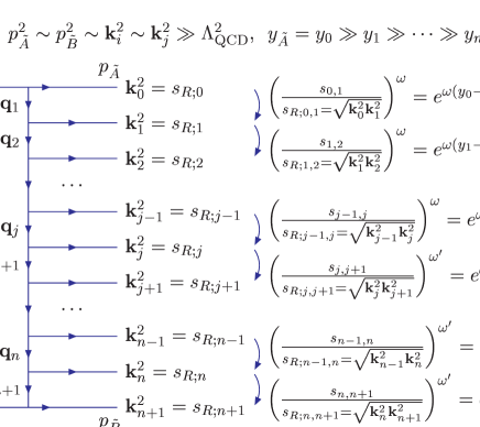
Figure 4: Momenta for $2\rightarrow 2+(n-1)+{\rm jet}$ amplitude in the symmetric configuration with MRK. The produced jet has rapidity $y_{J}=y_{j}$ and transverse momentum ${\bf k}_{J}={\bf k}_{j}$.

5.3 The unintegrated gluon density and jet production in hadron–hadron collisions

In this subsection we now turn to the case of hadron collisions where MRK has to be necessarily modified to include some evolution in the transverse momenta, since the momentum of the jet will be much larger than the typical transverse scale associated to the hadron.

In the LO case we have already explained that, in order to move from the symmetric case to the asymmetric one, it is needed to change the energy scale from Eq. (34) to Eq. (39). This is equivalent to changing the description of the evolution in terms of rapidity differences between emissions to longitudinal momentum fractions of the Reggeized gluons in the $t$–channel. Whereas in LO this change of scales has no consequences, in NLO accuracy it leads to modifications, not only of the jet emission vertex but also of the evolution kernels above and below the jet vertex.

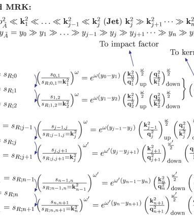
Figure 5: Momenta for $2\rightarrow 2+(n-1)+{\rm jet}$ amplitude in the asymmetric configuration with $k_{t}$–ordered MRK.

These new definitions will allow the cross section still to be written in a factorizable way and the evolution of the gluon Green’s function still to be described by an integral equation.

To understand this in detail we start by writing the solution to the NLO BFKL equation iteratively, i.e.

$$\int d^{2}{\bf k}_{a}f_{\omega}({\bf k}_{a},{\bf q}_{a}) = \frac{1}{\omega}\sum_{j=1}^{\infty}\left[\prod_{i=1}^{j-1}\int d^{2}{\bf q}_{i}\frac{1}{\omega}\mathcal{K}({\bf q}_{i},{\bf q}_{i+1})\right],$$ (72)

where ${\bf q}_{1}={\bf k}_{a}$ and ${\bf q}_{j}={\bf q}_{a}$. We now focus on one side of the evolution towards the hard scale since the other side is similar and use Fig. 5 as a graphical reference. Starting with the symmetric case the differential cross section for jet production contains the following evolution between particle $A$ and the jet:

$$\frac{d\sigma}{d^{2}{\bf k}_{J}dy_{J}} = \int d^{2}{\bf q}_{a}\int d^{2}{\bf k}_{a}\frac{\Phi_{A}({\bf k}_{a})}{2\pi{\bf k}_{a}^{2}}$$ (73)

$$\hskip 2.84544pt\times\int\frac{d\omega}{2\pi i}f_{\omega}({\bf k}_{a},{\bf q}_{a})\left(\frac{s_{AJ}}{\sqrt{{\bf k}_{a}^{2}{\bf k}_{J}^{2}}}\right)^{\omega}{\cal V}({\bf q}_{a},{\bf q}_{b};{\bf k}_{J},y_{J})\dots$$

In the asymmetric situation where ${\bf k}_{J}^{2}\gg{\bf k}_{a}^{2}$ the scale $\sqrt{{\bf k}_{a}^{2}{\bf k}_{J}^{2}}$ should be replaced by ${\bf k}_{J}^{2}$. In order to do so we rewrite the term related to the choice of energy scale. To be consistent with Fig. 5 we take ${\bf k}_{j}={\bf k}_{J}$, ${\bf k}_{0}=-{\bf k}_{a}=-{\bf q}_{1}$ and ${\bf q}_{j}={\bf q}_{a}$. To start with it is convenient to introduce a chain of scale changes in every kernel:

$$\left(\frac{s_{AJ}}{\sqrt{{\bf k}_{a}^{2}{\bf k}_{J}^{2}}}\right)^{\omega} = \left[\prod_{i=1}^{j}\left(\frac{{\bf k}_{i}^{2}}{{\bf k}_{i-1}^{2}}\right)^{\frac{\omega}{2}}\right]\left(\frac{s_{AJ}}{{\bf k}_{J}^{2}}\right)^{\omega},$$ (74)

which can alternatively be written in terms of the $t$–channel momenta as

$$\left(\frac{s_{AJ}}{\sqrt{{\bf k}_{a}^{2}{\bf k}_{J}^{2}}}\right)^{\omega} = \left[\prod_{i=1}^{j-1}\left(\frac{{\bf q}_{i+1}^{2}}{{\bf q}_{i}^{2}}\right)^{\frac{\omega}{2}}\right]\left(\frac{{\bf k}_{J}^{2}}{{\bf q}_{a}^{2}}\right)^{\frac{\omega}{2}}\left(\frac{s_{AJ}}{{\bf k}_{J}^{2}}\right)^{\omega}.$$ (75)

For completeness note that we are indeed changing the variable of evolution from a difference in rapidity:

$$\frac{s_{AJ}}{\sqrt{{\bf k}_{a}^{2}{\bf k}_{J}^{2}}} = e^{y_{\tilde{A}}-y_{J}}$$ (76)

to the inverse of the longitudinal momentum fraction, i.e.

$$\frac{s_{AJ}}{{\bf k}_{J}^{2}} = \frac{1}{\alpha_{J}}.$$ (77)

This shift in scales translates into the following expression for the cross section:

$$\frac{d\sigma}{d^{2}{\bf k}_{J}dy_{J}} = \int\frac{d\omega}{2\pi i\,\omega}\sum_{j=1}^{\infty}\left[\prod_{i=1}^{j}\int d^{2}{\bf q}_{i}\right]\frac{\Phi_{A}({\bf q}_{1})}{2\pi{\bf q}_{1}^{2}}$$ (78)

$$\times\left[\prod_{i=1}^{j-1}\left(\frac{{\bf q}_{i+1}^{2}}{{\bf q}_{i}^{2}}\right)^{\frac{\omega}{2}}\frac{1}{\omega}\mathcal{K}({\bf q}_{i},{\bf q}_{i+1})\right]\left(\frac{{\bf k}_{J}^{2}}{{\bf q}_{a}^{2}}\right)^{\frac{\omega}{2}}{\cal V}({\bf q}_{a},{\bf q}_{b};{\bf k}_{J},y_{J})\left(\frac{s_{AJ}}{{\bf k}_{J}^{2}}\right)^{\omega}\ldots$$

As we mentioned above these changes can be absorbed at NLO in the kernels and impact factors, we just need to perturbatively expand the integrand. The impact factors get one single contribution, as can be seen in Fig. 5, and they explicitly change as

$$\widetilde{\Phi}({\bf k}_{a}) = \Phi({\bf k}_{a})-\frac{1}{2}{{\bf k}_{a}^{2}}\int d^{2}{\bf q}\frac{\Phi^{(B)}({\bf q})}{{\bf q}^{2}}\mathcal{K}^{(B)}({\bf q},{\bf k}_{a})\ln\frac{{\bf q}^{2}}{{\bf k}_{a}^{2}}.$$ (79)

The kernels in the evolution receive a double contribution from the different energy scale choices of both the incoming and outgoing Reggeons (see Fig. 5). This amounts to the following correction:

$$\widetilde{\mathcal{K}}({\bf q}_{1},{\bf q}_{2}) = \mathcal{K}({\bf q}_{1},{\bf q}_{2})-\frac{1}{2}\int d^{2}{\bf q}\,\mathcal{K}^{(B)}({\bf q}_{1},{\bf q})\,\mathcal{K}^{(B)}({\bf q},{\bf q}_{2})\ln\frac{{\bf q}^{2}}{{\bf q}_{2}^{2}}.$$ (80)

There is a different type of term in the case of the emission vertex where the jet is defined. This correction has also two contributions originated at the two different evolution chains from the hadrons $A$ and $B$. Its expression is

$$\widetilde{\cal V}({\bf q}_{a},{\bf q}_{b}) = {\cal V}({\bf q}_{a},{\bf q}_{b})-\frac{1}{2}\int d^{2}{\bf q}\,\mathcal{K}^{(B)}({\bf q}_{a},{\bf q}){\cal V}^{(B)}({\bf q},{\bf q}_{b})\ln\frac{{\bf q}^{2}}{({\bf q}-{\bf q}_{b})^{2}}$$ (81)

$$\hskip 28.45274pt-\frac{1}{2}\int d^{2}{\bf q}\,{\cal V}^{(B)}({\bf q}_{a},{\bf q})\,\mathcal{K}^{(B)}({\bf q},{\bf q}_{b})\ln\frac{{\bf q}^{2}}{({\bf q}_{a}-{\bf q})^{2}}.$$

These are all the modifications we need to be able to write our differential cross section for the asymmetric case. The final expression is

$$\frac{d\sigma}{d^{2}{\bf k}_{J}dy_{J}} = \int d^{2}{\bf q}_{a}\int d^{2}{\bf k}_{a}\frac{\widetilde{\Phi}_{A}({\bf k}_{a})}{2\pi{\bf k}_{a}^{2}}$$ (82)

$$\hskip 28.45274pt\times\int\frac{d\omega}{2\pi i}\tilde{f}_{\omega}({\bf k}_{a},{\bf q}_{a})\left(\frac{s_{AJ}}{{\bf k}_{J}^{2}}\right)^{\omega}\widetilde{\cal V}({\bf q}_{a},{\bf q}_{b};{\bf k}_{J},y_{J})\ldots$$

As in the LO case, we can use Eq. (77) to define the NLO unintegrated gluon density as

$$g(x,{\bf k})=\int d^{2}{\bf q}\frac{\widetilde{\Phi}_{P}({\bf q})}{2\pi{\bf q}^{2}}\int\frac{d\omega}{2\pi i}\tilde{f}_{\omega}({\bf k},{\bf q})\,x^{-\omega}.$$ (83)

The gluon Green’s function ${\tilde{f}}_{\omega}$ is the solution to a new BFKL equation with the modified kernel of Eq. (80) which includes the energy shift at NLO, i.e.

$$\omega\tilde{f}_{\omega}({\bf k}_{a},{\bf q}_{a})=\delta^{(2)}\left({\bf k}_{a}-{\bf q}_{a}\right)+\int d^{2}{\bf q}\,\widetilde{\mathcal{K}}({\bf k}_{a},{\bf q})\,\tilde{f}_{\omega}({\bf q},{\bf q}_{a}).$$ (84)

In this way the unintegrated gluon distribution follows the evolution equation

$$\frac{\partial g(x,{\bf q}_{a})}{\partial\ln 1/x}=\int d^{2}{\bf q}\,\widetilde{\mathcal{K}}({\bf q}_{a},{\bf q})\,g(x,{\bf q}).$$ (85)

Finally, taking into account the evolution from the other hadron, the differential cross section reads

$$\frac{d\sigma}{d^{2}{\bf k}_{J}dy_{J}}=\int d^{2}{\bf q}_{a}\int d^{2}{\bf q}_{b}\,g(x_{a},{\bf q}_{a})\,g(x_{b},{\bf q}_{b})\,\widetilde{\cal V}({\bf q}_{a},{\bf q}_{b};{\bf k}_{J},y_{J}),$$ (86)

with the emission vertex taken from Eq. (81).

We would like to indicate that with the prescription derived in this subsection we managed to express the new kernels, emission vertex and impact factors as functions of their incoming momenta only. It is also worth mentioning that the proton impact factor contains non–perturbative physics which can only be modeled by, e.g.

$$\Phi_{P}({\bf q}) \sim (1-x)^{p_{1}}x^{-p_{2}}\left(\frac{{\bf q}^{2}}{{\bf q}^{2}+Q_{0}^{2}}\right)^{p_{3}},$$ (87)

where $p_{i}$ are positive free parameters, with $Q_{0}^{2}$ representing a momentum scale of the order of the confinement scale. The initial $x$ dependence in this expression would be of non–perturbative origin.

Let us also point out that the prescription to modify the kernel as in Eq. (80) was originally suggested in the first paper of Ref. [2] in the context of deep inelastic scattering. This new kernel can be considered as the first term in an all orders perturbative expansion due to the change of scale. When all terms are included the kernel acquires improved convergence properties and matches collinear evolution. Details of this procedure can be found in Ref. [11], where the collinear resummation was done in Mellin space. In a future publication we intend to investigate how these corrections can be phrased in momentum space, and how they affect the behaviour of the unintegrated gluon distribution. For this we will use the procedure developed in Ref. [12] where the resummation to all orders corresponding to the energy shift was proven to be equivalent to a Bessel function of the first kind with argument depending on the strong coupling and a double logarithm of the ratio of transverse scales.

6 Cancellation of divergences and a closer look at the separation between MRK and QMRK

During the calculation of a NLO BFKL cross section, both at a fully inclusive level and at a more exclusive one, there is a need to separate the contributions from MRK and QMRK. In order to do so we have followed Ref. [5] and introduced the parameter $s_{\Lambda}$ in Eq. (14) and Eq. (15). In principle, at NLO accuracy, our final results should not depend on this extra scale. In fact, as we have remarked earlier in our discussion of the total cross section (after Eq. (24)), we could have taken the limit $s_{\Lambda}\to\infty$: the logarithms of $s_{\Lambda}$ cancel, and the corrections to the finite pieces die away as ${\cal O}(s_{\Lambda}^{-1})$. In the context of the inclusive cross section, however, we prefer to treat $s_{\Lambda}$ as a physical parameter: it separates MRK from QMRK and, hence, cannot be arbitrarily large. We will therefore retain the dependence upon $s_{\Lambda}$: in the remainder of this section we demonstrate that, in our inclusive cross section, all logarithmic terms cancel (analogous to Eq. (24)), and we will then leave the study of the corrections of the order ${\cal O}(s_{\Lambda}^{-1})$ for a numerical analysis. It will also be interesting to see how this dependence on $s_{\Lambda}$ could be related to the rapidity veto introduced in Ref. [13].

Let us consider the $s_{\Lambda}$ dependent terms in Eq. (66) which are only present in the gluon piece:

$$\left(\frac{g_{\mu}^{2}\mu^{-2\epsilon}N_{c}^{2}}{\pi(2\pi)^{D+1}}\right)^{-1}\int d^{D-2}{{\bf k}_{2}}\int dy_{2}\,\left|\mathcal{B}_{s}({\bf q}_{a},{\bf q}_{b},{\bf k}_{2},{\bf k}_{1})\right|^{2}\Big{|}_{s_{\Lambda}}$$ (88)

$$~{}\equiv~{}\int\frac{d^{D-2}{{\bf k}_{2}}}{\mu^{2\epsilon}(2\pi)^{D-4}}\int dy_{2}\,\frac{A^{\rm singular}_{\text{gluons}}}{{\bf q}_{a}^{2}{\bf q}_{b}^{2}}\,\theta(s_{\Lambda}-s_{12})~{}=~{}\sum_{i=I}^{IV}\mathcal{S}_{i},$$

where we have used the numbering $(I,II,III,IV)$ corresponding to, respectively, $({\rm Gluon|_{coll_{1}}},{\rm Gluon|_{coll_{2}}},{\rm Gluon|_{soft}},{\rm Gluon|_{soft\&coll}})$ in Eq. (67).

To calculate each of the $\mathcal{S}_{i}$ terms we start by transforming the rapidity integral into an integral over $x$ in the form $\int d\Delta y=\int\frac{dx}{x(1-x)}$. We consider $s_{\Lambda}$ much larger than any of the typical transverse momenta. In the limit of large $s_{\Lambda}$ the theta function $\theta(s_{\Lambda}-\hat{s})$ amounts to the limits $\frac{{\bf k}_{1}^{2}}{s_{\Lambda}}+\mathcal{O}\left(s_{\Lambda}^{-2}\right)$ and $1-\frac{{\bf k}_{2}^{2}}{s_{\Lambda}}+\mathcal{O}\left(s_{\Lambda}^{-2}\right)$ for the $x$ integral.

We firstly consider $\mathcal{S}_{III}$ which is

$$-\int\frac{d^{D-2}{{\bf k}_{2}}}{\mu^{2\epsilon}(2\pi)^{D-4}}\int_{\frac{{\bf k}_{1}^{2}}{s_{\Lambda}}}^{1-\frac{{\bf k}_{2}^{2}}{s_{\Lambda}}}\frac{dx}{x(1-x)}\frac{1}{2\,{\bf k}_{1}^{2}{\bf k}_{2}^{2}} = \frac{-\pi}{(4\pi)^{\epsilon}}\frac{1}{{\bf{\Delta}}^{2}}\frac{\Gamma(1-\epsilon)\Gamma(\epsilon)^{2}}{\Gamma(2\epsilon)}$$ (89)

$$\times\left(\ln\frac{s_{\Lambda}}{{\bf{\Delta}}^{2}}+\psi(1-\epsilon)-\psi(\epsilon)+\psi(2\epsilon)-\psi(1)\right)\left(\frac{{\bf{\Delta}}^{2}}{\mu^{2}}\right)^{\epsilon}+\mathcal{O}\left(s_{\Lambda}^{-1}\right).$$

We are only interested in the logarithmic dependence on $s_{\Lambda}$ and hence we do not need to calculate $\mathcal{O}\left(s_{\Lambda}^{-1}\right)$ or $s_{\Lambda}$ independent factors.

The next $s_{\Lambda}$ contribution we calculate is $\mathcal{S}_{IV}$ which reads

$$\int\frac{d^{D-2}{{\bf k}_{2}}}{\mu^{2\epsilon}(2\pi)^{D-4}}\int_{\frac{({\bf{\Delta}}-{\bf k}_{2})^{2}}{s_{\Lambda}}}^{1-\frac{{\bf k}_{2}^{2}}{s_{\Lambda}}}\frac{dx}{x(1-x)}\left(\frac{(1-x)^{2}}{{\bf k}_{2}^{2}({\bf k}_{2}-(1-x){\bf{\Delta}})^{2}}+\frac{x^{2}}{{\bf k}_{2}^{2}({\bf k}_{2}-x{\bf{\Delta}})^{2}}\right)$$ (90)

$$=\int\frac{d^{D-2}{{\bf k}_{2}}}{\mu^{2\epsilon}(2\pi)^{D-4}}\Bigg{[}\frac{2}{({\bf{\Delta}}-{\bf k}_{2})^{2}{\bf k}_{2}^{2}}\ln\frac{s_{\Lambda}}{{\bf k}_{2}^{2}}+\frac{2\,({\bf{\Delta}}-{\bf k}_{2}){\bf k}_{2}}{({\bf{\Delta}}-{\bf k}_{2})^{2}{\bf k}_{2}^{2}\sqrt{{\bf k}_{2}^{2}{\bf{\Delta}}^{2}-({\bf{\Delta}}{\bf k}_{2})^{2}}}$$

$$\phantom{2\int\frac{d^{D-2}{{\bf k}_{2}}}{\mu^{2\epsilon}(2\pi)^{D-4}}\Bigg{[}}\times\left(\arctan\frac{{\bf{\Delta}}({\bf{\Delta}}-{\bf k}_{2})}{\sqrt{{\bf k}_{2}^{2}{\bf{\Delta}}^{2}-({\bf{\Delta}}{\bf k}_{2})^{2}}}+\arctan\frac{{\bf{\Delta}}{\bf k}_{2}}{\sqrt{{\bf k}_{2}^{2}{\bf{\Delta}}^{2}-({\bf{\Delta}}{\bf k}_{2})^{2}}}\right)\Bigg{]}+\mathcal{O}\left(s_{\Lambda}^{-1}\right).$$

The part with logarithmic $s_{\Lambda}$ dependence can be calculated analytically:

$$\int\frac{d^{D-2}{{\bf k}_{2}}}{\mu^{2\epsilon}(2\pi)^{D-4}}\frac{1}{({\bf{\Delta}}-{\bf k}_{2})^{2}{\bf k}_{2}^{2}}\ln\frac{s_{\Lambda}}{{\bf k}_{2}^{2}} = \frac{\pi}{(4\pi)^{\epsilon}}\frac{1}{{\bf{\Delta}}^{2}}\frac{\Gamma(1-\epsilon)\Gamma(\epsilon)^{2}}{\Gamma(2\epsilon)}$$ (91)

$$\times\left(\ln\frac{s_{\Lambda}}{{\bf{\Delta}}^{2}}+\psi(1-\epsilon)-\psi(\epsilon)+\psi(2\epsilon)-\psi(1)\right)\left(\frac{{\bf{\Delta}}^{2}}{\mu^{2}}\right)^{\epsilon}.$$

It is then clear that this logarithmic $s_{\Lambda}$ contribution cancels against that of $\mathcal{S}_{III}$ in Eq. (89).

Let us proceed now to show that the contribution of $\mathcal{S}_{I}$ is directly of $\mathcal{O}\left(s_{\Lambda}^{-1}\right)$ and does not contribute with any logarithm of $s_{\Lambda}$. In the relevant integral we introduce the change of variable ${\bf k}_{2}\to{\bf{\Lambda}}=(1-x){\bf{\Delta}}-{\bf k}_{2}$ and obtain

$$\int\frac{d^{D-2}{{\bf\Lambda}}}{\mu^{2\epsilon}(2\pi)^{D-4}}\int_{\frac{{\bf{\Lambda}}^{2}}{s_{\Lambda}}}^{1-\frac{{\bf{\Lambda}}^{2}}{s_{\Lambda}}}\frac{dx}{x(1-x)}\left(\frac{x^{2}(1-x)^{2}}{{\bf{\Lambda}}^{2}({\bf{\Lambda}}^{2}+x(1-x){\bf{\Delta}}^{2})}\right) =$$ (92)

$$\int\frac{d^{D-2}{{\bf\Lambda}}}{\mu^{2\epsilon}(2\pi)^{D-4}}\left(\frac{1}{{\bf{\Delta}}^{2}{\bf{\Lambda}}^{2}}-\frac{2\ln\left(1+\frac{{\bf{\Delta}}^{2}+\sqrt{{\bf{\Delta}}^{2}({\bf{\Delta}}^{2}+4{\bf{\Lambda}}^{2})}}{2{\bf{\Lambda}}^{2}}\right)}{{\bf{\Delta}}^{2}\sqrt{{\bf{\Delta}}^{2}({\bf{\Delta}}^{2}+4{\bf{\Lambda}}^{2})}}\right)+\mathcal{O}\left(s_{\Lambda}^{-1}\right).$$

We do not write here the lengthier but similar expression which corresponds to $\mathcal{S}_{II}$ and also only contributes to $\mathcal{O}\left(s_{\Lambda}^{-1}\right)$.

With this we have shown that the sum of different terms in Eq. (88) is free of logarithmic dependences on $s_{\Lambda}$ proving, in this way, that the remaining $\mathcal{O}\left(s_{\Lambda}^{-1}\right)$ corrections vanish at large values of $s_{\Lambda}$. In particular, it is possible to take the $s_{\Lambda}\rightarrow\infty$ limit in order to completely eliminate the dependence on this scale. This is convenient in the fully inclusive case where it is very useful to write a Mellin transform in the $k_{T}$ dependence of the NLO BFKL kernel.

If we perform this $s_{\Lambda}\rightarrow\infty$ limit then $\mathcal{S}_{III}$ and $\mathcal{S}_{IV}$ can be put together and their sum is

$$\mathcal{S}_{III}+\mathcal{S}_{IV}= \int_{0}^{1}\frac{dx}{x(1-x)}\int\frac{d^{D-2}{{\bf k}_{2}}}{\mu^{2\epsilon}(2\pi)^{D-4}}\left[\frac{1}{2\hat{s}}\left(\frac{1-x}{x{\bf k}_{2}^{2}}+\frac{x}{(1-x){\bf k}_{1}^{2}}\right)-\frac{1}{2{\bf k}_{1}^{2}{\bf k}_{2}^{2}}\right]$$

$$= \int_{0}^{1}\frac{dx}{2x(1-x)}\int\frac{d^{D-2}{{\bf k}_{2}}}{\mu^{2\epsilon}(2\pi)^{D-4}}\Bigg{[}\frac{(1-x)^{2}}{{\bf k}_{2}^{2}({\bf k}_{2}-(1-x){\bf{\Delta}})^{2}}$$

$$\quad\hskip 113.81102pt+\frac{x^{2}}{{\bf k}_{1}^{2}({\bf k}_{1}-x{\bf{\Delta}})^{2}}-\frac{1}{{\bf k}_{2}^{2}({\bf{\Delta}}-{\bf k}_{2})^{2}}\Bigg{]}$$

$$= \frac{1}{{\bf{\Delta}}^{2}}\frac{\pi}{(4\pi)^{\epsilon}}\frac{\Gamma(1-\epsilon)\Gamma^{2}(1+\epsilon)}{\epsilon\,\Gamma(1+2\epsilon)}\left(\frac{1}{\epsilon}+2\psi(1)-2\psi(1+2\epsilon)\right)\left(\frac{{\bf{\Delta}}^{2}}{\mu^{2}}\right)^{\epsilon}.$$ (93)

Regarding $\mathcal{S}_{I}$ the integration gives us

$$\mathcal{S}_{I} = -2\int_{0}^{1}\frac{dx}{x(1-x)}\int\frac{d^{D-2}{{\bf\Lambda}}}{\mu^{2\epsilon}(2\pi)^{D-4}}\left[\frac{x^{2}(1-x)^{2}}{{\bf{\Lambda}}^{2}({\bf{\Lambda}}^{2}+x(1-x){\bf{\Delta}}^{2})}\right]$$ (94)

$$= -2\int_{0}^{1}\frac{dx}{x(1-x)}\left[\frac{\pi}{(4\pi)^{\epsilon}}\frac{x(1-x)}{{\bf{\Delta}}^{2}}\frac{\Gamma(1-\epsilon)\Gamma(\epsilon)}{\Gamma(1+\epsilon)}\left(\frac{x(1-x){\bf{\Delta}}^{2}}{\mu^{2}}\right)^{\epsilon}\right]$$

$$= -\frac{2}{{\bf{\Delta}}^{2}}\frac{\pi}{(4\pi)^{\epsilon}}\frac{\Gamma(1-\epsilon)\Gamma(1+\epsilon)^{2}}{\epsilon\Gamma(2+2\epsilon)}\left(\frac{{\bf{\Delta}}^{2}}{\mu^{2}}\right)^{\epsilon}.$$

The contribution from $\mathcal{S}_{II}$ is more complicated and the relevant integral can be obtained in the following way:

$$\int\frac{d^{D-2}{{\bf\Lambda}}}{\mu^{2\epsilon}(2\pi)^{D-4}}\frac{E^{2}}{8{\bf q}_{a}^{2}{\bf q}_{b}^{2}\hat{s}^{2}} = \int\frac{d^{D-2}{{\bf\Lambda}}}{\mu^{2\epsilon}(2\pi)^{D-4}}\frac{x^{2}(1-x)^{2}E^{2}}{8{\bf q}_{a}^{2}{\bf q}_{b}^{2}{\bf{\Lambda}}^{4}}$$ (96)

$$=\int\frac{d^{D-2}{{\bf\Lambda}}}{\mu^{2\epsilon}(2\pi)^{D-4}}\bigg{[}\frac{x^{2}(1-x)^{2}(2x-1)^{2}{\bf{\Delta}}^{2}}{2{\bf q}_{b}^{2}{\bf{\Lambda}}^{2}(x(1-x){\bf{\Delta}}^{2}+{\bf{\Lambda}}^{2})}$$

$$-\frac{x^{3}(1-x)^{3}(2x-1)^{2}{\bf{\Delta}}^{2}{\bf q}_{a}^{2}}{{\bf q}_{b}^{2}{\bf{\Lambda}}^{4}(x(1-x){\bf{\Delta}}^{2}+{\bf{\Lambda}}^{2})}+\frac{x^{4}(1-x)^{4}(2x-1)^{2}{\bf{\Delta}}^{4}{\bf q}_{a}^{2}}{2{\bf q}_{b}^{2}{\bf{\Lambda}}^{4}(x(1-x){\bf{\Delta}}^{2}+{\bf{\Lambda}}^{2})^{2}}$$

$$-\frac{4x^{3}(1-x)^{3}({\bf{\Delta}}{\bf{\Lambda}})({\bf{\Lambda}}{\bf q}_{a})}{{\bf q}_{b}^{2}{\bf{\Lambda}}^{2}(x(1-x){\bf{\Delta}}^{2}+{\bf{\Lambda}}^{2})}+\frac{2x^{4}(1-x)^{4}({\bf{\Delta}}{\bf{\Lambda}})^{2}{\bf q}_{a}^{2}}{{\bf q}_{b}^{2}{\bf{\Lambda}}^{2}(x(1-x)({\bf{\Delta}}^{2}+{\bf{\Lambda}}^{2})^{2}}\bigg{]}$$

$$=\frac{\pi}{(4\pi)^{\epsilon}}\frac{\Gamma(2-\epsilon)\Gamma(\epsilon)}{\Gamma(1+\epsilon)}\frac{\left(x(1-x){\bf{\Delta}}^{2}\right)^{\epsilon-1}}{\mu^{2\epsilon}}\bigg{[}\frac{1}{1-\epsilon}\frac{x^{2}(1-x)^{2}(2x-1)^{2}{\bf{\Delta}}^{2}}{{\bf q}_{b}^{2}}$$

$$+\frac{1}{1-\epsilon}\frac{x^{2}(1-x)^{2}(2x-1)^{2}{\bf q}_{a}^{2}}{{\bf q}_{b}^{2}}-\frac{2-\epsilon}{1-\epsilon}\frac{x^{2}(1-x)^{2}(2x-1)^{2}{\bf q}_{a}^{2}}{2{\bf q}_{b}^{2}}$$

$$-\frac{2}{1-\epsilon^{2}}\frac{x^{3}(1-x)^{3}{\bf{\Delta}}{\bf q}_{a}}{{\bf q}_{b}^{2}}+\frac{1}{1+\epsilon}\frac{x^{3}(1-x)^{3}{\bf q}_{a}^{2}}{{\bf q}_{b}^{2}}\bigg{]}$$

We now need to integrate it over $x$ to obtain:

$$\mathcal{S}_{II}=\frac{1}{{\bf{\Delta}}^{2}}\frac{\pi}{(4\pi)^{\epsilon}}\frac{\pi(1+\epsilon)\Gamma(2+\epsilon)}{\sin(\pi\epsilon)\Gamma(4+2\epsilon)}\left(\frac{{\bf{\Delta}}^{2}}{\mu^{2}}\right)^{\epsilon}.$$ (97)

This result gives the same poles in $\epsilon$ as the result given in [4], but differs for the finite contribution. To obtain all the $\epsilon$ poles we now also include the quark contributions present in Eq. (66). We denote them as

$$\int\frac{d^{D-2}{{\bf k}_{2}}}{\mu^{2\epsilon}(2\pi)^{D-4}}\int dy_{2}\,\frac{A^{\rm singular}_{\text{quarks}}}{{\bf q}_{a}^{2}{\bf q}_{b}^{2}} = \sum_{i=V}^{VI}\mathcal{S}_{i},$$ (98)

where the correspondence with Eq. (67) is $(V,VI)\rightarrow({\rm Quark|_{coll_{1}}},{\rm Quark|_{coll_{2}}})$. Adding everything up the sum of all the terms reads

$$\sum_{i=I}^{VI}\mathcal{S}_{i}=\frac{1}{{\bf{\Delta}}^{2}}\frac{\pi\Gamma(1-\epsilon)}{(4\pi)^{\epsilon}}\left(\frac{{\bf{\Delta}}^{2}}{\mu^{2}}\right)^{\epsilon}\left[\frac{1}{\epsilon^{2}}-\frac{\beta_{0}}{2N_{c}}\frac{1}{\epsilon}+\frac{67}{18}-\frac{5n_{f}}{9N_{c}}-\frac{5\pi^{2}}{6}+\mathcal{O}\left(\epsilon\right)\right].$$ (99)

The final expression for Eq. (66) is then

$$\int d^{D-2}{{\bf k}_{2}}\int dy_{2}\left|\mathcal{B}_{s}({\bf q}_{a},{\bf q}_{b},{\bf k}_{J}-{\bf k}_{2},{\bf k}_{2})\right|^{2}=\\ \frac{\bar{g}_{\mu}^{4}\mu^{-2\epsilon}}{\pi^{1+\epsilon}\Gamma(1-\epsilon)}\frac{4}{{\bf k}_{J}^{2}}\left(\frac{{\bf k}_{J}^{2}}{\mu^{2}}\right)^{\epsilon}\left[\frac{2}{\epsilon^{2}}-\frac{\beta_{0}}{N_{c}}\frac{1}{\epsilon}+\frac{67}{9}-\frac{10n_{f}}{9N_{c}}-\frac{5\pi^{2}}{3}+\mathcal{O}\left(\epsilon\right)\right].$$ (100)

When we combine this result with the singular terms of Eq. (51) then we explicitly prove the cancellation of any singularity in our subtraction procedure to introduce the jet definition. The finite remainder reads

$$\frac{\bar{\alpha}_{s}^{2}(\mu^{2})}{\pi}\frac{1}{{\bf k}_{J}^{2}}\left[-\frac{\beta_{0}}{4N_{c}}\ln{\frac{{\bf k}_{J}^{2}}{\mu^{2}}}+\frac{1}{12}\left(4-2\pi^{2}+5\frac{\beta_{0}}{N_{c}}\right)\right].$$ (101)

We have already discussed the logarithmic term due to the running of the coupling in Eq. (70). The non–logarithmic part is similar to that present in other calculations involving soft gluon resummations [14] where terms of the form

$${\bar{\alpha}}_{s}\left(1+{\cal S}\,{\bar{\alpha}}_{s}\right)$$ (102)

appear and offer the possibility to change from the $\overline{\rm MS}$ renormalization scheme to the so–called gluon–bremsstrahlung (GB) scheme by shifting the position of the Landau pole, i.e.

$$\Lambda_{\rm GB} = \Lambda_{\rm\overline{\rm MS}}\exp{\left({\cal S}\frac{2N_{c}}{\beta_{0}}\right)}.$$ (103)

The factor $S$ differs from ours in the $\pi^{2}$ term:

$${\cal S} = \frac{1}{12}\left(4-\pi^{2}+5\frac{\beta_{0}}{N_{c}}\right).$$ (104)

The origin of this discrepancy lies in the fact that we used the simplest form of subtraction procedure. In the Appendix we suggest a different subtraction term which is more complicated in the sense that it substracts a larger portion of the matrix element in addition to the infrared divergent pieces. When this is done and we put together the divergent pieces of Eq. (51) and the second line of Eq. (119) then we recover the same ${\cal S}$ term.

7 Conclusions

In this paper we have extended the NLO BFKL calculations to derive a NLO jet production vertex in $k_{T}$–factorization. Our procedure was to ‘deconstruct’ the NLO BFKL kernel to introduce a jet definition at NLO in a consistent way. After a careful study of the different energy scales and contributions to the kernel we were able to show the infrared finiteness of this jet vertex and its dependence on the scale $s_{\Lambda}$, which separates MRK from QMRK. As the central result of this paper, we have defined the jet production vertex (69) in terms of longitudinal momentum fractions, and we have explicitly given the necessary subtraction, both at the matrix element level (67) as well as integrated over the corresponding phase space (100). Our calculations also suggest that the natural scale for the running of the coupling at the jet vertex is the square of the transverse momentum of the jet (70). We have shown how this vertex can be used in the context of $\gamma^{*}\gamma^{*}$ or hadron–hadron scattering (86) to calculate inclusive single jet cross sections. For this purpose we have formulated, on the basis of the NLO BFKL equation, a NLO unintegrated gluon density valid in the small–$x$ regime.

In our analysis we have been careful to retain the dependence upon the energy scale $s_{\Lambda}$ which appears at NLO accuracy and separates multi–Regge kinematics from quasi–multi–Regge kinematics. In the NLO calculation of the total cross section, one may be tempted to take the limit $s_{\Lambda}\to\infty$, thus disregarding the $1/s_{\Lambda}$ corrections to the NLO BFKL kernel. However, when discussing inclusive (multi-) jet production one has to remember that $s_{\Lambda}$ has a concrete physical meaning: it denotes the lower cutoff of rapidity gaps and thus directly enters the rapidity distribution of multi–jet final states. In a self–consistent description then also the evolution of the unintegrated gluon density has to depend upon this scale.

Hence we are well prepared for our next step, the numerical study of single or multiple jet production in hadron–hadron collisions at the LHC. One issue to be covered will be the question of handling the running of coupling. Further applications of our NLO $k_{T}$–formalism include $W$ and $Z$ as well as heavy flavor production in the small–$x$ region. Compared to the results presented in this paper, these applications require the calculation of further production vertices; however, for the treatment of the different scales and of the unintegrated gluon density all basic ingredients have been collected in this paper.

Acknowledgements: A.S.V. thanks the Alexander–von–Humboldt Foundation for financial support. F.S. is supported by the Graduiertenkolleg “Zukünftige Entwicklungen in der Teilchenphysik”. Helpful discussions with V. S. Fadin and L. N. Lipatov are gratefully acknowledged.

Appendix A Alternative subtraction term

In this Appendix we present an alternative subtraction term which does not make use of the simplifications $A_{(3)}+A_{(4)}\to 2A_{(4)}$ and $A_{(5)}+A_{(6)}\to 2A_{(5)}$ which we used in Eqs. (63, 65). These limits are valid in the kinematic regions leading to IR–divergences and hence they do provide the correct $\epsilon$ poles. However, they also alter the finite terms. Here we want to study also this finite part as accurately as possible and hence we do not take these limits but use the complete sum

$$A_{(1)}+A_{(2)}+A_{(3)}+A_{(4)}+A_{(5)}+A_{(6)}\;+\;A_{\rm MRK}$$ (105)

as the gluonic subtraction term.

The full gluonic matrix element written in Eq. (54) contains spurious UV–divergences which are cancelled when combined with the MRK contribution. One fourth of the MRK contribution cancels the UV–divergence of $A_{(4)}$ while another fourth cancels that of $A_{(6)}$. The remaining half cancels the UV–divergence of two terms present in Eq. (54):

$$A_{(7)}\equiv -\frac{{\bf q}_{a}^{2}{\bf q}_{b}^{2}}{4}\left(\frac{1-x}{x}\frac{1}{{\bf k}_{2}^{2}\hat{t}}+\frac{x}{1-x}\frac{1}{{\bf k}_{1}^{2}\hat{u}}\right)$$ (106)

$$A_{(8)}\equiv \frac{{\bf q}_{a}^{2}{\bf q}_{b}^{2}}{4\Sigma}\left(\frac{1-x}{x}\frac{1}{{\bf k}_{2}^{2}}+\frac{x}{1-x}\frac{1}{{\bf k}_{1}^{2}}\right),$$ (107)

which are IR–finite and hence so far not included in the subtraction term.

By doubling $A_{(4)}$ and $A_{(5)}$ in the subtraction term constructed in Eq. (67) also their spurious UV–divergences are doubled and thus completely cancelled by the MRK contribution. But Eq. (105) so far only contains half of the spurious UV–divergences of the full matrix element in such a way that half of the MRK contribution is not compensated. Therefore a subtraction term based on Eq. (105) which is also free from spurious UV–divergences should also include $A_{(7)}$ and $A_{(8)}$ and reads

$$\widetilde{A}_{\rm gluons}^{\rm singular} = A_{(1)}+A_{(2)}+A_{(3)}+A_{(4)}+A_{(5)}+A_{(6)}+A_{\rm MRK}+A_{(7)}+A_{(8)}$$ (108)

$$=A_{(1)}+A_{(2)}+A_{(3)}+\big{(}A_{(5)}-A_{(4)}\big{)}+A_{(6)}+\frac{A_{\rm MRK}}{2}+A_{(7)}+A_{(8)}.$$

If we now define $\mathcal{S}_{(3,6,7,8)}$ and $\mathcal{S}_{\rm MRK}$ as we did in Eq. (88) we get a new integrated subtraction term from the previous Eq. (100) by replacing

$$\mathcal{S}_{III}+\mathcal{S}_{IV}=\frac{1}{{\bf{\Delta}}^{2}}\frac{\pi\Gamma(1-\epsilon)}{(4\pi)^{\epsilon}}\left(\frac{{\bf{\Delta}}^{2}}{\mu^{2}}\right)^{\epsilon}\left[\frac{1}{\epsilon^{2}}-\frac{5\pi^{2}}{6}+\mathcal{O}\left(\epsilon\right)\right]$$ (109)

with

$$\frac{1}{2}\left(\mathcal{S}_{III}+\mathcal{S}_{IV}\right)+\mathcal{S}_{(3)}+\mathcal{S}_{(6)}+\frac{\mathcal{S}_{\rm MRK}}{2}+\mathcal{S}_{(7)}+\mathcal{S}_{(8)}.$$ (110)

The results for $\mathcal{S}_{(3)}$ and $\mathcal{S}_{(6)}$ can be easily obtained from Eqs. (C.43) and (C.40) of Ref. [15]:

$$\mathcal{S}_{(3)} = \frac{1}{{\bf{\Delta}}^{2}}\frac{\pi\Gamma(1-\epsilon)}{(4\pi)^{\epsilon}}\left(\frac{{\bf{\Delta}}^{2}}{\mu^{2}}\right)^{\epsilon}\Bigg{[}\frac{1}{2\epsilon^{2}}+\frac{1}{2\epsilon}\ln\frac{{\bf q}_{a}^{2}{\bf q}_{b}^{2}}{{\bf{\Delta}}^{4}}-\frac{\pi^{2}}{12}+\frac{1}{4}\ln^{2}\frac{{\bf q}_{a}^{2}}{{\bf q}_{b}^{2}}$$ (111)

$$+ \frac{{\bf q}_{a}^{2}{\bf q}_{b}^{2}\big{(}{\bf{\Delta}}({\bf q}_{a}-{\bf q}_{b})\big{)}}{{\bf{\Delta}}^{2}({\bf q}_{a}-{\bf q}_{b})^{2}}\Bigg{\{}\frac{1}{2}\ln\left(\frac{{\bf q}_{a}^{2}}{{\bf q}_{b}^{2}}\right)\ln\left(\frac{{\bf q}_{a}^{2}{\bf q}_{b}^{2}{\bf{\Delta}}^{4}}{({\bf q}_{a}^{2}+{\bf q}_{b}^{2})^{4}}\right)$$

$$- \text{Li}_{2}\left(-\frac{{\bf q}_{a}^{2}}{{\bf q}_{b}^{2}}\right)+\text{Li}_{2}\left(-\frac{{\bf q}_{b}^{2}}{{\bf q}_{a}^{2}}\right)\Bigg{\}}-\frac{{\bf q}_{a}^{2}{\bf q}_{b}^{2}}{2}\left(1-\frac{\big{(}{\bf{\Delta}}({\bf q}_{a}-{\bf q}_{b})\big{)}^{2}}{{\bf{\Delta}}^{2}({\bf q}_{a}-{\bf q}_{b})^{2}}\right)$$

$$\hskip 56.9055pt\times\left(\int_{0}^{1}-\int_{1}^{\infty}\right)dz\frac{\ln\left(\frac{(z{\bf q}_{a})^{2}}{{\bf q}_{b}^{2}}\right)}{({\bf q}_{b}+z{\bf q}_{a})^{2}}+\mathcal{O}\left(\epsilon\right)\Bigg{]},$$

$$\mathcal{S}_{(6)} = \frac{1}{{\bf{\Delta}}^{2}}\frac{\pi\Gamma(1-\epsilon)}{(4\pi)^{\epsilon}}\left(\frac{{\bf{\Delta}}^{2}}{\mu^{2}}\right)^{\epsilon}\left[\frac{1}{\epsilon^{2}}-\frac{\pi^{2}}{6}+\mathcal{O}\left(\epsilon\right)\right].$$ (112)

Due to the UV–singularity of $A_{\rm MRK}$ we regularize the $x$ integration by a cutoff $\delta$ to obtain

$$\mathcal{S}_{\rm MRK} = -\int_{\delta}^{1-\delta}\frac{dx}{x(1-x)}\int\frac{d^{D-2}{{\bf k}_{2}}}{\mu^{2\epsilon}(2\pi)^{D-4}}\frac{1}{{\bf k}_{2}^{2}({\bf{\Delta}}-{\bf k}_{2})^{2}}$$ (113)

$$= \frac{1}{{\bf{\Delta}}^{2}}\frac{\pi\Gamma(1-\epsilon)}{(4\pi)^{\epsilon}}\left(\frac{{\bf{\Delta}}^{2}}{\mu^{2}}\right)^{\epsilon}\frac{\Gamma^{2}(\epsilon)}{\Gamma(2\epsilon)}2\ln\frac{\delta}{1-\delta}.$$

Making use of $2{\bf q}_{a}{\bf k}_{1}-{\bf q}_{a}^{2}=\hat{t}+{\bf k}_{1}^{2}/x$ we can decompose Eq. (C.41) of Ref. [15] into one integration very similar to that of $\mathcal{S}_{\rm MRK}$ and another one which can be transformed to give $\mathcal{S}_{(7)}$.

$$\mathcal{S}_{(7)}= \frac{1}{{\bf{\Delta}}^{2}}\frac{\pi\Gamma(1-\epsilon)}{(4\pi)^{\epsilon}}\left(\frac{{\bf{\Delta}}^{2}}{\mu^{2}}\right)^{\epsilon}\Bigg{[}-\frac{1}{2}\frac{\Gamma^{2}(\epsilon)}{\Gamma(2\epsilon)}\ln\frac{\delta}{1-\delta}-\frac{1}{2\epsilon^{2}}-\frac{1}{2\epsilon}\ln\frac{{\bf q}_{a}^{2}{\bf q}_{b}^{2}}{{\bf{\Delta}}^{4}}$$

$$\hphantom{\frac{1}{{\bf{\Delta}}^{2}}\frac{\pi\Gamma(1-\epsilon)}{(4\pi)^{\epsilon}}\left(\frac{{\bf{\Delta}}^{2}}{\mu^{2}}\right)^{\epsilon}\Bigg{[}}-\frac{1}{4}\ln^{2}\frac{{\bf q}_{a}^{2}}{{\bf q}_{b}^{2}}+\frac{\pi^{2}}{12}+\mathcal{O}\left(\epsilon\right)\Bigg{]}.$$ (114)

The two parts forming $$A_{(8)} k_{1}\leftrightarrow k_{2}$$ can be obtained from each other by the exchange and we only need to double the calculation of one:

$$\mathcal{S}_{(8)}= 2\int_{\delta}^{1-\delta}\frac{dx}{x(1-x)}\int\frac{d^{D-2}{{\bf k}_{1}}}{\mu^{2\epsilon}(2\pi)^{D-4}}\frac{x}{4(1-x)}\frac{1}{\Sigma{\bf k}_{1}^{2}}$$ (115)

$$= 2\int_{\delta}^{1-\delta}\frac{dx}{x(1-x)}\int\frac{d^{D-2}{{\bf k}_{1}}}{\mu^{2\epsilon}(2\pi)^{D-4}}$$

$$\times\frac{1}{4}\int_{0}^{1}d\xi\frac{x^{2}}{\Big{\{}[{\bf k}_{1}-\xi x{\bf{\Delta}}]^{2}+\xi(1-\xi)x^{2}{\bf{\Delta}}^{2}+\xi x(1-x){\bf{\Delta}}^{2}\Big{\}}^{2}}$$ (116)

$$= \frac{1}{2}\frac{\pi\Gamma(1-\epsilon)}{(4\pi)^{\epsilon}}\frac{1}{{\bf{\Delta}}^{2}}\left(\frac{{\bf{\Delta}}^{2}}{\mu^{2}}\right)^{\epsilon}\int_{\delta}^{1-\delta}dx\frac{1}{1-x}B_{x}(\epsilon,\epsilon)$$ (117)

$$= \frac{1}{{\bf{\Delta}}^{2}}\frac{\pi\Gamma(1-\epsilon)}{(4\pi)^{\epsilon}}\left(\frac{{\bf{\Delta}}^{2}}{\mu^{2}}\right)^{\epsilon}\left[-\frac{1}{2}\frac{\Gamma^{2}(\epsilon)}{\Gamma(2\epsilon)}\ln\delta-\frac{1}{2\epsilon^{2}}-\frac{\pi^{2}}{12}+\mathcal{O}\left(\epsilon\right)\right].$$ (118)

When we add up these new contributions the spurious UV–divergences indeed cancel and we can safely take the $\delta\to 0$ limit. Furthermore, the new subtraction term has the same pole structure and only different finite parts when compared to that in Eq. (67) and its integrated form in Eq. (100). To complete the calculation we combine it with the corresponding unmodified quark part and obtain

$$\int d^{D-2}{{\bf k}_{2}}\int dy_{2}\left|\widetilde{\mathcal{B}}_{s}({\bf q}_{a},{\bf q}_{b},{\bf k}_{J}-{\bf k}_{2},{\bf k}_{2})\right|^{2} =$$ (119)

$$\frac{\bar{g}_{\mu}^{4}\mu^{-2\epsilon}}{\pi^{1+\epsilon}\Gamma(1-\epsilon)}\frac{4}{{\bf k}_{J}^{2}}\left(\frac{{\bf k}_{J}^{2}}{\mu^{2}}\right)^{\epsilon}\Bigg{\{}\frac{2}{\epsilon^{2}}-\frac{\beta_{0}}{N_{c}}\frac{1}{\epsilon}+\frac{67}{9}-\frac{10n_{f}}{9N_{c}}-\frac{4\pi^{2}}{3}$$

$$+\frac{2{\bf q}_{a}^{2}{\bf q}_{b}^{2}\big{(}{\bf{\Delta}}({\bf q}_{a}-{\bf q}_{b})\big{)}}{{\bf{\Delta}}^{2}({\bf q}_{a}-{\bf q}_{b})^{2}}\Bigg{[}\frac{1}{2}\ln\left(\frac{{\bf q}_{a}^{2}}{{\bf q}_{b}^{2}}\right)\ln\left(\frac{{\bf q}_{a}^{2}{\bf q}_{b}^{2}{\bf{\Delta}}^{4}}{({\bf q}_{a}^{2}+{\bf q}_{b}^{2})^{4}}\right)$$

$$-\text{Li}_{2}\left(-\frac{{\bf q}_{a}^{2}}{{\bf q}_{b}^{2}}\right)+\text{Li}_{2}\left(-\frac{{\bf q}_{b}^{2}}{{\bf q}_{a}^{2}}\right)\Bigg{]}$$

$$-{\bf q}_{a}^{2}{\bf q}_{b}^{2}\left(1-\frac{\big{(}{\bf{\Delta}}({\bf q}_{a}-{\bf q}_{b})\big{)}^{2}}{{\bf{\Delta}}^{2}({\bf q}_{a}-{\bf q}_{b})^{2}}\right)\left(\int_{0}^{1}-\int_{1}^{\infty}\right)dz\frac{\ln\left(\frac{(z{\bf q}_{a})^{2}}{{\bf q}_{b}^{2}}\right)}{({\bf q}_{b}+z{\bf q}_{a})^{2}}+\mathcal{O}\left(\epsilon\right)\Bigg{\}}.$$

References

- [1] L. N. Lipatov, Sov. J. Nucl. Phys. 23, 338 (1976); V. S. Fadin, E. A. Kuraev and L. N. Lipatov, Phys. Lett. B 60, 50 (1975), Sov. Phys. JETP 44, 443 (1976), Sov. Phys. JETP 45, 199 (1977); I. I. Balitsky and L. N. Lipatov, Sov. J. Nucl. Phys. 28, 822 (1978), JETP Lett. 30, 355 (1979).
- [2] V.S. Fadin, L.N. Lipatov, Phys. Lett. B 429, 127 (1998); G. Camici, M. Ciafaloni, Phys. Lett. B 430, 349 (1998).
- [3] A. Sabio Vera, Nucl. Phys. B 746 (2006) 1.
- [4] D. Ostrovsky, Phys. Rev. D 62 (2000) 054028.
- [5] V. S. Fadin, hep-ph/9807528.
- [6] J. R. Andersen, A. Sabio Vera, Phys. Lett. B 567, 116 (2003); Nucl. Phys. B 679, 345 (2004); Nucl. Phys. B 699, 90 (2004); JHEP 0501 (2005) 045.
- [7] V. S. Fadin, L. N. Lipatov, Nucl. Phys. B406, 259 (1993).
- [8] V. S. Fadin, R. Fiore, A. Quartarolo, Phys. Rev. D50, 5893 (1994).
- [9] V. S. Fadin, R. Fiore, M. I. Kotsky, Phys. Lett. B389, 737 (1996).
- [10] V. S. Fadin, hep-ph/9807527.
- [11] M. Ciafaloni, D. Colferai, G. P. Salam, A. M. Stasto, Phys. Rev. D 68 (2003) 114003.
- [12] A. Sabio Vera, Nucl. Phys. B 722 (2005) 65.
- [13] B. Andersson, G. Gustafson, J. Samuelsson, Nucl. Phys. B 467 (1996) 443; C. R. Schmidt, Phys. Rev. D 60 (1999) 074003; J. R. Forshaw, D. A. Ross, A. Sabio Vera, Phys. Lett. B 455 (1999) 273; G. Chachamis, M. Lublinsky, A. Sabio Vera, Nucl. Phys. A 748 (2005) 649.
- [14] S. Catani, B. R. Webber and G. Marchesini, Nucl. Phys. B 349 (1991) 635; Y. L. Dokshitzer, V. A. Khoze and S. I. Troian, Phys. Rev. D 53 (1996) 89.
- [15] M. I. Kotsky, V. S. Fadin and L. N. Lipatov, Phys. Atom. Nucl. 61 (1998) 641 [Yad. Fiz. 61 (1998) 716].