Radiative $B\to K_{1}$ decays in the light-cone sum rules

Abstract

The weak form factor for $B\to K_{1B}$ where $K_{1B}$ is the ${}^{1}P_{1}$ state is calculated in the light-cone sum rules (LCSR). Combining the quark model result for the form factor of $B\to K_{1A}$ with $K_{1A}$ being the ${}^{3}P_{1}$ state, we have larger values for $B\to K_{1}$ form factors than the previous LCSR results. The increased form factors reduce the discrepancy between theory and the experimental data for $B\to K_{1}\gamma$. Some phenomenological meanings are also discussed.

I Introduction

Radiative $B$ decays to $K$ are a rich laboratory for the standard model and new physics. Especially, $B\to K^{*}\gamma$ is well understood theoretically via $b\to s\gamma$ transition as well as experimentally. Recently, higher resonant kaons are observed by CLEO and $B$ factories CLEO . For example, BELLE collaboration has measured the radiative $B\to K_{1}$ decays for the first time Abe:2004kr :

$${\cal B}(B^{+}\to K_{1}^{+}(1270)\gamma) = (4.28\pm 0.94\pm 0.43)\times 10^{-5}~{},$$ (1)

$${\cal B}(B^{+}\to K_{1}^{+}(1400)\gamma) < 1.44\times 10^{-5}~{},$$

where $K_{1}$ is the orbitally excited axial vector meson. In the theoretical side, recent developments of the QCD factorization (QCDF) BBNS makes it possible to calculate the hard spectator contributions systematically in a factorized form through the convolution at the heavy quark limit. $B\to K^{*}\gamma$ is already studied in this line Beneke:2000wa ; Beneke:2001at ; Bosch:2001gv ; Ali . One good point about $K_{1}$ is that there are lots of things shared with $B\to K^{*}\gamma$. Basically both of them are governed by $b\to s\gamma$. And the distribution amplitudes (DA) of $K^{*}$ and $K_{1}$ are same except the overall factor of $\gamma_{5}$ which makes few differences in many calculations.

A straightforward extension of the analysis for $B\to K^{*}\gamma$ to $B\to K_{1}\gamma$ was given in jplee1 . But the BELLE measurements of Eq. (I) reveal that theory predicts much smaller branching ratio than data jplee2 ; Jamil . This is an opposite situation to that of $B\to K^{*}\gamma$ where theory predicts larger branching ratio. Considering the resemblance between $K^{*}$ and $K_{1}$, it is quite unlikely that the same theoretical framework would produce discrepancies with experiment in a reversed way.

In the previous analysis the main uncertainty of theory lies in the nonperturbative form factors. Ref. jplee1 relies on the light-cone sum rule (LCSR) results for the $B\to K_{1}$ form factors Safir . In Safir only the leading twist DAs are considered without any non-asymptotic contributions. In this paper we revisit the $B\to K_{1}$ form factors in the LCSR. There are three improvements compared to Safir . First, higher twist DAs are included; second, non-asymptotic contributions are also considered; third, terms proportional to $m_{A}^{2}$, where $m_{A}$ is the mass of axial meson, are not neglected.

For $B\to K^{*}$ form factors, the LCSR results are updated Ball:2004rg up to the one-loop corrections to twist-2,3 contributions and leading order twist-4. It is thus legitimate to improve the theoretical accuracy for $B\to K_{1}$ form factors.

It is believed that the physical $K_{1}(1270)$ and $K_{1}(1400)$ states are the mixtures of angular momentum eigenstates ${}^{1}P_{1}~{}(K_{1B})$ and ${}^{3}P_{1}~{}(K_{1A})$. The mixing angle is not known precisely, but is close to the maximal. This is a very natural and convenient way to explain the suppression of one decay mode compared to the other. For the suggestive angles $\theta=\pm 37^{\circ}~{},\pm 58^{\circ}$ Cheng:2004yj , negative ones are disfavored by (I).

In Yang:2005gk , some of the Gegenbauer moments of $K_{1B}$ DAs are calculated by LCSR. With this information, we explicitly calculate the $B\to K_{1B}$ form factor in LCSR. Since $K_{1B}$ and $K_{1A}$ have different G-parity, their Gegenbauer expansion will not be the same. Future study on $K_{1A}$ is necessary to reinforce the reliability of current work. We use the results from model calculations for $K_{1A}$ to give $B\to K_{1}$ form factors. This form factor will also be available for nonleptonic decay modes Nardulli

The paper is organized as follows. In the next section the weak form factors and axial vector meson DAs are defined. The LCSR evaluation is given in Sec. III. Section IV deals with the LCSR results. In Sec. V, some discussions about the results and their meanings appear. Conclusions are also added at the end of this section.

II Form factors and distribution amplitudes

For the axial vector $A(p_{A},\epsilon)$, where $p_{A}$ ($\epsilon$) is the momentum (polarization) of $A$, the relevant $B\to A$ transition matrix elements are defined as Ebert:2001en ; jplee1

$$\langle A(p_{A},\epsilon)|{\bar{q}}i\sigma_{\mu\nu}q^{\nu}b|B(p_{B})\rangle$$

$$= F_{+}^{A}(q^{2})\left[(\epsilon^{*}\cdot q)(p_{B}+p_{A})_{\mu}-\epsilon^{*}_{\mu}(m_{B}^{2}-m_{A}^{2})\right]+F_{-}^{A}(q^{2})\left[(\epsilon^{*}\cdot q)q_{\mu}-\epsilon^{*}_{\mu}q^{2}\right]$$

$$+\frac{F_{0}^{A}(q^{2})}{m_{B}m_{A}}(\epsilon^{*}\cdot q)\left[(m_{B}^{2}-m_{A}^{2})q_{\mu}-(p_{B}+p_{A})q^{2}\right]~{},$$

$$\langle A(p_{A},\epsilon)|{\bar{q}}i\sigma_{\mu\nu}\gamma_{5}q^{\nu}b|B(p_{B})\rangle=-iF_{+}^{A}(q^{2})\epsilon_{\mu\nu\alpha\beta}\epsilon^{*\nu}q^{\alpha}(p_{A}+p_{B})^{\beta}~{},$$ (3)

where $q=p_{B}-p_{A}$ and $m_{B}(m_{A})$ is the $B$ (axial vector) meson mass. We use $\epsilon_{0123}=+1$.

The distribution amplitudes (DA) of the axial vector meson are given by Ball:1998sk ; Ball:1998ff ; Yang:2005gk

$$\langle A(p_{A},\epsilon)|{\bar{q}}_{1}(y)\gamma_{\mu}\gamma_{5}q_{2}(x)|0\rangle$$

$$= if_{A}m_{A}\int_{0}^{1}du~{}e^{i(upy+{\bar{u}}px)}\left\{\frac{\epsilon^{*}\cdot z}{p\cdot z}p^{A}_{\mu}\left[\phi_{\parallel}(u)-g_{\perp}^{(v)}(u)\right]+\epsilon^{*}_{\mu}g_{\perp}^{(v)}(u)\right.$$

$$\left.+\frac{\epsilon^{*}\cdot z}{2(p\cdot z)^{2}}m_{A}^{2}z_{\mu}\left[-\phi_{\parallel}(u)+2g_{\perp}^{(v)}(u)-g_{3}(u)\right]\right\}~{},$$

$$\langle A(p_{A},\epsilon)|{\bar{q}}_{1}(y)\gamma_{\mu}q_{2}(x)|0\rangle=-if_{A}m_{A}\epsilon_{\mu\nu\alpha\beta}\epsilon^{*\nu}p^{\alpha}z^{\beta}\int_{0}^{1}du~{}e^{i(upy+{\bar{u}}px)}~{}\frac{1}{4}g_{\perp}^{(a)}(u)~{},$$ (5)

$$\langle A(p_{A},\epsilon)|{\bar{q}}_{1}(y)\sigma_{\mu\nu}\gamma_{5}q_{2}(x)|0\rangle$$

$$= f_{A}^{\perp}\int_{0}^{1}du~{}e^{i(upy+{\bar{u}}px)}\left\{(\epsilon^{*}_{\mu}p^{A}_{\nu}-\epsilon^{*}_{\nu}p^{A}_{\mu})\phi_{\perp}(u)\right.$$

$$\left.+\frac{\epsilon^{*}\cdot z}{(p\cdot z)^{2}}m_{A}^{2}(p^{A}_{\mu}z_{\nu}-p^{A}_{\nu}z_{\mu})\left[-\frac{1}{2}\phi_{\perp}(u)+h_{\parallel}^{(t)}(u)-\frac{1}{2}h_{3}(u)\right]\right.$$

$$\left.+\frac{m_{A}^{2}}{2p\cdot z}(\epsilon^{*}_{\mu}z_{\nu}-\epsilon^{*}_{\nu}z_{\mu})\left[-\phi_{\perp}(u)+h_{3}(u)\right]\right\}~{},$$

$$\langle A(p_{A},\epsilon)|{\bar{q}}_{1}(y)\gamma_{5}q_{2}(x)|0\rangle=f_{A}^{\perp}m_{A}^{2}(\epsilon^{*}\cdot z)\int_{0}^{1}du~{}e^{i(upy+{\bar{u}}px)}~{}\frac{1}{2}h_{\parallel}^{(s)}(u)~{}.$$ (7)

Here $z=y-x$ and

$$p^{\mu}=p_{A}^{\mu}-\frac{m_{A}^{2}z_{\mu}}{2p_{A}\cdot z}~{},$$ (8)

is the light-like vector, and ${\bar{u}}=1-u$. The DAs $\phi_{\parallel}$ (twist-2), $g_{\perp}^{(v)}$, $g_{\perp}^{(a)}$ (twist-3), and $g_{3}$ (twist-4) are anti-symmetric under the change $u\to{\bar{u}}$ while $\phi_{\perp}$ (twist-2), $h_{\parallel}^{(t)}$, $h_{\parallel}^{(s)}$ (twist-3), and $h_{3}$ (twist-4) are symmetric in $SU(3)$ limit, because of the G-parity. Thus

$$\int_{0}^{1}duf(u)=0~{},~{}~{}~{}{\rm for}~{}f=\phi_{\parallel},~{}g_{\perp}^{(a)},~{}g_{\perp}^{(v)},~{}g_{3}.$$ (9)

The leading twist DAs are expanded with the Gegenbauer polynomials. In general, we can expand

$$\phi_{\parallel}(u) = 6u{\bar{u}}\sum_{l=0}^{\infty}a_{l}^{\parallel}C_{l}^{3/2}(u-{\bar{u}})~{},$$ (10)

$$\phi_{\perp}(u) = 6u{\bar{u}}\Bigg{[}1+\sum_{l=0}^{\infty}a_{l}^{\perp}C_{l}^{3/2}(u-{\bar{u}})\Bigg{]}~{}.$$

For twist-3 DAs, the Wandzura-Wilczek type approximation will be used;

$$g_{\perp}^{(v)}(u) \simeq \frac{1}{2}\Bigg{[}\int_{0}^{u}dv~{}\frac{\phi_{\parallel}(v)}{{\bar{v}}}+\int_{u}^{1}dv~{}\frac{\phi_{\parallel}(v)}{v}\Bigg{]}~{},$$ (11)

$$g_{\perp}^{(a)}(u) \simeq 2\Bigg{[}{\bar{u}}\int_{0}^{u}dv~{}\frac{\phi_{\parallel}(v)}{{\bar{v}}}+u\int_{u}^{1}dv~{}\frac{\phi_{\parallel}(v)}{v}\Bigg{]}~{},$$

$$h_{\parallel}^{(t)} \simeq (u-{\bar{u}})\Bigg{[}\int_{0}^{u}dv~{}\frac{\phi_{\perp}(v)}{{\bar{v}}}-\int_{u}^{1}dv~{}\frac{\phi_{\perp}(v)}{v}\Bigg{]}~{},$$

$$h_{\parallel}^{(s)} \simeq 2\Bigg{[}{\bar{u}}\int_{0}^{u}dv~{}\frac{\phi_{\perp}(v)}{{\bar{v}}}+u\int_{u}^{1}dv~{}\frac{\phi_{\perp}(v)}{v}\Bigg{]}~{}.$$

The twist-4 DAs will not be considered afterwards. The first few Gegenbauer coefficients are recently calculated by QCD sum rules Yang:2005gk .

III sum rule evaluation

The main point of LCSR is to evaluate the two point correlation function:

$$\Pi_{A}=i\int d^{4}x~{}e^{-ip_{B}\cdot x}\langle A(p_{A},\epsilon)|T\left[J(0)j_{B}^{\dagger}(x)\right]|0\rangle~{}.$$ (12)

Here $j_{B}^{\dagger}(x)={\bar{b}}(x)i\gamma_{5}q(x)$ is the interpolating current for $B$ meson, and $J(y)={\bar{q}}(y)\Gamma b(y)$ is the heavy-to-light current with $\Gamma$ being an appropriate gamma matrices. To establish the sum rule, one calculates $\Pi_{A}$ in two ways. On one hand, $\Pi_{A}$ is described in terms of hadronic observables. We call this $\Pi_{A}^{\rm had}$. Explicitly,

$$\Pi_{A}^{\rm had}=\frac{\langle A|J(0)|B\rangle\langle B|j_{B}^{\dagger}(0)|0\rangle}{m_{B}^{2}-p_{B}^{2}+i\epsilon}+({\rm res.})~{},$$ (13)

where the first term is the $B$ meson contribution and (res.) is the higher resonance one. The term $\langle A|J(0)|B\rangle$ defines the transition form factor while

$$\langle B|{\bar{b}}i\gamma_{5}q|0\rangle=\frac{m_{B}^{2}}{m_{b}}f_{B}~{},$$ (14)

is proportional to the $B$ meson decay constant $f_{B}$. Here $\Pi_{A}^{\rm had}$ is considered as an analytic function of $p_{B}^{2}$. Using the dispersion relation,

$$\Pi_{A}^{\rm had}=\int_{m_{b}^{2}}^{\infty}ds~{}\frac{\rho^{\rm had}(s)}{s-p_{B}^{2}}~{},$$ (15)

where $\rho^{\rm had}(s)$ is the spectral density function. This is another expression of Eq. (13), from which we can extract the form of $\rho^{\rm had}$.

On the other hand, $\Pi_{A}$ can be written by quarks and gluons, and hence by light-cone distribution amplitudes (LCDAs). We call this $\Pi^{\rm LC}$. From the dispersion relation,

$$\Pi_{A}^{\rm LC} = \int_{m_{b}^{2}}^{\infty}ds~{}\frac{\rho^{\rm LC}(s)}{s-p_{B}^{2}}$$

$$= \frac{1}{\pi}\int_{m_{b}^{2}}^{\infty}ds~{}\frac{{\rm Im}\Pi_{A}^{\rm LC}(s)}{s-p_{B}^{2}}~{},$$

where the imaginary part of $\Pi_{A}^{\rm LC}$ will be expressed by the LCDAs. At this stage, one assumes the quark-hadron duality for (res.) in Eq. (13) as

$$({\rm res.})=\frac{1}{\pi}ds~{}\int_{s_{0}}^{\infty}\frac{{\rm Im}\Pi_{A}^{\rm LC}(s)}{s-p_{B}^{2}}~{},$$ (17)

up to possible subtractions. Here $s_{0}$ is the continuum threshold from which higher multi-particle states begin. In the numerical analysis, $s_{0}$ is considered as a hadronic parameter.

Combining all this, one arrives at

$$\frac{\langle A|J(0)|B\rangle\langle B|j_{B}^{\dagger}(0)|0\rangle}{m_{B}^{2}-p_{B}^{2}}=\frac{1}{\pi}\int_{m_{b}^{2}}^{s_{0}}ds~{}\frac{{\rm Im}\Pi_{A}^{\rm LC}(s)}{s-p_{B}^{2}}~{}.$$ (18)

After the Borel transformation over $p_{B}^{2}$, we have the final expression for the sum rule:

$$e^{-m_{B}^{2}/T}\langle A|J(0)|B\rangle\langle B|j_{B}^{\dagger}(0)|0\rangle=\frac{1}{\pi}\int_{m_{b}^{2}}^{s_{0}}ds~{}e^{-s/T}~{}{\rm Im}\Pi_{A}^{\rm LC}(s)~{},$$ (19)

where $T$ is the Borel parameter.

Among the three form factors $F_{\pm,0}^{A}(q^{2})$, the most important one is $F_{+}^{A}(q^{2}=0)$ since only it is responsible for the radiative decay of $B\to K_{1}$. Also, it can be shown that $F_{+}^{A}(0)=F_{-}^{A}(0)$ Ball:2004rg . To extract $F_{+}^{A}$, we find it convenient to choose $J(0)={\bar{q}}i\sigma_{\mu\nu}\gamma_{5}q^{\nu}b$. The left-hand-side (L.H.S.) of Eq. (19) is simply

$$({\rm L.H.S.})=-iF_{+}^{A}(q^{2})\epsilon_{\mu\nu\alpha\beta}\epsilon^{*\nu}q^{\alpha}(p_{B}+p_{A})^{\beta}\left(\frac{m_{B}^{2}}{m_{b}}f_{B}\right)e^{-m_{B}^{2}/T}~{}.$$ (20)

The right-hand-side (R.H.S.) of Eq. (19) is rather involved. After contracting the $b{\bar{b}}$ quarks,

$$({\rm R.H.S.}) = \frac{1}{\pi}\int_{m_{b}^{2}}^{s_{0}}ds~{}e^{-s/T}~{}{\rm Im}\int d^{4}x\int\frac{d^{4}k}{(2\pi)^{4}}~{}\frac{e^{i(k-p_{B})\cdot x}}{k^{2}-m_{b}^{2}+i\epsilon}$$

$$\times\Big{[}-\langle A|{\bar{q}}(0)\sigma_{\mu\nu}q^{\nu}k/q(x)|0\rangle+m_{b}\langle A|{\bar{q}}(0)\sigma_{\mu\nu}q^{\nu}q(x)|0\rangle\Big{]}~{}.$$

The two matrix elements in the above equation can be written, after some gamma matrix algebra, in terms of the LCDAs, Eqs. (II)-(7). In Eqs. (II)-(7), the position coordinate $x$ can be replaced effectively by

$$x^{\mu}\to\frac{\partial}{i\partial({\bar{u}}p)_{\mu}}~{},$$ (22)

which is guaranteed by the presence of $e^{i{\bar{u}}px}$. On the other hand, for the factor $1/p\cdot x$

$$\frac{1}{p\cdot x}\phi(u) \to i\int_{0}^{u}dv~{}\phi(v)~{},$$ (23)

$$\frac{1}{(p\cdot x)^{2}}\phi(u) \to i^{2}\int_{0}^{u}dv\int_{0}^{v}dw~{}\phi(w)~{},~{}~{}~{}(\phi=\phi_{\perp},~{}g_{\perp}^{(a)}~{}g_{\perp}^{(v)},~{}g_{3})$$

where the surface terms are vanishing. In this way, one can remove $x$-dependence in (R.H.S.) except in the exponent. Thus the integration over $x$ yields a delta function, $\sim\delta^{4}(k-p_{B}+{\bar{u}}p)$. Another delta function appears in the imaginary part of $1/(k^{2}-m_{B}^{2}+i\epsilon)$. Combining all together, one arrives at

$$({\rm R.H.S.})$$

$$= -i\epsilon_{\mu\nu\alpha\beta}\epsilon^{*\nu}q^{\alpha}p_{A}^{\beta}\int_{m_{b}^{2}}^{s_{0}}ds~{}e^{-s/T}\int_{0}^{1}du\Bigg{\{}f_{A}m_{A}\frac{1}{4}g_{\perp}^{(a)}(u)\Big{[}-2\delta_{s}+(-us+um_{A}^{2}-(1+{\bar{u}})q^{2})\delta_{s}^{\prime}\Big{]}$$

$$-f_{A}m_{A}\Big{[}\Phi_{\parallel}(u)\delta_{s}+ug_{\perp}^{(v)}(u)\delta_{s}-m_{A}^{2}G_{3}(u)\delta_{s}^{\prime}\Big{]}+f_{A}^{\perp}m_{b}\Big{[}\phi_{\perp}(u)\delta_{s}-m_{A}^{2}H_{3}(u)\delta_{s}^{\prime}\Big{]}\Bigg{\}}~{}.$$

Here we use the short-hand notation, $\delta_{s}\equiv\delta(s-m_{b}^{2}-2{\bar{u}}p\cdot p_{B})$, and the differentiation is with respect to ${\bar{u}}p$. It is understood that at the final stage of calculation, $p\to p_{A}$. And the newly defined functions are

$$\Phi_{\parallel}(u) \equiv \int_{0}^{u}dv\Big{[}\phi_{\parallel}(v)-g_{\perp}^{(v)}(v)\Big{]}~{},$$ (25)

$$G_{3}(u) \equiv \int_{0}^{u}dv\int_{0}^{v}dw\Big{[}-\phi_{\parallel}(w)+2g_{\perp}^{(v)}(w)-g_{3}(w)\Big{]}~{},$$

$$H_{3}(u) \equiv \int_{0}^{u}dv\Big{[}h_{3}(v)-\phi_{\perp}(v)\Big{]}~{}.$$

Equating Eqs. (20) and (III), after a little algebra, we have the final expression for the form factor $F_{+}^{A}(q^{2}=0)$

$$F_{+}^{A}(0) = \frac{1}{2}e^{m_{B}^{2}/T}\left(\frac{m_{b}}{m_{B}^{2}f_{B}}\right)\Bigg{\{}f_{A}m_{A}\frac{e^{-s_{0}/T}}{s_{0}+m_{A}^{2}}\left[-\frac{s_{0}-m_{A}^{2}}{4}g_{\perp}^{(a)}(u_{0})+m_{A}^{2}\frac{G_{3}(u_{0})}{u_{0}}\right]$$

$$+f_{A}m_{A}\int_{u_{0}}^{1}\frac{du}{u}\exp\left[-\frac{m_{b}^{2}+{\bar{u}}m_{A}^{2}}{uT}\right]$$

$$\times\left[-\frac{uT+m_{b}^{2}+(1-2u)m_{A}^{2}}{4uT}g_{\perp}^{(a)}(u)-\Phi_{\parallel}(u)-ug_{\perp}^{(v)}(u)+\frac{m_{A}^{2}}{T}\frac{G_{3}(u)}{u}\right]$$

$$-f_{A}^{\perp}m_{b}e^{-s_{0}/T}\frac{m_{A}^{2}}{s_{0}+m_{A}^{2}}\frac{H_{3}(u_{0})}{u_{0}}$$

$$+f_{A}^{\perp}m_{b}\int_{u_{0}}^{1}\frac{du}{u}\exp\left[-\frac{m_{b}^{2}+{\bar{u}}m_{A}^{2}}{uT}\right]\left[\phi_{\perp}(u)-\frac{m_{A}^{2}}{T}\frac{H_{3}(u)}{u}\right]\Bigg{\}}~{},$$

where

$$u_{0}\equiv\frac{m_{b}^{2}+m_{A}^{2}}{s_{0}+m_{A}^{2}}~{}.$$ (27)

IV Results

In what follows, only the case where $q^{2}=0$ is considered. The basic input constants are summarized in Table 1.

hadronic information (in GeV)		Gegenbauer moments (at 1 GeV)
$m_{B}$	$5.27$	$~{}~{}~{}~{}~{}~{}a^{\parallel}_{0}$	$0.26$
$m_{b}$	$4.8$	$~{}~{}~{}~{}~{}~{}a^{\parallel}_{1}$	$-1.75$
$f_{B}$	$0.161$	$~{}~{}~{}~{}~{}~{}a^{\parallel}_{2}$	$0.13$
$m_{A}$	$1.370$	$~{}~{}~{}~{}~{}~{}a^{\perp}_{1}$	$-0.13$
$f_{A}$	$0.195$	$~{}~{}~{}~{}~{}~{}a^{\perp}_{2}$	$-0.02$
		$~{}~{}~{}~{}~{}~{}a^{\perp}_{3}$	$-0.02$

Table 1: Input values. Gegenbauer moments are from Yang:2005gk .

The LCSR involves two important parameters, the continuum threshold $s_{0}$ and the Borel parameter $T$. Naively thinking, the continuum threshold is roughly

$$s_{0}\simeq(m_{B}+{\bar{\Lambda}})^{2}=(2m_{B}-m_{b})^{2}~{},$$ (28)

where ${\bar{\Lambda}}\equiv m_{B}-m_{b}$. Numerically,

$$s_{0}\simeq(2m_{B}-m_{b})^{2}\equiv s_{*}\approx 33~{}{\rm GeV}^{2}~{},$$ (29)

for $m_{B}=5.27$ GeV and $m_{b}=4.8$ GeV is consistent with literatures Ball:2004rg . We take this value as a starting point to fix $s_{0}$.

In principle, $F_{+}^{A}$ is independent of the unphysical Borel parameter $T$. But in reality there is a sum rule window of $T$ where a physical quantity is stable. If $T$ is too small, then the higher twist terms proportional to $1/T^{n}~{}(n=1,2,\cdots)$ become too large. One requires, for example,

$$\frac{\left(\frac{1}{T^{n}}~{}{\rm terms}\right)}{\left({\rm total}~{}F_{+}^{A}\right)}\lesssim 30\%~{}.$$ (30)

This condition imposes the lower bound of $T$. The number $30\%$ might be changed, but we adopt this value here. On the other hand, if $T$ is too large, then the contributions from the continuum states become too large. We require that

$$\frac{\frac{1}{\pi}\int_{s_{0}}^{\infty}ds~{}e^{-s/T}{\rm Im}\Pi(s)}{\frac{1}{\pi}\int_{m_{b}^{2}}^{\infty}ds~{}e^{-s/T}{\rm Im}\Pi(s)}\lesssim 30\%~{}.$$ (31)

This constraint imposes the upper bound of $T$. Note that the condition of Eq. (31) is used in Ball:2004rg to determine the lower bound of continuum threshold, $s_{0}$. In this analysis, however, we start with $s_{0}=s_{*}$ to determine the sum rule window, and then we fix $s_{0}$ from the best stability of $F_{+}^{A}$ within the sum rule window.

From Eqs. (30) and (31) with $s_{0}=s_{*}$, we have

$$6.8\leq T\leq 21.7~{}({\rm GeV}^{2})~{}.$$ (32)

This window has overlaps with that of Safir , but not with that of Ball:2004rg where only vector mesons are considered. As an illustration, plots of $F_{+}^{A}$ over $T$ for various $s_{0}$ around $s_{*}$ are given in Fig. 1.

Figure 1: $F_{+}^{A}(0)$ vs $T$ for various $s_{0}$ around $s_{*}$.

To find the best value of $s_{0}$, we impose a simple condition. We scan $s_{0}$ which minimize the value $F_{+}^{A}(T_{c}+5~{}{\rm GeV}^{2})-F_{+}^{A}(T_{c}-5~{}{\rm GeV}^{2})$, where $T_{c}$ is the central value of $T$ within the sum rule window. We find that the best value of $s_{0}$ is

$$s_{b}\equiv 34.3~{}{\rm GeV}^{2}~{}.$$ (33)

Plots of $F_{+}^{A}$ for various $s_{0}$ around $s_{b}$ are shown in Fig. 2.

Figure 2: $F_{+}^{A}(0)$ vs $T$ for various $s_{0}$ around $s_{b}$.

A closer look of Fig. 2 is given in Fig. 3, and 3-dimensional plot of $F_{+}^{A}$ against $s_{0}$ and $T$ is given in Fig. 4.

Figure 3: A closer look of Fig. 2.

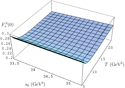
Figure 4: 3-dimensional plot of $F_{+}^{A}$.

From the above analysis, we get

$$F_{+}^{A}(q^{2}=0;T_{c})=0.256^{+0.0040}_{-0.0044}~{},$$ (34)

where the errors are from the variation of $s_{0}$ around $s_{b}$ by $\pm 1~{}{\rm GeV}^{2}$.

The observed axial kaons $K_{1}(1270)$ and $K_{1}(1400)$ are mixtures of ${}^{1}P_{1}$ and ${}^{3}P_{1}$ states. Their form factors are related via mixing angle $\theta$ as Cheng:2004yj ; PDG

$$F_{i}^{B\to K_{1}(1270)} = F_{i}^{A3}\sin\theta+F_{i}^{A}\cos\theta~{},$$ (35)

$$F_{i}^{B\to K_{1}(1400)} = F_{i}^{A3}\cos\theta-F_{i}^{A}\sin\theta~{}.$$

where $i=0,+,-$. Here, $F_{i}^{A3}$ are the ${}^{3}P_{1}$ form factors. We use the result of Cheng:2004yj , $F_{+}^{A3}(q^{2}=0)=0.11$. The mixing angle $\theta$ is not yet fixed precisely. Ref. Cheng:2004yj suggests $\theta=\pm 37^{\circ},~{}\pm 58^{\circ}$. Table 2 shows the values of $F_{+}^{B\to K_{1}(1270)}$ and $F_{+}^{B\to K_{1}(1400)}$ for these angles.

$\theta$	$37^{\circ}$	$-37^{\circ}$	$58^{\circ}$	$-58^{\circ}$
$F_{+}^{B\to K_{1}(1270)}$	$0.271$	$0.138$	$0.229$	$0.042$
$F_{+}^{B\to K_{1}(1400)}$	$-0.066$	$0.242$	$-0.159$	$0.276$

Table 2: $F_{+}^{B\to K_{1}(1270)}$ and $F_{+}^{B\to K_{1}(1400)}$ for various $\theta$.

For negative angles, we find

$$F_{+}^{B\to K_{1}(1270)}<F_{+}^{B\to K_{1}(1400)}~{}.$$ (36)

Since other parameters of the branching ratio are not so different in $B\to K_{1}(1270)\gamma$ and $B\to K_{1}(1400)\gamma$, one expects ${\cal B}(B\to K_{1}(1270)\gamma)<{\cal B}(B\to K_{1}(1400)\gamma)$ for the negative mixing angles. This is not consistent with the experimental data.

V Discussions and Conclusions

As discussed in jplee2 , the discrepancy between theory and experiment for ${\cal B}(B\to K_{1}(1270,~{}1400)\gamma$ is mainly due to the smallness of the relevant form factors. If there is no mixing (i.e., $\theta=0$), then $F_{+}^{B\to K_{1}(1270)}=F_{+}^{A}=0.256$. This is considerably larger than the previous LCSR result of Safir , $F_{+,{\rm Safir}}^{B\to K_{1}(1270)\gamma)}=0.14\pm 0.03$. The mixing effects are only $5.7\%$ and $-10.6\%$ for $\theta=37^{\circ},~{}58^{\circ}$, respectively. In Safir , only the asymptotic form of leading twist DA,

$$\phi^{\rm asy}_{\perp}(u)=6u(1-u)~{},$$ (37)

contributes to the sum rule. According to Eq. (31) of Safir ,

$$F_{+,{\rm Safir}}^{A}(0)=\frac{1}{2}e^{m_{B}^{2}/T}\left(\frac{m_{b}}{m_{B}^{2}f_{B}}\right)f_{A}^{\perp}m_{b}\int_{u_{0}}^{1}\frac{du}{u}\exp\left[-\frac{m_{b}^{2}+{\bar{u}}m_{A}^{2}}{uT}\right]\phi_{\perp}^{\rm asy}(u)~{}.\$$ (38)

It should be compared with Eq. (III). Eq. (III) improves Eq. (38) in three ways: (1) higher twist DAs are included; (2) non-asymptotic contributions are also included; (3) there is no term proportional to $m_{A}^{2}$ in $F_{+,{\rm Safir}}^{A}(0)$. With the parameter set used in the previous section, we have $F_{+,{\rm Safir}}^{A}(0;s=s_{b};T=T_{c})=0.187$. This is lager than the value of $F_{+,{\rm Safir}}^{B\to K_{1}(1270)\gamma)}=0.14\pm 0.03$. But if we take the sum rule window of Borel parameter adopted in Safir , $F_{+,{\rm Safir}}^{A}(0;s=s_{b};T=7.5~{}{\rm GeV}^{2})=0.151$, which assures the consistency of the present analysis. We can check how much the new improvements contribute to the form factor. The results are summarized in Table 3.

$F_{+,{\rm Safir}}^{A}(0)$	$~{}~{}~{}~{}~{}~{}~{}+$(3)	$~{}~{}~{}~{}~{}~{}~{}+$(3)$+$(2)	$~{}~{}~{}~{}~{}~{}~{}+$(3)$+$(2)$+$(1)
$0.187$	$~{}~{}~{}~{}~{}~{}~{}0.237$	$~{}~{}~{}~{}~{}~{}~{}0.155$	$~{}~{}~{}~{}~{}~{}~{}0.256$

Table 3: Contributions of new improvements. The parameter set used here is the same as that in the previous section. Conditions (1), (2), and (3) are explained in the text.

One finds that non-asymptotic and higher-twist DA contributions as well as non-zero mass effects are considerable.

The increase of the form factor will reduce the discrepancy between the theoretical predictions and experimental data jplee2 . At next-to-leading order of $\alpha_{s}$, the branching ratio of $B\to K_{1}\gamma$ is given by jplee1 ; jplee2

$${\cal B}(B^{0}\to K_{1}^{0}\gamma)=0.003\left(1-\frac{m_{K_{1}}^{2}}{m_{B}^{2}}\right)^{3}\Big{|}F_{+}^{A}(0)(-0.385-i0.014)+(f_{A}^{\perp}/{\rm GeV})(-0.024-i0.022)\Big{|}^{2}~{}.$$ (39)

The resulting branching ratios are given in Table 4.

$\theta$	$~{}~{}~{}~{}~{}~{}~{}0^{\circ}$	$~{}~{}~{}~{}~{}~{}~{}37^{\circ}$	$~{}~{}~{}~{}~{}~{}~{}58^{\circ}$	experiment Abe:2004kr
${\cal B}(B^{0}\to K_{1}(1270)^{0}\gamma)$	$~{}~{}~{}~{}~{}~{}~{}2.81$	$~{}~{}~{}~{}~{}~{}~{}3.14$	$~{}~{}~{}~{}~{}~{}~{}2.27$	$~{}~{}~{}~{}~{}~{}~{}4.28$
${\cal B}(B^{0}\to K_{1}(1400)^{0}\gamma)$	$~{}~{}~{}~{}~{}~{}~{}0.52$	$~{}~{}~{}~{}~{}~{}~{}0.14$	$~{}~{}~{}~{}~{}~{}~{}0.91$	$~{}~{}~{}~{}~{}~{}~{}<1.44$

Table 4: Branching ratios for various mixing angles in units of $10^{-5}$.

The enhancement is significant and the theoretical prediction becomes closer to the experimental data compared to the previous analysis jplee1 , though there is still a gap.

There are a few possibilities to improve further. Firstly, the precisions are different between Eqs. (39) and (III). Eq. (39) contains the hard spectator interactions which appear as a convolution between the jet function and the meson DAs. The DAs contributing to Eq. (39) are leading twist ones and of asymptotic form. It is thus necessary to include higher twist and non-asymptotic contributions in Eq. (39) at the same accuracy as was done in this work. Also, Eq. (III) contains terms proportional to $m_{A}^{2}$, but Eq. (39) is the result of heavy quark limit. One can easily expect that the next-to-leading order (NLO) of $\Lambda_{\rm QCD}/m_{b}$ corrections to the QCDF framework might include the terms of $m_{A}/m_{b}$, but there is no systematics so far. The hard spectator interactions are given by the convolution of hard kernel and meson DAs. Similar non-zero $m_{A}^{2}$ terms will also appear in the axial vector DAs to affect the hard spectator interactions. But this effect is not expected to be large. According to jplee1 , the hard spectator contributions amount to roughly about $~{}5\%$ at the amplitude level.

Secondly, $F_{+}^{A3}$ could be larger. Actually there is no clue about the size of $F_{+}^{A3}$, but it might be that $F_{+}^{A3}$ is comparable in size to $F_{+}^{A}$, just as in Cheng:2004yj . If this is the case, then the form factor can be enhanced via mixing

$$F_{+}^{B\to K_{1}(1270)}\approx 0.256\times(\sin\theta+\cos\theta)=0.35\sim 0.36~{},$$ (40)

for $\theta=37^{\circ},~{}58^{\circ}$, which results in a large branching ratio,

$${\cal B}(B^{0}\to K_{1}(1270)^{0}\gamma)\approx 5.3\times 10^{-5}~{}.$$ (41)

In conclusion, we have calculated $B\to K_{1B}$ form factor in LCSR. This analysis improves the previous one in a few respects by including higher twist DAs, non-asymptotic contributions, and non-zero $m_{A}^{2}$ terms. The value is rather larger than the previous calculation and that from the quark model result. Larger value is well accommodated to the experimental data. One needs more information about $K_{1A}$ and the mixing angle to reduce theoretical uncertainties. To go beyond the current work, one can include the NLO of $\alpha_{s}$ which might not be so different from that for $B\to K^{*}$ Ball:2004rg . And the study of $B\to K_{1}\gamma$ at higher accuracy comparable to this work will be necessary.

References

• (1) T. E. Coan et al. [CLEO Collaboration], Phys. Rev. Lett.  84, 5283 (2000) [arXiv:hep-ex/9912057]; S. Nishida et al. [Belle Collaboration], Phys. Rev. Lett.  89, 231801 (2002) [arXiv:hep-ex/0205025]; B. Aubert et al. [BABAR Collaboration], Phys. Rev. D 70, 091105 (2004) [arXiv:hep-ex/0409035].
• (2) K. Abe et al. [BELLE Collaboration], arXiv:hep-ex/0408138; H. Yang et al., Phys. Rev. Lett.  94, 111802 (2005) [arXiv:hep-ex/0412039].
• (3) M. Beneke, G. Buchalla, M. Neubert and C. T. Sachrajda, Nucl. Phys. B 591, 313 (2000) [arXiv:hep-ph/0006124].
• (4) M. Beneke and T. Feldmann, Nucl. Phys. B 592, 3 (2001) [arXiv:hep-ph/0008255].
• (5) M. Beneke, T. Feldmann and D. Seidel, Nucl. Phys. B 612, 25 (2001) [arXiv:hep-ph/0106067].
• (6) S. W. Bosch and G. Buchalla, Nucl. Phys. B 621, 459 (2002) [arXiv:hep-ph/0106081].
• (7) A. Ali and A. Y. Parkhomenko, Eur. Phys. J. C 23, 89 (2002) [arXiv:hep-ph/0105302].
• (8) J. P. Lee, Phys. Rev. D 69, 114007 (2004) [arXiv:hep-ph/0403034].
• (9) Y. J. Kwon and J. P. Lee, Phys. Rev. D 71, 014009 (2005) [arXiv:hep-ph/0409133].
• (10) M. Jamil Aslam and Riazuddin, Phys. Rev. D 72, 094019 (2005) [arXiv:hep-ph/0509082]; M. J. Aslam, [arXiv:hep-ph/0604025].
• (11) A. S. Safir, Eur. Phys. J. directC 3, 15 (2001) [arXiv:hep-ph/0109232].
• (12) P. Ball and R. Zwicky, Phys. Rev. D 71, 014029 (2005) [arXiv:hep-ph/0412079].
• (13) H. Y. Cheng and C. K. Chua, Phys. Rev. D 69, 094007 (2004) [arXiv:hep-ph/0401141].
• (14) K. C. Yang, JHEP 0510, 108 (2005) [arXiv:hep-ph/0509337].
• (15) G. Nardulli and T. N. Pham, Phys. Lett. B 623, 65 (2005) [arXiv:hep-ph/0505048].
• (16) D. Ebert, R. N. Faustov, V. O. Galkin and H. Toki, Phys. Rev. D 64, 054001 (2001) [arXiv:hep-ph/0104264].
• (17) P. Ball, V. M. Braun, Y. Koike and K. Tanaka, Nucl. Phys. B 529, 323 (1998) [arXiv:hep-ph/9802299].
• (18) P. Ball and V. M. Braun, Nucl. Phys. B 543, 201 (1999) [arXiv:hep-ph/9810475].
• (19) S. Eidelman et al. [Particle Data Group], Phys. Lett. B 592 (2004) 1.