In the Shadow of the Color Glass

Abstract

I give a brief overview of recent theoretical progress within perturbative QCD concerning the high–energy dynamics in the vicinity of the unitarity limit. Special attention is payed to the most recent developments concerning the relation between high–energy QCD and statistical physics, the role of the pomeron loops, and the transition from geometric scaling to diffusive scaling with increasing energy.

1 Motivation: The rise of the gluon distribution at HERA

The essential observation at the basis of the recent theoretical progress in the physics of hadronic interactions at high energy is the fact that high–energy QCD is the realm of high parton (gluon) densities and hence it can be studied from first principles, via weak coupling techniques. Anticipated by theoretical developments like the BFKL equation[1] and the GLR mechanism[2, 3] for gluon saturation, this observation has found its first major experimental foundation in the HERA data for electron–proton deep inelastic scattering (DIS) at small–$x$. As visible, e.g., on the H1 data shown in Fig. 1 (left figure), the gluon distribution $xG(x,Q^{2})$ rises very fast when decreasing Bjorken–$x$ at fixed $Q^{2}$ (roughly, as a power of $1/x$), and also when increasing $Q^{2}$ at a fixed value of $x$. The physical interpretation of such results is most transparent in the proton infinite momentum frame, where $xG(x,Q^{2})$ is simply the number of the gluons in the proton wavefunction which are localized within an area $\Delta x_{\perp}\sim 1/Q^{2}$ in the transverse plane and carry a fraction $x=k_{z}/P_{z}$ of the proton longitudinal momentum.

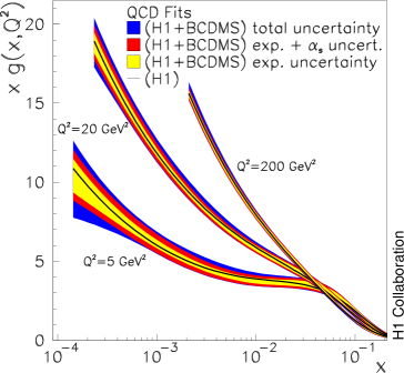
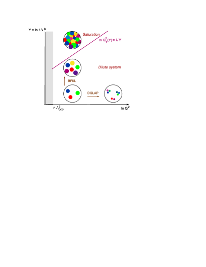
Figure 1: Left: Gluon distribution extracted at HERA (here, data from H1), as a function of $x$ in three bins of $Q^{2}$. Right: The ‘phase–diagram’ for QCD evolution suggested by the HERA data; each colored blob represents a parton with transverse area $\Delta x_{\perp}\sim 1/Q^{2}$ and longitudinal momentum $k_{z}=xP_{z}$.

Thus, without any theoretical prejudice, the HERA data suggest the physical picture illustrated in the right hand side of Fig. 1, which shows the distribution of partons in the transverse plane as a function of the kinematical variables for DIS in logarithmic units: $\ln Q^{2}$ and $Y\equiv\ln(1/x)$. The number of partons increases both with increasing $Q^{2}$ and with decreasing $x$, but whereas in the first case (increasing $Q^{2}$) the transverse area $\sim 1/Q^{2}$ occupied by every parton decreases very fast and more than compensates for the increase in their number — so, the proton is driven towards a regime which is more and more dilute —, in the second case (decreasing $x$) the partons produced by the evolution have roughly the same transverse area, hence their density is necessarily increasing.

Accordingly, the DGLAP equation[4] which describes the evolution with increasing $Q^{2}$ is naturally linear, and also local in $Q^{2}$. By contrast, the BFKL equation, which is the linear equation originally proposed[1] to describe the evolution with increasing energy, is non–local in transverse space and should be merely regarded as a linear approximation to more general evolution equations which are non–linear, i.e., which account for the interactions among the partons within the wavefunction. The non–linear effects are expected to become important in the region denoted as ‘saturation’ in Fig. 1, and also in the approach towards it when coming from the dilute region at large $Q^{2}$.

Mainly because of its complexity, the high–energy evolution in QCD is not as precisely known as the corresponding evolution with $Q^{2}$. Still, the intense theoretical efforts over the last years led to important conceptual clarifications and to new, more powerful, formalisms — among which, the effective theory for the Color Glass Condensate (CGC) [5, 6, 7] —, which encompass the non–linear dynamics in high–energy QCD to lowest order in $\alpha_{s}$ and allow for a unified picture of various high–energy phenomena ranging from DIS to heavy–ion, or proton–proton, collisions, and to cosmic rays.

These developments may explain some remarkable phenomena observed in the current experiments (like the ‘geometric scaling’ in the HERA data at small $x$[8, 9] and the particle production at forward rapidities in deuteron–gold collisions at RHIC[10]), and, moreover, they have potentially interesting predictions for the physics at LHC. It is my purpose in what follows to provide a brief, pedagogical, introduction to such new ideas, with emphasis on the physical picture and its consequences for deep inelastic scattering at high energy.

2 DIS: Dipole factorization & Saturation momentum

At small $x$, DIS is most conveniently computed by using the dipole factorization (see, e.g., Refs.[7] for more details and references). The small–$x$ quark to which couple the virtual photon is typically a ‘sea’ quark produced at the very end of a gluon cascade. It is then convenient to disentangle the electromagnetic process $\gamma^{*}q$, which involves this ‘last’ emitted quark, from the QCD evolution in the proton, which involves mostly gluons. This can be done via a Lorentz boost to the ‘dipole frame’ in which the struck quark appears as an excitation of the virtual photon, rather than of the proton. In this frame, the proton still carries most of the total energy, while the virtual photon has just enough energy to dissociate long before the scattering into a ‘color dipole’ (a $q\bar{q}$ pair in a color singlet state), which then scatters off the gluon fields in the proton. This leads to the following factorization:

$$\sigma_{\gamma^{*}p}(x,Q^{2})\,=\,\int_{0}^{1}{\rm d}z\int{\rm d}^{2}r\ |\Psi_{\gamma}(z,r;Q^{2})|^{2}\,\sigma_{\rm dipole}(x,r)$$ (1)

where $|\Psi_{\gamma}(z,r;Q^{2})|^{2}$ is the probability for the $\gamma^{*}\to q\bar{q}$ dissociation ($r$ is the dipole transverse size and $z$ the longitudinal fraction of the quark), and $\sigma_{\rm dipole}(x,r)$ is the total cross–section for dipole–proton scattering and represents the hadronic part of DIS. At high energy, the latter can be computed in the eikonal approximation as

$$\sigma_{\rm dipole}(x,r)\ =\ 2\int{\rm d}^{2}b\ \ T(r,b,Y)\,$$ (2)

where $T(r,b,Y)$ is the forward scattering amplitude for a dipole with size $r$ and impact parameter $b$. This is the quantity that we shall focus on. The unitarity of the $S$–matrix requires $T\leq 1$, with the upper limit $T=1$ corresponding to total absorbtion, or ‘black disk limit’.

But the unitarity constraint can be easily violated by an incomplete calculation, as we demonstrate now on the example of lowest–order (LO) perturbation theory. To that order, $T(r,b,Y)$ involves the exchange of two gluons between the dipole and the target. Each exchanged gluon brings a contribution $gt^{a}\bm{r}\cdot\bm{E}_{a}$, where $\bm{E}_{a}$ is the color electric field in the target. Thus, $T\sim g^{2}r^{2}\langle\bm{E}_{a}\cdot\bm{E}_{a}\rangle_{x}$, where the expectation value is recognized as the number of gluons per unit transverse area:

$$T(x,r,b)\,\sim\,\alpha_{s}\,r^{2}\,\frac{xG(x,1/r^{2})}{\pi R^{2}}\,\equiv\,\alpha_{s}\,n(x,Q^{2}\sim 1/r^{2})\,.$$ (3)

In the last equality we have identified the gluon occupation number : $n(x,Q^{2})=$ [number of gluons $xG(x,Q^{2})$] times [the area $1/Q^{2}$ occupied by each gluon] divided by [the proton transverse area $\pi R^{2}$].

Eq. (3) applies so long as $T\ll 1$ and shows that weak scattering (or ‘color transparency’) corresponds to low gluon occupancy $n\ll 1/\alpha_{s}$. But if naively extrapolated to very small values of $x$, this formula leads to unitarity violations : $T$ would eventually become larger than one ! Before this happens, however, new physical phenomena are expected to come into play and restore unitarity. As we shall see, these are non–linear phenomena, and are of two types: (i) multiple scattering, i.e., the exchange of more than two gluons between the dipole and the target, and (ii) gluon saturation, i.e., non–linear effects in the proton wavefunction which tame the rise of the gluon distribution at small $x$.

Eq. (3) also provides a criterion for the onset of unitarity corrections: These should become important when $T(x,r)\sim 1$ or $n(x,Q^{2})\sim 1/\alpha_{s}$. This condition can be solved for the saturation momentum, which is the value of the transverse momentum below which saturation effects are expected to be important in the gluon distribution. One thus finds

$$Q^{2}_{s}(x)\,\simeq\,{\alpha_{s}}\,\frac{xG(x,Q^{2}_{s})}{\,\pi R^{2}}\,\,\,\sim\,\,\frac{1}{x^{\lambda}}\,,$$ (4)

which grows with the energy as a power of $1/x$, since so does the gluon distribution before reaching saturation. In logarithmic units, the saturation line $\ln Q^{2}_{s}(Y)=\lambda Y$ is therefore a straight line, as illustrated in the right hand side of Fig. 1. This is the borderline between the dilute regime at high transverse momenta $k_{\perp}\gg Q_{s}(Y)$, where one expects the standard perturbation theory to apply, and a high–density region at low momenta $k_{\perp}\mathrel{\hbox to0.0pt{\raise 2.20013pt\hbox{$<$}\hss}{\lower 2.20013pt\hbox{$\sim$}}}Q_{s}(Y)$, where physics is non–linear. In fact, as we shall argue below, at high energy the effects of saturation can extend up to very high values of $k_{\perp}$, well above the saturation line.

3 BFKL evolution: The blowing–up gluon distribution

Within perturbative QCD, the emission of small–$x$ gluons is amplified by the infrared sensitivity of the bremsstrahlung process, whose iteration leads to the BFKL evolution (at least, for not too high energies). Fig. 2 shows the emission of a gluon which carries a fraction $x=k_{z}/p_{z}$ of the longitudinal momentum of its parent quark. When $x\ll 1$, the differential probability for this emission can be estimated as

$${\rm d}P_{\rm Brem}\,\simeq\,\frac{\alpha_{s}C_{F}}{2\pi^{2}}\,\frac{{\rm d}^{2}k_{\perp}}{k_{\perp}^{2}}\,\frac{{\rm d}x}{x}\,,$$ (5)

which is singular as $x\to 0$.

Figure 2: The lowest order diagram for bremsstrahlung.

Introducing the rapidity $Y\equiv\ln(1/x)$, and hence ${\rm d}Y={\rm d}x/x$, Eq. (5) shows that there is a probability of $\mathcal{O}{(\alpha_{s})}$ to emit one gluon per unit rapidity. The same would hold for the emission of a soft photon from an electron in QED. However, unlike the photon, the child gluon is itself charged with ‘colour’, so it can further emit an even softer gluon, with longitudinal fraction $x_{1}=q_{z}/k_{z}\ll 1$. When the rapidity is large, $\alpha_{s}Y\gg 1$, such successive emissions lead to the formation of gluon cascades, in which the gluons are ordered in rapidity and which dominate the small–$x$ part of the hadron wavefunction (see Fig. 3).

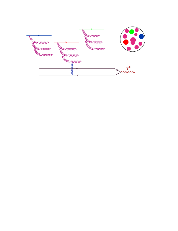
Figure 3: Gluon cascades produced by the high–energy (BFKL) evolution of the proton wavefunction, as probed by a small color dipole in DIS.

So long as the density is not too high, the gluons do not interact with each other and the evolution remains linear : when further increasing the rapidity in one more step ($Y\to Y+{\rm d}Y$), the gluons created in the previous steps incoherently act as color sources for the emission of a new gluon. This picture leads to the following, schematic, evolution equation

$$\frac{\partial n}{\partial Y}\,\simeq\,\omega\alpha_{s}n\qquad\Longrightarrow\quad n(Y)\,\propto\,{\rm e}^{\omega\alpha_{s}Y}\,,$$ (6)

which predicts the exponential rise of $n$ with $Y$. This is an oversimplified version of the BFKL (Balitsky-Fadin-Kuraev-Lipatov) equation[1] which captures the main feature of this evolution: the unstable growth of the gluon distribution. One knows by now that this growth is considerably tempered by NLO effects[11, 12], like the running of the QCD coupling or the requirement of energy conservation, but the basic fact that the gluon density increases exponentially with $Y$ is expected to remain true (independently of the order in $\alpha_{s}$) so long as one neglects the non–linear effects, or ‘gluon saturation’, in the evolution.

4 Non–linear evolution: JIMWLK equation and the CGC

Non–linear effects appear because gluons carry colour charge, so they can interact with each other (even when separated in rapidity) by exchanging gluons in the $t$–channel, as illustrated in Fig. 4. These interactions are amplified by the gluon density and thus they should become more and more important when increasing the energy.

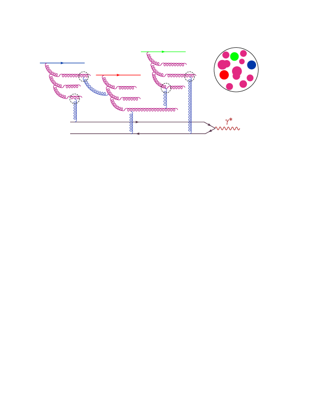
Figure 4: DIS in the presence of BFKL evolution, saturation and multiple scattering.

Back in 1983, L. Gribov, Levin and Ryskin[2] suggested that gluon saturation should proceed via $2\to 1$ ‘gluon recombination’, which is a process of order $\alpha_{s}^{2}n^{2}$ (cf. Fig. 4). To take this into account, they proposed the following, non–linear, generalization of Eq. (6) :

$$\frac{\partial n}{\partial Y}\,\simeq\,\alpha_{s}n\,-\,{\alpha_{s}^{2}}\,n^{2}\,=\,0\quad{\rm when}\quad n\,\,\sim\,\frac{1}{\alpha_{s}}\,\gg\,1$$ (7)

which has a fixed point $n_{\rm sat}=1/\alpha_{s}$ at high energy, as indicated above. That is, when $n$ is as high as $1/\alpha_{s}$, the emission processes (responsible for the BFKL growth) are precisely compensated by the recombination ones, and then the gluon occupation factor saturates at a fixed value.

Twenty years later, we know that the actual mechanism for gluon saturation in QCD is more subtle than just gluon recombination and that its mathematical description is considerably more involved than suggested by Eq. (7). This mechanism, as encoded in the effective theory for the CGC and its central equation, the JIMWLK equation (Jalilian-Marian, Iancu, McLerran, Weigert, Leonidov, and Kovner)[13, 6, 14], is the saturation of the gluon emission rate due to high density effects : At high density, the gluons are not independent color sources, rather they are strongly correlated with each other in such a way to ensure color neutrality[15, 16, 17] over a distance $\Delta x_{\perp}\sim 1/Q_{s}$. Accordingly, the soft gluons with $k_{\perp}\mathrel{\hbox to0.0pt{\raise 2.20013pt\hbox{$<$}\hss}{\lower 2.20013pt\hbox{$\sim$}}}Q_{s}$ are coherently emitted from a quasi–neutral gluon distribution, and then the emission rate ${\partial n}/{\partial Y}$ saturates at a constant value of $\mathcal{O}{(1)}$. Thus, in the regime that we call ‘saturation’, the gluon occupation factor keeps growing, but only linearly in $Y$ (i.e., as a logarithm of the energy)[18, 15]. Schematically:

$$\frac{\partial n}{\partial Y}\,=\,\chi(n)\,\approx\begin{cases}\displaystyle{\alpha_{s}n\,}&\text{ if\, $n\ll{1}/{\alpha_{s}}\ \ \Longrightarrow\ n\,\sim\,{\rm e}^{\alpha_{s}Y}\,,$}\\[9.95863pt] \displaystyle{\ 1}&\text{ if\, $n\mathrel{\hbox to0.0pt{\raise 2.20013pt\hbox{$>$}\hss}{\lower 2.20013pt\hbox{$\sim$}}}{1}/\alpha_{s}\ \ \ $}\displaystyle{\Longrightarrow\ n\,\sim\,Y-Y_{s}\,,}\end{cases}$$ (8)

where $\chi(n)$ is a non–linear function with the limiting behaviours displayed above and $Y_{s}(k_{\perp})$ is the saturation rapidity at which $n(Y_{s},k_{\perp})\sim 1/\alpha_{s}$.

The condition $Y>Y_{s}(k_{\perp})$ for given $k_{\perp}$ is tantamount to $k_{\perp}<Q_{s}(Y)$ for given $Y$, and the occupation number at saturation can be rewritten as

$$n(Y,k_{\perp})\,\sim\,Y-Y_{s}(k_{\perp})\,\sim\,\frac{1}{\alpha_{s}}\,\ln\frac{Q_{s}^{2}(Y)}{k_{\perp}^{2}}\qquad{\rm for}\qquad k_{\perp}<Q_{s}(Y)\,.$$ (9)

This shows that, due to saturation, the gluon spectrum at low $k_{\perp}$ rises only logarithmically with $1/k_{\perp}^{2}$, instead of the power–like divergence predicted by standard perturbation theory. (E.g., the bremsstrahlung spectrum (5) would diverge like $1/k_{\perp}^{2}$ if extrapolated towards $k_{\perp}\to 0$.) We see that $Q_{s}(Y)$ effectively acts as an ‘infrared cutoff’ in the calculation of the physical observables. This cutoff rises with the energy, cf. Eq. (4), and also with the atomic number $A$ in the case where the proton is replaced by a large nucleus[7]: $Q_{s}^{2}(Y,A)\sim{\rm e}^{\lambda Y}A^{1/3}$. Hence for sufficiently high energy and/or large values of $A$, $Q_{s}^{2}$ becomes much larger than $\Lambda_{\rm QCD}^{2}$ and then the weak–coupling description of the gluon distribution becomes indeed justified.

Eq. (8) is not yet the JIMWLK equation, but only a mean field approximation to it: In reality, one cannot write down a closed equation for the 2–point function $n(Y)=\langle\bm{E}_{a}\cdot\bm{E}_{a}\rangle_{Y}$, rather one has an infinite hierarchy for the $n$–point correlations $\langle A(1)A(2)\cdots A(n)\rangle_{Y}$ of the gluon fields. In the CGC formalism, these correlations are encoded into the weight function $W_{Y}[A]$ — a functional probability density for the field configurations:

$$\langle A(1)\,A(2)\,\cdots\,A(n)\rangle_{Y}\,=\,\int{\rm D}[A]\ W_{Y}[A]\ A(1)\,A(2)\,\cdots\,A(n)\,.$$ (10)

The average in Eq. (10) is similar to the ‘average over disorder’ that is usually performed in the study of amorphous materials, like glasses: the various target configurations scatter independently with the incoming projectile (indeed, their internal dynamics is ‘frozen’ over the characteristic time scale for scattering, by Lorentz time dilation), and the physical scattering amplitude is finally obtained by summing the contributions from all such configurations, with weight function $W_{Y}[A]$. This explains the concept of ‘glass’ in the ‘Color Glass Condensate’. The ‘color’ refers, of course, to the gluon color charge. Finally, the ‘condensate’ stays for the coherent state made by the gluons at saturation: this state has a large occupation number $n\sim 1/\alpha_{s}\gg 1$, as typical for a Bose condensate.

The JIMWLK equation[13, 6, 14] is a functional differential equation describing the evolution of $W_{Y}[A]$ with $Y$. Via Eq. (10), this functional equation generates an infinite hierarchy of ordinary evolution equations for the $n$–point functions of $A$, as anticipated.

5 DIS off the CGC: Unitarity & Geometric scaling

Let us now discuss the consequences of this non–linear evolution for the dipole scattering, and thus for DIS. The first observation is that, when the energy is so high that saturation effects become important on the dipole resolution scale (this requires $r\mathrel{\hbox to0.0pt{\raise 2.20013pt\hbox{$>$}\hss}{\lower 2.20013pt\hbox{$\sim$}}}1/Q_{s}(Y)$, cf. Eq. (3)), then multiple scattering becomes important as well: e.g., the double–scattering $T^{(2)}\sim(\alpha_{s}n)^{2}$ is of $\mathcal{O}{(1)}$, so like the single–scattering $T^{(1)}\sim\alpha_{s}n$. Thus, the behaviour of the scattering amplitude in the vicinity of the unitarity limit is the combined effect of BFKL growth, gluon saturation and multiple scattering.

Within the CGC formalism, multiple scattering is easily included in the eikonal approximation, thus yielding

$$\langle T(r,b)\rangle_{Y}\,=\,\int{\rm D}[A]\ \,W_{Y}[A]\,\,\,T(r,b)[A]\,,$$ (11)

where $T[A]$ is the amplitude corresponding to a given configuration of classical fields $A$, and is non–linear in the latter to all orders. By taking a derivative w.r.t. $Y$ and using the JIMWLK equation for $\partial W_{Y}/\partial Y$, one can deduce an evolution equation for the (average) dipole amplitude, with the following schematic structure (we ignore the transverse coordinates) :

$$\partial_{Y}\langle T\rangle\,=\,\alpha_{s}\langle T\rangle\,-\,\alpha_{s}\langle T^{2}\rangle\,.$$ (12)

Note that this is not a closed equation — the amplitude $\langle T\rangle$ for one dipole is related to the amplitude $\langle T^{2}\rangle$ for two dipoles — but only the first equation in an infinite hierarchy, originally obtained by Balitsky[19]. A closed equation can be obtained if one assumes factorization: $\langle T^{2}\rangle\approx\langle T\rangle\langle T\rangle$. This mean field approximation yields the Balitsky–Kovchegov (BK) equation[20], which applies when the target is sufficiently dense to start with (so like a large nucleus) and up to not too high energies (cf. Sec. 6).

Due to its simplicity, the BK equation has played an important role as a laboratory to study the effects of saturation and multiple scattering. As already manifest on its schematic form in Eq. (12), this equation has the fixed point $\langle T\rangle=1$ at high energy, i.e., it is consistent with unitarity and, moreover, it predicts that the black disk limit is eventually saturated: $\langle T(r)\rangle_{Y}=1$ when $r\mathrel{\hbox to0.0pt{\raise 2.20013pt\hbox{$>$}\hss}{\lower 2.20013pt\hbox{$\sim$}}}1/Q_{s}(Y)$. Hence, one can use this equation to determine the energy–dependence of the saturation momentum, that is, the slope $\lambda$ of the saturation line $\ln Q^{2}_{s}(Y)=\lambda Y$ (cf. Fig. 1). Remarkably, the growth of $\langle T\rangle_{Y}$ with $Y$ before reaching the saturation is entirely determined by the linearized version of the BK equation, i.e., the BFKL equation. This is important since, unlike the BK equation, the BFKL equation is presently known to NLO accuracy[11]. By using the latter (within the collinearly improved NLO–BFKL scheme of Refs.[21]), Triantafyllopoulos has computed[22] the saturation exponent $\lambda$ to NLO accuracy and thus found a value $\lambda\simeq 0.3$, which is roughly one third of the corresponding LO estimate[2].

Another crucial consequence of the non–linear evolution towards saturation — at least, at the level of the BK equation — is the property known as geometric scaling [8, 23] : Physics should be invariant along trajectories which run parallel to the saturation line because these are lines of constant gluon occupancy (see the l.h.s. of Fig. 5). In mathematical terms, this means that, up to relatively large momenta $Q^{2}\gg Q_{s}^{2}(Y)$, the observables should depend only upon the difference $\ln Q^{2}-\ln Q^{2}_{s}(Y)=\ln[Q^{2}/Q^{2}_{s}(Y)]$ from the saturation line, i.e., they should scale upon the ratio ${\tau}\equiv Q^{2}/Q^{2}_{s}(Y)$ rather than separately depend upon $Q^{2}$ and $Y$. In particular, the dipole scattering amplitude obeys $\langle T(r)\rangle_{Y}\approx\mathcal{T}(r^{2}Q^{2}_{s}(Y))$, which via the factorization formula (1) implies a similar scaling for the DIS cross–section (in the limit where the quark masses are negligible) : $\sigma_{\gamma^{*}p}(Y,Q^{2})\approx\sigma({\tau})$.

Remarkably, such a scaling has been identified in the HERA data, by Staśto, Golec-Biernat and Kwieciński[8] (see the r.h.s. plot in Fig. 5, which is taken from Ref.[8]), before its theoretical explanation has emerged[23, 24, 25] from studies of the BK equation. More recently, with the advent of more precise data for DIS diffraction at HERA, geometric scaling has been noticed in these data too[9].

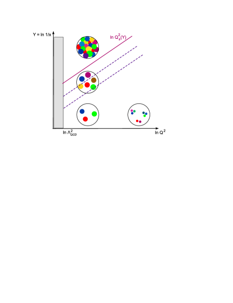
Figure 5: Left: Line of constant gluon occupancy at high $Q^{2}$. Right: Geometric scaling in the HERA data for $\sigma_{\gamma^{*}p}$ at $x\leq 0.01$; $\tau$ is the scaling variable, $\tau\equiv Q^{2}/Q^{2}_{s}(Y)$.

The outstanding feature of this scaling is the fact that this is a consequence of saturation which manifests itself up to relatively large transverse momenta, well above the saturation scale[23]. This is consistent with the HERA data, which show approximate scaling for all the experimental points at $x<0.01$, including values of $Q^{2}$ as high as 400 GeV². (For comparison, the saturation scale estimated from these data is $Q_{s}\simeq 1$ GeV for $x\sim 10^{-4}$.) It is also interesting to notice that the value for the saturation exponent coming out from such scaling fits to HERA is in agreement with its theoretical estimate[22] $\lambda\simeq 0.3$. Moreover, the violations of geometric scaling observed in the HERA data appear to be consistent[26] with theoretical expectations from the BFKL dynamics[23, 24].

The study of the BK equation has led to another surprise: Munier and Peschanski recognized[25] that this equation is in the same universality class as the FKPP equation which describes the mean field limit (corresponding to very large occupation numbers) of the classical stochastic process known as reaction–diffusion. This observation shed a new light on the physics of geometric scaling and, moreover, it helped clarifying the limitations of the mean field approximations and the essential role of fluctuations. In turn, this lead to substantial theoretical progress over the last two years that I shall briefly discuss in the next section.

6 Gluon number fluctuations and pomeron loops

Although the experimental results at HERA, and also at RHIC (see, e.g., the recent reviews in Ref.[28]), appear to be consistent with theoretical expectations based on the BK or JIMWLK equations, the latter are nevertheless incomplete (even to lowest order in $\alpha_{s}$) and thus cannot describe the actual dynamics in QCD at very high energies. Indeed, as recently recognized in Refs.[29, 30, 31, 32], these equations miss the effects of gluon–number fluctuations in the dilute regime, which however have a strong influence on the evolution with increasing energy, in particular, on the dynamics towards saturation. Such a strong sensitivity to fluctuations may look at a first sight surprising — the high–energy regime is characterized by high gluon occupancy, and therefore should be less affected by fluctuations —, but in fact this was already noticed in early studies of unitarization in the context of the dipole picture[33] and, more recently, it has been rediscovered within the context of the non–linear QCD evolution in the vicinity of the saturation line[29, 30]. This is also in agreement[31] with known properties of the reaction–diffusion process, as originally discovered in the context of statistical physics[27]. There are several ways to understand this sensitivity to fluctuations:

(i) First, one may recall from Fig. 4 that non–linear phenomena like gluon saturation and multiple scattering involve the simultaneous exchange of several gluons in the $t$–channel, and thus they probe correlations in the gluon distribution. At high energy, the most important such correlations are those generated via gluon splitting in the dilute regime: the ‘child’ gluons produced after a splitting are correlated with each other because they ‘remember’ about their common parent. These correlations manifest themselves in the difference $\langle nn\rangle-\langle n\rangle\langle n\rangle$ between the average pair density $\langle nn\rangle$ and its mean–field piece $\langle n\rangle\langle n\rangle$; thus, they describe gluon–number fluctuations[33, 29, 32]. Alternatively, these correlations are responsible for the difference $\langle T^{2}\rangle-\langle T\rangle\langle T\rangle$ (cf. Eq. (12)) and hence for violations of the factorization assumption underlying the BK equation[29, 30].

(ii) Second, one may notice that the driving force behind the high–energy evolution is the BFKL growth in the dilute tail of the gluon distribution at large transverse momenta $k_{\perp}\gg Q_{s}(Y)$. In that tail, the gluon occupation numbers are still low ($n\ll 1/\alpha_{s}$), so the fluctuations are relatively important, as demonstrated by intensive studies in the context of statistical physics (see Ref.[27] for a recent review and more references), which in turn have inspired similar studies within QCD[31, 34, 35].

Whereas the failure of the BK equation to accommodate these fluctuations was a priori clear, it somehow came as a surprise[32] that a similar failure holds also for the more general, Balitsky–JIMWLK, equations. The original confusion on this point came from the fact that these equations do generate correlations, as obvious from the fact that they correspond to non–trivial hierarchies. However, it turns out that the respective correlations represent color fluctuations alone, and thus disappear in the limit where the number of colors is large, $N_{c}\gg 1$, unlike the fluctuations in the particle number.

After this failure has been recognized[32], new equations have been proposed[32, 36, 37], which encompass both saturation and fluctuations in the limit where $N_{c}$ is large. These equations have been interpreted[38, 39, 40] as an effective theory for BFKL ‘pomerons’, in which the pomerons are allowed to dissociate and recombine with each other, like the molecules in the reaction–diffusion problem. Thus the perturbative solution to these equations involves pomeron loops. But the complexity of these ‘pomeron loop’ equations has so far hindered any systematic approach towards their solutions, including via numerical methods. The only properties of these solutions to be presently known come essentially from the correspondence with statistical physics[25, 30, 31, 32, 34, 35], which is however limited to asymptotically high energies and very small values of the coupling constant. The structure of these equations together with the known results about their solutions are discussed in more detail in other talks at this conference[43].

Figure 6: Dipole–hadron scattering in the fluctuation–dominated regime at very high energy. (a) a view along the collision axis; (b) a transverse view of the hadron, as ‘seen’ by a small dipole impinging at different impact parameters; (c) the simplified, black&white, picture of the hadron which is relevant for the average dipole amplitude.

Fig. 6 illustrates the most striking consequences of the evolution with pomeron loops, as probed in DIS at very high energy. The small blobs which are grey or black represent the regions of the target disk which are explored by the dipole with size $r$ at various impact parameters. The nuance of grey is representative of the intensity of the interaction, and thus of the local gluon density in the target (as viewed on the resolution scale $Q^{2}=1/r^{2}$ of the incoming dipole): a light grey spot denotes weak scattering ($T(r,b)\ll 1$), and hence a region with low gluon density, a white region means almost no gluons at all, and a black spot represents, of course, a region where the gluon density is so high that the black disk limit is reached: $T(r,b)\approx 1$. Thus, this picture suggests that, when probed on a fixed resolution scale $Q^{2}$, a hadron at very high energy may look extremely inhomogeneous. This lack of homogeneity has nothing to do with the initial conditions at low energy, rather it is the result of gluon–number fluctuations in the high–energy evolution. What is most remarkable about this picture is that, for sufficiently high energy, the average amplitude $\langle T(r)\rangle_{Y}$ (and thus the DIS cross–section) is completely dominated by the black spots up to very large values of $Q^{2}$, well above the average saturation momentum $\langle Q_{s}^{2}\rangle_{Y}$. That is, the average scattering may be weak, $\langle T(r)\rangle_{Y}\ll 1$, meaning that the target looks dilute on the average, yet this average is in fact controlled by rare fluctuations with unusually large density, for which $T\sim 1$. From the perspective of the incoming dipole, the hadron disk looks either black ($T\simeq 1$) or white ($T\simeq 0$), as illustrated in Fig. 6.c.

This physical picture has interesting consequences for the phenomenology. For instance, for DIS it predicts that, at sufficiently high energy, geometric scaling should be washed out by fluctuations[30] and replaced by a new type of scaling[31, 32], known as diffusive scaling[41] : instead of being a function of the ratio $Q^{2}/Q^{2}_{s}(Y)$, the DIS cross–section at high–energy should rather scale as a function of $Z\equiv\ln[Q^{2}/Q^{2}_{s}(Y)]/\sqrt{DY}$. (A similar scaling holds for the diffractive cross–section[41] in DIS and also for the cross–section for gluon production in proton–proton scattering at forward rapidity[42].) Here, $D$ is a ‘diffusion coefficient’ which measures the dispersion in the gluon distribution due to fluctuations. Its value is in principle determined by the pomeron loop equations, but it is presently unknown, because of the lack of a explicit solutions to the latter. Knowing the actual value of this parameter would be extremely important, since this would tell us at which energy we should expect diffusive scaling. (We expect[41] geometric scaling for $DY\ll 1$ and diffusive scaling for $DY\mathrel{\hbox to0.0pt{\raise 2.20013pt\hbox{$>$}\hss}{\lower 2.20013pt\hbox{$\sim$}}}1$.)

Figure 7: A ‘phase–diagram’ for the high–energy evolution with pomeron loops. Shown are the average saturation line and the scaling regions at $Q^{2}>\langle Q^{2}_{s}\rangle_{Y}$.

The previous discussion is summarized by the ‘phase–diagram’ in Fig. 7, which exhibits more structure than the original one in Fig. 1: In addition to the saturation line (to be now understood as the average saturation line $\ln\,\langle Q^{2}_{s}\rangle_{Y}\!=\lambda Y$ in the presence of fluctuations), this diagram also shows the kinematical domains for geometric scaling (at intermediate energies: $DY\ll 1$) and, respectively, diffusive scaling (at very high energy: $DY\mathrel{\hbox to0.0pt{\raise 2.20013pt\hbox{$>$}\hss}{\lower 2.20013pt\hbox{$\sim$}}}1$), which are seen to extend up to relatively large $Q^{2}\gg\langle Q^{2}_{s}\rangle_{Y}$. This is important as it shows that, for sufficiently high energies, the physics of saturation should manifest itself as the breakdown of the standard approximations at high $Q^{2}$ (like the leading–twist approximation or the collinear factorization) up to values of $Q^{2}$ which are so large that the average scattering amplitudes are truly small, far below the ‘black disk limit’.

The precise locations of the borderlines between these various regimes are not fully under control, because of the theoretical uncertainties on $\lambda$ and $D$. However, the experimental results at HERA and RHIC suggest that these experiments may have already probed the intermediate energy range characterized by geometric scaling (although in a kinematical domain which is only marginally perturbative). The experimental situation at the LHC will be even more favorable in that respect. The energies to be available there will be so high that the physics of saturation and the CGC could be explored within a wide kinematical range, including relatively large values of $Q^{2}$ for which the perturbation theory is fully reliable. In particular, there is the interesting possibility that the results at LHC will capture the transition from geometric to diffusive scaling (e.g., by varying the rapidity of the particles produced in $pp$ or $pA$ collisions[42]), and thus unveil the ultimate regime of QCD at ultrahigh energies.

References

- [1] L.N. Lipatov, Sov. J. Nucl. Phys. 23 (1976) 338; E.A. Kuraev, L.N. Lipatov and V.S. Fadin, Zh. Eksp. Teor. Fiz 72, 3 (1977); Ya.Ya. Balitsky, L.N. Lipatov, Sov. J. Nucl. Phys. 28 (1978) 822.
- [2] L.V. Gribov, E.M. Levin, and M.G. Ryskin, Phys. Rept. 100 (1983) 1.
- [3] A.H. Mueller and J. Qiu, Nucl. Phys. B268 (1986) 427.
- [4] V.N. Gribov and L.N. Lipatov, Sov. Journ. Nucl. Phys. 15 (1972), 438; G. Altarelli and G. Parisi, Nucl. Phys. B126 (1977), 298; Yu. L. Dokshitzer, Sov. Phys. JETP 46 (1977), 641.
- [5] L. McLerran and R. Venugopalan, Phys. Rev. D49 (1994) 2233; ibid. 49 (1994) 3352; ibid. 50 (1994) 2225.
- [6] E. Iancu, A. Leonidov and L. McLerran, Nucl. Phys. A692 (2001) 583; Phys. Lett. B510 (2001) 133; E. Ferreiro, E. Iancu, A. Leonidov and L. McLerran, Nucl. Phys. A703 (2002) 489.
- [7] E. Iancu, A. Leonidov and L. McLerran, hep-ph/0202270; E. Iancu and R. Venugopalan, hep-ph/0303204.
- [8] A.M. Stasto, K. Golec-Biernat and J. Kwiecinski, Phys. Rev. Lett. 86 (2001) 596.
- [9] C. Marquet and L. Schoeffel, hep-ph/0606079.
- [10] I. Arsene et al. [BRAHMS Collaboration], Phys. Rev. Lett. 93 (2004) 242303.
- [11] V.S. Fadin and L.N. Lipatov, Phys. Lett. B429 (1998) 127; G. Camici and M. Ciafaloni, Phys. Lett. B430 (1998) 349.
- [12] See the contributions by D. Colferai, S. Forte, K. Kutak in these proceedings.
- [13] J. Jalilian-Marian, A. Kovner, A. Leonidov and H. Weigert, Nucl. Phys. B504 (1997) 415; Phys. Rev. D59 (1999) 014014; J. Jalilian-Marian, A. Kovner and H. Weigert, Phys. Rev. D59 (1999) 014015; A. Kovner, J. G. Milhano and H. Weigert, Phys. Rev. D62 (2000) 114005.
- [14] H. Weigert, Nucl. Phys. A703 (2002) 823.
- [15] E. Iancu and L. McLerran, Phys. Lett. B510 (2001) 145.
- [16] A. H. Mueller, Nucl. Phys. B643 (2002) 501.
- [17] E. Iancu, K. Itakura, and L. McLerran, Nucl. Phys. A724 (2003) 181.
- [18] A. H. Mueller, Nucl. Phys. B558 (1999) 285.
- [19] I. Balitsky, Nucl. Phys. B463 (1996) 99; Phys. Lett. B518 (2001) 235.
- [20] Yu.V. Kovchegov, Phys. Rev. D60 (1999) 034008; ibid. D61 (1999) 074018.
- [21] G.P. Salam, JHEP 9807 (1998) 19; M. Ciafaloni, D. Colferai, Phys. Lett. B452 (1999) 372; M. Ciafaloni, D. Colferai, and G.P. Salam, Phys. Rev. D60 (1999) 114036.
- [22] D.N. Triantafyllopoulos, Nucl. Phys. B648 (2003) 293.
- [23] E. Iancu, K. Itakura, and L. McLerran, Nucl. Phys. A708 (2002) 327.
- [24] A.H. Mueller and D.N. Triantafyllopoulos, Nucl. Phys. B640 (2002) 331.
- [25] S. Munier and R. Peschanski, Phys. Rev. Lett. 91 (2003) 232001.
- [26] E. Iancu, K. Itakura and S. Munier, Phys. Lett. B590 (2004) 199.
- [27] For a recent review, see W. Van Saarloos, Phys. Rep. 386 (2003) 29.
- [28] M. Gyulassy, L. McLerran, Nucl. Phys. A750 (2005) 30; J.-P. Blaizot, F. Gelis, ibid. 148.
- [29] E. Iancu and A.H. Mueller, Nucl. Phys. A730 (2004) 494.
- [30] A.H. Mueller and A.I. Shoshi, Nucl. Phys. B692 (2004) 175.
- [31] E. Iancu, A.H. Mueller and S. Munier, Phys. Lett. B606 (2005) 342.
- [32] E. Iancu and D.N. Triantafyllopoulos, Nucl. Phys. A756 (2005) 419.
- [33] A.H. Mueller, Nucl. Phys. B415 (1994) 373; ibid. B437 (1995) 107; A.H. Mueller and G.P. Salam, ibid. B475 (1996) 293.
- [34] G. Soyez, Phys. Rev. D72 (2005) 016007.
- [35] R. Enberg, K. Golec–Biernat, and S. Munier, Phys. Rev. D72 (2005) 074021.
- [36] A.H. Mueller, A.I. Shoshi, S.M.H. Wong, Nucl. Phys. B715 (2005) 440.
- [37] E. Iancu and D.N. Triantafyllopoulos, Phys. Lett. B610 (2005) 253.
- [38] E. Levin and M. Lublinsky, Nucl. Phys. A763 (2005) 172.
- [39] J.-P. Blaizot et al, Phys. Lett. B615 (2005) 221.
- [40] E. Iancu, G. Soyez, D.N. Triantafyllopoulos, Nucl. Phys. A768 (2006) 194.
- [41] Y. Hatta et al, Nucl. Phys. A773 (2006) 95.
- [42] E. Iancu, C. Marquet, and G. Soyez, arXiv:hep-ph/0605174.
- [43] See the contributions by Y. Hatta, C. Marquet, G. Soyez in these proceedings.