SLAC–PUB–12034 hep-ph/0608027

Bootstrapping One-Loop QCD Amplitudes  

Carola F. Berger

Stanford Linear Accelerator Center
Stanford University, Stanford, California 94309 USA

ABSTRACT

We review the recently developed bootstrap method for the computation of high-multiplicity QCD amplitudes at one loop. We illustrate the general algorithm step by step with a six-point example. The method combines (generalized) unitarity with on-shell recursion relations to determine the not cut-constructible, rational terms of these amplitudes. Our bootstrap approach works for arbitrary configurations of gluon helicities and arbitrary numbers of external legs.

1 Introduction

The Large Hadron Collider (LHC), which is scheduled to begin operation in 2007, will provide new insight into the main missing piece of the Standard Model, the origin of electroweak symmetry breaking, and potentially discover new physics beyond the Standard Model. Discoveries at the LHC require a thorough understanding of Standard Model processes, all of which have many particles in the final state. Similarly, very precise knowledge of backgrounds and expected signals at the future International Linear Collider is required. In order to fully exploit the potential of both machines, many high-multiplicity processes need to be computed to as high accuracy as possible, which entails the computation of multi-leg amplitudes to at least one-loop order. This is a challenging endeavor, and traditional methods based on the direct analytical evaluation of an enormous magnitude of Feynman diagrams are not optimized for this task.

Here we review a recently developed method that combines on-shell recursion relations with (generalized) unitarity to compute one-loop multi-gluon amplitudes recursively, thereby “recycling” information from amplitudes with fewer legs [1, 2, 3]. The bootstrap method works for arbitrary helicity configurations. Moreover, in some cases, the recursion can be solved explicitly, yielding all-multiplicity expressions for one-loop gluon amplitudes [1, 2, 3, 4, 5]. Our bootstrap method relies only on factorization properties of the amplitudes as well as unitarity, and should therefore be amenable to an extension to amplitudes with external fermions and massive partons.

After a brief summary of our notation, we review the on-shell recursion relations for tree-level amplitudes derived via Cauchy’s theorem by continuing the physical amplitudes into the complex plane. At one loop, several new features arise, and Cauchy’s theorem is not immediately applicable. We show how to overcome these difficulties with the bootstrap approach, which combines the information from unitarity and two continuations in independent complex parameters. We summarize our results and some open problems and give an outlook on possible future directions and applications of the method.

2 Notation

In the following, we use the spinor helicity formalism (see for example [6] and references therein) to express the amplitudes in terms of spinor inner products,

$$\left\langle j\,l\right\rangle=\langle j^{-}|l^{+}\rangle=\bar{u}_{-}(k_{j})u_{+}(k_{l})\,,\hskip 56.9055pt\left[j\,l\right]=\langle j^{+}|l^{-}\rangle=\bar{u}_{+}(k_{j})u_{-}(k_{l})\,,$$ (1)

where $u_{\pm}(k)$ is a massless Weyl spinor with momentum $k$ and positive or negative chirality, respectively, which we also write as,

$$\lambda_{i}\equiv u_{+}(k_{i}),\qquad{\tilde{\lambda}}_{i}\equiv u_{-}(k_{i})\,.$$ (2)

Furthermore, we strip off all color information, as well as coupling constants, and compute only the leading-color amplitudes. We employ the following supersymmetric decomposition of the leading-color one-loop QCD amplitudes in the four-dimensional helicity scheme [7],

$$A_{n;1}^{\rm QCD} = A^{{\cal N}=4}_{n;1}-4A^{{\cal N}=1}_{n;1}+A^{{\cal N}=0}_{n;1}+{n_{\mskip-2.0muf}\over N_{c}}\Bigl{(}A^{{\cal N}=1}_{n;1}-A^{{\cal N}=0}_{n;1}\Bigr{)}\,,$$ (3)

where $n_{\mskip-2.0muf}$ is the number of active quark flavors in QCD. The contributions from the ${\cal N}=4$ and ${\cal N}=1$ supersymmetric multiplets are completely cut-constructible, that is, they contain only (poly)logarithms and associated constants ($\pi^{2}$) and are thus computable via (generalized) unitarity. The remaining non-supersymmetric ${\cal N}=0$ contribution from a scalar running in the loop has both cut-constructible and rational parts. It is the latter part that we will compute via on-shell recursion relations. In the following we will suppress the ${\cal N}=0$ superscript and write $A_{n}\equiv A^{{\cal N}=0}_{n;1}$.

For further information and our notational conventions we refer to [2] and the lecture notes [6].

3 On-Shell Recursion Relations at Tree Level

3.1 Review of the Proof at Tree Level

Here we briefly review the on-shell recursion relations found in ref. [8] and proven in ref. [9] for tree level amplitudes. For further details we refer to these papers.

At tree level, the on-shell recursion relations rely on general properties of complex functions as well as factorization properties of scattering amplitudes. The proof [9] of the tree-level relations employs a parameter-dependent “$[j,l\rangle$” shift of two of the external massless spinors, $j$ and $l$, in an $n$-point process,

$${[j,l\rangle}:\hskip 56.9055pt{\tilde{\lambda}}_{j}\rightarrow{\tilde{\lambda}}_{j}-z{\tilde{\lambda}}_{l}\,,\hskip 56.9055pt\lambda_{l}\rightarrow\lambda_{l}+z\lambda_{j}\,.$$ (4)

where $z$ is a complex number. The corresponding momenta are then continued in the complex plane as well so that they remain massless, $k_{j}^{2}(z)=0=k_{l}^{2}(z)$, and overall momentum conservation is maintained.

An on-shell amplitude containing the momenta $k_{j}$ and $k_{l}$ then also becomes parameter-dependent,

$$A(z)=A(k_{1},\ldots,k_{j}(z),k_{j+1},\ldots,k_{l}(z),\ldots,k_{n}).$$ (5)

When $A$ is a tree amplitude or finite one-loop amplitude, $A(z)$ is a rational function of $z$. The physical amplitude is given by $A(0)$.

We can then use Cauchy’s theorem,

$${1\over 2\pi i}\oint_{C}{dz\over z}\,A(z)=0\,,$$ (6)

where the contour $C$ is taken around the circle at infinity, and the integral vanishes if the complex continued amplitude $A(z)$ vanishes as $z\rightarrow\infty$. Evaluating the integral as a sum of residues, we can then solve for the physical amplitude $A(0)$ to obtain,

$$A(0)=-\sum_{{\rm poles}\ \alpha}\mathop{\rm Res}_{z=z_{\alpha}}{A(z)\over z}\,.$$ (7)

Figure 1: Schematic representation of a typical tree recursive contribution to eq. (10). The labels ‘$T$’ refer to on-shell tree amplitudes. The momenta $\hat{j}$ and $\hat{l}$ are complex continued, on-shell momenta.

As explained in ref. [9], at tree level $A(z)$ only has simple poles, as schematically illustrated in fig. 2 (a). These poles arise when shifting the propagators in the amplitude. For example,

$$\frac{i}{K_{r\dots l\dots s}^{2}}\rightarrow\frac{i}{K_{r\dots s}^{2}+z\left\langle\smash{j}{\vphantom{1}}^{-}\right|{{\raise 0.91666pt\hbox to9.20833pt{\hss/\hss}\hbox to0.0pt{\hss$K$}}_{r\ldots s}}\left|\smash{l}{\vphantom{1}}^{-}\right\rangle}\,,$$ (8)

if the set of legs $\{r,\dots,s\}$ contains leg $l$, which is shifted according to eq. (4). The complex continued amplitude is then schematically given by,

$$A\rightarrow A(z)=\sum_{r,s}\sum_{h}A^{h}_{L}(z){i\over K_{r\dots s}^{2}+z\left\langle\smash{j}{\vphantom{1}}^{-}\right|{{\raise 0.91666pt\hbox to9.20833pt{\hss/\hss}\hbox to0.0pt{\hss$K$}}_{r\ldots s}}\left|\smash{l}{\vphantom{1}}^{-}\right\rangle}A^{-h}_{R}(z)\,,$$ (9)

where $h=\pm 1$ labels the helicity of the intermediate state, and the labels $L$ and $R$ denote amplitudes with fewer legs, which the propagator eq. (8) connects. There is generically a double sum, labelled by $r,s$, dividing the set of legs into partitions with legs $j$ and $l$ always appearing on opposite sides of the $z$-dependent propagator. Therefore, each residue in eq. (7) is given by factorizing the shifted amplitude on the poles in momentum invariants, so that at tree level,

$$A(0)=\sum_{r,s}\sum_{h}A^{h}_{L}(z=z_{rs}){i\over K_{r\cdots s}^{2}}A^{-h}_{R}(z=z_{rs})\,.$$ (10)

The squared momentum associated with that pole, $K_{r\cdots s}^{2}$, is evaluated in the unshifted kinematics; whereas the on-shell amplitudes with fewer legs, $A_{L}$ and $A_{R}$, are evaluated in kinematics that have been shifted by eq. (4) with $z=z_{rs}$, where eq. (8) has a pole,

$$z_{rs}=-{K_{r\cdots s}^{2}\over\left\langle\smash{j}{\vphantom{1}}^{-}\right|{{\raise 0.91666pt\hbox to9.20833pt{\hss/\hss}\hbox to0.0pt{\hss$K$}}_{r\ldots s}}\left|\smash{l}{\vphantom{1}}^{-}\right\rangle}\,.$$ (11)

In the following, such shifted, on-shell momenta will be denoted by $k(z=z_{rs})\equiv\hat{k}$. A typical contribution to the sums in eq. (10) is illustrated in fig. 1.

We have thus succeeded in expressing the $n$-point amplitude $A$ in terms of sums over on-shell, but complex continued, amplitudes with fewer legs, which are connected by scalar propagators. For certain helicity configurations, this recursion relation can be solved explicitly, leading to new all-multiplicity expressions for these amplitudes.

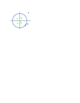
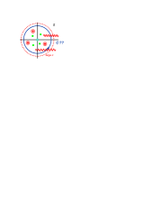
                           (a)                                           (b)

Figure 2: Illustration of the pole-structure in the complex plane for QCD amplitudes at (a) tree level, and (b) at the one-loop level. The point at the origin symbolizes the physical amplitude at $z=0$. Branch cuts are drawn as zigzagged lines. Simple poles are depicted as green dots, non-standard poles as red circled dots. The dashed line symbolizes the large-parameter contribution.

3.2 New Features at the One-Loop Level

The proof reviewed above relies on two properties of the complex continued tree level amplitude:

• The amplitude only has simple poles, which correspond to physical multiparticle and collinear factorizations.

• The amplitude vanishes at infinity.

These properties do not depend on the specific details of the gauge theory under consideration. Therefore, at tree level, the application of the recursion relation eq. (10) has been extended beyond multi-gluon amplitudes, to the computation of amplitudes including fermions, scalars, and massive partons, to the computation of gravity amplitudes, and of Higgs amplitudes produced via a heavy quark loop, in the effective theory where the heavy quark has been integrated out. Further details and references can be found in refs. [5, 10].

At loop level, however, these properties do not hold in general, and several new features arise:

• The (poly)logarithmic terms of the amplitude have spurious, unphysical, singularities, which however cancel in the full amplitude against corresponding terms in the rational part. These spurious singularities are already present in real kinematics. For example, terms of the following form arise,

  $${\ln(r)\over(1-r)^{2}}\,,$$ (12)

  which is singular as $r\rightarrow 1$. Such spurious singularities complicate the application of Cauchy’s theorem because it requires to sum over all poles, whether physical or unphysical.

• The amplitude develops branch cuts in the complex plane that stem from the complex continuation of (poly)logarithms.

• The complex continued amplitude contains double poles $\sim\frac{\left\langle a\,b\right\rangle}{{\left[a\,b\right]}^{2}}$, and ‘unreal’ poles $\sim\frac{\left\langle a\,b\right\rangle}{{\left[a\,b\right]}}$. In real kinematics, expressions of this form have only a single pole, or are not singular, respectively, because the spinor products $\left\langle a\,b\right\rangle$ and $\left[a\,b\right]$ differ only by a phase. With the complex continuation eq. (4) these ratios of spinor products develop (double) poles. Such poles arise in two-particle channels with like helicities, and the complex factorization properties in these channels are not yet fully understood. We term these channels ‘non-standard’.

• The amplitude does not vanish as $z\rightarrow\infty$.

These new features are illustrated in fig. 2 (b). For general helicity configurations, as explained in ref. [2], one can choose a pair of shifted momenta that avoids either non-standard channels or large-parameter contributions, but in general not both.

4 The Bootstrap Method

The bootstrap method developed in refs. [1, 2] systematically deals with the aforementioned complications. We use the term ‘bootstrap’ because we “assume that very general consistency criteria are sufficient to determine the whole theory completely” [11]. In the present case, the consistency criteria we employ are unitarity, to determine the branch cuts, and factorization, to obtain the rational remainder via on-shell recursion relations. The self-consistency of the approach and thus the correctness of the results is checked via collinear and multiparticle factorization limits in all possible channels. Any omitted terms would spoil the correct factorization behavior.

4.1 Branch Cuts from Unitarity

In order to deal with branch cuts and associated spurious singularities, we begin by decomposing the amplitude into ‘pure-cut’ and ‘rational’ parts,

$$A_{n}(z)=c_{\Gamma}\Bigl{[}C_{n}(z)+R_{n}(z)\Bigr{]}\,,$$ (13)

where we have explicitly taken an ubiquitous one-loop factor $c_{\Gamma}$ outside of $C_{n}(z)$ and $R_{n}(z)$,

$$c_{\Gamma}={1\over(4\pi)^{2-\epsilon}}{\Gamma(1+\epsilon)\Gamma^{2}(1-\epsilon)\over\Gamma(1-2\epsilon)}\,.$$ (14)

The rational parts are defined by setting all logarithms, polylogarithms, and associated $\pi^{2}$ terms to zero,

$$R_{n}(z)\equiv{1\over c_{\Gamma}}A_{n}(z)\Bigr{|}_{\rm rat}={1\over c_{\Gamma}}A_{n}(z)\biggr{|}_{\ln,\mathop{\rm Li}\nolimits,\pi^{2}\rightarrow 0}\,.$$ (15)

The pure-cut terms are the remaining terms, all of which must contain logarithms, polylogarithms, or $\pi^{2}$ terms. In the following we assume that the cut containing terms have been computed via (generalized) unitarity or other means (see, e. g. [12, 13, 14] and references therein), and derive an on-shell recursion for the rational remainder.

As mentioned above, the presence of spurious, unphysical singularities in the pure-cut parts complicates this task. These spurious poles cancel in the full amplitude. We will therefore ‘complete the cut’ by adding rational terms ${\widehat{CR}}$ to the pure-cut parts that eliminate these spurious poles from the beginning. For example, we add a term proportional to $\sim\frac{1}{1-r}$ to eq. (12) to eliminate the singularity as $r\rightarrow 1$. Effectively, we replace certain combinations of (poly)logarithms by $\mathop{\rm L{}}\nolimits_{i}$- and $\mathop{\rm Ls}\nolimits_{i}$-functions (see e. g. ref. [3] for definitions). For example, we replace eq. (12) with

$$\mathop{\rm L{}}\nolimits_{1}(r)={\frac{\ln(r)}{(1-r)}+1\over 1-r}\,.$$ (16)

Instead of the decomposition eq. (13) we now have,

$$A_{n}(z)=c_{\Gamma}\Bigl{[}\bigg{(}C_{n}(z)+{\widehat{CR}}_{n}(z)\bigg{)}+\bigg{(}R_{n}(z)-{\widehat{CR}}_{n}(z)\bigg{)}\Bigr{]}\equiv c_{\Gamma}\Bigl{[}{\widehat{C}}_{n}(z)+{\widehat{R}}_{n}(z)\Bigr{]}\,,$$ (17)

where we have defined ${\widehat{C}}\equiv C+{\widehat{CR}}$ and ${\widehat{R}}=R-{\widehat{CR}}$. Of course, such a cut-completion is not unique. Also, when constructing a recursion relation for the rational remainder, we need to take into account that ${\widehat{C}}_{n}$ already contains rational terms from this cut-completion in order to avoid double counting. The resulting full amplitude is then unambiguous.

4.2 On-Shell Recursion for Rational Terms

Since cut and rational parts factorize separately [1], we can now apply Cauchy’s theorem to eq. (17). Note that ${\widehat{C}}_{n}(z)$ may have (spurious) contributions as $z\rightarrow\infty$, denoted by $\mathop{\rm Inf}{\widehat{C}}_{n}$, which we can subtract off, since we know ${\widehat{C}}_{n}(0)$ (and thus ${\widehat{C}}_{n}(z)$). We obtain,

$$A_{n}(0)=\mathop{\rm Inf}A_{n}+c_{\Gamma}\Biggl{[}{\widehat{C}}_{n}(0)-\mathop{\rm Inf}{\widehat{C}}_{n}-\sum_{{\rm poles}\ \alpha}\mathop{\rm Res}_{z=z_{\alpha}}{R_{n}(z)\over z}+\sum_{{\rm poles}\ \alpha}\mathop{\rm Res}_{z=z_{\alpha}}{{\widehat{CR}}_{n}(z)\over z}\Biggr{]}\,.$$ (18)

Here, we have taken into account the fact that the full amplitude does not necessarily vanish at infinity under the chosen shift. This contribution is denoted by $\mathop{\rm Inf}A_{n}$. Its formal operator definition is the extraction of the constant $z^{0}$ term in a Laurent expansion of $A_{n}(z)$ around $z=\infty$,

$$\mathop{\rm Inf}A_{n}(z)=\mathop{\rm Inf}\,\left[\sum_{i}\left(a^{(i)}z^{i}+\frac{b^{(i)}+\ln(1/z)c^{(i)}+\ln^{2}(1/z)d^{(i)}}{z^{i}}\right)\right]=a^{(0)}\,.$$ (19)

The subtraction of $\mathop{\rm Inf}{\widehat{C}}_{n}$ is necessary, because we essentially perform a contour integral over the function $\left[A_{n}-\mathop{\rm Inf}A_{n}\right]-{\widehat{C}}_{n}$, which should vanish such that we are able to close the contour at infinity. If $\mathop{\rm Inf}{\widehat{C}}$ does not vanish, we need to subtract it off, such that the contour integral over $\left[A_{n}-\mathop{\rm Inf}A_{n}\right]-\big{[}{\widehat{C}}_{n}-\mathop{\rm Inf}{\widehat{C}}_{n}\big{]}$ vanishes, and Cauchy’s theorem can be applied.

Double counting between the rational terms in the cut completion ${\widehat{C}}_{n}$ and the rational remainder is avoided by the ‘overlap terms’ $O_{n}$,

$$O_{n}\equiv\sum_{{\rm poles}\ \alpha}\mathop{\rm Res}_{z=z_{\alpha}}{{\widehat{CR}}_{n}(z)\over z}\,,$$ (20)

where in general every channel that gets shifted according to eq. (4) contributes to the sum, as illustrated in fig. 3, but for specific cut completions, individual channels may vanish. $O_{n}$ can be computed straightforwardly from the cut completion.

Figure 3: Diagrammatic representation of overlap contributions. Each overlap diagram corresponds to a physical channel.

Finally, the sum over residues of the rational part again results in a recursion relation, quite analogous to the tree-level case,

$$-\sum_{{\rm poles}\ \alpha}\mathop{\rm Res}_{z=z_{\alpha}}{R_{n}(z)\over z} \equiv R^{D}_{n}(k_{1},\ldots,k_{n})$$ (21)

$$= \hskip-2.84544pt\sum_{r,s}\,\sum_{h}\Biggl{\{}A^{{\rm tree}\,,h}_{L}(z=z_{rs}){i\over K_{r\ldots s}^{2}}R_{R}^{-h}(z=z_{rs})$$

$$\qquad\quad+\,R_{L}^{h}(z=z_{rs}){i\over K_{r\ldots s}^{2}}A^{{\rm tree}\,,-h}_{R}(z=z_{rs})$$

$$\qquad\quad+\,A^{{\rm tree}\,,h}_{L}(z=z_{rs}){i{\cal F}(K_{r\ldots s}^{2})\over K_{r\ldots s}^{2}}A^{{\rm tree}\,,-h}_{R}(z=z_{rs})\Biggr{\}}\,.$$

In the first two terms the scalar propagator connects the rational part of an on-shell loop amplitude with an on-shell tree amplitude, the last term corresponds to a one-loop correction to the propagator [15]. Eq. (21) is schematically illustrated in fig. 4. However, for a given shift, we may encounter non-standard channels with as yet unknown factorization behavior, which arise from two-particle channels with like-helicity gluons,

$$R^{D}_{n}\equiv R^{D,{\rm\,recursive}}_{n}+R^{D,{\rm\,non-standard}}_{n}\,,$$ (22)

where $R^{D,{\rm\,non-standard}}$ involves $R_{3}(k_{i}^{\pm},k_{i+1}^{\pm},-\hat{K}_{i\,(i+1)})$ channels ($i$ or $i+1=\hat{j}$ or $\hat{l}$ for a ${[j,l\rangle}$-shift).

Figure 4: Schematic representation of one-loop recursive contributions to eq. (21). The labels ‘$T$’ and ‘$L$’ refer to tree and loop vertices.

In summary, after attempting to construct a recursion relation for the rational terms, we have,

$$A_{n}(0)={\color[rgb]{1,0,0}\mathop{\rm Inf}A_{n}}+c_{\Gamma}\Biggl{[}{\widehat{C}}_{n}(0)-\mathop{\rm Inf}{\widehat{C}}_{n}+R^{D,{\rm\,recursive}}_{n}+{\color[rgb]{1,0,0}R^{D,{\rm\,non-standard}}_{n}}+O_{n}\Biggr{]}\,,$$ (23)

which has two unknown contributions, the large-parameter contribution $\mathop{\rm Inf}A$, and the contribution from channels with not yet fully understood factorization behavior, $R^{D,{\rm\,non-standard}}$.

4.3 Pairs of Shifts to the Rescue

As shown in [2] by empirical study of known amplitudes, in general we can find shifts (4) which are either free of large-parameter contributions or free of contributions from non-standard channels, but not both. However, by using a pair of shifts in two independent complex parameters, we can construct a recursion relation which determines all unknown terms in eq. (23).

We use the primary shift eq. (4), and an auxiliary shift of two different legs,

$${[a,b\rangle}:\hskip 56.9055pt{\tilde{\lambda}}_{a}\rightarrow{\tilde{\lambda}}_{a}-w{\tilde{\lambda}}_{b}\,,\hskip 56.9055pt\lambda_{b}\rightarrow\lambda_{b}+w\lambda_{a}\,.$$ (24)

We obtain the following recursion relations for the amplitude,

$$A_{n}(0) = {\color[rgb]{1,0,0}\mathop{\rm Inf}\limits_{{[j,l\rangle}}{A_{n}}}+c_{\Gamma}\Biggl{[}{\widehat{C}}_{n}(0)-\mathop{\rm Inf}\limits_{{[j,l\rangle}}{{\widehat{C}}_{n}}+R^{D,{\rm\,recursive}\,{[j,l\rangle}}_{n}+O_{n}^{{[j,l\rangle}}\Biggr{]}\,,$$ (25)

$$A_{n}(0) = c_{\Gamma}\Bigl{[}{\widehat{C}}_{n}(0)-\mathop{\rm Inf}\limits_{{[a,b\rangle}}{{\widehat{C}}_{n}}+R^{D,{\rm\,recursive}\,{[a,b\rangle}}_{n}+{\color[rgb]{1,0,0}R^{D,{\rm\,non-standard}\,{[a,b\rangle}}_{n}}+O_{n}^{{[a,b\rangle}}\Bigr{]}\,,$$ (26)

where we have indicated with additional superscripts which shift has been employed. Applying the primary shift eq. (4) to the auxiliary recursion (26), we can extract the large-parameter behavior of the primary shift according to eq. (19),

$${\color[rgb]{1,0,0}\mathop{\rm Inf}\limits_{{[j,l\rangle}}{A_{n}}}=c_{\Gamma}\Bigl{[}\mathop{\rm Inf}\limits_{{[j,l\rangle}}{{\widehat{C}}_{n}}-\mathop{\rm Inf}\limits_{{[j,l\rangle}}{\bigg{(}\mathop{\rm Inf}\limits_{{[a,b\rangle}}{{\widehat{C}}_{n}}\bigg{)}}+\mathop{\rm Inf}\limits_{{[j,l\rangle}}{R^{D,{\rm\,recursive}\,{[a,b\rangle}}_{n}}+\mathop{\rm Inf}\limits_{{[j,l\rangle}}{O_{n}^{{[a,b\rangle}}}\Bigr{]}\,,$$ (27)

where now all terms on the right-hand side are either known or recursively constructible, if

$${\mathop{\rm Inf}\limits_{{[j,l\rangle}}{\color[rgb]{1,0,0}R^{D,{\rm\,non-standard}\,{[a,b\rangle}}_{n}}}=0\,.$$ (28)

A list of suitable pairs of shifts for which eq. (28) holds, as well as many examples, can be found in [2].

In summary, the bootstrap equation for the full amplitude is given by,

$$\begin{array}[]{rcl}A_{n}(0)&=&\mathop{\rm Inf}\limits_{{[j,l\rangle}}{A_{n}}+c_{\Gamma}\Biggl{[}{\widehat{C}}_{n}(0)-\mathop{\rm Inf}\limits_{{[j,l\rangle}}{{\widehat{C}}_{n}}+R^{D,{\rm\,recursive}\,{[j,l\rangle}}_{n}+O_{n}^{{[j,l\rangle}}\Biggr{]}\,,\\ &&\\ \mathop{\rm Inf}\limits_{{[j,l\rangle}}{A_{n}}&=&c_{\Gamma}\Bigl{[}\,\mathop{\rm Inf}\limits_{{[j,l\rangle}}{{\widehat{C}}_{n}}-\mathop{\rm Inf}\limits_{{[j,l\rangle}}{\bigg{(}\mathop{\rm Inf}\limits_{{[a,b\rangle}}{{\widehat{C}}_{n}}\bigg{)}}+\mathop{\rm Inf}\limits_{{[j,l\rangle}}{R^{D,{\rm\,recursive}\,{[a,b\rangle}}_{n}}+\mathop{\rm Inf}\limits_{{[j,l\rangle}}{O_{n}^{{[a,b\rangle}}}\Bigr{]}\,.\end{array}$$ (29)

All terms appearing in eq. (29) are either (assumed to be) known (the cut constructible part), or can be constructed recursively. Using this approach, we have computed many previously unknown amplitudes in [2]. We have tested all multiparticle and collinear factorization channels of these amplitudes. These tests are highly nontrivial, because any omitted or incorrect terms would spoil the factorization properties. Furthermore, at six points we have compared our results numerically to the results of refs. [16, 17] and found complete agreement.

In summary, the computation of a one-loop amplitude within our bootstrap approach entails the following steps:

1. Obtain the pure-cut terms, and complete the cuts such that no spurious singularities get shifted under the shifts chosen in the next step. It is not necessary to eliminate all spurious singularities, only those that are not invariant under the shift(s) and would thus contribute spurious terms to the recursion.

2. Choose a pair of shifts, a primary shift without non-standard channels in the recursion, and an auxiliary shift without large-parameter contributions. Suitable choices of shifts for various helicity configurations are listed in ref. [2].

3. Compute the large-parameter contributions of the completed cut terms, and compute the overlap contributions from the primary shift.

4. Compute the direct recursive diagrams arising from the primary shift.

5. Compute the large-parameter contribution from the primary shift via the auxiliary recursion relation. This includes the large-parameter contribution under the primary shift of direct-recursive graphs, cut completed, and overlap terms, computed via the secondary shift.

6. Add up all contributions according to eq. (29) to obtain the full amplitude.

We will illustrate these steps with an explicit example in the next section.

5 A Six-Point Example: $A_{6;1}^{{\cal N}=0}({-}{-}{-}{+}{+}{+})$

As an illustrative example, let us compute the six-point amplitude $A_{6;1}^{{\cal N}=0}(1^{-},2^{-},3^{-},4^{+},5^{+},6^{+})$ [2]. This amplitude has the following flip symmetry,

$$X(1,2,3,4,5,6)\Bigr{|}_{\rm flip\;1}\equiv X(3,2,1,6,5,4)\,.$$ (30)

5.1 Step 1: The Completed-Cut Terms

We begin with the completed-cut terms, computed in ref. [13]. In general, the terms containing (poly)logarithms will have to be completed with suitable rational terms, however, in [13] this cut-completion has already been performed, yielding,

$${\widehat{C}}_{6}(1^{-},2^{-},3^{-},4^{+},5^{+},6^{+}) = \frac{1}{3c_{\Gamma}}\,A_{6;1}^{\,{\cal N}=1}(1^{-},2^{-},3^{-},4^{+},5^{+},6^{+})$$ (31)

$$\hskip 0.0pt+{2\over 9}A_{6}^{\rm tree}(1^{-},2^{-},3^{-},4^{+},5^{+},6^{+})+\hat{C}_{6}^{a}+\hat{C}_{6}^{a}\Bigr{|}_{\rm flip\;1}\,,~{}~{}$$

where

$$\hat{C}_{6}^{a} = {i\over 3}\Biggl{[}{\left\langle 1\,2\right\rangle\!\left\langle 2\,3\right\rangle\!\left[2\,4\right]\!\left\langle\smash{1}{\vphantom{1}}^{-}\right|{(3\!+\!4)}\left|\smash{2}{\vphantom{1}}^{-}\right\rangle\bigl{[}\left\langle\smash{3}{\vphantom{1}}^{-}\right|{42}\left|\smash{1}{\vphantom{1}}^{+}\right\rangle s_{234}-\left\langle\smash{3}{\vphantom{1}}^{-}\right|{2(3+4)}\left|\smash{1}{\vphantom{1}}^{+}\right\rangle s_{34}\bigr{]}\over\left\langle 3\,4\right\rangle\left\langle 5\,6\right\rangle\left\langle 6\,1\right\rangle\left[2\,3\right]\left\langle\smash{5}{\vphantom{1}}^{-}\right|{(3\!+\!4)}\left|\smash{2}{\vphantom{1}}^{-}\right\rangle}{\mathop{\hbox{\rm L}}\nolimits_{2}({-s_{234}\over-s_{34}})\over s_{34}^{3}}$$ (32)

$$\hskip 0.0pt+{\!\left\langle 3\,5\right\rangle\!\left[4\,5\right]\!\left[5\,6\right]\!\left\langle\smash{5}{\vphantom{1}}^{-}\right|{(1\!+\!2)}\left|\smash{6}{\vphantom{1}}^{-}\right\rangle\bigl{[}\left\langle\smash{3}{\vphantom{1}}^{-}\right|{(5-4)}\left|\smash{6}{\vphantom{1}}^{-}\right\rangle\!s_{345}+\left\langle\smash{3}{\vphantom{1}}^{-}\right|{(4+5)}\left|\smash{6}{\vphantom{1}}^{-}\right\rangle\!s_{34}\bigr{]}\,\over\left\langle 4\,5\right\rangle\left[1\,2\right]\left[1\,6\right]\left\langle\smash{5}{\vphantom{1}}^{-}\right|{(3+4)}\left|\smash{2}{\vphantom{1}}^{-}\right\rangle}{\mathop{\hbox{\rm L}}\nolimits_{2}({-s_{345}\over-s_{34}})\over s_{34}^{3}}\Biggr{]}\,.$$

The first term in eq. (31) is proportional to the contribution of an ${\cal N}=1$ chiral multiplet in the loop. This contribution is fully constructible from the four-dimensional cuts. The result is [13],

$$A_{6;1}^{\,{\cal N}=1}(1^{-},2^{-},3^{-},4^{+},5^{+},6^{+})=S_{6}^{a}+S_{6}^{a}\Bigr{|}_{\rm flip\;1}\,,$$ (33)

where

$$S_{6}^{a} = {ic_{\Gamma}\over 2}\Biggl{[}{1\over i}A_{6}^{\rm tree}(1^{-},2^{-},3^{-},4^{+},5^{+},6^{+})\,\mathop{\hbox{\rm K}}\nolimits_{0}(s_{34})$$

$$\hskip 19.91684pt-{\left\langle\smash{1}{\vphantom{1}}^{-}\right|{(2+3)}\left|\smash{4}{\vphantom{1}}^{-}\right\rangle^{2}\,\bigl{[}\left\langle\smash{3}{\vphantom{1}}^{-}\right|{42}\left|\smash{1}{\vphantom{1}}^{+}\right\rangle s_{234}-\left\langle\smash{3}{\vphantom{1}}^{-}\right|{2(3+4)}\left|\smash{1}{\vphantom{1}}^{+}\right\rangle s_{34}\bigr{]}\over\left\langle 5\,6\right\rangle\left\langle 6\,1\right\rangle\left[2\,3\right]\,s_{234}\,s_{34}\left\langle\smash{5}{\vphantom{1}}^{-}\right|{(3+4)}\left|\smash{2}{\vphantom{1}}^{-}\right\rangle}{\mathop{\hbox{\rm L}}\nolimits_{0}({-s_{234}\over-s_{34}})\over s_{34}}$$

$$\hskip 19.91684pt-{\left\langle\smash{3}{\vphantom{1}}^{-}\right|{(1+2)}\left|\smash{6}{\vphantom{1}}^{-}\right\rangle^{2}\bigl{[}\left\langle\smash{3}{\vphantom{1}}^{-}\right|{(5-4)}\left|\smash{6}{\vphantom{1}}^{-}\right\rangle s_{345}+\left\langle\smash{3}{\vphantom{1}}^{-}\right|{(4+5)}\left|\smash{6}{\vphantom{1}}^{-}\right\rangle s_{34}\bigr{]}\over\left\langle 3\,4\right\rangle\left\langle 4\,5\right\rangle\left[1\,2\right]\left[1\,6\right]\,s_{345}\,\left\langle\smash{5}{\vphantom{1}}^{-}\right|{(3+4)}\left|\smash{2}{\vphantom{1}}^{-}\right\rangle}{\mathop{\hbox{\rm L}}\nolimits_{0}({-s_{345}\over-s_{34}})\over s_{34}}\Biggr{]}\,.$$

The $\mathop{\hbox{\rm K}}\nolimits_{0}$- and $\mathop{\rm L{}}\nolimits_{i}$-functions can be found in the cited references. Only $\mathop{\rm L{}}\nolimits_{2}$ contains rational terms.

5.2 Step 2: Choice of Shift-Pairs

Following eqs. (25) and (26), we choose a ${[1,2\rangle}$ shift as the primary shift, to avoid non-standard channels (see footnote * ‣ 4.2). As the auxiliary shift we choose a ${[3,4\rangle}$ shift, because from general considerations, we expect a ${[-,+\rangle}$ shift to be free of large-parameter contributions. The consistency of our assumptions can be checked after the fact, because, as already mentioned above, the result has to display the correct factorization behavior in all multiparticle and collinear channels, not just those channels which have been used to recursively construct the amplitude.

5.3 Step 3: The Large-Parameter Contribution from Cut Terms and the Overlap Contribution

It is straightforward to compute the large-parameter contributions $\mathop{\rm Inf}{\widehat{C}}$ for both shifts from eq. (31). The result is,

$$\mathop{\rm Inf}\limits_{{[1,2\rangle}}{{\widehat{C}}_{6}(1^{-},2^{-},3^{-},4^{+},5^{+},6^{+})} = {i\over 6}{\left\langle 1\,2\right\rangle\left\langle 1\,3\right\rangle\left\langle\smash{3}{\vphantom{1}}^{-}\right|{(4+5)}\left|\smash{2}{\vphantom{1}}^{-}\right\rangle\Bigl{[}-\left\langle\smash{1}{\vphantom{1}}^{-}\right|{2(4+5)}\left|\smash{3}{\vphantom{1}}^{+}\right\rangle+\left\langle 1\,3\right\rangle s_{345}\Bigr{]}\over\left[1\,2\right]\left\langle 3\,4\right\rangle\left\langle 4\,5\right\rangle{\left\langle 6\,1\right\rangle}^{2}\,s_{345}\,\left\langle\smash{5}{\vphantom{1}}^{-}\right|{(3+4)}\left|\smash{2}{\vphantom{1}}^{-}\right\rangle}$$ (35)

$$+\,{i\over 6}{\left\langle 1\,2\right\rangle\left[2\,4\right]\left\langle 1\,3\right\rangle(\left\langle 1\,2\right\rangle\left[2\,4\right]-\left\langle 1\,3\right\rangle\left[3\,4\right])\over\left[2\,3\right]\left\langle 5\,6\right\rangle\left\langle 6\,1\right\rangle\,s_{34}\,\left\langle\smash{5}{\vphantom{1}}^{-}\right|{(3+4)}\left|\smash{2}{\vphantom{1}}^{-}\right\rangle}\,,$$

$$\mathop{\rm Inf}\limits_{{[3,4\rangle}}{{\widehat{C}}_{6}(1^{-},2^{-},3^{-},4^{+},5^{+},6^{+})} = 0\,.$$ (36)

It is also straightforward to compute the overlap contributions for the primary ${[1,2\rangle}$ shift from eq. (31). As illustrated in fig. 5, there are three channels which can potentially contribute to the overlap,

$$O=O^{\rm(a)}+O^{\rm(b)}+O^{\rm(c)}\,,$$ (37)

corresponding to the three residues of ${\widehat{CR}}_{6}(z)/z$ located at the following values of $z$,

$$z^{\rm(a)}=-{\left\langle 2\,3\right\rangle\over\left\langle 1\,3\right\rangle}\,,\hskip 56.9055ptz^{\rm(b)}={\left[1\,6\right]\over\left[2\,6\right]}\,,\hskip 56.9055ptz^{\rm(c)}=-{s_{234}\over\left\langle\smash{1}{\vphantom{1}}^{-}\right|{(3+4)}\left|\smash{2}{\vphantom{1}}^{-}\right\rangle}\,.$$ (38)

Evaluating these residues gives us the overlap contributions. After simplification, they are given by,

$$O^{\rm(a)} = 0\,,$$

$$O^{\rm(b)} = i\biggl{(}{1\over 3\epsilon}+{8\over 9}\biggr{)}{{\left\langle\smash{3}{\vphantom{1}}^{-}\right|{(1+2)}\left|\smash{6}{\vphantom{1}}^{-}\right\rangle}^{3}\over\left[1\,2\right]\left\langle 3\,4\right\rangle\left\langle 4\,5\right\rangle\left[6\,1\right]\,s_{345}\,\left\langle\smash{5}{\vphantom{1}}^{-}\right|{(3+4)}\left|\smash{2}{\vphantom{1}}^{-}\right\rangle}$$

$$-{i\over 6}\,{\left\langle 1\,2\right\rangle\left\langle\smash{3}{\vphantom{1}}^{-}\right|{(4+5)}\left|\smash{2}{\vphantom{1}}^{-}\right\rangle{\left\langle\smash{3}{\vphantom{1}}^{-}\right|{(1+2)}\left|\smash{6}{\vphantom{1}}^{-}\right\rangle}^{2}\over\left[1\,2\right]\left\langle 3\,4\right\rangle\left\langle 4\,5\right\rangle\,s_{61}s_{345}\,\left\langle\smash{5}{\vphantom{1}}^{-}\right|{(3+4)}\left|\smash{2}{\vphantom{1}}^{-}\right\rangle}$$

$$+{i\over 6}\,{\left[4\,5\right]\left[5\,6\right]\left\langle 3\,5\right\rangle\left\langle\smash{5}{\vphantom{1}}^{-}\right|{(1+2)}\left|\smash{6}{\vphantom{1}}^{-}\right\rangle\left(\left\langle 3\,5\right\rangle\left[5\,6\right]s_{345}-\left\langle 3\,4\right\rangle\left[4\,5\right]\left\langle\smash{5}{\vphantom{1}}^{-}\right|{(3+4)}\left|\smash{6}{\vphantom{1}}^{-}\right\rangle\right)\over\left[1\,2\right]\left\langle 4\,5\right\rangle\left[6\,1\right]\left\langle\smash{5}{\vphantom{1}}^{-}\right|{(3+4)}\left|\smash{2}{\vphantom{1}}^{-}\right\rangle}$$

$$\quad\times{s_{34}+s_{345}\over s_{34}s_{345}\left(s_{345}-s_{34}\right)^{2}}-{i\over 6}{\left\langle 1\,5\right\rangle\left[4\,5\right]\left[4\,6\right]\left\langle\smash{1}{\vphantom{1}}^{-}\right|{(5-6)}\left|\smash{4}{\vphantom{1}}^{-}\right\rangle\over\left[2\,3\right]\left[3\,4\right]\left\langle 5\,6\right\rangle s_{61}\left\langle\smash{5}{\vphantom{1}}^{-}\right|{(3+4)}\left|\smash{2}{\vphantom{1}}^{-}\right\rangle}\,,$$

$$O^{\rm(c)} = -i\biggl{(}{1\over 3\epsilon}+{8\over 9}\biggr{)}{{\left\langle\smash{1}{\vphantom{1}}^{-}\right|{(2+3)}\left|\smash{4}{\vphantom{1}}^{-}\right\rangle}^{3}\over\left[2\,3\right]\left[3\,4\right]\left\langle 5\,6\right\rangle\left\langle 6\,1\right\rangle\,s_{234}\,\left\langle\smash{5}{\vphantom{1}}^{-}\right|{(3+4)}\left|\smash{2}{\vphantom{1}}^{-}\right\rangle}$$ (39)

$$+{i\over 6}\,{\left\langle 1\,2\right\rangle\left[2\,4\right]{\left\langle\smash{1}{\vphantom{1}}^{-}\right|{(2+3)}\left|\smash{4}{\vphantom{1}}^{-}\right\rangle}^{2}\over\left[2\,3\right]\left[3\,4\right]\left\langle 5\,6\right\rangle\left\langle 6\,1\right\rangle\,s_{234}\,\left\langle\smash{5}{\vphantom{1}}^{-}\right|{(3+4)}\left|\smash{2}{\vphantom{1}}^{-}\right\rangle}$$

$$+{i\over 6}\,{\left\langle 1\,5\right\rangle\left\langle 3\,4\right\rangle\left[4\,5\right]\left\langle 1\,6\right\rangle{\left\langle\smash{1}{\vphantom{1}}^{-}\right|{(2+3)}\left|\smash{4}{\vphantom{1}}^{-}\right\rangle}^{2}\over\left[2\,3\right]\left\langle 5\,6\right\rangle{\left\langle 6\,1\right\rangle}^{2}\,s_{34}s_{234}\,\left\langle\smash{5}{\vphantom{1}}^{-}\right|{(3+4)}\left|\smash{2}{\vphantom{1}}^{-}\right\rangle}\,.$$

Figure 5: The overlap diagrams for the ${[1,2\rangle}$ shift. Diagram (a) vanishes.

5.4 Step 4: The Direct Recursive Diagrams

Figure 6: Some vanishing recursive diagrams for the ${[1,2\rangle}$ shift of $A^{{\cal N}=0}_{6;1}(1^{-},2^{-},3^{-},4^{+},5^{+},6^{+})$.

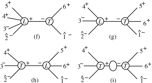
Figure 7: Non-vanishing recursive diagrams. Diagram (i) is the factorization-function contribution.

Next we evaluate the recursive diagrams for the ${[1,2\rangle}$ shift. The diagrams shown in fig. 6 vanish,

$$D_{6}^{\rm(a)}=D_{6}^{\rm(b)}=D_{6}^{\rm(c)}=D_{6}^{\rm(d)}=D_{6}^{\rm(e)}=0\,.$$ (40)

The first two diagrams, 6(a) and 6(b), vanish because the loop vertices $R_{3}(6^{+},1^{-},\hat{K}^{\pm})$ vanish, as mentioned in footnote * ‣ 4.2. Diagrams 6(c) and 6(d) vanish because

$$A_{3}^{\rm tree}(6^{+},\hat{1}^{-},-{\hat{K}}_{61}^{+})\propto\vphantom{\hat{K}}\left[\smash{6}\,\smash{{\hat{K}}_{61}}\right]^{3}=0\,,\hskip 42.67912ptA_{3}^{\rm tree}(\hat{2}^{-},3^{-},-{\hat{K}}_{23}^{+})\propto\vphantom{\hat{K}}\left\langle\smash{\hat{2}}\,\smash{3}\right\rangle^{3}=0\,.$$ (41)

We assume that diagram 6(e) vanishes because its loop vertex is of the same form as the corresponding tree vertex in diagram (d). For a more extensive discussion of this point we refer to ref. [2].

There are four non-vanishing recursive diagrams,

$$R^{D}_{6}=D^{\rm(f)}+D^{\rm(g)}+D^{\rm(h)}+D^{\rm(i)}\,,$$ (42)

shown in fig. 7. A list of vertices that enter the recursion can be found in the appendix of ref. [2]. The recursive diagrams are given by,

$$D_{6}^{\rm(f)} = A_{3}^{\rm tree}(\hat{1}^{-},-\hat{K}_{61}^{-},6^{+})\,{i\over s_{61}}\,R_{5}(\hat{2}^{-},3^{-},4^{+},5^{+},\hat{K}_{61}^{+})$$ (43)

$$= -i\biggl{(}{1\over 3\epsilon}+{8\over 9}\biggr{)}{{\left\langle\smash{3}{\vphantom{1}}^{-}\right|{(1+2)}\left|\smash{6}{\vphantom{1}}^{-}\right\rangle}^{3}\over\left[1\,2\right]\left\langle 3\,4\right\rangle\left\langle 4\,5\right\rangle\left[6\,1\right]\,s_{345}\,\left\langle\smash{5}{\vphantom{1}}^{-}\right|{(3+4)}\left|\smash{2}{\vphantom{1}}^{-}\right\rangle}$$

$$\hbox{}-{i\over 6}\,{s_{345}+s_{34}\over s_{34}s_{345}(s_{345}-s_{34})^{2}}{\left\langle 3\,5\right\rangle\left[4\,5\right]\left[5\,6\right]\left\langle\smash{5}{\vphantom{1}}^{-}\right|{(1+2)}\left|\smash{6}{\vphantom{1}}^{-}\right\rangle\over\left[1\,2\right]\left\langle 4\,5\right\rangle\left[6\,1\right]\,\left\langle\smash{5}{\vphantom{1}}^{-}\right|{(3+4)}\left|\smash{2}{\vphantom{1}}^{-}\right\rangle}$$

$$\hskip 28.45274pt\times(\left\langle\smash{3}{\vphantom{1}}^{-}\right|{4}\left|\smash{5}{\vphantom{1}}^{-}\right\rangle\left\langle\smash{5}{\vphantom{1}}^{-}\right|{(1+2)}\left|\smash{6}{\vphantom{1}}^{-}\right\rangle+\left\langle\smash{3}{\vphantom{1}}^{-}\right|{5}\left|\smash{6}{\vphantom{1}}^{-}\right\rangle s_{345})$$

$$\hbox{}+{i\over 3}\,{{\left[4\,6\right]}^{3}\left\langle\smash{4}{\vphantom{1}}^{-}\right|{(3+5)}\left|\smash{2}{\vphantom{1}}^{-}\right\rangle\over\left[1\,2\right]\left[2\,3\right]\left[3\,4\right]\left\langle 4\,5\right\rangle\left[6\,1\right]\,\left\langle\smash{5}{\vphantom{1}}^{-}\right|{(3+4)}\left|\smash{2}{\vphantom{1}}^{-}\right\rangle}+{i\over 3}\,{{\left[4\,6\right]}^{2}\left\langle\smash{3}{\vphantom{1}}^{-}\right|{(1+2)}\left|\smash{6}{\vphantom{1}}^{-}\right\rangle\over\left[1\,2\right]\left[3\,4\right]\left\langle 4\,5\right\rangle\left[6\,1\right]\,\left\langle\smash{5}{\vphantom{1}}^{-}\right|{(3+4)}\left|\smash{2}{\vphantom{1}}^{-}\right\rangle}$$

$$\hbox{}-{i\over 6}\,{\left\langle 3\,5\right\rangle\left[4\,5\right]\left[5\,6\right]\left\langle\smash{3}{\vphantom{1}}^{-}\right|{(1+2)}\left|\smash{6}{\vphantom{1}}^{-}\right\rangle\left\langle\smash{5}{\vphantom{1}}^{-}\right|{(1+2)}\left|\smash{6}{\vphantom{1}}^{-}\right\rangle\over\left[1\,2\right]\left\langle 4\,5\right\rangle\left[6\,1\right]\,s_{34}s_{345}\,\left\langle\smash{5}{\vphantom{1}}^{-}\right|{(3+4)}\left|\smash{2}{\vphantom{1}}^{-}\right\rangle}\,,$$

$$D^{\rm(g)} = \,A_{4}^{\rm tree}(\hat{2}^{-},3^{-},4^{+},\hat{K}_{561}^{+})\,{i\over s_{561}}R_{4}(\hat{1}^{-},-\hat{K}_{561}^{-},5^{+},6^{+})$$ (44)

$$= \biggl{(}{1\over 3\epsilon}+{8\over 9}\biggr{)}A_{4}^{\rm tree}(\hat{2}^{-},3^{-},4^{+},\hat{K}_{561}^{+})\,{i\over s_{561}}\,A_{4}^{\rm tree}(\hat{1}^{-},-\hat{K}_{561}^{-},5^{+},6^{+})$$

$$= i\biggl{(}{1\over 3\epsilon}+{8\over 9}\biggr{)}{{\left\langle\smash{1}{\vphantom{1}}^{-}\right|{(2+3)}\left|\smash{4}{\vphantom{1}}^{-}\right\rangle}^{3}\over\left[2\,3\right]\left[3\,4\right]\left\langle 5\,6\right\rangle\left\langle 6\,1\right\rangle\,s_{234}\,\left\langle\smash{5}{\vphantom{1}}^{-}\right|{(3+4)}\left|\smash{2}{\vphantom{1}}^{-}\right\rangle}\,,$$

$$D^{\rm(h)} = -D^{\rm(i)}=D^{\rm(g)}\,.$$ (45)

Diagram 7(i) contains the factorization function contribution [15], which for the scalar loop case amounts to a vacuum polarization insertion. The fact that diagrams 7(g), (h) and (i) are equal, up to signs, is rather special to this amplitude.

5.5 Step 5: The Auxiliary Recursion Relation

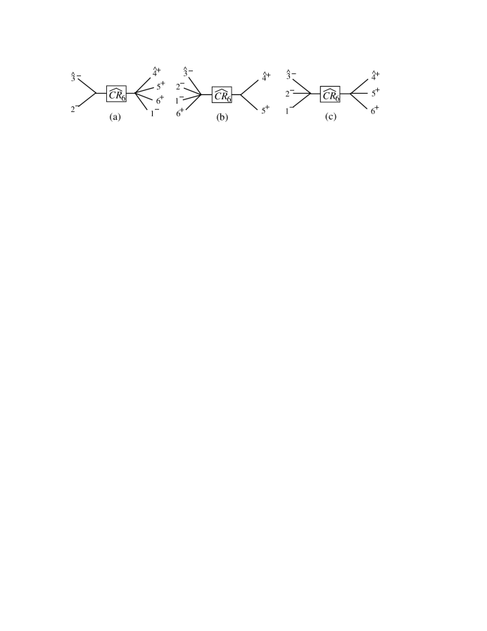
Figure 8: The overlap diagrams arising from an auxiliary ${[3,4\rangle}$ shift in $A^{{\cal N}=0}_{6;1}(1^{-},2^{-},3^{-},4^{+},5^{+},6^{+})$.

Figure 9: The recursive diagrams arising from an auxiliary ${[3,4\rangle}$ shift in $A^{{\cal N}=0}_{6;1}(1^{-},2^{-},3^{-},4^{+},5^{+},6^{+})$. Diagram (c) has non-standard complex singularities.

The diagrams contributing to the overlap and direct recursion from the auxiliary ${[3,4\rangle}$ shift are shown in figs. 8 and 9.

It turns out that in this case the large-parameter behavior under the primary shift of the overlap contribution from the auxiliary shift cancels against that of the cut-completed part,

$$\mathop{\rm Inf}\limits_{{[1,2\rangle}}{{\widehat{C}}_{6}(1^{-},2^{-},3^{-},4^{+},5^{+},6^{+})}+\mathop{\rm Inf}\limits_{{[1,2\rangle}}{O_{6}^{{[3,4\rangle}}(1^{-},2^{-},3^{-},4^{+},5^{+},6^{+})}=0\,.$$ (46)

Furthermore, $\mathop{\rm Inf}\limits_{{[3,4\rangle}}{{\widehat{C}}_{6}}$ vanishes according to eq. (36). The only remaining contribution comes from the direct recursive diagrams. This simplification, however, does not occur in general, and an example where all the aforementioned terms contribute can be found in ref. [2].

Diagram (c) in fig. 9 has non-standard complex singularities. However, according to eq. (29), we only need to keep contributions that are non-vanishing under the primary ${[1,2\rangle}$ shift. It turns out that here only diagram (d) of fig. 9 contributes:

$$\mathop{\rm Inf}\limits_{{[1,2\rangle}}{A_{6;1}^{{\cal N}=0}(1^{-},2^{-},3^{-},4^{+},5^{+},6^{+})}=\mathop{\rm Inf}\limits_{{[1,2\rangle}}{R(1^{-},2^{-},\hat{3}^{-},\hat{K}_{45}^{+},6^{+})}{i\over s_{45}}A_{3}^{\rm tree}(-\hat{K}_{45}^{-},\hat{4}^{+},5^{+})\,,$$ (47)

where the hatted momenta denote momenta shifted under the auxiliary ${[3,4\rangle}$ shift with $w$ frozen to the value

$$w^{\rm(d)}=-{\left\langle 4\,5\right\rangle\over\left\langle 3\,5\right\rangle}\,.$$ (48)

We obtain

$$\mathop{\rm Inf}\limits_{{[1,2\rangle}}{A^{{\cal N}=0}_{6;1}(1^{-},2^{-},3^{-},4^{+},5^{+},6^{+})}=i\,{c_{\Gamma}\over 3}{\left\langle 1\,3\right\rangle^{3}\left\langle 2\,6\right\rangle\over\left\langle 1\,6\right\rangle^{2}\left\langle 3\,4\right\rangle\left\langle 4\,5\right\rangle\left\langle 5\,6\right\rangle\left[1\,2\right]}\,.$$ (49)

5.6 Step 6: Adding Up All Contributions

Upon adding up all contributions, eqs. (31), (35), (37), (42), and (49), following eq. (29), we obtain the final result for the amplitude,

$$A^{{\cal N}=0}_{6;1}(1^{-},2^{-},3^{-},4^{+},5^{+},6^{+})=c_{\Gamma}\Bigl{[}{\widehat{C}}_{6}(1^{-},2^{-},3^{-},4^{+},5^{+},6^{+})+{\widehat{R}}_{6}(1^{-},2^{-},3^{-},4^{+},5^{+},6^{+})\Bigr{]}\,,$$ (50)

where ${\widehat{C}}_{6}(1^{-},2^{-},3^{-},4^{+},5^{+},6^{+})$ is given in eq. (31), and

$${\widehat{R}}_{6}(1^{-},2^{-},3^{-},4^{+},5^{+},6^{+})={\widehat{R}}_{6}^{a}+{\widehat{R}}^{a}_{6}\Bigr{|}_{\rm flip\;1}\,,$$ (51)

where

$${\widehat{R}}_{6}^{a} = {i\over 6}{1\over\left[2\,3\right]\left\langle 5\,6\right\rangle\,\left\langle\smash{5}{\vphantom{1}}^{-}\right|{(3+4)}\left|\smash{2}{\vphantom{1}}^{-}\right\rangle}\Biggl{\{}-{{\left[4\,6\right]}^{3}\left[2\,5\right]\left\langle 5\,6\right\rangle\over\left[1\,2\right]\left[3\,4\right]\left[6\,1\right]}-{{\left\langle 1\,3\right\rangle}^{3}\left\langle 2\,5\right\rangle\left[2\,3\right]\over\left\langle 3\,4\right\rangle\left\langle 4\,5\right\rangle\left\langle 6\,1\right\rangle}$$

$$\hskip 28.45274pt\hbox{}+{{\left\langle\smash{1}{\vphantom{1}}^{-}\right|{(2+3)}\left|\smash{4}{\vphantom{1}}^{-}\right\rangle}^{2}\over\left[3\,4\right]\left\langle 6\,1\right\rangle}\biggl{(}{\left\langle\smash{1}{\vphantom{1}}^{-}\right|{2}\left|\smash{4}{\vphantom{1}}^{-}\right\rangle-\left\langle\smash{1}{\vphantom{1}}^{-}\right|{5}\left|\smash{4}{\vphantom{1}}^{-}\right\rangle\over s_{234}}+{\left\langle 1\,3\right\rangle\over\left\langle 3\,4\right\rangle}-{\left[4\,6\right]\over\left[6\,1\right]}\biggl{)}$$

$$\hskip 28.45274pt\hbox{}-{{\left\langle 1\,3\right\rangle}^{2}(3\left\langle\smash{1}{\vphantom{1}}^{-}\right|{2}\left|\smash{4}{\vphantom{1}}^{-}\right\rangle+\left\langle\smash{1}{\vphantom{1}}^{-}\right|{3}\left|\smash{4}{\vphantom{1}}^{-}\right\rangle)\over\left\langle 3\,4\right\rangle\left\langle 6\,1\right\rangle}+{{\left[4\,6\right]}^{2}(3\left\langle\smash{1}{\vphantom{1}}^{-}\right|{5}\left|\smash{4}{\vphantom{1}}^{-}\right\rangle+\left\langle\smash{1}{\vphantom{1}}^{-}\right|{6}\left|\smash{4}{\vphantom{1}}^{-}\right\rangle)\over\left[3\,4\right]\left[6\,1\right]}\Biggr{\}}\,.\hskip 28.45274pt$$

The result (51) is manifestly symmetric, not only under the flip (30), but also under the second flip symmetry, involving spinor conjugation,

$$X(1,2,3,4,5,6)\Bigr{|}_{\rm flip\ 2}\equiv X^{*}(6,5,4,3,2,1).$$ (53)

6 Summary and Outlook

Above, we have presented a method for the computation of one-loop multi-gluon amplitudes that combines information from unitarity, to determine the cut containing, (poly)logarithmic terms of the amplitude, and factorization, to obtain the rational remainder via on-shell recursion relations. Although the construction of on-shell recursion relations is hindered by several obstacles at the one-loop level, our bootstrap method systematically bypasses these. The method is valid for arbitrary helicity configurations, and relies only on general properties of the gauge theory. We are therefore optimistic that it can be extended to include fermions, and massive partons.

In certain cases, the on-shell recursion relations can be solved explicitly [5]. All-multiplicity results have been obtained for several multi-gluon amplitudes, with all helicities positive or all but one helicity positive [1], for MHV amplitudes [3, 4], and for split-helicity configurations with three adjacent negative helicities and the remainder of positive helicity [2]. The study of the properties of these all-multiplicity amplitudes may reveal some more hidden structure of the underlying gauge theory.

Of course, the aforementioned work is just a starting point. As said above, it is desirable to extend the method to partons other than gluons, as well as fully automatize the computations. Furthermore, a better understanding of complex factorization properties in the non-standard channels would definitely be useful and might even lead to the applicability of recursion relations to higher loop order.

“One of the most remarkable discoveries in elementary particle physics has been that of the existence of the complex plane.”

from J. Schwinger [18] (1970)

Acknowledgements

I thank Zvi Bern, Lance Dixon, Darren Forde, and David Kosower for a very fruitful collaboration. I would also like to thank the conveners of CAQCD06, SUSY06, the Loopfest V, and VLCW06 for inviting me to very stimulating and interesting meetings.

Due to lack of space and due to the vast amount of literature on this topic, the list of references below is necessarily incomplete. A more complete list can be found in [2, 3].

References

- [1] Z. Bern, L. J. Dixon and D. A. Kosower, Phys. Rev. D 71, 105013 (2005) [hep-th/0501240]; Phys. Rev. D 72, 125003 (2005) [hep-ph/0505055]; Phys. Rev. D 73, 065013 (2006) [hep-ph/0507005].
- [2] C. F. Berger, Z. Bern, L. J. Dixon, D. Forde and D. A. Kosower, to appear in Phys. Rev. D (2006) [hep-ph/0604195].
- [3] C. F. Berger, Z. Bern, L. J. Dixon, D. Forde and D. A. Kosower, hep-ph/0607014.
- [4] D. Forde and D. A. Kosower, Phys. Rev. D 73, 061701 (2006) [hep-ph/0509358].
- [5] D. Forde, hep-ph/0608029.
- [6] L. J. Dixon, in QCD & Beyond: Proceedings of TASI ’95, ed. D. E. Soper (World Scientific, 1996) [hep-ph/9601359].
- [7] Z. Bern, L. J. Dixon and D. A. Kosower, Phys. Rev. Lett. 70, 2677 (1993) [hep-ph/9302280].
- [8] R. Britto, F. Cachazo and B. Feng, Nucl. Phys. B 715, 499 (2005) [hep-th/0412308].
- [9] R. Britto, F. Cachazo, B. Feng and E. Witten, Phys. Rev. Lett. 94, 181602 (2005) [hep-th/0501052].
- [10] F. Cachazo and P. Svrcek, PoS RTN2005, 004 (2005) [hep-th/0504194].
- [11] Bootstrapping. In Wikipedia, The Free Encyclopedia. Retrieved July 27, 2006, from http://en.wikipedia.org/w/index.php?title=Bootstrapping&oldid=66160913.
- [12] J. Bedford, A. Brandhuber, B. J. Spence and G. Travaglini, Nucl. Phys. B 712, 59 (2005) [hep-th/0412108].
- [13] Z. Bern, N. E. J. Bjerrum-Bohr, D. C. Dunbar and H. Ita, JHEP 0511, 027 (2005) [hep-ph/0507019].
- [14] R. Britto, B. Feng and P. Mastrolia, Phys. Rev. D 73, 105004 (2006) [hep-ph/0602178].
- [15] Z. Bern and G. Chalmers, Nucl. Phys. B 447, 465 (1995) [hep-ph/9503236].
- [16] R. K. Ellis, W. T. Giele and G. Zanderighi, JHEP 0605, 027 (2006) [hep-ph/0602185].
- [17] Z. G. Xiao, G. Yang and C. J. Zhu, hep-ph/0607017.
- [18] J. Schwinger, Particles, Sources, and Fields, Volume 1, Reading, MA, 1970.