Refined gluino and squark pole masses beyond leading order

Abstract

The physical pole and running masses of squarks and gluinos have recently been related at two-loop order in a mass-independent renormalization scheme. I propose a general method for improvement of such formulas, and argue that better accuracy results. The improved version gives an imaginary part of the pole mass that agrees exactly with the direct calculation of the physical width at next-to-leading order. I also find the leading three-loop contributions to the gluino pole mass in the case that squarks are heavier, using effective field theory and renormalization group methods. The efficacy of these improvements for the gluino and squarks is illustrated with numerical examples. Some necessary three-loop results for gauge coupling and fermion mass beta functions and pole masses in theories with more than one type of fermion representation, which are not directly accessible from the published literature, are presented in an Appendix.

I Introduction

The small ratio of the electroweak symmetry breaking scale to the Planck mass can be stabilized quadscancel in softly-broken supersymmetric extensions of the Standard Model. This implies that all of the Standard Model particles will have superpartners, which should be within reach of the $p\overline{p}$ Fermilab Tevatron collider or the $pp$ Large Hadron Collider during the next few years. Most of the new parameters appearing in the Minimal Supersymmetric Standard Model (MSSM) Martin:1997ns are the masses of the new superpartners and other supersymmetry-breaking couplings of positive mass dimension. Therefore, a detailed understanding of the MSSM Lagrangian is nearly synonymous with an understanding of supersymmetry breaking.

The fact that experimental observations of flavor violation and CP violation are not in significant disagreement with the predictions of the Standard Model can be taken as indirect evidence for the existence of some powerful organizing principle governing supersymmetry breaking and its mediation to the MSSM sector. An especially interesting possibility is that the organizing principle can be discerned by running the parameters of the theory up to high energy scales using the renormalization group. To carry out this analysis, it will be crucial to relate physically measured observables, especially the superpartner masses, to running parameters in the full theory defined by the non-decoupled Lagrangian that includes all of the superpartners.

However, running masses are not the most direct observables expected from collider experiments. In general, the mass defined by the position of the complex pole in the propagator is a gauge-invariant and renormalization scale-invariant quantity Tarrach:1980up -Gambino:1999ai . The pole mass does suffer from ambiguities poleambiguities due to infrared physics associated with the QCD confinement scale, but these are probably not large enough to cause a practical problem for strongly-interacting superpartners. The complex pole mass should be closely related in a calculable way to the kinematic observable mass and width reported by experiments massdefs .

It is often useful to calculate in on-shell schemes, in which some physical masses and other observables are used as input data and others are outputs. However, for the key purpose of unraveling the organizing principle behind the supersymmetry-breaking Lagrangian, this is not as directly useful. The $\overline{\rm MS}$ scheme MSbar can also be used, but it violates supersymmetry explicitly. Instead, it is preferable to use the $\overline{\rm DR}$ scheme DRbar (or the revised $\overline{\rm DR}^{\prime}$ scheme DRbarprime , which removes the unphysical effects of epsilon-scalar masses in softly-broken supersymmetric models), with all superpartners non-decoupled. While it is difficult to know in detail what limitations on this program will follow from future experimental uncertainties, it seems clear that multi-loop calculations will be necessary to make the theoretical sources of error negligible.

The one-loop relations between the superpartner pole masses and the running parameters in the MSSM Lagrangian have been known for some time Martin:1993yx -PBMZ . The calculation of the Higgs scalar boson masses in the MSSM has now advanced to include the important two-loop corrections (for some reviews of recent progress, see Degrassi:2002fi -Heinemeyer:2004ms ), and even some three-loop corrections Degrassi:2002fi , using a variety of different methods. Recent calculations have provided the supersymmetric QCD (SUSYQCD) two-loop corrections to the squark Martin:2005eg and gluino Yamada:2005ua ; Martin:2005ch masses. The quark masses in the MSSM are known at two-loop order quarkpoleSUSY ,Martin:2005ch . More generally, refs. Martin:2005eg and Martin:2005ch provide the self-energy functions and pole masses for scalars and fermions, respectively, calculated in mass-independent renormalization schemes at two-loop order in any renormalizable field theory, in the approximation that vector bosons are treated as massless in the two-loop parts. This approximation is likely to be quite good for most applications to the MSSM, because the largest two-loop effects involving vector bosons come from SUSYQCD, and because the $W$ and $Z$ bosons are evidently lighter than most of the superpartners.

It is important to consider the validity of the perturbative expansion in these results. Especially for the lightest Higgs boson, the squarks, and the gluino, the corrections that give the pole masses from the running masses turn out to be quite significant. As a prominent example, even the pure two-loop correction to the gluino mass (compared to the running mass evaluated at a renormalization group scale equal to itself) is of order 1-2% in the case that squarks and gluinos are comparable in mass, and grows to about 5% for squark masses that are of order 5 times heavier than the gluino. One would like some assurance that perturbation theory is really converging, and an estimate of the theoretical error. Unfortunately, the renormalization-scale dependence of these results is not a reliable error estimate; in particular, the scale dependence of one-loop corrections is routinely much smaller than the two-loop corrections when the latter are known.

Another reason to be wary is the fact that calculations in mass-independent renormalization schemes like $\overline{\rm MS}$ or $\overline{\rm DR}^{\prime}$ use propagators with masses that can differ significantly from the physical ones. In many cases this is true for any reasonable choice of the renormalization scale $Q$. A troubling aspect of this is that the imaginary part of the complex pole squared mass,

$$s_{\rm pole}=M^{2}-i\Gamma M$$ (1.1)

can give a numerical value for the width $\Gamma$ that differs quite badly from the physical width. It is not hard to find examples for which the tree-level masses are sufficiently different from the physical masses that a particular contribution to $\Gamma$ as computed from the complex pole mass is exactly 0 (because the decay would be kinematically forbidden if the particles had masses equal to the tree-level Lagrangian masses appearing in the propagators of the self-energy loop diagrams), while the true decay width contribution (computed directly from diagrams with multi-particle final states, using an on-shell scheme) is non-zero. Or, the reverse can happen. (I will show an example of each type in Figure 2 of section IV.) While the complex pole mass is in principle a gauge-invariant and renormalization-scale invariant observable, this calls into question how well one can trust the perturbation theory that yields it in practice.

These issues are general. However, in the MSSM, they are particularly acute for the squarks and the gluino, because of their strong coupling. Furthermore, the LHC will quite likely produce gluinos and squarks in abundance if supersymmetry is correct. Therefore, I will use the squark and gluino SUSYQCD system within the MSSM as an example in this paper to show how to ameliorate the problems mentioned above. First, in section 2, I discuss how to reorganize the results of perturbation theory by expanding tree-level masses around physical masses in the loop corrections obtained in mass-independent ($\overline{\rm MS}$ or $\overline{\rm DR}^{\prime}$) schemes. In section 3, I present a result for the three-loop corrections to the gluino mass, valid in the limit that squarks are treated as nearly degenerate and much heavier than the gluino. This is the case where one might expect three-loop and even higher-order corrections to be most dangerous, but I show that they are actually under good control, and can be tamed by using effective field theory and renormalization group methods. Section 4 displays some numerical results showing the efficacy of these improvements. In an Appendix, I present some necessary results for three-loop contributions to fermion mass beta functions and pole masses in (non-supersymmetric) theories with fermions in distinct representations.

II Improved two-loop pole mass results

In general, the two-loop order expression for the pole mass of a particle can be computed from knowledge of the self-energy function,

$$\Pi_{j}^{k}(s)=\frac{1}{16\pi^{2}}\Pi^{(1)k}_{j}+\frac{1}{(16\pi^{2})^{2}}\Pi^{(2)k}_{j}+\ldots,$$ (2.1)

Here $s$ is the external momentum invariant, the superscript in parentheses indicates the loop order, and the indices $j,k$ indicate different particles with the same quantum numbers, which in general can mix. For fermions, $\Pi_{j}^{k}(s)$ can be assembled from separate chirality-preserving and chirality-violating self-energy functions, as described in section II.C of ref. Martin:2005ch . Then the gauge-invariant and renormalization-scale invariant pole squared masses can be defined formally as the solutions to the equation

$${\rm Det}[(s-m_{j}^{2})\delta_{j}^{k}-\Pi_{j}^{k}(s)]=0,$$ (2.2)

where $m_{i}^{2}$ are the tree-level diagonalized squared masses. However, because $\Pi_{j}^{k}$ should be interpreted as a complex-valued function of a real variable $s$, this equation must be solved by first expanding the self-energy function as a series about a point on the real $s$-axis. In evaluating the loop integrals in the self-energy, $s$ is given a positive infinitesimal imaginary part, while the complex pole squared mass solution [see eq. (1.1)] always has a non-positive imaginary part. A related subtlety is that when the particle in question has couplings to massless gauge bosons, terms of a given loop order in the self-energy have branch-cut singularities (except when the Fried-Yennie gauge-fixing condition is used PasseraSirlin ; Martin:2005eg ).

The most straightforward way to obtain the pole mass at two-loop order in a mass-independent renormalization scheme is to first expand $\Pi_{j}^{k}(s)$ in a series about the tree-level squared masses. Define, for a generic squared mass $m^{2}$:

$$\widetilde{\Pi}_{j}^{(1)k}(m^{2}) \equiv \lim_{s\rightarrow m^{2}+i\varepsilon}\Pi^{(1)k}_{j}(s),$$ (2.3)

$$\widetilde{\Pi}_{j}^{(2)j}(m^{2}) \equiv \lim_{s\rightarrow m^{2}+i\varepsilon}\left[\Pi^{(2)j}_{j}(s)+\Pi_{j}^{(1)j}(s)\frac{\partial}{\partial s}\Pi_{j}^{(1)j}(s)\right],$$ (2.4)

where the self-energy functions on the right-hand side are computed in a mass-independent renormalization scheme, and no sum on $j$ is implied in eq. (2.4). Then, working consistently to two-loop order, the pole mass for the particle with tree-level squared mass $m^{2}_{j}$ is

$$M_{j}^{2}-i\Gamma_{j}M_{j} = m_{j}^{2}+\frac{1}{16\pi^{2}}\widetilde{\Pi}_{j}^{(1)j}(m_{j}^{2})+\frac{1}{(16\pi^{2})^{2}}\Bigl{\{}\widetilde{\Pi}_{j}^{(2)j}(m_{j}^{2})+\sum_{k\not=j}\widetilde{\Pi}_{j}^{(1)k}(m_{j}^{2})\widetilde{\Pi}_{k}^{(1)j}(m_{j}^{2})/(m_{j}^{2}-m_{k}^{2})\Bigr{\}},$$ (2.5)

obtained by a perturbative expansion of eq. (1.1).

The previous expression is gauge-invariant, and renormalization scale invariant up to terms of three-loop order. In its application to the squark and gluino masses in the MSSM, this approach has the advantage of depending only on tree-level running parameters, so that iteration is not necessary if they are taken as given. However, as remarked in the Introduction, the use of tree-level running masses in propagators is problematic at least for the imaginary part of the pole mass, which arises from the absorptive part of the self-energy functions. If the tree-level masses differ significantly from the physical masses of the particles, then the kinematics of the self-energy functions will poorly reflect the actual kinematics giving rise to the physical width of the particle. This can lead to a non-zero width when there should be none, or vice versa. In general, one may care more about the real part of the pole mass, but intuitively one cannot expect the real part to be very accurate if the kinematics in the loop integrations poorly reflects the physical particle masses, and if the imaginary part is completely wrong.

To improve the situation, let us reorganize the previous result by expanding all tree-level squared masses appearing in the $\widetilde{\Pi}$ functions in a series about the real parts of their respective pole squared masses. (Note that although I have written the $\widetilde{\Pi}$ functions as depending on a single external squared mass argument that replaced $s$, there is also dependence on the internal propagator masses which is not explicitly indicated.) Doing this, one arrives at:

$$M_{j}^{2}-i\Gamma_{j}M_{j} = m_{j}^{2}+\frac{1}{16\pi^{2}}\overline{\Pi}_{j}^{(1)j}(M_{j}^{2})+\frac{1}{(16\pi^{2})^{2}}\Bigl{\{}\overline{\Pi}_{j}^{(2)j}(M_{j}^{2})+\sum_{k\not=j}\overline{\Pi}_{j}^{(1)k}(M_{j}^{2})\overline{\Pi}_{k}^{(1)j}(M_{j}^{2})/(M_{j}^{2}-M_{k}^{2})$$ (2.6)

$$-\sum_{k}{\rm Re}\bigl{[}\overline{\Pi}_{k}^{(1)k}(M_{k}^{2})\bigr{]}\frac{\partial}{\partial M_{k}^{2}}\overline{\Pi}_{j}^{(1)j}(M_{j}^{2})\Bigr{\}},$$

The second sum over $k$ is taken over all fermions and bosons in the theory that couple to particle $j$, not just those that can mix with $j$. The $\overline{\Pi}$ in eq. (2.6) are defined to have the same functional dependence on the real parts of the pole squared masses (both external and internal) as the functions $\widetilde{\Pi}$ in eq. (2.5) did on the tree-level squared masses. Because the one-loop and two-loop parts of eq. (2.5) are each separately gauge-fixing invariant, it is clear that eq. (2.6) is also independent of gauge-fixing. Formally, eqs. (2.5) and (2.6) are equivalent up to terms of three-loop order. However, in eq. (2.6), all kinematic dependences of loop integrals on the right-hand side correspond to the physical masses (the real parts of the pole masses). I therefore expect that, when it makes much of a difference, eq. (2.6) should be more accurate than eq. (2.5). If one starts with the Lagrangian parameters as input, evaluation of the pole masses will require an iterative procedure involving all of the particle masses simultaneously, which in a general case at two-loop order could take a significant computation time. On the other hand, if physical masses are taken as inputs, eq. (2.6) still requires knowledge of the tree-level couplings and mixing matrices of the theory. The one-loop functions are always known analytically in terms of logarithms, so taking derivatives of them poses no technical difficulties. The two-loop functions often cannot be computed analytically, but computer codes such as TSIL TSIL provide for their numerical computation.

To illustrate the method, I choose here to consider the two-loop corrections to the gluino and squark pole masses, for simplicity including only SUSYQCD corrections and ignoring the effects of squark mixing, quark masses, and electroweak effects. For this system, the realization of eq. (2.5) is:

$$\!\!\!\!\!\!\!\!\!\!\!\!M_{\tilde{Q}_{j}}^{2}-i\Gamma_{\tilde{Q}_{j}}M_{\tilde{Q}_{j}}\>=\>m_{\tilde{Q}_{j}}^{2}+hC_{q}\widetilde{\Pi}_{\tilde{Q}}^{(1)}(m_{\tilde{Q}_{j}}^{2},m_{\tilde{g}}^{2})+h^{2}C_{q}\Bigl{[}C_{q}\widetilde{\Pi}_{\tilde{Q}}^{(2,a)}(m_{\tilde{Q}_{j}}^{2},m_{\tilde{g}}^{2})+C_{A}\widetilde{\Pi}_{\tilde{Q}}^{(2,b)}(m_{\tilde{Q}_{j}}^{2},m_{\tilde{g}}^{2})$$

$$\qquad\qquad\qquad\quad+I_{q}\sum_{k}\widetilde{\Pi}_{\tilde{Q}}^{(2,c)}(m_{\tilde{Q}_{j}}^{2},m_{\tilde{g}}^{2},m_{\tilde{Q}_{k}}^{2})\Bigr{]},$$ (2.7)

$$\!\!\!\!\!\!\!\!\!\!\!\!M_{\tilde{g}}^{2}-i\Gamma_{\tilde{g}}M_{\tilde{g}}\>=\>m_{\tilde{g}}^{2}+h\Bigl{[}C_{A}\widetilde{\Pi}_{\tilde{g}}^{(1,a)}(m_{\tilde{g}}^{2})+I_{q}\sum_{j}\widetilde{\Pi}_{\tilde{g}}^{(1,b)}(m_{\tilde{g}}^{2},m_{\tilde{Q}_{j}}^{2})\Bigr{]}+h^{2}\Bigl{[}C_{A}^{2}\widetilde{\Pi}_{\tilde{g}}^{(2,a)}(m_{\tilde{g}}^{2})$$

$$\qquad\qquad\quad+C_{A}I_{q}\sum_{j}\widetilde{\Pi}_{\tilde{g}}^{(2,b)}(m_{\tilde{g}}^{2},m_{\tilde{Q}_{j}}^{2})+C_{q}I_{q}\sum_{j}\widetilde{\Pi}_{\tilde{g}}^{(2,c)}(m_{\tilde{g}}^{2},m_{\tilde{Q}_{j}}^{2})+I_{q}^{2}\sum_{j}\sum_{k}\widetilde{\Pi}_{\tilde{g}}^{(2,d)}(m_{\tilde{g}}^{2},m_{\tilde{Q}_{j}}^{2},m_{\tilde{Q}_{k}}^{2})\Bigr{]}.$$ (2.8)

Here, $m_{\tilde{g}}^{2}$ and $m_{\tilde{Q}_{j}}^{2}$ are the tree-level $\overline{\rm DR}^{\prime}$ squared masses. In many references, $m_{\tilde{g}}$ is written as $M_{3}$, but in the present paper, capital letters are reserved for pole masses and lowercase letters for running masses. The strong gauge coupling appears in the combination:

$$h\>\equiv\>{g_{3}^{2}}/{16\pi^{2}}\>=\>\alpha_{S}/4\pi.$$ (2.9)

The indices $j$ and $k$ run over the 12 squark mass eigenstates of the MSSM (taken here to be unmixed, but not necessarily degenerate), and for $SU(3)_{c}$, $C_{A}=3$ and $C_{q}=4/3$ and $I_{q}=1/2$. The functions $\widetilde{\Pi}$ appearing in eq. (2.7) were given in eqs. (5.6)-(5.9) of ref. Martin:2005eg , and those in eq. (2.8) were given in eqs. (5.5)-(5.10) of ref. Martin:2005ch . Note that the dependence on all squared masses is explicit in the arguments of these functions.

Applying eq. (2.6) to this gives the improved equations for the relation between pole and running squared masses:

$$\!\!\!\!\!\!\!\!\!\!\!\!M_{\tilde{Q}_{j}}^{2}-i\Gamma_{\tilde{Q}_{j}}M_{\tilde{Q}_{j}}\>=\>m_{\tilde{Q}_{j}}^{2}+hC_{q}\widetilde{\Pi}_{\tilde{Q}}^{(1)}(M_{\tilde{Q}_{j}}^{2},M_{\tilde{g}}^{2})+h^{2}C_{q}\Bigl{\{}C_{q}\widetilde{\Pi}_{\tilde{Q}}^{(2,a)}(M_{\tilde{Q}_{j}}^{2},M_{\tilde{g}}^{2})+C_{A}\widetilde{\Pi}_{\tilde{Q}}^{(2,b)}(M_{\tilde{Q}_{j}}^{2},M_{\tilde{g}}^{2})$$

$$\qquad\qquad\qquad\>\>\>+I_{q}\sum_{k}\widetilde{\Pi}_{\tilde{Q}}^{(2,c)}(M_{\tilde{Q}_{j}}^{2},M_{\tilde{g}}^{2},M_{\tilde{Q}_{k}}^{2})-C_{q}{\rm Re}[\widetilde{\Pi}_{\tilde{Q}}^{(1)}(M_{\tilde{Q}_{j}}^{2},M_{\tilde{g}}^{2})]\frac{\partial}{\partial M_{\tilde{Q}_{j}}^{2}}\widetilde{\Pi}_{\tilde{Q}}^{(1)}(M_{\tilde{Q}_{j}}^{2},M_{\tilde{g}}^{2})$$

$$\qquad\qquad\qquad\>\>\>-{\rm Re}\bigl{[}C_{A}\widetilde{\Pi}_{\tilde{g}}^{(1,a)}(M_{\tilde{g}}^{2})+I_{q}\sum_{k}\widetilde{\Pi}_{\tilde{g}}^{(1,b)}(M_{\tilde{g}}^{2},M_{\tilde{Q}_{k}}^{2})\bigr{]}\frac{\partial}{\partial M_{\tilde{g}}^{2}}\widetilde{\Pi}_{\tilde{Q}}^{(1)}(M_{\tilde{Q}_{j}}^{2},M_{\tilde{g}}^{2})\Bigr{\}},$$ (2.10)

$$\!\!\!\!\!\!\!\!\!\!\!\!M_{\tilde{g}}^{2}-i\Gamma_{\tilde{g}}M_{\tilde{g}}\>=\>m_{\tilde{g}}^{2}+h\Bigl{[}C_{A}\widetilde{\Pi}_{\tilde{g}}^{(1,a)}(M_{\tilde{g}}^{2})+I_{q}\sum_{j}\widetilde{\Pi}_{\tilde{g}}^{(1,b)}(M_{\tilde{g}}^{2},M_{\tilde{Q}_{j}}^{2})\Bigr{]}+h^{2}\biggl{\{}C_{A}^{2}\widetilde{\Pi}_{\tilde{g}}^{(2,a)}(M_{\tilde{g}}^{2})$$

$$\qquad\qquad\quad+C_{A}I_{q}\sum_{j}\widetilde{\Pi}_{\tilde{g}}^{(2,b)}(M_{\tilde{g}}^{2},M_{\tilde{Q}_{j}}^{2})+C_{q}I_{q}\sum_{j}\widetilde{\Pi}_{\tilde{g}}^{(2,c)}(M_{\tilde{g}}^{2},M_{\tilde{Q}_{j}}^{2})+I_{q}^{2}\sum_{j}\sum_{k}\widetilde{\Pi}_{\tilde{g}}^{(2,d)}(M_{\tilde{g}}^{2},M_{\tilde{Q}_{j}}^{2},M_{\tilde{Q}_{k}}^{2})$$

$$\qquad\qquad\quad-{\rm Re}\Bigl{[}C_{A}\widetilde{\Pi}_{\tilde{g}}^{(1,a)}(M_{\tilde{g}}^{2})+I_{q}\sum_{k}\widetilde{\Pi}_{\tilde{g}}^{(1,b)}(M_{\tilde{g}}^{2},M_{\tilde{Q}_{k}}^{2})\Bigr{]}\frac{\partial}{\partial M_{\tilde{g}}^{2}}\Bigl{[}C_{A}\widetilde{\Pi}_{\tilde{g}}^{(1,a)}(M_{\tilde{g}}^{2})+I_{q}\sum_{j}\widetilde{\Pi}_{\tilde{g}}^{(1,b)}(M_{\tilde{g}}^{2},M_{\tilde{Q}_{j}}^{2})\Bigr{]}$$

$$\qquad\qquad\quad-C_{q}I_{q}\sum_{j}{\rm Re}\Bigl{[}\widetilde{\Pi}_{\tilde{Q}}^{(1)}(M_{\tilde{Q}_{j}}^{2},M_{\tilde{g}}^{2})\Bigr{]}\frac{\partial}{\partial M_{\tilde{Q}_{j}}^{2}}\widetilde{\Pi}_{\tilde{g}}^{(1,b)}(M_{\tilde{g}}^{2},M_{\tilde{Q}_{j}}^{2})\biggr{\}}.$$ (2.11)

Given the running masses and coupling as inputs, the pole masses can now be solved for iteratively. Or, given the pole masses and the running gauge coupling as inputs, the running masses can be immediately extracted.

I have checked analytically that the imaginary parts of the pole masses given in eqs. (2.10) and (2.11) correspond exactly to the gluino and squark decay widths calculated at next-to-leading order in Beenakker:1996dw . This is a good reason to prefer the improved version eqs. (2.10) and (2.11) over eqs. (2.7) and (2.8), and more generally eq. (2.6) over eq. (2.5). In section IV, I will present a numerical comparison of these equations.

III Three-loop contributions to the gluino pole mass

Radiative corrections to the mass of the gluino in the MSSM are particularly large, for two reasons. First, the gluino is a color octet, and so is effectively more strongly coupled than a quark in the fundamental representation. Second, it couples to 12 squark/quark pairs. If one expresses the gluino pole mass in terms of the running mass evaluated at itself in a non-decoupling scheme, then the squark-mediated corrections are large and grow logarithmically with the ratio of the squark to gluino masses. One can exploit this by using effective field theory and renormalization group methods to obtain the logarithmically-enhanced parts. In this section, I will use this strategy to evaluate the three-loop gluino pole mass in the formal limit $M_{\tilde{Q}}^{2}\gg M_{\tilde{g}}^{2}$, neglecting terms of three-loop order that are suppressed by $M_{\tilde{g}}^{2}/M_{\tilde{Q}}^{2}$, but including all terms of order $L^{3}$, $L^{2}$, and $L$, where

$$L\>\equiv\>\ln(M_{\tilde{Q}}^{2}/M_{\tilde{g}}^{2}).$$ (3.1)

I will also find the coefficient of the $L^{0}$ term, up to a single (presently) unknown and plausibly sub-dominant matching coefficient. This analysis neglects squark mixing and non-degeneracy, electroweak effects, and Standard Model quark masses, for simplicity. The same method could quite easily be extended to include all terms of order

$$\alpha_{S}^{n}L^{n},\>\>\alpha_{S}^{n}L^{n-1},\>\>{\rm and}\>\>\alpha_{S}^{n}L^{n-2},$$ (3.2)

at arbitrary loop order $n$, but the residual unknown three-loop order contributions are likely to be larger than the contributions from $n\geq 4$. In the following, I will use the following convenient notations for other logarithms:

$$L_{\tilde{g}} \equiv \ln(M_{\tilde{g}}^{2}/Q^{2}),$$ (3.3)

$$L_{\tilde{Q}} \equiv \ln(M_{\tilde{Q}}^{2}/Q^{2}),$$ (3.4)

$$\ell \equiv \ln(m_{\tilde{Q}}^{2}/m_{\tilde{g}}^{2}),$$ (3.5)

$$\ell_{\tilde{g}} \equiv \ln(m_{\tilde{g}}^{2}/Q^{2}),$$ (3.6)

$$\ell_{\tilde{Q}} \equiv \ln(m_{\tilde{Q}}^{2}/Q^{2}),$$ (3.7)

where $Q$ is the renormalization group scale, and the running gluino and squark masses in the last three definitions are taken to be in the full theory (with squarks included).

The starting point is the three-loop pole mass for a color octet Majorana fermion ($\tilde{g}$) in the presence of 6 light quark flavors $(u,d,s,c,b,t)$. This is the same fermion content of SUSYQCD as found in ref. slightlysplitsusy and the extreme limit of “split supersymmetry” splitsusy ; it is the effective theory in which squarks have been decoupled. The three-loop gluino pole mass in this model is almost known from ref. Melnikov:2000qh , up to a single ambiguity that is resolved in the Appendix of the present paper. The result can be written as:

$$M_{\tilde{g}} = \widehat{m}_{\tilde{g}}(Q)\Bigl{(}1+\widehat{h}\bigl{[}a^{(1)}_{1}L_{\tilde{g}}+a^{(1)}_{0}\bigr{]}+\widehat{h}^{2}\bigl{[}a^{(2)}_{2}L_{\tilde{g}}^{2}+a^{(2)}_{1}L_{\tilde{g}}+a^{(2)}_{0}\bigr{]}+\widehat{h}^{3}\bigl{[}a^{(3)}_{3}L_{\tilde{g}}^{3}+a^{(3)}_{2}L_{\tilde{g}}^{2}+a^{(3)}_{1}L_{\tilde{g}}+a^{(3)}_{0}\bigr{]}+\ldots\Bigr{)},\phantom{xxx.}$$ (3.8)

where $M_{\tilde{g}}$ is the gluino pole mass, and the hats on the symbols $\widehat{m}_{\tilde{g}}$ and $\widehat{h}\equiv\hat{g}_{3}^{2}/16\pi^{2}$ are used to distinguish the running $\overline{\rm MS}$ parameters in the effective theory without squarks. The coefficients appearing here are:

$$a^{(1)}_{0} = 12,\qquad a^{(1)}_{1}\>=\>-9,$$ (3.9)

$$a^{(2)}_{0} = 339+33\pi^{2}-36\pi^{2}\ln 2+54\zeta_{3},$$ (3.10)

$$a^{(2)}_{1} = -282,\qquad a^{(2)}_{2}\>=\>63,$$ (3.11)

$$a^{(3)}_{0} = 172399/18+73367\pi^{2}/10-12672\pi^{2}\ln 2$$ (3.12)

$$+12330\zeta_{3}-121\pi^{4}/2-48\pi^{2}\ln^{2}2$$

$$+552\ln^{4}2+13248{\rm Li}_{4}(1/2)$$

$$+675\pi^{2}\zeta_{3}-1890\zeta_{5},$$

$$a^{(3)}_{1} = -8932-627\pi^{2}+684\pi^{2}\ln 2-306\zeta_{3},$$ (3.13)

$$a^{(3)}_{2} = 3093,\qquad a^{(3)}_{3}\>=\>-399.$$ (3.14)

Note that in this section, the gluino pole mass is real, because the gluino has no allowed decays in pure SUSYQCD in the case that all squarks are heavier.

The terms in eq. (3.8) that depend on $L_{\tilde{g}}$, and thus explicitly involve the renormalization scale $Q$, are obtained from the renormalization group equations for the gauge coupling and running gluino mass in the effective theory:

$$Q\frac{d}{dQ}\widehat{h} = \widehat{h}^{2}b^{(1)}_{\widehat{h}}+\widehat{h}^{3}b^{(2)}_{\widehat{h}}+\widehat{h}^{4}b^{(3)}_{\widehat{h}}+\ldots$$ (3.15)

$$Q\frac{d}{dQ}\widehat{m}_{\tilde{g}} = \widehat{m}_{\tilde{g}}\bigr{[}\widehat{h}b^{(1)}_{\widehat{m}_{\tilde{g}}}+\widehat{h}^{2}b^{(2)}_{\widehat{m}_{\tilde{g}}}+\widehat{h}^{3}b^{(3)}_{\widehat{m}_{\tilde{g}}}+\ldots\bigr{]},\phantom{xzx}$$ (3.16)

where

$$b^{(1)}_{\widehat{h}} = -10,\qquad b^{(2)}_{\widehat{h}}\>=\>44,$$ (3.17)

$$b^{(3)}_{\widehat{h}} = 4168/3,$$ (3.18)

$$b^{(1)}_{\widehat{m}_{\tilde{g}}} = -18,\qquad b^{(2)}_{\widehat{m}_{\tilde{g}}}\>=\>-228,$$ (3.19)

$$b^{(3)}_{\widehat{m}_{\tilde{g}}} = -2774+1440\zeta_{3}.$$ (3.20)

The last coefficient does not seem to be obtainable directly from the results in the published literature, which only deal with theories with a single type of fermion representation. However, it can be inferred from an unpublished paper of O.V. Tarasov Tarasov:1982gk . This is explained in the Appendix of the present paper.

The results given above are not what is needed in order to discern an organizing principle for supersymmetry breaking. Instead, one needs to obtain the running parameters in the full theory with squarks included. This can be achieved from matching conditions between the effective theory parameters $(\widehat{h},\widehat{m}_{\tilde{g}})$ and the full theory parameters $(h,m_{\tilde{g}},m_{\tilde{Q}}^{2})$. In these equations, the effective theory parameters $(\widehat{h},\widehat{m}_{\tilde{g}})$ are always in $\overline{\rm MS}$, while the full theory parameters $(h,m_{\tilde{g}},m_{\tilde{Q}}^{2})$ are always in the $\overline{\rm DR}^{\prime}$ scheme here. (It may also be possible to use $\overline{\rm DR}$ for the effective theory, but then there are subtleties associated with evanescent couplings in non-supersymmetric theories nonSUSYDRbar .) Now one can take the gluino pole mass from eq. (3.8) and use the matching to rewrite it in terms of the parameters of the full theory. In the approximation used here, non-renormalizable terms are not included in the effective field theory Lagrangian, which corresponds to neglecting all contributions suppressed by powers of $M_{\tilde{g}}^{2}/M_{\tilde{Q}}^{2}$. Experience shows that expansions of radiative corrections in such mass ratios typically converge quite quickly, so I suspect that it is reasonable to hope that the results below will be approximately valid even if the typical squark mass is not very much larger than the gluino mass.

The renormalization group equations for the parameters of the non-decoupled theory are:

$$Q\frac{d}{dQ}h = h^{2}b^{(1)}_{h}+h^{3}b^{(2)}_{h}+h^{3}b^{(3)}_{h}+\ldots$$ (3.21)

$$Q\frac{d}{dQ}m_{\tilde{g}} = m_{\tilde{g}}\bigr{[}hb^{(1)}_{m_{\tilde{g}}}+h^{2}b^{(2)}_{m_{\tilde{g}}}+h^{3}b^{(3)}_{m_{\tilde{g}}}+\ldots\bigr{]}\phantom{xxx}$$ (3.22)

$$Q\frac{d}{dQ}m^{2}_{\widetilde{Q}} = m_{\tilde{g}}^{2}\bigl{[}hb^{(1)}_{m_{\tilde{Q}}^{2}}+h^{2}b^{(2a)}_{m_{\tilde{Q}}^{2}}+\ldots\bigr{]}$$ (3.23)

$$+m^{2}_{\widetilde{Q}}\bigl{[}h^{2}b^{(2b)}_{m_{\tilde{Q}}^{2}}+\ldots\bigr{]}$$

where threeloopgaugeMSSM :

$$b^{(1)}_{h} = -6,\qquad b^{(2)}_{h}\>=\>28,\qquad b^{(3)}_{h}\>=\>694/3,\phantom{\frac{X^{\prime X}}{X^{\prime}_{X}}}$$ (3.24)

and twoloopgauginoMSSM ; threeloopgauginoMSSM :

$$b^{(n)}_{m_{\tilde{g}}} = nb^{(n)}_{h},$$ (3.25)

and DRbarprime ; twoloopsquarkMSSM :

$$b^{(1)}_{m_{\tilde{Q}}^{2}} = -32/3,\qquad b^{(2a)}_{m_{\tilde{Q}}^{2}}\>=\>-128/3,\phantom{X_{X_{X}}}$$ (3.26)

$$b^{(2b)}_{m_{\tilde{Q}}^{2}} = 64.\phantom{\frac{X^{X}}{X^{X}}}$$ (3.27)

The two-loop gauge coupling matching condition has been obtained in ref. Harlander:2005wm :

$$\widehat{h} = h\Bigl{[}1+h\bigl{(}-1+2L_{\tilde{Q}}\bigr{)}+h^{2}\bigl{(}23-12L_{\tilde{Q}}+4L_{\tilde{Q}}^{2}\bigr{)}+\ldots\Bigr{]}.$$ (3.28)

For the gaugino mass matching condition, I find:

$$\widehat{m}_{\tilde{g}} = m_{\tilde{g}}\Bigl{[}1+h\bigl{(}6L_{\tilde{Q}}\bigr{)}+h^{2}\bigl{(}14\pi^{2}/3-176+133L_{\tilde{Q}}+18L_{\tilde{Q}}^{2}\bigr{)}$$ (3.29)

$$+h^{3}\bigl{(}c^{(3)}_{m_{\tilde{g}}}+[1713-720\zeta_{3}]L_{\tilde{Q}}+615L_{\tilde{Q}}^{2}+48L_{\tilde{Q}}^{3}\bigr{)}+\ldots\Bigr{]}.$$

I obtained the two-loop coefficients here by a direct comparison of the two-loop gluino pole squared mass as found in the full theory with $\overline{\rm DR}^{\prime}$ and in the effective theory with $\overline{\rm MS}$, using the results of ref. Martin:2005ch . The three-loop logarithmic terms in eq. (3.29) are obtained from the renormalization group equations (3.15)-(3.27). Unfortunately, the coefficient $c^{(3)}_{m_{\tilde{g}}}$ remains unknown, and seems quite difficult to calculate.

The preceding results can now be used straightforwardly to obtain the three-loop result for the gluino pole mass in terms of the non-decoupled theory parameters. I find:

$$M_{\tilde{g}} = m_{\tilde{g}}(Q)\Bigl{(}1+h\bigr{[}a^{(1)}_{00}+a^{(1)}_{10}L_{\tilde{g}}+a^{(1)}_{01}L_{\tilde{Q}}\bigl{]}+h^{2}\bigr{[}a^{(2)}_{00}+a^{(2)}_{10}L_{\tilde{g}}+a^{(2)}_{01}L_{\tilde{Q}}+a^{(2)}_{20}L_{\tilde{g}}^{2}+a^{(2)}_{11}L_{\tilde{g}}L_{\tilde{Q}}+a^{(2)}_{02}L_{\tilde{Q}}^{2}\bigl{]}$$ (3.30)

$$\!\!\!\!\!\!\!\!\!\!\!\!\!\!+h^{3}\bigr{[}a^{(3)}_{00}+a^{(3)}_{10}L_{\tilde{g}}+a^{(3)}_{01}L_{\tilde{Q}}+a^{(3)}_{20}L_{\tilde{g}}^{2}+a^{(3)}_{11}L_{\tilde{g}}L_{\tilde{Q}}+a^{(3)}_{02}L_{\tilde{Q}}^{2}+a^{(3)}_{30}L_{\tilde{g}}^{3}+a^{(3)}_{21}L_{\tilde{g}}^{2}L_{\tilde{Q}}+a^{(3)}_{12}L_{\tilde{g}}L_{\tilde{Q}}^{2}+a^{(3)}_{03}L_{\tilde{Q}}^{3})\bigl{]}\Bigr{)},\phantom{xxxx}$$

where

$$a^{(1)}_{00} = 12,\qquad a^{(1)}_{10}\>=\>-9,\qquad a^{(1)}_{01}\>=\>6,\qquad a^{(2)}_{00}\>=\>151+113\pi^{2}/3-36\pi^{2}\ln 2+54\zeta_{3},$$ (3.31)

$$a^{(2)}_{10} = -273,\qquad a^{(2)}_{01}\>=\>229,\qquad a^{(2)}_{20}\>=\>63,\qquad a^{(2)}_{11}\>=\>-72,\qquad a^{(2)}_{02}\>=\>18,$$ (3.32)

$$a^{(3)}_{00} = c^{(3)}_{m_{\tilde{g}}}+127147/18+73267\pi^{2}/10-12600\pi^{2}\ln 2+12222\zeta_{3}-121\pi^{4}/2-48\pi^{2}\ln^{2}2$$ (3.33)

$$+552\ln^{4}2+13248{\rm Li}_{4}(1/2)+675\pi^{2}\zeta_{3}-1890\zeta_{5},$$

$$a^{(3)}_{01} = 6483+330\pi^{2}-360\pi^{2}\ln 2-180\zeta_{3},\phantom{xx}\qquad\quad a^{(3)}_{10}\>=\>-6991-669\pi^{2}+684\pi^{2}\ln 2-306\zeta_{3},$$ (3.34)

$$a^{(3)}_{20} = 2967,\qquad a^{(3)}_{11}\>=\>-3855,\qquad a^{(3)}_{02}\>=\>1023,\qquad a^{(3)}_{30}\>=\>-399,\qquad$$ (3.35)

$$a^{(3)}_{21} = 630,\qquad a^{(3)}_{12}\>=\>-306,\qquad a^{(3)}_{03}\>=\>48.$$ (3.36)

It is also possible to rewrite this result so that the logarithms involve running masses, by using the two-loop relation between the squark running and pole masses in the formal limit $M^{2}_{\tilde{Q}}\gg M^{2}_{\tilde{g}}$, obtained from ref. Martin:2005eg using eq. (2.10) of the present paper:

$$M^{2}_{\tilde{Q}}-i\Gamma_{\tilde{Q}}M_{\tilde{Q}}=m^{2}_{\tilde{Q}}+M^{2}_{\tilde{Q}}\Bigl{[}h\frac{8}{3}(1-i\pi)+h^{2}\Bigl{\{}\frac{92}{9}+\frac{4\pi^{2}}{9}(1+8\ln 2)+24L_{\tilde{Q}}-i\pi\Bigl{(}\frac{932}{9}-\frac{128\pi^{2}}{27}-8L_{\tilde{Q}}\Bigr{)}\Bigr{\}}\Bigr{]}.$$ (3.37)

The result, formally equivalent to eq. (3.30) up to terms of four-loop order, is:

$$M_{\tilde{g}} = m_{\tilde{g}}(Q)\Bigl{(}1+h\bigr{[}a^{(1)}_{00}+a^{(1)}_{10}\ell_{\tilde{g}}+a^{(1)}_{01}\ell_{\tilde{Q}}\bigl{]}+h^{2}\bigr{[}\overline{a}^{(2)}_{00}+\overline{a}^{(2)}_{10}\ell_{\tilde{g}}+\overline{a}^{(2)}_{01}\ell_{\tilde{Q}}+a^{(2)}_{20}\ell_{\tilde{g}}^{2}+a^{(2)}_{11}\ell_{\tilde{g}}\ell_{\tilde{Q}}+a^{(2)}_{02}\ell_{\tilde{Q}}^{2}\bigl{]}$$ (3.38)

$$\!\!\!\!\!\!\!\!\!\!\!+h^{3}\bigr{[}\overline{a}^{(3)}_{00}+\overline{a}^{(3)}_{10}\ell_{\tilde{g}}+\overline{a}^{(3)}_{01}\ell_{\tilde{Q}}+\overline{a}^{(3)}_{20}\ell_{\tilde{g}}^{2}+\overline{a}^{(3)}_{11}\ell_{\tilde{g}}\ell_{\tilde{Q}}+\overline{a}^{(3)}_{02}\ell_{\tilde{Q}}^{2}+a^{(3)}_{30}\ell_{\tilde{g}}^{3}+a^{(3)}_{21}\ell_{\tilde{g}}^{2}\ell_{\tilde{Q}}+a^{(3)}_{12}\ell_{\tilde{g}}\ell_{\tilde{Q}}^{2}+a^{(3)}_{03}\ell_{\tilde{Q}}^{3})\bigl{]}\Bigr{)},\phantom{xx}$$

where the new coefficients are:

$$\overline{a}^{(2)}_{00} = -49+113\pi^{2}/3-36\pi^{2}\ln 2+54\zeta_{3},\qquad\qquad\overline{a}^{(2)}_{10}\>=\>-111,\qquad\qquad\overline{a}^{(2)}_{01}\>=\>121,\qquad$$ (3.39)

$$\overline{a}^{(3)}_{00} = c^{(3)}_{m_{\tilde{g}}}+60895/18+199541\pi^{2}/30-(35792/3)\pi^{2}\ln 2+11250\zeta_{3}-121\pi^{4}/2-48\pi^{2}\ln^{2}2$$ (3.40)

$$+552\ln^{4}2+13248{\rm Li}_{4}(1/2)+675\pi^{2}\zeta_{3}-1890\zeta_{5},$$

$$\overline{a}^{(3)}_{10} = 809-669\pi^{2}+684\pi^{2}\ln 2-306\zeta_{3},\qquad\qquad\quad\overline{a}^{(3)}_{01}\>=\>837+330\pi^{2}-360\pi^{2}\ln 2-180\zeta_{3},$$ (3.41)

$$\overline{a}^{(3)}_{20} = 294,\qquad\overline{a}^{(3)}_{11}\>=\>-723,\qquad\overline{a}^{(3)}_{02}\>=\>159.\qquad$$ (3.42)

For practical calculations, it is useful to extract from the above expressions the contributions that can be consistently added to the complete two-loop results of eqs. (2.8) and (2.11), or more generally eq. (2.5) or (2.6). From eq. (3.38), I obtain:

$$\Delta^{(3)}_{\mbox{eq.~{}(\ref{eq:mpolegen}) or (\ref{eq:mpolegluinononimp})}}M_{\tilde{g}}^{2} = h^{3}m_{\tilde{g}}^{2}\bigl{[}d_{00}+d_{10}\ell+d_{20}\ell^{2}+d_{30}\ell^{3}+d_{01}\ell_{\tilde{g}}+d_{11}\ell\ell_{\tilde{g}}+d_{21}\ell^{2}\ell_{\tilde{g}}$$ (3.43)

$$+d_{02}\ell_{\tilde{g}}^{2}+d_{12}\ell\ell_{\tilde{g}}^{2}+d_{03}\ell_{\tilde{g}}^{3}\bigr{]}$$

with coefficients:

$$d_{00} = 2c^{(3)}_{m_{\tilde{g}}}+50311/9+213101\pi^{2}/15-(74176/3)\pi^{2}\ln 2+23796\zeta_{3}-121\pi^{4}-96\pi^{2}\ln^{2}2$$ (3.44)

$$+1104\ln^{4}2+26496{\rm Li}_{4}(1/2)+1350\pi^{2}\zeta_{3}-3780\zeta_{5},$$

$$d_{10} = 3990+1112\pi^{2}-1152\pi^{2}\ln 2+288\zeta_{3},\qquad\qquad d_{20}\>=\>2202,\qquad\qquad d_{30}\>=\>312,$$ (3.45)

$$d_{01} = 3826-904\pi^{2}+864\pi^{2}\ln 2-1296\zeta_{3},\qquad\qquad d_{11}\>=\>-2280,\qquad\qquad d_{21}\>=\>-864,$$ (3.46)

$$d_{02} = -384,\qquad\qquad d_{12}\>=\>648,\qquad\qquad d_{03}\>=\>-108,$$ (3.47)

and from eq. (3.30):

$$\Delta^{(3)}_{\mbox{eq.~{}(\ref{eq:mpolegenimp}) or (\ref{eq:mpolegluinoimp})}}M_{\tilde{g}}^{2} = h^{3}M_{\tilde{g}}^{2}\bigl{[}e_{00}+e_{10}L+e_{20}L^{2}+e_{30}L^{3}+e_{01}L_{\tilde{g}}+e_{11}LL_{\tilde{g}}+e_{02}L_{\tilde{g}}^{2}\bigr{]},\phantom{xx}$$ (3.48)

where

$$e_{00} = 2c^{(3)}_{m_{\tilde{g}}}+91507/9+59707\pi^{2}/5-22608\pi^{2}\ln 2+20556\zeta_{3}+1104\ln^{4}2-96\pi^{2}\ln^{2}2$$ (3.49)

$$-121\pi^{4}+26496{\rm Li}_{4}(1/2)+1350\pi^{2}\zeta_{3}-3780\zeta_{5},$$

$$e_{10} = 1410-696\pi^{2}+576\pi^{2}\ln 2-2304\zeta_{3},$$ (3.50)

$$e_{20} = -2310,\qquad\quad e_{30}\>=\>312,\qquad\quad e_{01}\>=\>-314,\qquad\quad e_{11}\>=\>-504,\qquad\quad e_{02}\>=\>126.$$ (3.51)

[The coefficients of $L^{2}L_{\tilde{g}}$ and $LL_{\tilde{g}}^{2}$ and $L_{\tilde{g}}^{3}$ in eq. (3.48) vanish.] Writing these in a convenient numerical form, I find:

$$\Delta^{(3)}_{\mbox{eq.~{}(\ref{eq:mpolegen}) or (\ref{eq:mpolegluinononimp})}}M_{\tilde{g}}^{2} = \alpha_{S}^{3}m_{\tilde{g}}^{2}\bigl{[}0.00101c^{(3)}_{m_{\tilde{g}}}+9.616+3.744\ell+1.110\ell^{2}+0.157\ell^{3}-0.375\ell_{\tilde{g}}$$ (3.52)

$$\quad\qquad-1.149\ell\ell_{\tilde{g}}-0.435\ell^{2}\ell_{\tilde{g}}-0.194\ell_{\tilde{g}}^{2}+0.327\ell\ell_{\tilde{g}}^{2}-0.0544\ell_{\tilde{g}}^{3}\bigr{]},$$

$$\Delta^{(3)}_{\mbox{eq.~{}(\ref{eq:mpolegenimp}) or (\ref{eq:mpolegluinoimp})}}M_{\tilde{g}}^{2} = \alpha_{S}^{3}M_{\tilde{g}}^{2}\bigl{[}0.00101c^{(3)}_{m_{\tilde{g}}}+5.992-2.161L-1.164L^{2}+0.157L^{3}$$ (3.53)

$$\quad\qquad+0.158L_{\tilde{g}}-0.254LL_{\tilde{g}}+0.0635L_{\tilde{g}}^{2}\bigr{]}.\phantom{xx}$$

When applied to realistic models, the two-loop gluino pole mass should be calculated including all relevant effects including squark mixing and Yukawa and electroweak couplings using eq. (2.5) or (2.6), and then the appropriate corresponding formula eq. (3.43) or (3.48) can be added with an approximate overall squark mass scale parameterized by either $\ell$ or $L$. (However, the three-loop contributions found here must be eschewed if most of the squarks are not heavier than the gluino.)

The parts of eqs. (3.52)-(3.53) that do not contain logarithms came from two sources: the non-logarithmic part of eq. (3.8), and the unknown three-loop gluino mass matching coefficient $c^{(3)}_{m_{\tilde{g}}}$ defined in eq. (3.29). It is useful to note that the dominant part of the contribution from eq. (3.8) is due to loop diagrams containing only gluons and light quark internal lines. Furthermore, there is a significant partial cancellation in this non-logarithmic piece, not due to supersymmetry, which is not present in the effective theory, but to the accident of the number of quarks in the Standard Model. To see this, one can tag the contributions according to the number $n$ of closed gluino loops in each diagram, and also treat the number of light quarks $n_{Q}$ (equal to 6 in the real world) as a variable, using eq. (A.15). Then, in eqs. (3.52) and (3.53) respectively:

$$9.616 \rightarrow 33.312-26.634(n_{Q}/6)+3.489(n_{Q}/6)^{2}-0.027(n_{Q}/6)^{3}+[-0.598-0.0095(n_{Q}/6)]n+0.084n^{2},\phantom{xx}$$ (3.54)

$$5.992 \rightarrow 16.703-10.543(n_{Q}/6)+0.667(n_{Q}/6)^{2}+0.027(n_{Q}/6)^{3}+[-1.072+0.126(n_{Q}/6)]n+0.084n^{2}.$$ (3.55)

Thus the diagrams with no closed heavy particle loops dominate the final result, and would even more so if it were not for the tendency of gluon and quark loops to cancel. In the numerical studies of the following section, I will simply neglect the effects of the unknown coefficient $c^{(3)}_{m_{\tilde{g}}}$, since it comes from diagrams with at least one heavy squark loop and therefore is plausibly less significant than the other non-logarithmic contributions. Note that $|c^{(3)}_{m_{\tilde{g}}}|$ would have to exceed $10^{4}$ in order for it to contribute 1% to the gluino pole mass formula.

It is also useful to observe that there will typically be a significant cancellation between the logarithmic and non-logarithmic contributions in eq. (3.53). Therefore, that version of the three-loop contribution to the pole mass is actually considerably smaller than one might have naively suspected.

IV Numerical results

For purposes of illustration, consider a simplified model, with all squarks degenerate and unmixed, and quark masses and electroweak effects neglected, as in the previous section. The pertinent Lagrangian parameters are then the running SUSYQCD coupling $\alpha_{S}(Q)$ and the gluino and common squark masses in the $\overline{\rm DR}^{\prime}$ scheme. Throughout this section, I will fix $\alpha_{S}(M_{\tilde{g}})=0.095$.

In the left panel of Figure 1, I compare different computations of the ratio of the real part of the gluino pole mass to the running mass evaluated at the pole mass, $M_{\tilde{g}}/m_{\tilde{g}}(M_{\tilde{g}})$.

 

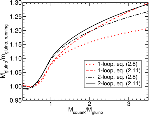
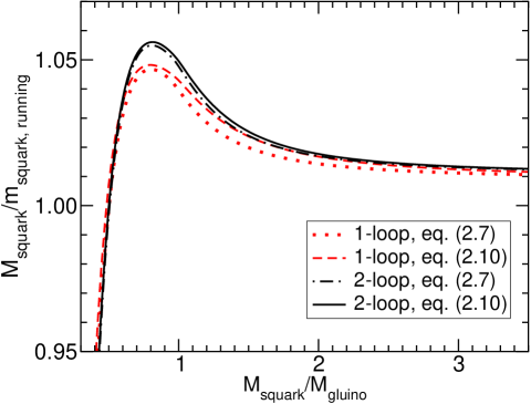
Figure 1: The ratios of the gluino and squark pole masses to the running masses, $M_{\tilde{g}}/m_{\tilde{g}}(M_{\tilde{g}})$ in the left panel and $M_{\tilde{Q}}/m_{\tilde{Q}}(M_{\tilde{Q}})$ in the right panel, as functions of the ratio of the common squark pole mass to the gluino pole mass, $M_{\tilde{Q}}/M_{\tilde{g}}$. The different lines correspond to the two-loop results of eqs. (2.8) and (2.8) and the one-loop truncations of the same formulas. For simplicity, here all squarks are taken to be degenerate and unmixed, and quark masses and electroweak effects are neglected. The renormalization scale use for the computation is $Q=M_{\tilde{g}}$ for the left panel and $Q=M_{\tilde{Q}}$ in the right panel, and the SUSYQCD coupling is fixed to $\alpha_{S}(M_{\tilde{g}})=0.095$ in both cases.

The two-loop computations of eqs. (2.8) and (2.11) for the pole mass agree to better than 1% for $M_{\tilde{Q}}/M_{\tilde{g}}<1.55$, but the disagreement increases for larger values of that ratio, and reaches 2.7% when $M_{\tilde{Q}}/M_{\tilde{g}}=3.5$. It is in just this regime that the three-loop contributions to the gluino pole mass found above should be reliable and important; I will return to this below.

In the right panel of Figure 1, the same comparison is done for the ratio of the real part of the squark pole mass to the running mass. Here, the different two-loop computations are in extremely close agreement over the entire range. Furthermore, the overall magnitude of the radiative corrections is much smaller than for the gluino. I conclude that purely theoretical uncertainties for squark masses are probably under control at a level of much better than 1 per cent. (The steep “cliff” at the left side of the graph reflects the fact that a much heavier gluino makes a large negative radiative contribution to the squark pole squared mass.)

I expect that the solid lines in Figure 1, reflecting the calculations of eqs. (2.10) and (2.11), are more reliable than those of eqs. (2.7) and (2.8). As discussed above, one reason for this expectation is the fact that the former equations do a much better job of approximating the decay widths (the imaginary parts of the pole mass) in the near-threshold region. This is illustrated in Figure 2.

 

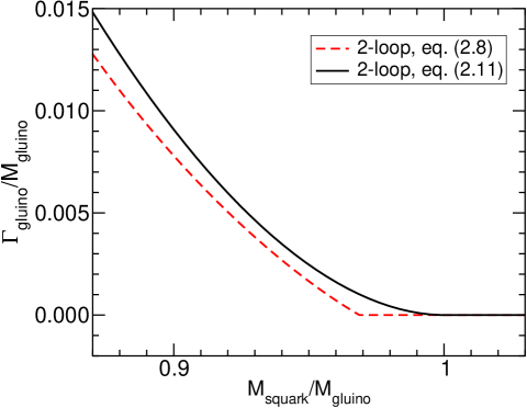
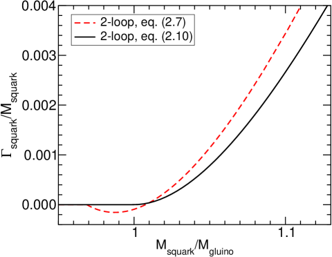
Figure 2: The gluino and squark widths as extracted from the complex pole masses, $\Gamma_{\tilde{g}}/M_{\tilde{g}}$ in the left panel and $\Gamma_{\tilde{Q}}/M_{\tilde{Q}}$ in the right panel, as functions of the ratio of the squark pole mass to the gluino pole mass, in the near-threshold region of parameter space. The different lines correspond to different two-loop approximations, as defined in the text. The widths as computed using eqs. (2.10), (2.11) agree exactly with the direct next-to-leading order width calculation of ref. Beenakker:1996dw , while the widths as computed using eqs. (2.7), (2.8) fail to agree with the decay kinematics dictated by the physical masses near threshold.

First, the gluino width $\Gamma_{\tilde{g}}$ as calculated from the pole mass using eq. (2.8) actually vanishes for all $M_{\tilde{Q}}>0.969M_{\tilde{g}}$, rather than for $M_{\tilde{Q}}\geq M_{\tilde{g}}$ as dictated by kinematics. The reason for this failure is that the width in the pole mass derives from the imaginary parts of loop integrals which, in that approximation, depend on running masses in the propagators instead of physical masses. The approximation of eq. (2.11) does not have this problem, and exactly reproduces the direct next-to-leading order width calculation of ref. Beenakker:1996dw .

A similar situation holds for the squark width, as shown in the right panel of Figure 2. In fact, the calculation of eq. (2.7) gives slightly negative (and therefore unphysical) values for the width in a narrow range on either side of the physical threshold. This is because the two-loop pole mass contribution to the width overcompensates for the one-loop contribution, which is strictly positive for all $M_{\tilde{Q}}\geq 0.969M_{\tilde{g}}$. Again, the two-loop calculation of eq. (2.10) gets the kinematics correct, and precisely reproduces the next-to-leading order calculation of ref. Beenakker:1996dw .

I next turn to the effect of the partial three-loop contributions, derived in section III, on the gluino pole mass. This is shown in Figure 3.

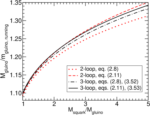
Figure 3: The ratio of the gluino pole mass to the running mass, $M_{\tilde{g}}/m_{\tilde{g}}(M_{\tilde{g}})$, as a function of the ratio of the squark pole masses to the gluino pole mass, $M_{\tilde{Q}}/M_{\tilde{g}}$, as in Figure 1. The different lines correspond to different two-loop and partial three-loop approximations, as defined in the text.

Strictly speaking, the three-loop calculations given here are only valid in the formal limit $M_{\tilde{Q}}^{2}\gg M_{\tilde{g}}^{2}$, but in any case the applied correction is small for squark masses just above the gluino mass, so I have taken the liberty of showing the entire range $M_{\tilde{Q}}>M_{\tilde{g}}$. The two three-loop approximations are much closer to each other than the corresponding two-loop approximations, just as one might have hoped. They differ by less than 1% even for $M_{\tilde{Q}}/M_{\tilde{g}}=5.$ It is also noteworthy that both three-loop results are closer to the two-loop approximation of eq. (2.11) than they are to eq. (2.8), providing some circumstantial evidence for the superiority of eq. (2.11).

Finally, consider the renormalization group scale dependence of the calculated relationship between the pole mass and the running mass of the gluino. Numerical results are shown in Figure 4, for three ratios $M_{\tilde{g}}/M_{\tilde{Q}}=0.9$, $1.5$, and $3$.

 

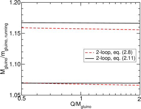
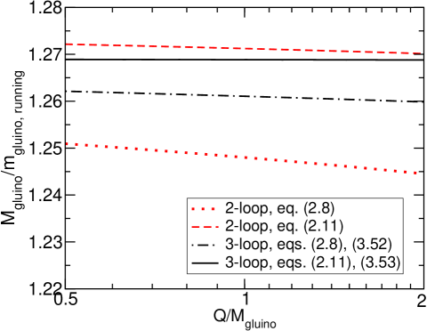
Figure 4: Renormalization-group scale ($Q$) dependence of the ratio of the gluino pole mass to the running mass, $M_{\tilde{g}}/m_{\tilde{g}}(M_{\tilde{g}})$. The left panel shows the two-loop approximations of eqs. (2.8) and (2.11), for $M_{\tilde{g}}/M_{\tilde{Q}}=0.9$ (lower pair of lines) and $M_{\tilde{g}}/M_{\tilde{Q}}=1.5$ (upper pair of lines). The right panel shows the same information, and also the three-loop approximate contributions of eqs. (3.52) and (3.53), for $M_{\tilde{g}}/M_{\tilde{Q}}=3$.

In each case, the ratio of the pole mass $M_{\tilde{g}}$ to the running mass evaluated at the pole mass, $m_{\tilde{g}}(M_{\tilde{g}})$ is computed for a fixed model in terms of the renormalization scale $Q$ at which the calculation of the pole mass is performed. The renormalization group equations (3.21)-(3.27) are used to run the running parameters between different values of $Q$. Comparing the two-loop results, the approximation of eq. (2.11) is slightly more stable than that found using eq. (2.8), although both are quite acceptably scale-invariant for $M_{\tilde{g}}/M_{\tilde{Q}}=0.9$ and $1.5$. In the case of $M_{\tilde{g}}/M_{\tilde{Q}}=3$, shown in the right panel, I also include the three-loop contributions of eqs. (3.52) and (3.53). They exhibit a still further improved scale dependence; this is encouraging but cannot be counted as a surprising triumph, since the explicit $Q$ dependence of the three-loop contribution to the pole mass came from nothing other than the three-loop beta functions.

V Conclusion

In this paper, I have argued in favor of a reformulation of the two-loop approximation between pole and running squared masses. As an improvement over eq. (2.5), equation (2.6) has general applicability. It was applied here to the specific case of gluinos and squarks in the SUSYQCD sector of the MSSM in eqs. (2.10) and (2.11). I also used the method of effective field theory to obtain a partial three-loop approximation to the gluino pole mass, when squarks are heavier. The agreement between the three-loop gluino pole mass results and the two-loop approximation of eq. (2.11) provides evidence that the method of expanding running masses about the real part of pole masses in the loop corrections provides better accuracy. Another piece of evidence in favor of this conjecture is the agreement of the imaginary part of the pole mass with a direct calculation of the width. Also, the improved renormalization scale dependence is at least consistent with it. If the LHC discovers strongly interacting superpartners, then the quest to decipher the organizing principle behind supersymmetry breaking should eventually benefit from the improved results presented here, as well as similar applications to the rest of the sparticle spectrum.

Appendix: Three-loop results for gauge theories with fermions in arbitrary representations

In this Appendix, I compile the following results for a general gauge theory renormalized in the $\overline{\rm MS}$ scheme with fermions in arbitrary representations and no scalar fields:

• the three-loop beta functions for gauge couplings,

• the three-loop beta functions for fermion masses, and

• the three-loop relation between the pole and running $\overline{\rm MS}$ masses, in the limit that there is only one non-vanishing fermion mass parameter.

Each of these results has appeared before in the case of theories that are QCD-like (containing a single gauge group and a single type of fermion representation). However, there are non-trivial ambiguities in inferring the three-loop results for general theories from the published literature. The purpose here is to resolve these ambiguities for use in the main text of the present paper and for future reference.

To set notation, consider a theory with a gauge group $G$ which is the product of one or more simple or $U(1)$ gauge groups $G_{a}$, each with a distinct $\overline{\rm MS}$ gauge coupling $g_{a}$. Results will be written in terms of the combinations

$$h_{a}\equiv g_{a}^{2}/16\pi^{2}.$$ (A.1)

Suppose further that the two-component Weyl fermions of the theory transform in possibly distinct representations of the gauge group labelled by $R$. Each Dirac (Majorana) fermion consists of two (one) such Weyl fermions, so this entails no loss of generality. The quadratic Casimir invariants of the adjoint and fermion representations of each gauge group are written as $C_{a}(A)$ and $C_{a}(R)$, respectively. The normalization is such that $C_{a}(A)=N$ for $SU(N)$, and $C_{a}(R)=(N^{2}-1)/2N$ when $R$ is a fundamental representation of $SU(N)$. The Dynkin index of each representation $R$ is written as $I_{a}(R)$, in a normalization such that the fundamental representation of $SU(N)$ has index $1/2$ for a Weyl fermion. I also define the invariants:

$$S_{a} = \sum_{R}I_{a}(R),$$ (A.2)

$$S_{ab} = \sum_{R}I_{a}(R)C_{b}(R),$$ (A.3)

$$S_{abc} = \sum_{R}I_{a}(R)C_{b}(R)C_{c}(R).$$ (A.4)

Note that a Dirac fermion contributes twice to each of these sums. For example, a Dirac fermion in a fundamental representation of $SU(N)$ will contribute 1 to $S_{a}$, and a Dirac fermion with charge $q$ under a $U(1)$ gauge group will contribute $2q^{2}$ to the corresponding $S_{a}$.

The three-loop beta function for each of the $\overline{\rm MS}$ gauge couplings is:

$$\beta_{h_{a}}\>\equiv\>Q\frac{d}{dQ}h_{a}\>=\>\beta_{h_{a}}^{(1)}+\beta_{h_{a}}^{(2)}+\beta_{h_{a}}^{(3)}+\ldots$$ (A.5)

where the terms in the loop expansion are:

$$\beta_{h_{a}}^{(1)} = h_{a}^{2}[-22C_{a}(A)+4S_{a}]/3,$$ (A.6)

$$\beta_{h_{a}}^{(2)} = h_{a}^{3}C_{a}(A)\bigl{[}-68C_{a}(A)+20S_{a}\bigr{]}/3+4h_{a}^{2}h_{b}S_{ab},$$ (A.7)

$$\beta_{h_{a}}^{(3)} = h_{a}^{4}C_{a}(A)\bigl{\{}-2857[C_{a}(A)]^{2}+1415C_{a}(A)S_{a}-79[S_{a}]^{2}\bigr{\}}/27$$ (A.8)

$$+h_{a}^{3}h_{b}8C_{a}(A)S_{ab}+h_{a}^{2}h_{b}^{2}S_{ab}\bigl{[}133C_{b}(A)-22S_{b}\bigr{]}/9-2h_{a}^{2}h_{b}h_{c}S_{abc},$$

with the indices $b$ and $c$ implicitly summed over in each term where they appear. The special case of this result for a QCD-like theory with a single gauge group component and a single type of fermion representation was given in ref. Tarasov:1980au . (The four-loop result has also been obtained in QCD-like theories, in vanRitbergen:1997va ). In that special case, the three-loop terms proportional to $h_{a}^{3}h_{b}C_{a}(A)S_{ab}$ and $h_{a}^{2}h_{b}^{2}S_{ab}C_{b}(A)$ are combined, and the term proportional to $h_{a}^{2}h_{b}^{2}S_{ab}S_{b}$ could in principle combine with a term proportional to $h_{a}^{3}h_{b}S_{ab}S_{a}$, which is actually absent. These two ambiguities have been resolved by considering the special case of the electromagnetic coupling beta function with QCD effects included; see for example eq. (54) of Chetyrkin:1997un and eqs. (9)-(10) of Erler:1998sy .

Next consider the three-loop $\overline{\rm MS}$ beta function for the mass $m$ of a fermion transforming in a representation $F$, given for a QCD-like theory in Tarasov:1982gk . Chiral symmetry guarantees that if there are several such masses, they each run independently. As far as I know, the result for a theory with different fermion representations has not been given directly in the published literature, but can be inferred by considering the results given for individual classes of diagrams in Tarasov:1982gk . The result is:

$$\beta_{m}\>\equiv\>Q\frac{d}{dQ}m\>=\>m\left[\beta_{m}^{(1)}+\beta_{m}^{(2)}+\beta_{m}^{(3)}+\ldots\right],$$ (A.9)

where the terms in the loop expansion are:

$$\beta_{m}^{(1)} = -6h_{a}C_{a}(F),$$ (A.10)

$$\beta_{m}^{(2)} = h_{a}^{2}C_{a}(F)\bigl{[}-97C_{a}(A)+10S_{a}\bigr{]}/3-3h_{a}h_{b}C_{a}(F)C_{b}(F),$$ (A.11)

$$\beta_{m}^{(3)} = h_{a}^{3}C_{a}(F)\Bigl{\{}-\frac{11413}{54}[C_{a}(A)]^{2}+\Bigl{[}\frac{556}{27}+48\zeta_{3}\Bigr{]}C_{a}(A)S_{a}+\frac{70}{27}(S_{a})^{2}\Bigr{\}}$$ (A.12)

$$+h_{a}^{2}h_{b}C_{a}(F)\Bigl{\{}\frac{129}{2}C_{a}(A)C_{b}(F)+S_{a}C_{b}(F)+[45-48\zeta_{3}]S_{ab}\Bigr{\}}-129h_{a}h_{b}h_{c}C_{a}(F)C_{b}(F)C_{c}(F).\phantom{xxx}$$

with indices $a,b,c$ summed over in terms in which they appear. The terms proportional to $C_{a}(F)S_{a}C_{b}(F)$ and $C_{a}(F)S_{ab}$ are combined in the case of quark masses in QCD, and it is this ambiguity that has been removed using the results inferred from Tarasov:1982gk . (The QCD-like case has been extended to four-loop order in fourloopbetaM .)

Finally, consider the three-loop fermion pole mass. Let the two-component fermions consist of massless fermion species with representations labelled by $r$, as well as degenerate massive fermion(s) with representation labelled by $F$ and a running mass $m(Q)$. This is only technically natural if $F$ is irreducible (as for Majorana fermions), or consists of an irreducible representation and its conjugate (as for Dirac fermions), or if $F$ consists of three or more degenerate copies of a single irreducible representation and/or its conjugate (a situation for which I know of no examples in proposed extensions of the Standard Model). Therefore, it is assumed here that all of the irreducible representations labelled by $F$ have the same Casimir invariant $C_{a}(F)$ and index $I_{a}(F)$. The invariants $S_{a}$, $S_{ab}$ previously defined are now separated into contributions from the massless and massive fermions:

$$S_{a}^{L} = \sum_{r}I_{a}(r),\qquad\qquad\!\!\!\!\!S_{a}^{H}\>=\>\sum_{F}I_{a}(F),$$ (A.13)

$$S_{ab}^{L} = \sum_{r}I_{a}(r)C_{b}(r),\qquad\!\!\!\!\!\!S_{ab}^{H}=\sum_{F}I_{a}(F)C_{b}(F).\phantom{xxxxxx}$$ (A.14)

(Again one must remember that the representations are defined for two-component fermions, so each Dirac fermion contributes twice to the appropriate sums.) Then the fermion pole mass $M$ is related to the running $\overline{\rm MS}$ mass $m$ evaluated at a renormalization scale $Q=M$ by:

$$m(M)=M\Bigl{[}1+x^{(1)}+x^{(2)}+x^{(3)}+\ldots\bigr{]},$$ (A.15)

where the loop expansion terms are:

$$x^{(1)} = -h_{a}4C_{a}(F),$$ (A.16)

$$x^{(2)} = h_{a}^{2}C_{a}(F)\bigl{\{}C_{a}(A)[-1111/24+4\pi^{2}/3-4\pi^{2}\ln 2+6\zeta_{3}]+S_{a}^{L}[71+8\pi^{2}]/12+S_{a}^{H}[143-16\pi^{2}]/12\bigr{\}}$$ (A.17)

$$+h_{a}h_{b}C_{a}(F)C_{b}(F)[8\pi^{2}\ln 2-5\pi^{2}-12\zeta_{3}+7/8],$$

$$x^{(3)} = 64h_{a}C_{a}(F)\Bigl{[}h_{b}h_{c}C_{b}(F)C_{c}(F)d^{(3)}_{1}+h_{a}h_{b}\bigl{\{}C_{a}(A)C_{b}(F)d^{(3)}_{2}+S_{ab}^{L}d^{(3)}_{4A}/2+S_{a}^{L}C_{b}(F)d^{(3)}_{4B}/2+S_{ab}^{H}d^{(3)}_{5}/2\bigr{\}}\phantom{xx}$$ (A.18)

$$\!\!\!\!\!\!\!\!\!\!\!+h_{a}^{2}\bigl{\{}[C_{a}(A)]^{2}d^{(3)}_{3}+C_{a}(A)S_{a}^{L}d^{(3)}_{6}/2+C_{a}(A)S_{a}^{H}d^{(3)}_{7}/2+S_{a}^{L}S_{a}^{H}d^{(3)}_{8}/4+\bigl{[}S_{a}^{H}\bigr{]}^{2}d^{(3)}_{9}/4+\bigl{[}S_{a}^{L}\bigr{]}^{2}d^{(3)}_{10}/4\bigr{\}}\Bigr{]},$$

with indices $a,b,c$ summed over wherever they appear. The coefficients $d_{n}^{(3)}$ were found in ref. Melnikov:2000qh for $n=1,2,3,5,6,7,8,9,10$ and will not be repeated here. The remaining coefficients $d_{4A}^{(3)}$ and $d_{4B}^{(3)}$ were combined into a single coefficient $d_{4}^{(3)}$ in that paper, since those terms are indistinguishable in the special case of a single type of fermion representation. In this paper, I need the generalized result:

$$d_{4A}^{(3)} = 827/384+\pi^{2}/16-\pi^{4}/240-11\zeta_{3}/8,$$ (A.19)

$$d_{4B}^{(3)} = \frac{85}{1152}+\frac{95}{144}\pi^{2}-\frac{11}{9}\pi^{2}\ln 2+\frac{11}{3}\zeta_{3}-\frac{11}{216}\pi^{4}$$ (A.20)

$$+\frac{2}{9}\pi^{2}\ln^{2}2+\frac{1}{9}\ln^{4}2+\frac{8}{3}{\rm Li}_{4}(1/2).$$

I obtained $d_{4A}^{(3)}$ by a direct computation of the corresponding three-loop diagrams, and then obtained $d_{4B}^{(3)}=d_{4}^{(3)}-d_{4A}^{(3)}$ using the result for $d_{4}^{(3)}$ provided in ref. Melnikov:2000qh . This was also checked independently using a slight modification of the computer code used in ref. Melnikov:2000qh , kindly provided by Kirill Melnikov.

In the application of the present paper, the effective theory with squarks decoupled consists of an $SU(3)_{c}$ gauge theory with 6 flavors of “massless” Dirac fermion quarks and 1 massive color octet Majorana gluino. Therefore, $h_{a}=\alpha_{S}/4\pi$ and the relevant group theory invariants are:

$$\!\!\!\!\!\!C_{a}(A)=C_{a}(F)=3,$$ (A.21)

$$\!\!\!\!\!\!S_{a}^{L}=6,\qquad S_{aa}^{L}=8,\qquad S_{aaa}^{L}=32/3,$$ (A.22)

$$\!\!\!\!\!\!S_{a}^{H}=3,\qquad S_{aa}^{H}=9,\qquad S_{aaa}^{H}=27,$$ (A.23)

$$\!\!\!\!\!\!S_{a}=9,\qquad S_{aa}=17,\qquad S_{aaa}=113/3.\phantom{xxx}$$ (A.24)

Acknowledgments: I am grateful to Kirill Melnikov for supplying the computer code used in ref. Melnikov:2000qh , which I used to check eqs. (A.19) and (A.20) of the present paper. I also thank Oleg Tarasov for a communication regarding ref. Tarasov:1982gk . This work was supported by the National Science Foundation under Grant No. PHY-0456635.

References

- (1) S. Dimopoulos and S. Raby, Nucl. Phys. B 192, 353 (1981); E. Witten, Nucl. Phys. B 188, 513 (1981); M. Dine, W. Fischler and M. Srednicki, Nucl. Phys. B 189, 575 (1981); S. Dimopoulos and H. Georgi, Nucl. Phys. B 193, 150 (1981); N. Sakai, Z. Phys. C 11, 153 (1981); R.K. Kaul and P. Majumdar, Nucl. Phys. B 199, 36 (1982).
- (2) For a review, see S.P. Martin, “A supersymmetry primer,” [hep-ph/9709356] (revised June 2006).
- (3) R. Tarrach, Nucl. Phys. B 183, 384 (1981).
- (4) D. Atkinson and M. P. Fry, Nucl. Phys. B 156, 301 (1979).
- (5) J.C. Breckenridge, M.J. Lavelle and T.G. Steele, Z. Phys. C 65, 155 (1995).
- (6) A.S. Kronfeld, Phys. Rev. D 58, 051501 (1998).
- (7) S. Willenbrock and G. Valencia, Phys. Lett. B 259, 373 (1991).
- (8) R.G. Stuart, Phys. Lett. B 262, 113 (1991), Phys. Lett. B 272, 353 (1991), Phys. Rev. Lett. 70, 3193 (1993).
- (9) A. Sirlin, Phys. Lett. B 267, 240 (1991), Phys. Rev. Lett. 67, 2127 (1991).
- (10) M. Passera and A. Sirlin, Phys. Rev. Lett. 77, 4146 (1996) [hep-ph/9607253], Phys. Rev. D 58, 113010 (1998) [hep-ph/9804309].
- (11) P. Gambino and P.A. Grassi, Phys. Rev. D 62, 076002 (2000), [hep-ph/9907254] P.A. Grassi, B.A. Kniehl and A. Sirlin, Phys. Rev. Lett. 86, 389 (2001), [hep-th/0005149] Phys. Rev. D 65, 085001 (2002). [hep-ph/0109228]
- (12) I.I.Y. Bigi, M.A. Shifman, N.G. Uraltsev and A.I. Vainshtein, Phys. Rev. D 50, 2234 (1994), M. Beneke and V.M. Braun, Nucl. Phys. B 426, 301 (1994).
- (13) M.C. Smith and S.S. Willenbrock, Phys. Rev. Lett. 79, 3825 (1997), A.H. Hoang, M.C. Smith, T. Stelzer and S. Willenbrock, Phys. Rev. D 59, 114014 (1999), M. Beneke, Phys. Lett. B 434, 115 (1998), M. Beneke et al., [hep-ph/0003033].
- (14) G. ’t Hooft and M. J. Veltman, Nucl. Phys. B 44, 189 (1972); W.A. Bardeen, A. J. Buras, D. W. Duke and T. Muta, Phys. Rev. D 18, 3998 (1978).
- (15) W. Siegel, Phys. Lett. B 84, 193 (1979); D.M. Capper, D.R.T. Jones and P. van Nieuwenhuizen, Nucl. Phys. B 167, 479 (1980).
- (16) I. Jack et al, Phys. Rev. D 50, 5481 (1994) [hep-ph/9407291]. The two-loop parameter redefinitions between and have been obtained in S.P. Martin, Phys. Rev. D 65, 116003 (2002) [hep-ph/0111209],
- (17) S.P. Martin and M.T. Vaughn, Phys. Lett. B 318, 331 (1993) [hep-ph/9308222].
- (18) D. Pierce and A. Papadopoulos, Phys. Rev. D 50, 565 (1994) [hep-ph/9312248]. Nucl. Phys. B 430, 278 (1994) [hep-ph/9403240].
- (19) D.M. Pierce, J.A. Bagger, K.T. Matchev and R.J. Zhang, Nucl. Phys. B 491, 3 (1997) [hep-ph/9606211].
- (20) G. Degrassi, S. Heinemeyer, W. Hollik, P. Slavich and G. Weiglein, Eur. Phys. J. C 28, 133 (2003) [hep-ph/0212020].
- (21) J.S. Lee et al, Comput. Phys. Commun. 156, 283 (2004) [hep-ph/0307377].
- (22) S.P. Martin, Phys. Rev. D 66, 096001 (2002) [hep-ph/0206136]; Phys. Rev. D 67, 095012 (2003) [hep-ph/0211366]. S.P. Martin, Phys. Rev. D 71, 016012 (2005) [hep-ph/0405022].
- (23) B.C. Allanach, A. Djouadi, J.L. Kneur, W. Porod and P. Slavich, JHEP 0409, 044 (2004) [hep-ph/0406166].
- (24) S. Heinemeyer, Int. J. Mod. Phys. A 21, 2659 (2006) [hep-ph/0407244]. S. Heinemeyer, W. Hollik, H. Rzehak and G. Weiglein, Eur. Phys. J. C 39, 465 (2005) [hep-ph/0411114]. T. Hahn, W. Hollik, S. Heinemeyer and G. Weiglein, “Precision Higgs masses with FeynHiggs 2.2,” [hep-ph/0507009].
- (25) S.P. Martin, Phys. Rev. D 71, 116004 (2005) [hep-ph/0502168].
- (26) Y. Yamada, Phys. Lett. B 623, 104 (2005) [hep-ph/0506262].
- (27) S.P. Martin, Phys. Rev. D 72, 096008 (2005) [hep-ph/0509115].
- (28) A. Bednyakov, A. Onishchenko, V. Velizhanin and O. Veretin, Eur. Phys. J. C 29, 87 (2003) [hep-ph/0210258]; A. Bednyakov and A. Sheplyakov, Phys. Lett. B 604, 91 (2004) [hep-ph/0410128]; A. Bednyakov, D. I. Kazakov and A. Sheplyakov, “On the two-loop O(alpha(s)**2) corrections to the pole mass of the t-quark in the MSSM,” [hep-ph/0507139]. See also H. Baer, J. Ferrandis, K. Melnikov and X. Tata, Phys. Rev. D 66, 074007 (2002) [hep-ph/0207126].
- (29) S.P. Martin, Phys. Rev. D 68, 075002 (2003) [hep-ph/0307101]; S.P. Martin and D.G. Robertson, “TSIL: a program for the calculation of two-loop self-energy integrals”, Comput. Phys. Commun. 174, 133 (2006), [hep-ph/0501132]. The numerical method used by this program for generic masses is similar to the one proposed earlier in ref. CCLR . The program also uses analytical results when available in special cases, including those found in refs. Tarasov:1997kx ; Mertig:1998vk ; Gray:1990yh ; Fleischer:1998dw ; Jegerlehner:2003py ; vanderBij:1983bw ; Broadhurst:1987ei ; Djouadi:1987di ; Ford:hw ; Scharf:1993ds ; Berends:1994ed ; Berends:1997vk ; Fleischer:1998nb ; Davydychev:1998si ; Fleischer:1999hp .
- (30) M. Caffo, H. Czyz, S. Laporta and E. Remiddi, Nuovo Cim. A 111, 365 (1998) [hep-th/9805118]; Acta Phys. Polon. B 29, 2627 (1998) [hep-th/9807119]; M. Caffo, H. Czyz and E. Remiddi, Nucl. Phys. B 634, 309 (2002) hep-ph/0203256; “Numerical evaluation of master integrals from differential equations,” [hep-ph/0211178], M. Caffo, H. Czyz, A. Grzelinska and E. Remiddi, Nucl. Phys. B 681, 230 (2004) [hep-ph/0312189].
- (31) O.V. Tarasov, Nucl. Phys. B 502, 455 (1997) [hep-ph/9703319].
- (32) R. Mertig and R. Scharf, Comput. Phys. Commun. 111, 265 (1998) [hep-ph/9801383].
- (33) N. Gray, D.J. Broadhurst, W. Grafe and K. Schilcher, Z. Phys. C 48, 673 (1990).
- (34) J. Fleischer, F. Jegerlehner, O.V. Tarasov and O.L. Veretin, Nucl. Phys. B 539, 671 (1999) [Erratum-ibid. B 571, 511 (2000)] [hep-ph/9803493].
- (35) F. Jegerlehner and M.Y. Kalmykov, Nucl. Phys. B 676, 365 (2004) [hep-ph/0308216].
- (36) J. van der Bij and M.J.G. Veltman, Nucl. Phys. B 231, 205 (1984).
- (37) D.J. Broadhurst, Z. Phys. C 47, 115 (1990).
- (38) A. Djouadi, Nuovo Cim. A 100, 357 (1988).
- (39) C. Ford and D.R.T. Jones, Phys. Lett. B 274, 409 (1992); C. Ford, I. Jack and D.R.T. Jones, Nucl. Phys. B 387, 373 (1992) [hep-ph/0111190].
- (40) R. Scharf and J.B. Tausk, Nucl. Phys. B 412, 523 (1994).
- (41) F.A. Berends and J.B. Tausk, Nucl. Phys. B 421, 456 (1994).
- (42) F.A. Berends, A.I. Davydychev and N.I. Ussyukina, Phys. Lett. B 426, 95 (1998) [hep-ph/9712209].
- (43) J. Fleischer, A.V. Kotikov and O.L. Veretin, Nucl. Phys. B 547, 343 (1999) [hep-ph/9808242].
- (44) A.I. Davydychev and A.G. Grozin, Phys. Rev. D 59, 054023 (1999) [hep-ph/9809589].
- (45) J. Fleischer, M.Y. Kalmykov and A.V. Kotikov, Phys. Lett. B 462, 169 (1999) [hep-ph/9905249].
- (46) W. Beenakker, R. Hopker and P.M. Zerwas, Phys. Lett. B 378, 159 (1996) [hep-ph/9602378]. Note that the appearing in eqs. (9)-(12) of this reference is the one. To convert the result to in , one can replace in those equations. The corresponding results including squark mixing are found in ref. Beenakker:1996de .
- (47) W. Beenakker, R. Hopker, T. Plehn and P.M. Zerwas, Z. Phys. C 75, 349 (1997) [hep-ph/9610313].
- (48) J.D. Wells, “Implications of supersymmetry breaking with a little hierarchy between gauginos and scalars,” [hep-ph/0306127]; Phys. Rev. D 71, 015013 (2005) [hep-ph/0411041].
- (49) N. Arkani-Hamed and S. Dimopoulos, JHEP 0506, 073 (2005) [hep-th/0405159]; G. F. Giudice and A. Romanino, Nucl. Phys. B 699, 65 (2004) [Erratum-ibid. B 706, 65 (2005)] [hep-ph/0406088],
- (50) K. Melnikov and T. v. Ritbergen, Phys. Lett. B 482, 99 (2000) [hep-ph/9912391].
- (51) O.V. Tarasov, “Anomalous Dimensions Of Quark Masses In Three Loop Approximation,” preprint JINR-P2-82-900, (1982), unpublished.
- (52) I. Jack, D.R.T. Jones and K.L. Roberts, Z. Phys. C 62, 161 (1994) [hep-ph/9310301]; Z. Phys. C 63, 151 (1994) [hep-ph/9401349]; R. Harlander, P. Kant, L. Mihaila and M. Steinhauser, “Dimensional reduction applied to QCD at three loops,” [hep-ph/0607240].
- (53) P.M. Ferreira, I. Jack and D.R.T. Jones, Phys. Lett. B 387, 80 (1996) [hep-ph/9605440]. I. Jack, D.R.T. Jones and C.G. North, Phys. Lett. B 386, 138 (1996) [hep-ph/9606323].
- (54) S.P. Martin and M.T. Vaughn, Phys. Lett. B 318, 331 (1993) [hep-ph/9308222];
- (55) I. Jack and D.R.T. Jones, Phys. Lett. B 415, 383 (1997) [hep-ph/9709364].
- (56) S.P. Martin and M. T. Vaughn, Phys. Rev. D 50, 2282 (1994) [hep-ph/9311340]. Y. Yamada, Phys. Rev. D 50, 3537 (1994) [hep-ph/9401241]. I. Jack and D.R.T. Jones, Phys. Lett. B 333, 372 (1994) [hep-ph/9405233].
- (57) R. Harlander, L. Mihaila and M. Steinhauser, Phys. Rev. D 72, 095009 (2005) [hep-ph/0509048].
- (58) O.V. Tarasov, A.A. Vladimirov and A.Y. Zharkov, Phys. Lett. B 93, 429 (1980).
- (59) T. van Ritbergen, J.A.M. Vermaseren and S.A. Larin, Phys. Lett. B 400, 379 (1997) [hep-ph/9701390].
- (60) K.G. Chetyrkin, B.A. Kniehl and M. Steinhauser, Nucl. Phys. B 510, 61 (1998) [hep-ph/9708255].
- (61) J. Erler, Phys. Rev. D 59, 054008 (1999) [hep-ph/9803453].
- (62) K.G. Chetyrkin, Phys. Lett. B 404, 161 (1997) [hep-ph/9703278]; J.A.M. Vermaseren, S.A. Larin and T. van Ritbergen, Phys. Lett. B 405, 327 (1997) [hep-ph/9703284].