Bottomonium Production in the Regge Limit of QCD

Abstract

We study bottomonium hadroproduction in proton-antiproton collisions at the Fermilab Tevatron in the framework of the quasi-multi-Regge kinematics approach and the factorization formalism of non-relativistic QCD at leading order in the strong-coupling constant $\alpha_{s}$ and the relative velocity $v$ of the bound quarks. The transverse-momentum distributions of prompt $\Upsilon(nS)$-meson production measured at the Tevatron are fitted to obtain the non-perturbative long-distance matrix elements for different choices of un-integrated gluon distribution functions of the proton.

I Introduction

Bottomonium production at high energies has provided a useful laboratory for testing the high-energy limit of quantum chromodynamics (QCD) as well as the interplay of perturbative and non-perturbative phenomena in QCD. The factorization formalism of non-relativistic QCD (NRQCD) NRQCD is a rigorous theoretical framework for the description of heavy-quarkonium production and decay. The factorization hypothesis of NRQCD assumes the separation of the effects of long and short distances in heavy-quarkonium production. NRQCD is organized as a perturbative expansion in two small parameters, the strong-coupling constant $\alpha_{s}$ and the relative velocity $v$ of the heavy quarks.

The phenomenology of strong interactions at high energies exhibits a dominant role of gluon interactions in quarkonium production. In the conventional parton model PartonModel , the initial-state gluon dynamics is controlled by the Dokshitzer-Gribov-Lipatov-Altarelli-Parisi (DGLAP) evolution equation DGLAP . In this approach, it is assumed that $S>\mu^{2}\gg\Lambda_{\rm QCD}^{2}$, where $\sqrt{S}$ is the invariant collision energy, $\mu$ is the typical energy scale of the hard interaction, and $\Lambda_{\rm QCD}$ is the asymptotic scale parameter of QCD. In this way, the DGLAP evolution equation takes into account only one big logarithm, namely $\ln(\mu/\Lambda_{\rm QCD})$. In fact, the collinear-partron approximation is used, and the transverse momenta of the incoming gluons are neglected.

In the high-energy limit, the contribution from the partonic subprocesses involving $t$-channel gluon exchanges to the total cross section can become dominant. The summation of the large logarithms $\ln(\sqrt{S}/\mu)$ in the evolution equation can then be more important than the one of the $\ln(\mu/\Lambda_{\rm QCD})$ terms. In this case, the non-collinear gluon dynamics is described by the Balitsky-Fadin-Kuraev-Lipatov (BFKL) evolution equation BFKL . In the region under consideration, the transverse momenta ($k_{T}$) of the incoming gluons and their off-shell properties can no longer be neglected, and we deal with reggeized $t$-channel gluons. The theoretical frameworks for this kind of high-energy phenomenology are the $k_{T}$-factorization approach KTGribov ; KTCollins and the quasi-multi-Regge kinematics (QMRK) approach KTLipatovFadin ; KTAntonov , which is based on effective quantum field theory implemented with the non-abelian gauge-invariant action, as suggested a few years ago KTLipatov . Our previous analysis of charmonium production at high-energy colliders using the high-energy factorization scheme KniehlSaleevVasin ; PRD2003 has shown the equivalence of the $k_{T}$-factorization and the QMRK approaches at leading order (LO) in $\alpha_{s}$. However, the $k_{T}$-factorization approach has well-known principal difficulties smallx at next-to-leading order (NLO). By contrast, the QMRK approach offers a conceptual solution of the NLO problems Ostrovsky . In our LO applications, the QMRK approach yields similar formulas as the $k_{T}$-factoriztion approach, so that we can essentially continue using our previous results KniehlSaleevVasin ; PRD2003 obtained in the $k_{T}$-factorization formalism using the Collins-Ellis prescription KTCollins .

This paper is organized as follows. In Sec. II, the QMRK approach is briefly reviewed. In Sec. III, we explain how the analytic results of Refs. KniehlSaleevVasin ; PRD2003 relevant for our analysis may be converted to the QMRK framework. In Sec. IV, we perform fits to the transverse-momentum ($p_{T}=|{\bf p}_{T}|$) distributions of inclusive bottomonium production measured at the Fermilab Tevatron to obtain numerical values for the non-perturbative matrix elements (NMEs) of the NRQCD factorization formalism. In Sec. V, we summarize our results.

II QMRK approach

In the phenomenology of strong interactions at high energies, it is necessary to describe the QCD evolution of the gluon distribution functions of the colliding particles starting from some scale $\mu_{0}$, which controls a non-perturbative regime, to the typical scale $\mu$ of the hard-scattering processes, which is typically of the order of the transverse mass $M_{T}=\sqrt{M^{2}+|{\bf p}_{T}|^{2}}$ of the produced particle (or hadron jet) with (invariant) mass $M$ and transverse two-momentum ${\bf p}_{T}$. In the region of very high energies, in the so-called Regge limit, the typical ratio $x=\mu/\sqrt{S}$ becomes very small, $x\ll 1$. This leads to large logarithmic contributions of the type $[\alpha_{s}\ln(1/x)]^{n}$ in the resummation procedure, which is described by the BFKL evolution equation BFKL for an un-integrated gluon distribution function $\Phi(x,|{\bf q}_{T}|^{2},\mu^{2})$, where ${\bf q}_{T}$ is the transverse two-momentum of the gluon with respect to the flight direction of the incoming hadron from which it stems. Accordingly, in the QMRK approach KTLipatovFadin , the initial-state $t$-channel gluons are considered as reggeons (or reggeized gluons). They carry finite transverse two-momenta ${\bf q}_{T}$ with respect to the hadron beam from which they stem and are off mass shell.

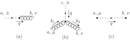
Figure 1: Feynman diagrams pertinent to the (a) PR vertex, (b) PPR vertex, and (c) reggeized-gluon propagator given in Eqs. (1), (3), and (4), respectively.

Reggeized gluons interact with quarks and Yang-Mills gluons in a specific way. Recently, in Ref. KTAntonov , the Feynman rules for the effective theory based on the non-abelian gauge-invariant action KTLipatov were derived for the induced and some important effective vertices. The induced vertex for the transition from a reggeized gluon to a Yang-Mills gluon $R^{\pm}\to g$ (PR vertex) shown in Fig. 1(a) has the form:

$$\Gamma_{ab}^{\pm\nu}(q)=i\delta^{ab}q^{2}(n^{\pm})^{\nu},$$ (1)

where $(n^{+})^{\nu}=P_{1}^{\nu}/E_{1}$, $(n^{-})^{\nu}=P_{2}^{\nu}/E_{2}$, $P_{1,2}^{\nu}$ are the four-momenta of the colliding protons, and $E_{1,2}$ are their energies in the center-of-mass frame. We have $(n^{\pm})^{2}=0$, $n^{+}\cdot n^{-}=2$, and $S=(P_{1}+P_{2})^{2}=4E_{1}E_{2}$. For any four-momentum $k^{\mu}$, we define $k^{\pm}=k\cdot n^{\pm}$. It is easy to see that the four-momenta of the reggeized gluons can be represented as

$$q_{1}^{\mu} = q_{1T}^{\mu}+\frac{q_{1}^{-}}{2}(n^{+})^{\mu},$$

$$q_{2}^{\mu} = q_{2T}^{\mu}+\frac{q_{2}^{+}}{2}(n^{-})^{\mu},$$

$$q_{1}^{+} = q_{2}^{-}=0.$$ (2)

The induced interaction vertex of one reggeized gluon with two Yang-Mills gluons (PPR vertex) depicted in Fig. 1(b) reads

$$\Gamma^{\mu\pm\nu}_{acb}(k_{1},q,k_{2})=-g_{s}f^{abc}\frac{q^{2}}{k_{1}^{\pm}}(n^{\pm})^{\mu}(n^{\pm})^{\nu},$$ (3)

where $g_{s}=\sqrt{4\pi\alpha_{s}}$ is the gauge coupling of QCD. The reggeized-gluon propagator displayed in Fig. 1(c) is given by

$$D^{\mu\nu}_{ab}(q)=-i\delta^{ab}\frac{1}{2q^{2}}\left[(n^{+})^{\mu}(n^{-})^{\nu}+(n^{+})^{\nu}(n^{-})^{\mu}\right].$$ (4)

The Lagrangian of the effective theory KTLipatov also contains the standard gluon-gluon and quark-gluon interactions for Yang-Mills gluons.

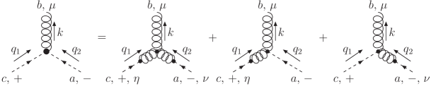
Figure 2: Feynman diagrams pertinent to the effective PRR vertex given in Eq. (5).

Using the Feynman rules for the induced vertices (1) and (3) and the ordinary vertices, one can construct effective vertices, which obey Bose and gauge symmetries. For example, the effective three-vertex that describes the production of a single Yang-Mills gluon with four-momentum $k^{\mu}=q_{1}^{\mu}+q_{2}^{\mu}$ and color index $b$ by two-reggeon annihilation $R^{+}+R^{-}\to g$ (PRR vertex) shown in Fig. 2 reads

$$\Gamma^{+\mu-}_{cba}(q_{1},k,q_{2}) = V^{\rho\sigma\mu}_{cab}(-q_{1},-q_{2},k)(n^{+})_{\rho}(n^{-})_{\sigma}+\Gamma^{\rho-\mu}_{cab}(q_{1},q_{2},k)(n^{+})_{\rho}+\Gamma^{\sigma+\mu}_{acb}(q_{2},q_{1},k)(n^{-})_{\sigma}$$ (5)

$$= 2g_{s}f^{cba}\left[(n^{-})^{\mu}\left(q_{2}^{+}+\frac{q_{2}^{2}}{q_{1}^{-}}\right)-(n^{+})^{\mu}\left(q_{1}^{-}+\frac{q_{1}^{2}}{q_{2}^{+}}\right)+(q_{1}-q_{2})^{\mu}\right],$$

where

$$V^{\lambda\mu\nu}_{abc}(k_{1},k_{2},k_{3})=-g_{s}f^{abc}\left[(k_{1}-k_{2})^{\nu}g^{\lambda\mu}+(k_{2}-k_{3})^{\lambda}g^{\mu\nu}+(k_{3}-k_{1})^{\mu}g^{\nu\lambda}\right]$$ (6)

is the Yang-Mills three-gluon vertex, with all four-momenta taken to be outgoing, and we exploited the following relation

$$\delta^{ab}(n^{\pm})^{\mu}=\Gamma^{\pm\nu}_{ac}(q)\left(-i\delta^{cb}\frac{g^{\mu\nu}}{q^{2}}\right).$$ (7)

The gauge invariance of the effective theory KTLipatov leads to the following condition for amplitudes in the QMRK:

$$\lim_{|{\bf q}_{1T}|,|{\bf q}_{1T}|\to 0}\overline{|{\cal A}(R+R\to{\cal H}+X)|^{2}}=0.$$ (8)

In the QMRK approach, the hadronic cross section of quarkonium (${\cal H}$) production through the process

$$p+\bar{p}\to{\cal H}+X$$ (9)

and the partonic cross section of the two-reggeon fusion subprocess

$$R+R\to{\cal H}+X$$ (10)

are related as

$$d\sigma(p+\bar{p}\to{\cal H}+X) = \int\frac{dx_{1}}{x_{1}}\int\frac{d^{2}{\bf q}_{1T}}{\pi}\Phi\left(x_{1},|{\bf q}_{1T}|^{2},\mu^{2}\right)\int\frac{dx_{2}}{x_{2}}\int\frac{d^{2}{\bf q}_{2T}}{\pi}$$ (11)

$${}\times\Phi\left(x_{2},|{\bf q}_{2T}|^{2},\mu^{2}\right)d\hat{\sigma}(R+R\to{\cal H}+X).$$

where $\Phi\left(x,|{\bf q}_{T}|^{2},\mu^{2}\right)$ is the un-integrated gluon distribution function in the proton, $x_{1}=q_{1}^{-}/(2E_{1})$ and $x_{2}=q_{2}^{+}/(2E_{2})$ are the fractions of the proton momenta passed on to the reggeized gluons, and the factorization scale $\mu$ is chosen to be of order $M_{T}$. The collinear and un-integrated gluon distribution functions are formally related as

$$xG(x,\mu^{2})=\int_{0}^{\mu^{2}}d|{\bf q}_{T}|^{2}\Phi\left(x,|{\bf q}_{T}|^{2},\mu^{2}\right),$$ (12)

so that, for ${\bf q}_{1T}={\bf q}_{2T}={\bf 0}$, we recover the conventional factorization formula of the collinear parton model,

$$d\sigma(p+\bar{p}\to{\cal H}+\!X)=\int{dx_{1}}G(x_{1},\mu^{2})\int{dx_{2}}G(x_{2},\mu^{2})d\hat{\sigma}(g+g\to{\cal H}+X).$$ (13)

The partonic cross section or process (10) may be evaluated as

$$d\hat{\sigma}(R+R\to{\cal H}+X)=\frac{{\cal N}}{2x_{1}x_{2}S}\overline{|{\cal A}(R+R\to{\cal H}+X)|^{2}}d\Phi,$$ (14)

where $2x_{1}x_{2}S$ is the flux factor of the incoming particles, ${\cal A}(R+R\to{\cal H}+X)$ is the production amplitude, the overbar indicates average (summation) over initial-state (final-state) spins and colors, $d\Phi$ is the phase space volume of the outgoing particles, and

$${\cal N}=\frac{(x_{1}x_{2}S)^{2}}{16|{\bf q}_{1T}|^{2}|{\bf q}_{2T}|^{2}}$$ (15)

is a normalization factor that ensures the correct transition to the collinear-parton limit. This convention implies that the partonic cross section in the QMRK approach is normalized approximately to the cross section for on-shell gluons when ${\bf q}_{1T}={\bf q}_{2T}={\bf 0}$.

In our numerical calculations, we use the un-integrated gluon distribution functions by Blümlein (JB) JB , by Jung and Salam (JS) JS , and by Kimber, Martin, and Ryskin (KMR) KMR . A direct comparison between different un-integrated gluon distributions as functions of $x$, $|{\bf k}_{T}|^{2}$, and $\mu^{2}$ may be found in Ref. PLB2002 . Note that the JB version is based on the BFKL evolution equation BFKL . On the contrary, the JS and KMR versions were obtained using the more complicated Catani-Ciafaloni-Fiorani-Marchesini (CCFM) evolution equation CCFM , which takes into account both large logarithms of the types $\ln(1/x)$ and $\ln(\mu/\Lambda_{\rm QCD})$.

III Relation between QMRK and $k_{T}$-factorization approaches

In this section, we obtain the squared amplitudes for inclusive quarkonium production via the fusion of two reggeized gluons in the framework of QMRK KTAntonov and NRQCD NRQCD . We work at LO in $\alpha_{s}$ and $v$ and consider the following partonic subprocesses KniehlSaleevVasin :

$$R+R \to {\cal H}\left[{{}^{3}P}_{J}^{(1)},{{}^{3}S}_{1}^{(8)},{{}^{1}S}_{0}^{(8)},{{}^{3}P}_{J}^{(8)}\right],$$ (16)

$$R+R \to {\cal H}\left[{{}^{3}S}_{1}^{(1)}\right]+g.$$ (17)

This formalism also allows for a consistent treatment at NLO, which is, however, beyond the scope of this paper and needs a separate investigation.

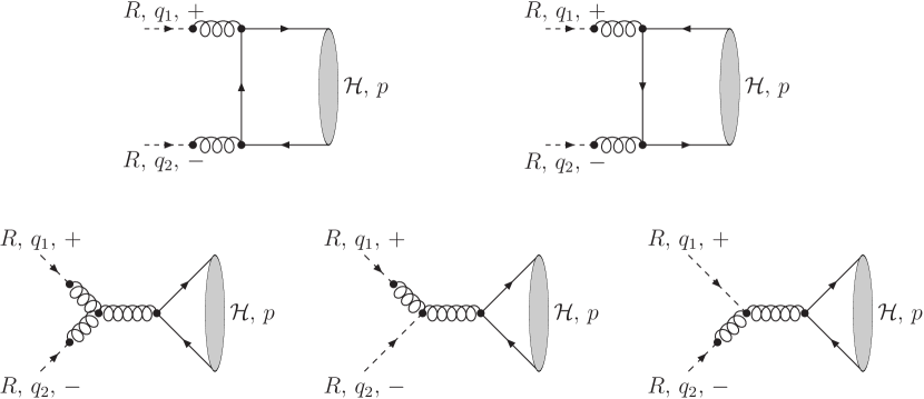
Figure 3: Feynman diagrams pertinent to processes (16).

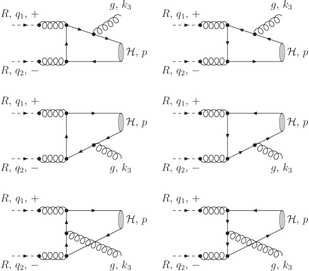
Figure 4: Feynman diagrams pertinent to process (17).

According to the prescription of Ref. KTAntonov , the amplitudes of processes (16) may be obtained from the five Feynman diagrams depicted in Fig. 3. Of course, the last three Feynman diagrams in Fig. 3 can be combined through the effective PRR vertex. The Feynman diagrams pertinent to process (17) are shown in Fig. 4.

The LO results for the squared amplitudes of subprocesses (16) and (17) that we find by using the Feynman rules of Ref. KTAntonov coincide with those we obtained in Ref. KniehlSaleevVasin in the $k_{T}$-factorization approach. The general relation between the squared amplitudes in both approaches is

$${\cal N}\overline{|{\cal A}(R+R\to{\cal H}+X)|^{2}}=\overline{|{\cal A}^{\rm KT}(R+R\to{\cal H}+X)|^{2}}.$$ (18)

The formulas for the $2\to 1$ subprocesses (16) are listed in Eq. (27) of Ref. KniehlSaleevVasin . In the case of the $2\to 2$ subprocess (17), our analytic results were not included in the journal publication of Ref. KniehlSaleevVasin for lack of space. However, they are given in Eq. (38) of the preprint version of Ref. KniehlSaleevVasin and may be obtained in FORTRAN or Mathematica format by electronic mail upon request from the authors.

The differential hadronic cross section of process (11) may then be evaluated from the squared matrix elements of processes (16) and (17) as indicated in Eqs. (46) and (48) of Ref. KniehlSaleevVasin .

IV Bottomonium production at the Tevatron

The CDF Collaboration at the Tevatron measured the $p_{T}$ distributions of $\Upsilon(1S)$, $\Upsilon(2S)$, and $\Upsilon(3S)$ mesons in the central region of rapidity ($y$), $|y|<0.4$, at $\sqrt{S}=1.8$ TeV (run I) CDFBottomI and that of the $\Upsilon(1S)$ meson in the rapidity regions $|y|<0.6$, $0.6<|y|<1.2$, and $1.2<|y|<1.8$ at $\sqrt{S}=1.96$ TeV (run II) CDFBottomII . In both cases, the $S$-wave bottomonia were produced promptly, i.e., directly or through non-forbidden decays of higher-lying $S$- and $P$-wave bottomonium states, including cascade transitions such as $\Upsilon(3S)\to\chi_{b1}(2P)\to\Upsilon(1S)$.

As is well known, the cross section of bottomonium production measured at the Tevatron at large values of $p_{T}$ is more than one order of magnitude larger than the prediction of the color-singlet model (CSM) CSM implemented in the collinear parton model QWG . Switching from the CSM to the NRQCD factorization formalism NRQCD within the collinear parton model BFL somewhat ameliorates the situation in the large-$p_{T}$ region, at $p_{T}\gtrsim 10$ GeV, but still does not lead to agreement at all values of $p_{T}$. On the other hand, the shape of the $p_{T}$ distribution can be described in the color evaporation model CEM improved by the resummation of the large logarithmic contributions from soft-gluon radiation at all orders in $\alpha_{s}$ in the region of $p_{T}<M$ Berger . However, the overall normalization of the cross section can not be predicted in this approach CEM ; Berger .

In contrast to previous analyses in the collinear parton model, we perform a joint fit to the CDF data from run I CDFBottomI and run II CDFBottomII for all $p_{T}$ values, including the small-$p_{T}$ region, to extract the color-octet NMEs of the $\Upsilon(nS)$ and $\chi_{bJ}(nP)$ mesons using three different un-integrated gluon distribution functions. Our calculations are based on exact analytical expressions for the relevant squared amplitudes, obtained in the QMRK approach as explained in Sec. III.

For the reader’s convenience, we list in Table 1 the inclusive branching fractions of the feed-down decays of the various bottomonium states, which can be gleaned from Ref. PDG2004 . Theses values supersede those presented in Ref. BFL . Since the $\Upsilon(nS)$ mesons are identified in Refs. CDFBottomI ; CDFBottomII through their decays to $\mu^{+}\mu^{-}$ pairs, we have to include the corresponding branching fractions, which we also adopt from Ref. PDG2004 , $B(\Upsilon(1S)\to\mu^{+}+\mu^{-})=0.0248$, $B(\Upsilon(2S)\to\mu^{+}+\mu^{-})=0.0131$, and $B(\Upsilon(3S)\to\mu^{+}+\mu^{-})=0.0181$. We take the pole mass of the bottom quark to be $m_{b}=4.77$ GeV.

We now present and discuss our numerical results. In Table 2, we list our fit results for the relevant color-octet NMEs for three different choices of un-integrated gluon distribution function, namely JB JB , JS JS , and KMR KMR . The relevant color-singlet NMEs are not fitted. The color-singlet NMEs of the $\Upsilon(nS)$ mesons are determined from the measured partial decay widths of $\Upsilon(nS)\to l^{+}+l^{-}$ using the vacuum saturation approximation and heavy-quark spin symmetry in the NRQCD factorization formulas and including NLO QCD radiative corrections QCDCorrections . The partial decay widths of $\chi_{b0}(nP)\to 2\gamma$, from which the color-singlet NMEs of the $\chi_{bJ}(nP)$ mesons could be extracted, are yet unknown. However, these NMEs can be estimated using the wave functions evaluated at the origin from potential models QPM , as was done in Ref. BFL . We adopt the color-singlet NMEs of the $\chi_{b0}(nP)$ mesons from Ref. BFL .

We first study the relative importance of the various color-octet $b\bar{b}$ Fock states in direct $\Upsilon(nS)$ hadroproduction. Previous fits to CDF data CDFBottomI were constrained to the large-$p_{T}$ region, $p_{T}\gtrsim 8$ GeV, and could not separate the contributions proportional to $\langle{\cal O}^{\Upsilon(nS)}[^{1}S_{0}^{(8)}]\rangle$ and $\langle{\cal O}^{\Upsilon(nS)}[^{3}P_{0}^{(8)}]\rangle$. Instead, they determined the linear combination

$$M_{r}^{\Upsilon(nS)}=\langle{\cal O}^{\Upsilon(nS)}\left[{}^{1}S_{0}^{(8)}\right]\rangle+\frac{r}{m_{b}^{2}}\langle{\cal O}^{\Upsilon(nS)}\left[{}^{3}P_{0}^{(8)}\right]\rangle,$$ (19)

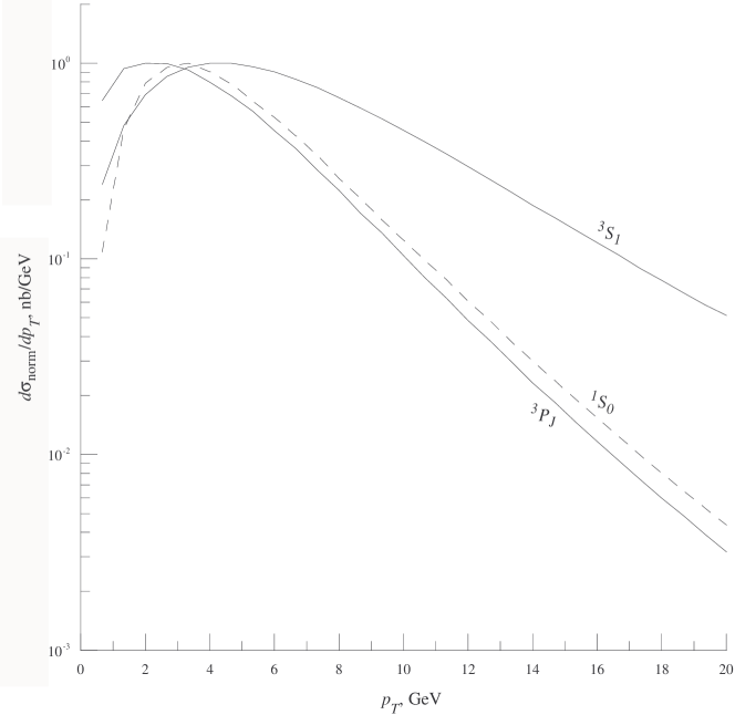
Figure 5: Contributions to the $p_{T}$ distribution of direct $\Upsilon(1S)$ hadroproduction in $p\bar{p}$ scattering with $\sqrt{S}=1.8$ TeV and $|y|<0.4$ from the relevant color-octet states. All distributions are normalized to unity at their peaks.

for the value of $r$ that minimized the error on $M_{r}^{\Upsilon(nS)}$. By contrast, the QMRK approach allows us to cover also the small-$p_{T}$ region and thus to fit $\langle{\cal O}^{\Upsilon(nS)}[^{1}S_{0}^{(8)}]\rangle$ and $\langle{\cal O}^{\Upsilon(nS)}[^{3}P_{0}^{(8)}]\rangle$ separately, thanks to the different $p_{T}$ dependences of the respective contributions for $p_{T}\lesssim 8$ GeV. This feature is nicely illustrated for direct $\Upsilon(1S)$ hadroproduction in Fig. 5, where the shapes of the contributions proportional to $\langle{\cal O}^{\Upsilon(1S)}[^{3}S_{1}^{(8)}]\rangle$, $\langle{\cal O}^{\Upsilon(1S)}[^{1}S_{0}^{(8)}]\rangle$, and $\langle{\cal O}^{\Upsilon(1S)}[^{3}P_{0}^{(8)}]\rangle$ are compared. Notice that the peak positions significantly differ, by up to 2 GeV. Apparently, this suffices to disentangle the contributions previously combined by Eq. (19).

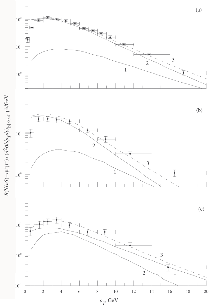
Figure 6: $p_{T}$ distributions of prompt (a) $\Upsilon(1S)$, (b) $\Upsilon(2S)$, and (c) $\Upsilon(3S)$ hadroproduction in $p\overline{p}$ scattering with $\sqrt{S}=1.8$ TeV and $|y|<0.4$ including the respective decay branching fractions $B(\Upsilon(nS)\to\mu^{+}+\mu^{-})$. The color-octet (curve 1) and color-singlet (curve 2) contributions, evaluated with the JB JB un-integrated gluon distribution function, and their sum (curve 3) are compared with the CDF data from run I CDFBottomI .

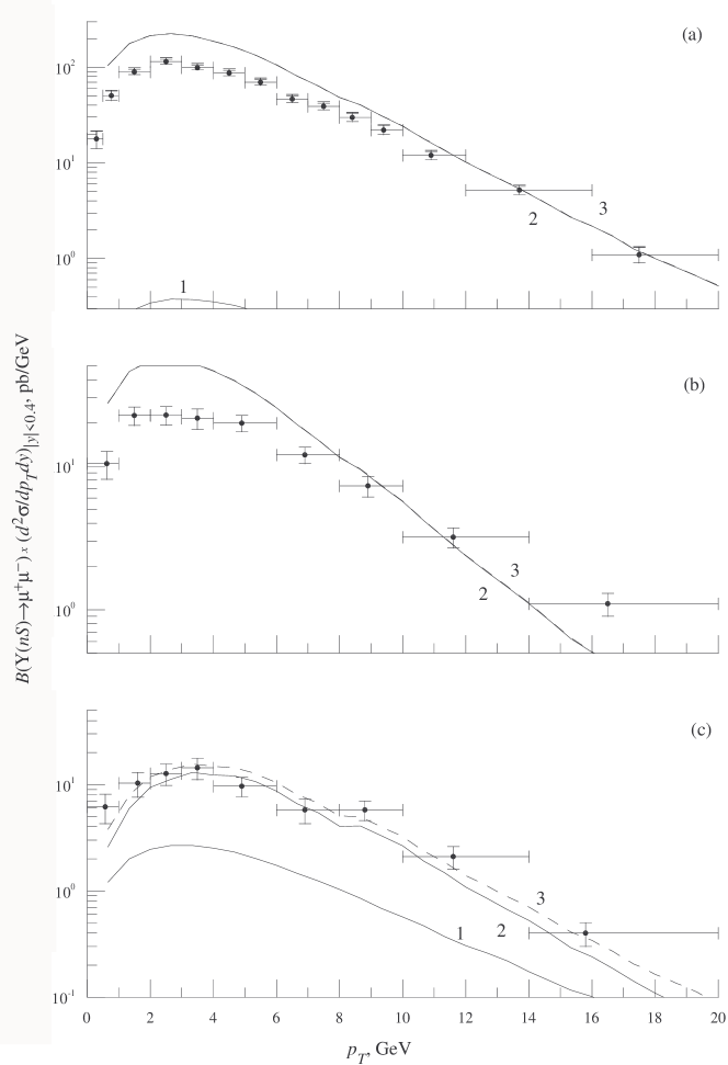
Figure 7: Same as in Fig. 6, but for the JS JS un-integrated gluon distribution function.

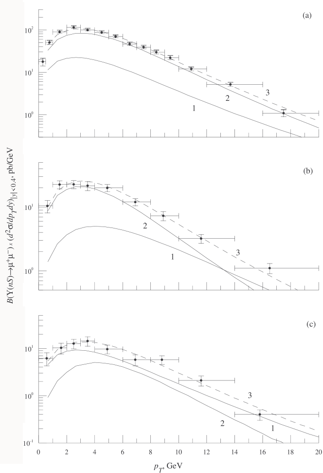
Figure 8: Same as in Fig. 6, but for the KMR KMR un-integrated gluon distribution function.

In Figs. 6, 7, and 8, we compare the CDF data on prompt $\Upsilon(nS)$ hadroproduction in run I CDFBottomI with the theoretical results evaluated with the JB JB , JS JS , and KMR KMR un-integrated gluon distribution functions, respectively, and the NMEs listed in Table 2. In each case, the color-singlet and color-octet contributions are also shown separately. Except for the JB and KMR analyses of $\Upsilon(3S)$ production, the color-octet contributions are always suppressed, especially at low values of $p_{T}$. In the JS analysis, the $\Upsilon(1S)$ and $\Upsilon(2S)$ data are significantly exceeded by the color-singlet contributions for $p_{T}\lesssim 10$ GeV, which explains the poor quality of the fit, with $\chi^{2}/\mbox{d.o.f.}=27$. In the JB analysis, this only happens for $p_{T}\lesssim 2$ GeV, so that the value of $\chi^{2}/\mbox{d.o.f.}$ is lowered by one order of magnitude, being $\chi^{2}/\mbox{d.o.f.}=2.9$. By contrast, the KMR gluon yields an excellent fit, with $\chi^{2}/\mbox{d.o.f.}=0.5$, and will be the only one considered in the following discussion. Comparing the color-singlet and color-octet contributions in Fig. 8, we observe that the latter is dominant in the $\Upsilon(3S)$ case and in the $\Upsilon(2S)$ case for $p_{T}\gtrsim 13$ GeV, while it is of minor importance in the $\Upsilon(1S)$ case in the whole $p_{T}$ range considered. The latter feature is substantiated by the run-II data and is reflected in all their $y$ subintervals, as may be see from Fig. LABEL:fig:CDFBottomII.

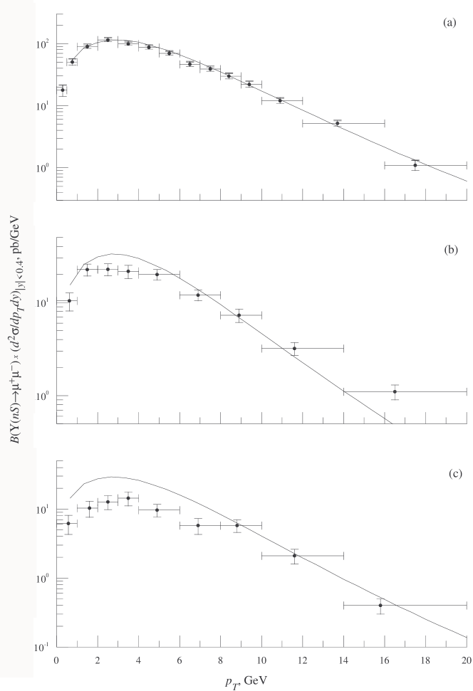
Figure 10: $p_{T}$ distributions of prompt (a) $\Upsilon(1S)$, (b) $\Upsilon(2S)$, and (c) $\Upsilon(3S)$ hadroproduction in $p\overline{p}$ scattering with $\sqrt{S}=1.8$ TeV and $|y|<0.4$ including the respective decay branching fractions $B(\Upsilon(nS)\to\mu^{+}+\mu^{-})$. The color-singlet contribution including the estimated feed-down contributions due to the $\chi_{bJ}(3P)$ meson, evaluated with the KMR KMR un-integrated gluon distribution function, is compared with the CDF data from run I CDFBottomI .

Notice that the contributions to prompt $\Upsilon(nS)$ hadroproduction due to the feed-down from the $\chi_{bJ}(3P)$ mesons have been neglected above, simply because the latter have not yet been observed and their partial decay widths are unknown. In the remainder of this section, we assess the impact of these contributions. For the color-singlet NME, we use the potential model result $\langle{\cal O}^{\chi_{b0}(3P)}[^{3}P_{0}^{(1)}]\rangle=2.7$ GeV⁵ QPM . By analogy to the KMR fit results for $\langle{\cal O}^{\chi_{b0}(1P)}[^{3}S_{1}^{(8)}]\rangle$ and $\langle{\cal O}^{\chi_{b0}(2P)}[^{3}S_{1}^{(8)}]\rangle$ in Table 2, we expect the value of $\langle{\cal O}^{\chi_{b0}(3P)}[^{3}S_{1}^{(8)}]\rangle$ to be negligibly small, compatible with zero. Looking at Table 1, a naive extrapolation from the $\chi_{bJ}(1P)$ and $\chi_{bJ}(2P)$ states suggests that the inclusive branching fractions for the $\chi_{bJ}(3P)$ decays into the $\Upsilon(3S)$, $\Upsilon(2S)$, and $\Upsilon(1S)$ states could be about 12%, 9%, and 7%, respectively. These decays generate further cascade transitions, whose inclusive branching fractions follow from these estimates in combination with the entries of Table 1. Including all these ingredients, we repeat our KMR fit to the CDF data. As illustrated in Fig. 10 for prompt $\Upsilon(nS)$ hadroproduction in run I, the CDF data can be fairly well described in the QMRK approach to the CSM, while the color-octet contributions turn out to be negligibly small. We note in passing that a similar observation, although with lower degree of agreement between data and theory, can be made for the JB gluon, while the JS gluon badly fails for $p_{T}\lesssim 10$ GeV.

V Conclusion

Working at LO in the QMRK approach to NRQCD, we analytically evaluated the squared amplitudes of prompt bottomonium production in two-reggeon collisions. We extracted the relevant color-octet NMEs, $\langle{\cal O}^{\cal H}[^{3}S_{1}^{(8)}]\rangle$, $\langle{\cal O}^{\cal H}[^{1}S_{0}^{(8)}]\rangle$, and $\langle{\cal O}^{\cal H}[^{3}P_{0}^{(8)}]\rangle$ for ${\cal H}=\Upsilon(1S)$, $\Upsilon(2S)$, $\Upsilon(3S)$, $\chi_{b0}(1P)$, and $\chi_{b0}(2P)$, through fits to $p_{T}$ distributions of prompt $\Upsilon(nS)$ hadroproduction measured by the CDF Collaboration at the Tevatron in $p\bar{p}$ collisions with $\sqrt{S}=1.8$ TeV CDFBottomI and 1.96 TeV CDFBottomII using three different un-integrated gluon distribution functions of the proton, namely JB JB , JS JS , and KMR KMR . The fits based on the KMR, JB, and JS gluons turned out to be excellent, fair, and poor, respectively. They yielded small to vanishing values for the color-octet NMEs, especially when the estimated feed-down contributions from the as-yet unobserved $\chi_{bJ}(3P)$ states were included.

The present analysis, together with a recent investigation of charmonium production at high energies KniehlSaleevVasin , suggest that the color-octet NMEs of bottomonium are more strongly suppressed than those of charmonium as expected from the velocity scaling rules of NRQCD. We illustrated that the QMRK approach KTLipatov ; KTAntonov provides a useful laboratory to describe the phenomenology of high-energy processes in the Regge limit of QCD.

LO predictions in both the collinear parton model and the QMRK framework suffer from sizeable theoretical uncertainties, which are largely due to unphysical-scale dependences. Substantial improvement can only be achieved by performing full NLO analyses. While the stage for the NLO NRQCD treatment of $2\to 2$ processes has been set in the collinear parton model kkms , conceptual issues still remain to be elaborated in the QMRK approach. Since, at NLO, incoming partons can gain a finite $k_{T}$ kick through the perturbative emission of partons, one expects that essential features produced by the QMRK approach at LO will thus automatically show up at NLO in the collinear parton model.

VI Acknowledgements

We thank E. Kuraev and M. Ryskin for useful discussions. D.V.V. is grateful to the International Center of Fundamental Physics in Moscow and the Dynastiya Foundation for financial support. This work was supported in part by BMBF Grant No. 05 HT4GUA/4 and by DFG Grant No. KN 365/6–1.

Table 1: Inclusive branching fractions of the feed-down decays of the various bottomonium states.

In$\setminus$Out	$\Upsilon(3S)$	$\chi_{b2}(2P)$	$\chi_{b1}(2P)$	$\chi_{b0}(2P)$	$\Upsilon(2S)$	$\chi_{b2}(1P)$	$\chi_{b1}(1P)$	$\chi_{b0}(1P)$	$\Upsilon(1S)$
$\Upsilon(3S)$	1	0.114	0.113	0.054	0.106	0.00721	0.00742	0.00403	0.102
$\chi_{b2}(2P)$	$\cdots$	1	$\cdots$	$\cdots$	0.162	0.0110	0.0113	0.00616	0.130
$\chi_{b1}(2P)$	$\cdots$	$\cdots$	1	$\cdots$	0.21	0.0143	0.0147	0.00798	0.161
$\chi_{b0}(2P)$	$\cdots$	$\cdots$	$\cdots$	1	0.046	0.00313	0.00322	0.00175	0.0167
$\Upsilon(2S)$	$\cdots$	$\cdots$	$\cdots$	$\cdots$	1	0.068	0.07	0.038	0.320
$\chi_{b2}(1P)$	$\cdots$	$\cdots$	$\cdots$	$\cdots$	$\cdots$	1	$\cdots$	$\cdots$	0.22
$\chi_{b1}(1P)$	$\cdots$	$\cdots$	$\cdots$	$\cdots$	$\cdots$	$\cdots$	1	$\cdots$	0.35
$\chi_{b0}(1P)$	$\cdots$	$\cdots$	$\cdots$	$\cdots$	$\cdots$	$\cdots$	$\cdots$	1	0.06
$\Upsilon(1S)$	$\cdots$	$\cdots$	$\cdots$	$\cdots$	$\cdots$	$\cdots$	$\cdots$	$\cdots$	1

Table 2: NMEs of the $\Upsilon(1S)$, $\Upsilon(2S)$, $\Upsilon(3S)$, $\chi_{b0}(1P)$, and $\chi_{b0}(2P)$ mesons from fits to CDF data from run I CDFBottomI and run II CDFBottomII in the collinear parton model (PM) BFL using the CTEQ5L CTEQ parton distribution functions of the proton and in the QMRK approach using the JB JB , JS JS , and KMR KMR un-integrated gluon distribution functions of the proton. The errors on the fit results are determined by varying in turn each NME up and down about its central value until the value of $\chi^{2}$ is increased by unity keeping all other NMEs fixed at their central values.

NME	PM BFL	Fit JB	Fit JS	Fit KMR
$\langle{\cal O}^{\Upsilon(1S)}[^{3}S_{1}^{(1)}]\rangle/$GeV3	$10.9\pm 1.6$	$10.9\pm 1.6$	$10.9\pm 1.6$	$10.9\pm 1.6$
$\langle{\cal O}^{\Upsilon(1S)}[^{3}S_{1}^{(8)}]\rangle/$GeV3	$\left(2.0\pm 4.1{-0.6\atopwithdelims. .{+0.5}}\right)\times 10^{-2}$	$(5.3\pm 0.5)\times 10^{-3}$	$(0.0\pm 1.8)\times 10^{-4}$	$(0.0\pm 3.1)\times 10^{-3}$
$\langle{\cal O}^{\Upsilon(1S)}[^{1}S_{0}^{(8)}]\rangle/$GeV3	$\cdots$	$(0.0\pm 4.7)\times 10^{-4}$	$(0.0\pm 5.2)\times 10^{-5}$	$(0.0\pm 4.3)\times 10^{-3}$
$\langle{\cal O}^{\Upsilon(1S)}[^{3}P_{0}^{(8)}]\rangle/$GeV5	$\cdots$	$(0.0\pm 1.3)\times 10^{-3}$	$(0.0\pm 1.6)\times 10^{-4}$	$(9.5\pm 2.0)\times 10^{-2}$
$M_{5}^{\Upsilon(1S)}/$GeV3	$\left(1.4\pm 0.7{+1.0\atopwithdelims. .{-0.7}}\right)\times 10^{-1}$	$(0.0\pm 7.6)\times 10^{-4}$	$(0.0\pm 8.7)\times 10^{-5}$	$(2.1\pm 0.9)\times 10^{-2}$
$\langle{\cal O}^{\chi_{b0}(1P)}[^{3}P_{0}^{(1)}]\rangle/$GeV5	$2.4\pm 0.4$	$2.4\pm 0.4$	$2.4\pm 0.4$	$2.4\pm 0.4$
$\langle{\cal O}^{\chi_{b0}(1P)}[^{3}S_{1}^{(8)}]\rangle/$GeV3	$\left(1.5\pm 1.1{+1.3\atopwithdelims. .{-1.0}}\right)\times 10^{-2}$	$(0.0\pm 2.1)\times 10^{-3}$	$(0.0\pm 8.4)\times 10^{-5}$	$(0.0\pm 1.4)\times 10^{-3}$
$\langle{\cal O}^{\Upsilon(2S)}[^{3}S_{1}^{(1)}]\rangle/$GeV3	$4.5\pm 0.7$	$4.5\pm 0.7$	$4.5\pm 0.7$	$4.5\pm 0.7$
$\langle{\cal O}^{\Upsilon(2S)}[^{3}S_{1}^{(8)}]\rangle/$GeV3	$\left(1.6\pm 0.6{+0.7\atopwithdelims. .{-0.5}}\right)\times 10^{-1}$	$(0.0\pm 5.9)\times 10^{-3}$	$(0.0\pm 4.1)\times 10^{-4}$	$(3.3\pm 0.8)\times 10^{-2}$
$\langle{\cal O}^{\Upsilon(2S)}[^{1}S_{0}^{(8)}]\rangle/$GeV3	$\cdots$	$(0.0\pm 9.2)\times 10^{-4}$	$(0.0\pm 8.3)\times 10^{-5}$	$(0.0\pm 3.7)\times 10^{-3}$
$\langle{\cal O}^{\Upsilon(2S)}[^{3}P_{0}^{(8)}]\rangle/$GeV5	$\cdots$	$(0.0\pm 2.6)\times 10^{-3}$	$(0.0\pm 2.8)\times 10^{-4}$	$(0.0\pm 1.6)\times 10^{-2}$
$M_{5}^{\Upsilon(2S)}/$GeV3	$\left(-1.1\pm 1.0{+0.3\atopwithdelims. .{-0.2}}\right)\times 10^{-1}$	$(0.0\pm 1.5)\times 10^{-3}$	$(0.0\pm 1.4)\times 10^{-4}$	$(0.0\pm 7.2)\times 10^{-3}$
$\langle{\cal O}^{\chi_{b0}(2P)}[^{3}P_{0}^{(1)}]\rangle/$GeV5	$2.6\pm 0.5$	$2.6\pm 0.5$	$2.6\pm 0.5$	$2.6\pm 0.5$
$\langle{\cal O}^{\chi_{b0}(2P)}[^{3}S_{1}^{(8)}]\rangle/$GeV3	$\left(0.8\pm 1.1{+1.1\atopwithdelims. .{-0.8}}\right)\times 10^{-2}$	$(1.1\pm 0.4)\times 10^{-2}$	$(0.0\pm 2.8)\times 10^{-4}$	$(0.0\pm 5.7)\times 10^{-3}$
$\langle{\cal O}^{\Upsilon(3S)}[^{3}S_{1}^{(1)}]\rangle/$GeV3	$4.3\pm 0.9$	$4.3\pm 0.9$	$4.3\pm 0.9$	$4.3\pm 0.9$
$\langle{\cal O}^{\Upsilon(3S)}[^{3}S_{1}^{(8)}]\rangle/$GeV3	$\left(3.6\pm 1.9{+1.8\atopwithdelims. .{-1.3}}\right)\times 10^{-2}$	$(1.4\pm 0.3)\times 10^{-2}$	$(5.9\pm 4.2)\times 10^{-3}$	$(1.1\pm 0.4)\times 10^{-2}$
$\langle{\cal O}^{\Upsilon(3S)}[^{1}S_{0}^{(8)}]\rangle/$GeV3	$\cdots$	$(0.0\pm 2.6)\times 10^{-3}$	$(0.0\pm 8.1)\times 10^{-4}$	$(0.0\pm 2.7)\times 10^{-3}$
$\langle{\cal O}^{\Upsilon(3S)}[^{3}P_{0}^{(8)}]\rangle/$GeV5	$\cdots$	$(2.4\pm 0.8)\times 10^{-2}$	$(3.4\pm 4.2)\times 10^{-3}$	$(5.2\pm 1.1)\times 10^{-2}$
$M_{5}^{\Upsilon(3S)}/$GeV3	$\left(5.4\pm 4.3{+3.1\atopwithdelims. .{-2.2}}\right)\times 10^{-2}$	$(5.2\pm 4.4)\times 10^{-3}$	$(7.4\pm 10.2)\times 10^{-4}$	$(1.1\pm 0.5)\times 10^{-2}$
$\langle{\cal O}^{\chi_{b0}(3P)}[^{3}P_{0}^{(1)}]\rangle/$GeV5	$2.7\pm 0.7$	$2.7\pm 0.7$	$2.7\pm 0.7$	$2.7\pm 0.7$
$\chi^{2}/\mathrm{d.o.f.}$	$\cdots$	$2.9$	$27$	$0.5$

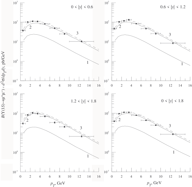
Figure 9: $p_{T}$ distributions of prompt $\Upsilon(1S)$ hadroproduction in $p\overline{p}$ scattering with $\sqrt{S}=1.96$ TeV and (a) $|y|<0.6$, (b) $0.6<|y|<1.2$, (c) $1.2<|y|<1.8$, and (d) $|y|<1.8$ including the decay branching fractions $B(\Upsilon(1S)\to\mu^{+}+\mu^{-})$. The color-octet (curve 1) and color-singlet (curve 2) contributions, evaluated with the KMR KMR un-integrated gluon distribution function, and their sum (curve 3) are compared with the CDF data from run II CDFBottomII .

References

- (1) G. T. Bodwin, E. Braaten, and G. P. Lepage, Phys. Rev. D 51, 1125 (1995); 55, 5853(E) (1997).
- (2) CTEQ Collaboration, R. Brock et al., Rev. Mod. Phys. 67, 157 (1995).
- (3) V. N. Gribov and L. N. Lipatov, Sov. J. Nucl. Phys. 15, 438 (1972) [Yad. Fiz. 15, 781 (1972)]; Yu. L. Dokshitzer, Sov. Phys. JETP 46, 641 (1977) [Zh. Eksp. Teor. Fiz. 73, 1216 (1977)]; G. Altarelli and G. Parisi, Nucl. Phys. B126, 298 (1977).
- (4) E. A. Kuraev, L. N. Lipatov, and V. S. Fadin, Sov. Phys. JETP 44, 443 (1976) [Zh. Eksp. Teor. Fiz. 71, 840 (1976)]; I. I. Balitsky and L. N. Lipatov, Sov. J. Nucl. Phys. 28, 822 (1978) [Yad. Fiz. 28, 1597 (1978)].
- (5) L. V. Gribov, E. M. Levin, and M. G. Ryskin, Phys. Rept. 100, 1 (1983); S. Catani, M. Ciafoloni, and F. Hautmann, Nucl. Phys. B366, 135 (1991).
- (6) J. C. Collins and R. K. Ellis, Nucl. Phys. B360, 3 (1991).
- (7) V. S. Fadin and L. N. Lipatov, Nucl. Phys. B477, 767 (1996).
- (8) E. N. Antonov, L. N. Lipatov, E. A. Kuraev, and I. O. Cherednikov, Nucl. Phys. B721, 111 (2005).
- (9) L. N. Lipatov, Nucl. Phys. B452, 369 (1995).
- (10) V. A. Saleev and D. V. Vasin, Phys. Rev. D 68, 114013 (2003); Phys. Atom. Nucl. 68, 94 (2005) [Yad. Fiz. 68, 95 (2005)].
- (11) B. A. Kniehl, D. V. Vasin, and V. A. Saleev, Phys. Rev. D 73, 074022 (2006).
- (12) Small Collaboration, B. Anderson et al., Eur. Phys. J. C 25, 77 (2002).
- (13) V. S. Fadin, M. I. Kotsky, and L. N. Lipatov, Phys. Lett. B 415, 97 (1997); A. Leonidov and D. Ostrovsky, Eur. Phys. J. C 11, 495 (1999); D. Ostrovsky, Phys. Rev. D 62, 054028 (2000); V. S. Fadin, M. G. Kozlov, and A. V. Reznichenko, Phys. Atom. Nucl. 67, 359 (2004) [Yad. Fiz. 67, 377 (2004)].
- (14) J. Blümlein, Report No. DESY 95–121 (1995).
- (15) H. Jung and G. P. Salam, Eur. Phys. J. C 19, 351 (2001).
- (16) M. A. Kimber, A. D. Martin, and M. G. Ryskin, Phys. Rev. D 63, 114027 (2001).
- (17) V. A. Saleev and D. V. Vasin, Phys. Lett. B 548, 161 (2002).
- (18) M. Ciafaloni, Nucl. Phys. B296, 49 (1988); S. Catani, F. Fiorani, and G. Marchesini, Phys. Lett. B 234, 339 (1990); G. Marchesini, Nucl. Phys. B445, 49 (1995).
- (19) CDF Collaboration, F. Abe et al., Phys. Rev. Lett. 75, 4358 (1995); CDF Collaboration, D. Acosta et al., ibid. 88, 161802 (2002).
- (20) CDF Collaboration, V. M. Abazov et al., Phys. Rev. Lett. 94, 232001 (2005).
- (21) V. G. Kartvelishvili, A. K. Likhoded, and S. R. Slabospitsky, Sov. J. Nucl. Phys. 28, 678 (1978) [Yad. Fiz. 28, 1315 (1978)]; E. L. Berger and D. Jones, Phys. Rev. D 23, 1521 (1981); R. Baier and R. Rückl, Phys. Lett. B 102, 364 (1981).
- (22) N. Brambilla et al., CERN Yellow Report No. CERN-2005-005 and No. FERMILAB-FN-0779, 2005.
- (23) E. Braaten, S. Fleming, and A. K. Leibovich, Phys. Rev. D 63, 094006 (2001).
- (24) J. F. Amundson, O. J. P. Eboli, E. M. Gregores, and F. Halzen, Phys. Lett. B 390, 323 (1997).
- (25) E. L. Berger, J. Qiu, and Y. Wang, Phys. Rev. D 71, 034007 (2005); Int. J. Mod. Phys. A 20, 3753 (2005).
- (26) Particle Data Group, S. Eidelman et al., Phys. Lett. B 592, 1 (2004).
- (27) CTEQ Collaboration, H. L. Lai et al., Eur. Phys. J. C 12, 375 (2000).
- (28) R. Barbieri, R. Gatto, R. Kögerler, and Z. Kunszt, Phys. Lett. B 57, 455 (1975); R. Barbieri, M. Caffo, R. Gatto, and E. Remiddi, Nucl. Phys. B192, 61 (1981).
- (29) W. Lucha, F. F. Schoberl, and D. Gromes, Phys. Rept. 200, 127 (1991); E. J. Eichten and C. Quigg, Phys. Rev. D 52, 1726 (1995).
- (30) M. Klasen, B. A. Kniehl, L. N. Mihaila, and M. Steinhauser, Nucl. Phys. B609, 518 (2001); Phys. Rev. Lett. 89, 032001 (2002); Nucl. Phys. B713, 487 (2005); Phys. Rev. D 71, 014016 (2005).